a robust and accurate binning algorithm for metagenomic sequences with arbitrary species abundance...

[15:08 16/5/2011 Bioinformatics-btr186.tex] Page: 1489 1489–1495

BIOINFORMATICS ORIGINAL PAPER Vol. 27 no. 11 2011, pages 1489–1495doi:10.1093/bioinformatics/btr186

Sequence analysis Advance Access publication April 14, 2011

A robust and accurate binning algorithm for metagenomicsequences with arbitrary species abundance ratioHenry C. M. Leung1,∗, S. M. Yiu1, Bin Yang1, Yu Peng1, Yi Wang1, Zhihua Liu1,Jingchi Chen1, Junjie Qin2, Ruiqiang Li2 and Francis Y. L. Chin1,∗1Department of Computer Science, The University of Hong Kong, Hong Kong SAR and 2Department ofBioinformatics, BGI-Shenzhen, Shenzhen, ChinaAssociate Editor: Alex Bateman

ABSTRACT

Motivation: With the rapid development of next-generationsequencing techniques, metagenomics, also known asenvironmental genomics, has emerged as an exciting researcharea that enables us to analyze the microbial environment inwhich we live. An important step for metagenomic data analysisis the identification and taxonomic characterization of DNAfragments (reads or contigs) resulting from sequencing a sampleof mixed species. This step is referred to as ‘binning’. Binningalgorithms that are based on sequence similarity and sequencecomposition markers rely heavily on the reference genomes ofknown microorganisms or phylogenetic markers. Due to the limitedavailability of reference genomes and the bias and low availabilityof markers, these algorithms may not be applicable in all cases.Unsupervised binning algorithms which can handle fragments fromunknown species provide an alternative approach. However, existingunsupervised binning algorithms only work on datasets either withbalanced species abundance ratios or rather different abundanceratios, but not both.Results: In this article, we present MetaCluster 3.0, an integratedbinning method based on the unsupervised top–down separationand bottom–up merging strategy, which can bin metagenomicfragments of species with very balanced abundance ratios (say 1:1)to very different abundance ratios (e.g. 1:24) with consistently higheraccuracy than existing methods.Availability: MetaCluster 3.0 can be downloaded athttp://i.cs.hku.hk/∼alse/MetaCluster/.Contact: [email protected]; [email protected]

Received and revised on March 22, 2011; accepted on March 29,2011

1 INTRODUCTIONTraditional microbial genomic studies usually focus on one singleindividual bacterial strain due to experimental limitations. In fact,all microorganisms in a habitat have various functional effectson one another and their hosts. For example, the diversity ofmicrobes in humans is shown to be associated with common diseasessuch as inflammatory bowel disease (IBD) (Qin et al., 2010) andgastrointestinal disturbance (Khachatryan et al., 2008). Genomicanalysis on the collective genomes of all microorganisms from

∗To whom correspondence should be addressed.

an environmental sample (known as metagenomics, environmentalgenomics or community genomics) becomes essential. One majordifficulty of metagenomics lies in the fact that most bacteria (up to99%) found in environmental samples are unknown and cannot becultivated and isolated under laboratory conditions (Amann et al.,1990). With high-throughput sequencing technology, one possiblesolution is to directly sequence DNA fragments of multiple speciesobtained from the mixed environmental DNA sample (Venter et al.,2004). Some well-known metagenomics projects, including the AcidMine Drainage Biofilm (AMD) project that analyzes dozens ofspecies (Tyson et al., 2004) and the Human Gut Microbiome (HGM)project that involves thousands of species (Jones et al., 2008), studyfragments obtained from this sequencing approach.

DNA fragments of a metagenomics project are usually frommultiple genomes and most of the genome sequences are unknown.An important step in metagenomic analysis is to group DNAfragments from similar species together (referred to as binning)(Mavromatis et al., 2007) to obtain the microbe distribution of thesample and identify species (including unknown species) within thesample. Depending on different research needs, the binning processcould be performed on different taxonomic levels from Kingdom(the highest level) to Species (the lowest level).

Traditional binning methods can be roughly classified as similaritybased and composition based. Similarity-based methods (Husonet al., 2007) align each DNA fragment to known reference genomes.Based on the alignment results [e.g. BLAST hits or selectedphylogenetic specific marker genes (Altschul et al., 1997)], eachfragment is assigned to the taxonomic class of the similar referencegenomes. Similarity-based methods are usually limited by theavailability of known microorganism genomes given that <1% ofmicroorganisms have been cultured and sequenced.

On the other hand, composition-based methods group DNAfragments in a supervised or semi-supervised manner using genericfeatures such as genome structure or composition. Structuralfeatures, such as composition features of reference genomes ortaxonomic marker regions [e.g. 16S rRNA (Cole et al., 2005), recAand rpoB are commonly accepted fingerprint genes], are extractedand used to construct classifiers (Chan et al., 2008; Chatterji et al.,2008) for determining DNA fragments from different species orconstraints for semi-supervised clustering. These composition-basedmethods usually suffer from the low availability and reliability oftaxonomic markers. For example, studies on the enhanced biologicalphosphorus removing (EBPR) sludge (Garcia Martin et al., 2006),Sargasso Sea (Venter et al., 2004) and the Minnesota soil samples

© The Author 2011. Published by Oxford University Press. All rights reserved. For Permissions, please email: [email protected] 1489

at University of Sydney L

ibrary on August 29, 2014

http://bioinformatics.oxfordjournals.org/

Dow

nloaded from



H.C.M.Leung et al.

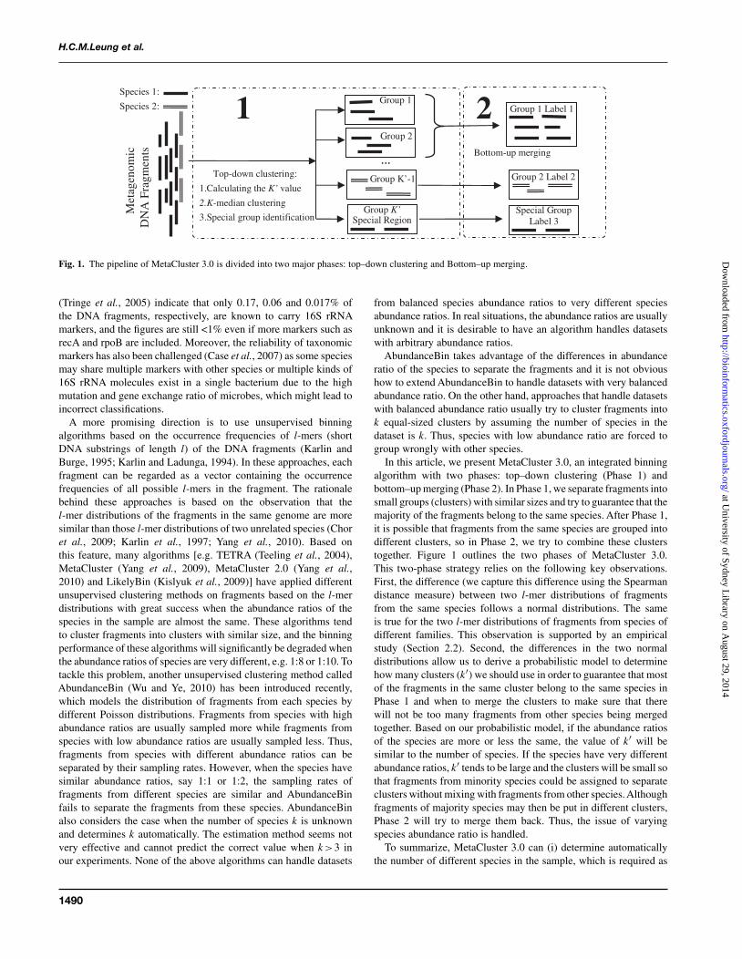
Fig. 1. The pipeline of MetaCluster 3.0 is divided into two major phases: top–down clustering and Bottom–up merging.

(Tringe et al., 2005) indicate that only 0.17, 0.06 and 0.017% ofthe DNA fragments, respectively, are known to carry 16S rRNAmarkers, and the figures are still <1% even if more markers such asrecA and rpoB are included. Moreover, the reliability of taxonomicmarkers has also been challenged (Case et al., 2007) as some speciesmay share multiple markers with other species or multiple kinds of16S rRNA molecules exist in a single bacterium due to the highmutation and gene exchange ratio of microbes, which might lead toincorrect classifications.

A more promising direction is to use unsupervised binningalgorithms based on the occurrence frequencies of l-mers (shortDNA substrings of length l) of the DNA fragments (Karlin andBurge, 1995; Karlin and Ladunga, 1994). In these approaches, eachfragment can be regarded as a vector containing the occurrencefrequencies of all possible l-mers in the fragment. The rationalebehind these approaches is based on the observation that thel-mer distributions of the fragments in the same genome are moresimilar than those l-mer distributions of two unrelated species (Choret al., 2009; Karlin et al., 1997; Yang et al., 2010). Based onthis feature, many algorithms [e.g. TETRA (Teeling et al., 2004),MetaCluster (Yang et al., 2009), MetaCluster 2.0 (Yang et al.,2010) and LikelyBin (Kislyuk et al., 2009)] have applied differentunsupervised clustering methods on fragments based on the l-merdistributions with great success when the abundance ratios of thespecies in the sample are almost the same. These algorithms tendto cluster fragments into clusters with similar size, and the binningperformance of these algorithms will significantly be degraded whenthe abundance ratios of species are very different, e.g. 1:8 or 1:10. Totackle this problem, another unsupervised clustering method calledAbundanceBin (Wu and Ye, 2010) has been introduced recently,which models the distribution of fragments from each species bydifferent Poisson distributions. Fragments from species with highabundance ratios are usually sampled more while fragments fromspecies with low abundance ratios are usually sampled less. Thus,fragments from species with different abundance ratios can beseparated by their sampling rates. However, when the species havesimilar abundance ratios, say 1:1 or 1:2, the sampling rates offragments from different species are similar and AbundanceBinfails to separate the fragments from these species. AbundanceBinalso considers the case when the number of species k is unknownand determines k automatically. The estimation method seems notvery effective and cannot predict the correct value when k >3 inour experiments. None of the above algorithms can handle datasets

from balanced species abundance ratios to very different speciesabundance ratios. In real situations, the abundance ratios are usuallyunknown and it is desirable to have an algorithm handles datasetswith arbitrary abundance ratios.

AbundanceBin takes advantage of the differences in abundanceratio of the species to separate the fragments and it is not obvioushow to extend AbundanceBin to handle datasets with very balancedabundance ratio. On the other hand, approaches that handle datasetswith balanced abundance ratio usually try to cluster fragments intok equal-sized clusters by assuming the number of species in thedataset is k. Thus, species with low abundance ratio are forced togroup wrongly with other species.

In this article, we present MetaCluster 3.0, an integrated binningalgorithm with two phases: top–down clustering (Phase 1) andbottom–up merging (Phase 2). In Phase 1, we separate fragments intosmall groups (clusters) with similar sizes and try to guarantee that themajority of the fragments belong to the same species. After Phase 1,it is possible that fragments from the same species are grouped intodifferent clusters, so in Phase 2, we try to combine these clusterstogether. Figure 1 outlines the two phases of MetaCluster 3.0.This two-phase strategy relies on the following key observations.First, the difference (we capture this difference using the Spearmandistance measure) between two l-mer distributions of fragmentsfrom the same species follows a normal distributions. The sameis true for the two l-mer distributions of fragments from species ofdifferent families. This observation is supported by an empiricalstudy (Section 2.2). Second, the differences in the two normaldistributions allow us to derive a probabilistic model to determinehow many clusters (k′) we should use in order to guarantee that mostof the fragments in the same cluster belong to the same species inPhase 1 and when to merge the clusters to make sure that therewill not be too many fragments from other species being mergedtogether. Based on our probabilistic model, if the abundance ratiosof the species are more or less the same, the value of k′ will besimilar to the number of species. If the species have very differentabundance ratios, k′ tends to be large and the clusters will be small sothat fragments from minority species could be assigned to separateclusters without mixing with fragments from other species.Althoughfragments of majority species may then be put in different clusters,Phase 2 will try to merge them back. Thus, the issue of varyingspecies abundance ratio is handled.

To summarize, MetaCluster 3.0 can (i) determine automaticallythe number of different species in the sample, which is required as

1490




Dow

nloaded from



Binning algorithm for metagenomic sequences

an input parameter for most unsupervised algorithms (Kislyuk et al.,2009; Teeling et al., 2004; Yang et al., 2009; 2010) and (ii) classifyaccurately the metagenomic fragments with balanced speciesabundance ratios, which cannot be handled by AbundanceBin (Wuand Ye, 2010), to very different species abundance ratio, whichcannot be handled by other unsupervised algorithms (Kislyuk et al.,2009; Teeling et al., 2004; Yang et al., 2009; 2010) and combinationsof these situations, say 1:3:3:9, which cannot be handled by anyunsupervised algorithms.

2 METHODSIn this section, we first define the l-mer feature vector of a fragmentthat captures the l-mer frequency distribution of the fragment. Then, wedescribe the Spearman Footrule distance (Diaconis and Graham, 1977) torepresent the difference (distance) between two l-mer feature vectors or theircorresponding fragments. We have also tried different similarity measuressuch as Kendall’s Tau (Kendall, 1938) and those mentioned in Wu and Ye(2010); Yang et al. (2009). Spearman Footrule distance seems to be betterin terms of performance in our clustering and computational complexity.We remark that there may also be other measures which are appropriate tosolve the problem. Next, we will show the result of an empirical study whichconfirms our key observations. Lastly, we describe the details of top–downclustering (Phase 1) and bottom–up merging (Phase 2) together with ourprobabilistic model which is used to determine the number of clusters to beused in Phase 1 and when to merge two clusters in Phase 2.

2.1 l-mer frequency and distance definitionThe DNA composition features of each DNA fragment are represented bythe l-mer frequencies of the DNA fragment. As there are four different DNAnucleotides, there are at most 4l kinds of l-mers in a DNA sequence. If asliding window of width l is slid along each DNA fragment of length n andthe frequency of every l-mer, say fw, w∈{A,C,G,T}l , is recorded, the totalnumber of l-mers in a DNA fragment would be

∑fw =n−l+1. For example,

a DNA fragment of length 500 nt has 497 4-mers. The DNA feature vectoris defined as [f1, f2, ..., fN(l)], where N(l) is the number of different l-mers.As each DNA fragment can be obtained from either strand of the DNAgenome, the frequency of one l-mer and its reverse complement l-mer canbe combined together and this process will reduce the size of vector by half,i.e. N(l)=4l/2, if l is odd; N(l)= (4l +4l/2)/2, if l is even.

As mentioned in Chor et al. (2009) and Zhou et al. (2008), setting l=4is the best (among l=2−7) when barcoding a genome with DNA fragmentsize from 1000 nt to 10 000 nt. Each DNA fragment will be represented by afeature vector with 136 components and the input metagenomic sequencingdataset can be transformed to an n×136 matrix with n rows representingn DNA fragments. Our binning method is based on the observation (Choret al., 2009; Teeling et al., 2004) that the l-mer distributions of those DNAsubstrings (fragments) from the same genome are similar. The similarity of4-mer distribution is not limited to the coding region but the whole genomesequence (Chor et al., 2009; Zhou et al., 2008). We compute the differenceof two l-mer distributions from two fragments by measuring the SpearmanFootrule distance between their corresponding l-mer feature vectors.

Spearman Footrule distance (henceforth referred as Spearman distance)is defined as follows. Consider two DNA fragments A and B with thefollowing 4-mer feature vectors A: (a1,a2, ... ,aN(l)) and B: (b1,b2, ... ,bN(l)).The Spearman distance is based on an intuitive definition for comparing twoordered lists. Let rA(ai) be the rank of ai in the sorted list of ai’s and rA(bi) bethe rank of bi in the sorted list of bi’s. Then the Spearman distance is definedas dists(A,B)=∑|rA(ai)−rB(bi)|. The smaller the value of the metric, themore similar the vectors are. For vectors with size k, the distance value canrange between 0 and k(k+1). Compared with other distance metrics that relyon the exact value of each entry in the feature vectors, Spearman distance,which relies on the rank of the entries, is less sensitive to those entries with

Fig. 2. Probability density functions of the Spearman distance betweentwo fragments from the same species (intradistance) and between twofragments from the same order but different families (interdistance).Approx intradistance and approx interdistance is the normal distributionapproximation of the two distances.

unexpectedly large values. Moreover, the Spearman distance gives a moreglobal view of the distance of two feature vectors with respected to all theentries.

2.2 Spearman distance distributionTo confirm our observation that both the Spearman distance distributionsof the differences between two l-mer distributions of fragments (pairwisefragment distances) from the same species and those from species of differentfamilies can be approximated by a normal distribution, we conduct anempirical study for 1000 genomes. For each genome, we randomly select1 million pairs of fragments of 1000 nt long, and compute the Spearmandistances of all pairs. This distance distribution is referred as intradistancedistribution (Fig. 2). For fragments from different families, we select 10 000pairs of genomes in which the two genomes of each pair belong to differentfamilies but the same order. For each pair of genomes, we select onefragment of length 1000 nt from each genome and compute the Spearmandistance of these two fragments. We repeat this randomly for 1 millionpairs of fragments. This distance distribution is referred as the interdistancedistribution (Fig. 2). From our empirical study, we can see that thesetwo distributions can be approximated by normal distributions and thereis a significant difference between these two distributions. Although thedistribution can be modeled by a mixed Gaussian distribution because ofdifferences in inter and intra distances among different genomes, as weassume that there is no information of the species in the mixture, we usednormal distribution for approximation only. In the following, we describethe details of the two phases (top–down clustering and bottom–up merging)and how we make use of the difference in the intradistance and interdistancedistributions to guarantee the accuracy of these two phases in MetaCluster3.0.

2.3 Top–down clusteringIn this step, we apply the k-median algorithm1(Jain and Dubes, 1981) tocluster the fragments into k′ clusters of similar sizes. k-median algorithmrepeatedly assigns feature vector to the closest cluster and select a featurevector in each cluster as the center with the following objective function

MinE =k′∑

i=1

∑A∈Ci

dists(A,ci)

where feature vector ci is the center of cluster Ci and dists(A, ci) is thespearman distance between feature vectors A and ci.

1We use k-median clustering algorithm as it is easy to compute. Furtherinvestigation on the effectiveness of different clustering algorithms shouldbe conducted.

1491




Dow

nloaded from



H.C.M.Leung et al.

In MetaCluster 3.0, the value of k′ is determined automatically based ona probabilistic model by restricting the expected number of false positivefragments (from other species) in a cluster to be limited by some predefinedthreshold t× size of the cluster, t ∈ (0,1]. The details of how to determinek′ are given below. Since the k-median algorithm is a greedy algorithm, itis repeated several dozen times with different initial clustering centers. Theone that gives the minimum objective function value will be selected.

Now, we show how to determine k′. By dividing n fragments into k′clusters, the average cluster size is n/k′. In each cluster, there are two sets offragments, fragments from the same species as the center and fragments fromspecies different from the center. The distance between each fragment andthe center from the same species can be approximated by N(µintra,σ

2intra)

while the distance between each fragment and the center from differentspecies can be approximated by N(µinter,σ

2inter) (Fig. 2). Given a cluster

Ci with the total distance between the center ci and each feature vectorin the cluster

∑A∈Ci dists(A,ci) equals a particular value di. If s out of

n/k′ fragments (including the center) in the cluster are sampled from thesame species with average distance (intraspecies distance) between the centerand the rest s−1 fragments being x, the probability that there are n/k′ −sfalse positives equals the probability that the average distance (interspeciesdistance) between the center and the n/k′ −s fragments from different specieswill be (di −(s−1)x)/(n/k′ −s), which follows the Gaussian distributionN(µinter,σ

2inter/(n/k′ −s)). By considering all possible values of s and x, the

expected number of false positives in a cluster can be calculated as follows

n/k′∑s=2

s∫ ∞

0fµintra,σ

2intra

/(s−1)(x)

[∫ (di−(s−1)x)/(n/k′−s)

0fµinter,σ

2inter

/(n/k′−s)(y)dy

]dx

where fµ,σ2(x)=e−(x−µ)2/(2σ2)/√

2πσ2 is the probability density function ofa normal distribution with mean µ and variance σ2.

Since the expected number of false positives decreases with the value ofk′, MetaCluster 3.0 increases the value of k′ until the expected number offalse positives in a cluster ≤ tn/k′. In the experiments, we set t =5% suchthat the expected accuracy is over 95% for the first phase. Based on the abovecalculation, we expect that k′ can be much larger than the number of speciesif the species have very different abundance ratios such that fragments fromspecies with high abundance ratios will be divided into more clusters whilefragments from species with low abundance ratios will be grouped into asingle cluster or fewer clusters.

As for the same genome, the l-mer distribution of some special genomeregion (such as insertion and exogenous transferred regions) can be verydifferent from general genome regions. These data points could be consideredoutliers and should be removed. In MetaCluster 3.0, those data points withcenter distance larger than µ+2σ should be removed as outliers, where µ

and σ are the average distance and standard deviation between a data point inthe cluster and the center, respectively. In some cases, the number of outlierDNA fragments from the majority species could be very large and might havespecial biological meaning. So these fragments will be grouped together assome special clusters which will be excluded from the merging phase, butreported specifically for the attention of biologists.

2.4 Bottom–up merging of the clustersAfter dividing the DNA fragments into k′ clusters, a bottom–up mergingphase is introduced to merge the clusters from the same species into onecluster based on the intercluster similarity, i.e. intercluster distance. Theintercluster distance of cluster C1 and cluster C2 is taken to be the averageof all distances between pairs of DNA fragments A in C1 and B in C2.

dist(C1,C2)=∑

A∈C1

∑B∈C2

dists(A,B)

|C1|·|C2|When the number of species k in the sample is known, MetaCluster 3.0merges the pair of clusters with the minimum intercluster distance greedilyuntil there are k large clusters. In practical situations, the number of speciesk is usually unknown and MetaCluster 3.0 should determine when to stop

merging so that clusters that contain fragments from different species willnot be merged into a cluster. Based on the observation that the Spearmandistance between two fragments from the same species is usually smallerthan the Spearman distance between two fragments from different species,MetaCluster 3.0 merges two clusters C1 and C2 with average intraclusterdistance d1 and d2, respectively, if and only if the intercluster distancedist(C1, C2) is similar to d1 and d2, i.e. α dist(C1, C2)≤average(d1, d2)for some threshold α∈ (0,1]. The value of threshold α can be determinedby minimizing the expected false negative and false positive fragments.Assume all fragments in C1(C2) are sampled from the same species, theintracluster distance can be modeled by the intraspecies distance distribution.The probability that MetaCluster 3.0 does not merge two clusters incorrectly(false negative) can be calculated as follow:

P(false negative)=∫ ∞

0fµintra,σ2

intra(x)

∫ ∞

x/αfµintra,σ2

intra(y)dydx (1)

Similarly, the probability that MetaCluster 3.0 merges two clustersincorrectly (false positive) can be calculated.

P(false positive)=∫ ∞

0fµintra,σ

2intra

(x)∫ x/α

0fµinter,σ

2inter

(y)dydx (2)

For the parameters estimated from bacteria genome, setting the thresholdα=0.79 can minimize the expected false negative and false positive (1) + (2)fragments. This threshold is similar to the optimal threshold α=0.83 foundin the simulated data. Unlike all other unsupervised approaches which donot provide any taxonomic annotation for the clusters, MetaCluster 3.0 canlabel (annotate) the clusters with taxonomic information by calculating theaverage Spearman distance between each cluster and the 4mer feature vectorsof the known genome. Although many genomes are still unknown, it willprovide an approximated annotation at high taxonomic ranks such as Familyor Order, which helps the biologists to determine followup experiments forfurther investigation.

3 RESULTSIn this section, we analyze the performance of the binning algorithm,MetaCluster 3.0, based on the simulated metagenomic datasets. Wecompare the performance of MetaCluster 3.0 with AbundanceBin(Wu and Ye, 2010) and our previous version MetaCluster 2.0 (Yanget al., 2009). We have not compared other unsupervised binningalgorithms because MetaCluster 2.0 outperforms these algorithmsin similar experimental setting (Yang et al., 2009). We use thedefault parameters for AbundanceBin and MetaCluster 2.0. Wehave conducted three sets of experiments. (i) We fix the numberof species to be 2 and vary the abundance ratio from the balancedsituation 1:1 to the unbalanced situation of 1:24. We assume thatthe number of species in the dataset is known. The performance ofMetaCluster 3.0 is consistently more accurate for all datasets withdifferent abundance ratios. (ii) We also compare the performance ofMetaCluster 3.0 with AbundanceBin based on datasets with morespecies with different abundance ratios. In this set of experiments,we also assume that the number of species is known. The resultsshow that MetaCluster 3.0 outperformsAbundanceBin. In particular,the accuracy of MetaCluster 3.0 is three times better than thatof AbundanceBin when the species abundance ratio is balanced.(iii) Lastly, we demonstrate that MetaCluster 3.0 works better thanAbundanceBin if the number of species in the dataset is unknown.In all the experiments, we use the parameters t =5% and α=0.8.We have varied the parameters and the results are similar.

1492




Dow

nloaded from




A B

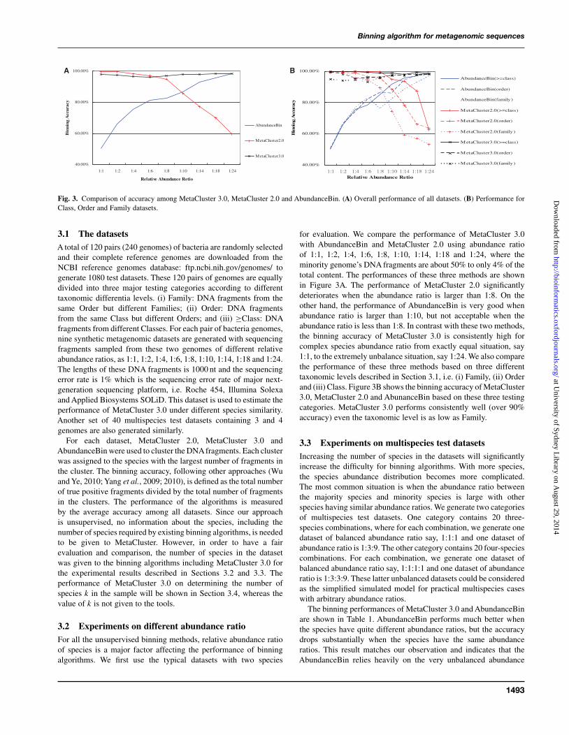
Fig. 3. Comparison of accuracy among MetaCluster 3.0, MetaCluster 2.0 and AbundanceBin. (A) Overall performance of all datasets. (B) Performance forClass, Order and Family datasets.

3.1 The datasetsA total of 120 pairs (240 genomes) of bacteria are randomly selectedand their complete reference genomes are downloaded from theNCBI reference genomes database: ftp.ncbi.nih.gov/genomes/ togenerate 1080 test datasets. These 120 pairs of genomes are equallydivided into three major testing categories according to differenttaxonomic differentia levels. (i) Family: DNA fragments from thesame Order but different Families; (ii) Order: DNA fragmentsfrom the same Class but different Orders; and (iii) ≥Class: DNAfragments from different Classes. For each pair of bacteria genomes,nine synthetic metagenomic datasets are generated with sequencingfragments sampled from these two genomes of different relativeabundance ratios, as 1:1, 1:2, 1:4, 1:6, 1:8, 1:10, 1:14, 1:18 and 1:24.The lengths of these DNA fragments is 1000 nt and the sequencingerror rate is 1% which is the sequencing error rate of major next-generation sequencing platform, i.e. Roche 454, Illumina Solexaand Applied Biosystems SOLiD. This dataset is used to estimate theperformance of MetaCluster 3.0 under different species similarity.Another set of 40 multispecies test datasets containing 3 and 4genomes are also generated similarly.

For each dataset, MetaCluster 2.0, MetaCluster 3.0 andAbundanceBin were used to cluster the DNAfragments. Each clusterwas assigned to the species with the largest number of fragments inthe cluster. The binning accuracy, following other approaches (Wuand Ye, 2010; Yang et al., 2009; 2010), is defined as the total numberof true positive fragments divided by the total number of fragmentsin the clusters. The performance of the algorithms is measuredby the average accuracy among all datasets. Since our approachis unsupervised, no information about the species, including thenumber of species required by existing binning algorithms, is neededto be given to MetaCluster. However, in order to have a fairevaluation and comparison, the number of species in the datasetwas given to the binning algorithms including MetaCluster 3.0 forthe experimental results described in Sections 3.2 and 3.3. Theperformance of MetaCluster 3.0 on determining the number ofspecies k in the sample will be shown in Section 3.4, whereas thevalue of k is not given to the tools.

3.2 Experiments on different abundance ratioFor all the unsupervised binning methods, relative abundance ratioof species is a major factor affecting the performance of binningalgorithms. We first use the typical datasets with two species

for evaluation. We compare the performance of MetaCluster 3.0with AbundanceBin and MetaCluster 2.0 using abundance ratioof 1:1, 1:2, 1:4, 1:6, 1:8, 1:10, 1:14, 1:18 and 1:24, where theminority genome’s DNA fragments are about 50% to only 4% of thetotal content. The performances of these three methods are shownin Figure 3A. The performance of MetaCluster 2.0 significantlydeteriorates when the abundance ratio is larger than 1:8. On theother hand, the performance of AbundanceBin is very good whenabundance ratio is larger than 1:10, but not acceptable when theabundance ratio is less than 1:8. In contrast with these two methods,the binning accuracy of MetaCluster 3.0 is consistently high forcomplex species abundance ratio from exactly equal situation, say1:1, to the extremely unbalance situation, say 1:24. We also comparethe performance of these three methods based on three differenttaxonomic levels described in Section 3.1, i.e. (i) Family, (ii) Orderand (iii) Class. Figure 3B shows the binning accuracy of MetaCluster3.0, MetaCluster 2.0 and AbunanceBin based on these three testingcategories. MetaCluster 3.0 performs consistently well (over 90%accuracy) even the taxonomic level is as low as Family.

3.3 Experiments on multispecies test datasetsIncreasing the number of species in the datasets will significantlyincrease the difficulty for binning algorithms. With more species,the species abundance distribution becomes more complicated.The most common situation is when the abundance ratio betweenthe majority species and minority species is large with otherspecies having similar abundance ratios. We generate two categoriesof multispecies test datasets. One category contains 20 three-species combinations, where for each combination, we generate onedataset of balanced abundance ratio say, 1:1:1 and one dataset ofabundance ratio is 1:3:9. The other category contains 20 four-speciescombinations. For each combination, we generate one dataset ofbalanced abundance ratio say, 1:1:1:1 and one dataset of abundanceratio is 1:3:3:9. These latter unbalanced datasets could be consideredas the simplified simulated model for practical multispecies caseswith arbitrary abundance ratios.

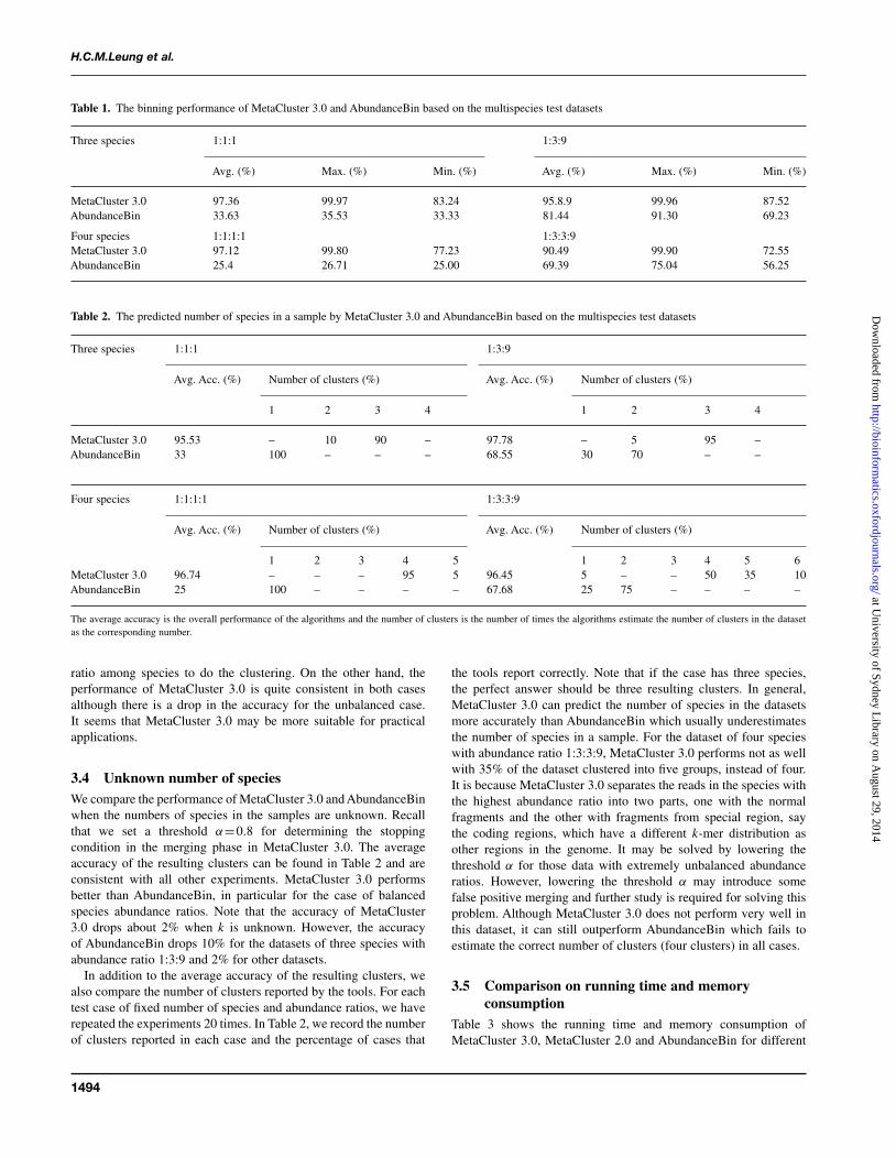
The binning performances of MetaCluster 3.0 and AbundanceBinare shown in Table 1. AbundanceBin performs much better whenthe species have quite different abundance ratios, but the accuracydrops substantially when the species have the same abundanceratios. This result matches our observation and indicates that theAbundanceBin relies heavily on the very unbalanced abundance

1493




Dow

nloaded from



H.C.M.Leung et al.

Table 1. The binning performance of MetaCluster 3.0 and AbundanceBin based on the multispecies test datasets

Three species 1:1:1 1:3:9

Avg. (%) Max. (%) Min. (%) Avg. (%) Max. (%) Min. (%)

MetaCluster 3.0 97.36 99.97 83.24 95.8.9 99.96 87.52AbundanceBin 33.63 35.53 33.33 81.44 91.30 69.23

Four species 1:1:1:1 1:3:3:9MetaCluster 3.0 97.12 99.80 77.23 90.49 99.90 72.55AbundanceBin 25.4 26.71 25.00 69.39 75.04 56.25

Table 2. The predicted number of species in a sample by MetaCluster 3.0 and AbundanceBin based on the multispecies test datasets

Three species 1:1:1 1:3:9

Avg. Acc. (%) Number of clusters (%) Avg. Acc. (%) Number of clusters (%)

1 2 3 4 1 2 3 4

MetaCluster 3.0 95.53 – 10 90 – 97.78 – 5 95 –AbundanceBin 33 100 – – – 68.55 30 70 – –

Four species 1:1:1:1 1:3:3:9

Avg. Acc. (%) Number of clusters (%) Avg. Acc. (%) Number of clusters (%)

1 2 3 4 5 1 2 3 4 5 6MetaCluster 3.0 96.74 – – – 95 5 96.45 5 – – 50 35 10AbundanceBin 25 100 – – – – 67.68 25 75 – – – –

The average accuracy is the overall performance of the algorithms and the number of clusters is the number of times the algorithms estimate the number of clusters in the datasetas the corresponding number.

ratio among species to do the clustering. On the other hand, theperformance of MetaCluster 3.0 is quite consistent in both casesalthough there is a drop in the accuracy for the unbalanced case.It seems that MetaCluster 3.0 may be more suitable for practicalapplications.

3.4 Unknown number of speciesWe compare the performance of MetaCluster 3.0 and AbundanceBinwhen the numbers of species in the samples are unknown. Recallthat we set a threshold α=0.8 for determining the stoppingcondition in the merging phase in MetaCluster 3.0. The averageaccuracy of the resulting clusters can be found in Table 2 and areconsistent with all other experiments. MetaCluster 3.0 performsbetter than AbundanceBin, in particular for the case of balancedspecies abundance ratios. Note that the accuracy of MetaCluster3.0 drops about 2% when k is unknown. However, the accuracyof AbundanceBin drops 10% for the datasets of three species withabundance ratio 1:3:9 and 2% for other datasets.

In addition to the average accuracy of the resulting clusters, wealso compare the number of clusters reported by the tools. For eachtest case of fixed number of species and abundance ratios, we haverepeated the experiments 20 times. In Table 2, we record the numberof clusters reported in each case and the percentage of cases that

the tools report correctly. Note that if the case has three species,the perfect answer should be three resulting clusters. In general,MetaCluster 3.0 can predict the number of species in the datasetsmore accurately than AbundanceBin which usually underestimatesthe number of species in a sample. For the dataset of four specieswith abundance ratio 1:3:3:9, MetaCluster 3.0 performs not as wellwith 35% of the dataset clustered into five groups, instead of four.It is because MetaCluster 3.0 separates the reads in the species withthe highest abundance ratio into two parts, one with the normalfragments and the other with fragments from special region, saythe coding regions, which have a different k-mer distribution asother regions in the genome. It may be solved by lowering thethreshold α for those data with extremely unbalanced abundanceratios. However, lowering the threshold α may introduce somefalse positive merging and further study is required for solving thisproblem. Although MetaCluster 3.0 does not perform very well inthis dataset, it can still outperform AbundanceBin which fails toestimate the correct number of clusters (four clusters) in all cases.

3.5 Comparison on running time and memoryconsumption

Table 3 shows the running time and memory consumption ofMetaCluster 3.0, MetaCluster 2.0 and AbundanceBin for different

1494




Dow

nloaded from




Table 3. The running time and memory consumption of MetaCluster 3.0, MetaCluster 2.0 and AbundanceBin for different dataset size

Running time Memory comsumption

10 000 fragments 50 000 fragments 100 000 fragments 10 000 fragments 50 000 fragments 100 000 fragments

MetaCluster 3.0 15 s 5 min 17 min 173 M 354 M 581 MMetaCluster 2.0 14 s 5 min 18 s 20 min 175 M 356 M 583 MAbundanceBin 2 min 21 s 18 min 37 min 683 M 1.40 G 1.98 G

dataset sizes. The running times of the three algorithms increasewith the input sizes. The running time of MetaCluster 3.0 andMetaCluster 2.0 are similar and much shorter than the running timeof AbundanceBin, as AbundanceBin is required to construct a modelfor the distribution of reads and to repeat clustering the reads toestimate the number of clusters. The memory consumption of thethree algorithms also increases with the input size but MetaCluster3.0 consumes the least amount of memory.

4 CONCLUSIONSIn this article, we propose a two-phase unsupervised binningalgorithm to bin metagenomic fragments with mixed speciesabundance ratios. Based on the differences in the distribution ofa distance measure between fragments of the same species andfragments from different species, our approach can guarantee thequality of our resulting clusters. The performance of our approach,MetaCluster 3.0, is shown to be better than all existing unsupervisedalgorithms. However, binning metagenomic fragments remains achallenging problem.All existing algorithms (including MetaCluster3.0) can only handle datasets with not too many species and theaccuracy decrease sharply when the number of species is over 10. Inthe practical situations, a sample may contain genomes of thousandsof kinds of species for which all existing binning tools fail.

Another limitation of MetaCluster 3.0, is it only works onfragments with length at least 500 nt. As the current high-throughputsequencing technology produces reads with lengths from 50 nt to150 nt only, MetaCluster 3.0 relies on assembly tools for producinghigh-quality contigs with longer lengths. However, some binningalgorithms, e.g. AbundanceBin, can work directly on short reads.Further research is required to come up with an effective tool forbinning short reads directly with mixed species abundance ratio orassembling reads in metagenomic data accurately.

Funding: GRF grant (HKU 719709E, HKU 711611 and HKUSPACE Research Fund) in part.

Conflict of Interest: none declared.

REFERENCESAltschul,S.F. et al. (1997) Gapped BLAST and PSI-BLAST: a new generation of protein

database search programs. Nucleic Acids Res., 25, 3389–3402.Amann,R.I. et al. (1990) Combination of 16S rRNA-targeted oligonucleotide probes

with flow cytometry for analyzing mixed microbial populations. Appl. Environ.Microbiol., 56, 1919–1925.

Case,R.J. et al. (2007) Use of 16S rRNA and rpoB genes as molecular markers formicrobial ecology studies. Appl. Environ. Microbiol., 73, 278–288.

Chan,C.K. et al. (2008) Binning sequences using very sparse labels within ametagenome. BMC Bioinformatics, 9, 215.

Chatterji,S. et al. (2008) A DNA composition-based algorithm for binningenvironmental shotgun reads. Res. Comp. Mole. Biol., 17–28.

Chor,B. et al. (2009) Genomic DNA k-mer spectra: models and modalities. GenomeBiol., 10, R108.

Cole,J.R. et al. (2005) The Ribosomal Database Project (RDP-II): sequences and toolsfor high-throughput rRNA analysis. Nucleic Acids Res., 33, D294–D296.

Diaconis,P. and Graham, R.L. (1977) Spearman’s Footrule as a measure of disarray.J. R. Stat. Soc. Ser. B, 39, 262–268.

Garcia Martin, H. et al. (2006) Metagenomic analysis of two enhanced biologicalphosphorus removal (EBPR) sludge communities. Nat. Biotechnol., 24, 1263–1269.

Huson,D.H. et al. (2007) MEGAN analysis of metagenomic data. Genome Res., 17,377–386.

Jain,A.K. and Dubes,R.C. (1981) Algorithms for Clustering Data. Prentice-Hall, UpperSaddle River, NJ, USA.

Jones,B.V. et al. (2008) Functional and comparative metagenomic analysis of bile salthydrolase activity in the human gut microbiome. Proc. Natl Acad. Sci. USA, 105,13580–13585.

Karlin,S. and Burge,C. (1995) Dinucleotide relative abundance extremes: a genomicsignature. Trends Genet., 11, 283–290.

Karlin,S. and Ladunga,I. (1994) Comparisons of eukaryotic genomic sequences.Proc. Natl Acad. Sci. USA, 91, 12832–12836.

Karlin,S., et al. (1997) Compositional biases of bacterial genomes and evolutionaryimplications. J. Bacteriol., 179, 3899–3913.

Kendall,M.G. (1938) A new measure of rank correlation. Biometrika, 30, 81–93.Khachatryan,Z.A. et al. (2008) Predominant role of host genetics in controlling the

composition of gut microbiota. PLoS One, 3, e3064.Kislyuk, A. et al. (2009) Unsupervised statistical clustering of environmental shotgun

sequences. BMC Bioinformatics, 10, 316.Mavromatis,K. et al. (2007) Use of simulated data sets to evaluate the fidelity of

metagenomic processing methods. Nat. Methods, 4, 495–500.Qin,J. et al. (2010) A human gut microbial gene catalogue established by metagenomic

sequencing. Nature, 464, 59–65.Teeling,H. et al. (2004) TETRA: a web-service and a stand-alone program for the

analysis and comparison of tetranucleotide usage patterns in DNA sequences. BMCBioinformatics, 5, 163.

Tringe,S.G. et al. (2005) Comparative metagenomics of microbial communities.Science, 308, 554–557.

Tyson,G.W. et al. (2004) Community structure and metabolism through reconstructionof microbial genomes from the environment. Nature, 428, 37–43.

Venter,J.C. et al. (2004) Environmental genome shotgun sequencing of the SargassoSea. Science, 304, 66–74.

Wu,Y.W. and Ye,Y. (2010)Anovel abundance-based algorithm for binning metagenomicsequences using l-tuples. Res. Comp. Mole. Biol., 535–549.

Yang,B. et al. (2009) Unsupervised binning of environmental genomic fragments basedon an error robust selection of l-mers. In Data and Text Mining in BiomedicalInformatics ’09, pp. 3–10.

Yang,B. et al. (2010) MetaCluster: unsupervised binning of environmental genomicfragments and taxonomic annotation. In ACM Conference on Bioinformatics,Computational Biology and Biomedicine (ACM-BCB), pp. 170–179.

Zhou,F. et al. (2008) Barcodes for genomes and applications. BMC Bioinformatics,9, 546.

1495




Dow

nloaded from


a robust and accurate binning algorithm for metagenomic sequences with arbitrary species abundance...

Documents