a review of quantum cellular automata

A review of Quantum Cellular AutomataTerry Farrelly∗1,2

1Institut fur Theoretische Physik, Leibniz Universitat Hannover, 30167 Hannover, Germany2ARC Centre for Engineered Quantum Systems, School of Mathematics and Physics, University of Queensland, Brisbane,

QLD 4072, Australia

Discretizing spacetime is often a natural step towards modelling physical systems.For quantum systems, if we also demand a strict bound on the speed of informationpropagation, we get quantum cellular automata (QCAs). These originally arose as analternative paradigm for quantum computation, though more recently they have foundapplication in understanding topological phases of matter and have been proposed asmodels of periodically driven (Floquet) quantum systems, where QCA methods wereused to classify their phases. QCAs have also been used as a natural discretization ofquantum field theory, and some interesting examples of QCAs have been introducedthat become interacting quantum field theories in the continuum limit. This reviewdiscusses all of these applications, as well as some other interesting results on thestructure of quantum cellular automata, including the tensor-network unitary approach,the index theory and higher dimensional classifications of QCAs.

∗ [email protected]

Accepted in Quantum 2020-10-06, click title to verify. Published under CC-BY 4.0. 1

arX

iv:1

904.

1331

8v2

[qu

ant-

ph]

25

Nov

202

0

https://quantum-journal.org/?s=\textbf%20A%20review%20of%20Quantum%20Cellular%20Automata&reason=title-click

Contents

1 Introduction 4

1.1 Two examples of QCAs . . . . . . . . . . . . . . . . . . . . . . . . . . . . . . . . . 61.2 Things that are not QCAs . . . . . . . . . . . . . . . . . . . . . . . . . . . . . . . . 7

2 Definition 8

2.1 Systems . . . . . . . . . . . . . . . . . . . . . . . . . . . . . . . . . . . . . . . . . . 82.2 Dynamics . . . . . . . . . . . . . . . . . . . . . . . . . . . . . . . . . . . . . . . . . 92.3 Global and local transition rules . . . . . . . . . . . . . . . . . . . . . . . . . . . . 112.4 Finite, unbounded configurations . . . . . . . . . . . . . . . . . . . . . . . . . . . . 12

3 More examples of QCAs 13

3.1 Partitioning schemes . . . . . . . . . . . . . . . . . . . . . . . . . . . . . . . . . . . 133.2 Clifford QCAs . . . . . . . . . . . . . . . . . . . . . . . . . . . . . . . . . . . . . . . 15

4 QCAs as quantum computers 17

4.1 A QCA efficiently simulating quantum circuits . . . . . . . . . . . . . . . . . . . . 184.2 Other ideas . . . . . . . . . . . . . . . . . . . . . . . . . . . . . . . . . . . . . . . . 194.3 Implementations . . . . . . . . . . . . . . . . . . . . . . . . . . . . . . . . . . . . . 20

5 Structure of QCAs 21

5.1 Unitarity plus causality implies localizability . . . . . . . . . . . . . . . . . . . . . 215.2 Index theory in one dimension . . . . . . . . . . . . . . . . . . . . . . . . . . . . . 22

5.2.1 Qudit index theory . . . . . . . . . . . . . . . . . . . . . . . . . . . . . . . . 225.2.2 Another formula for the index . . . . . . . . . . . . . . . . . . . . . . . . . . 245.2.3 Fermionic index theory . . . . . . . . . . . . . . . . . . . . . . . . . . . . . 25

5.3 Index theory in higher dimensions . . . . . . . . . . . . . . . . . . . . . . . . . . . 275.4 Group theory of QCAs . . . . . . . . . . . . . . . . . . . . . . . . . . . . . . . . . . 285.5 Margolus partitioning . . . . . . . . . . . . . . . . . . . . . . . . . . . . . . . . . . 305.6 Tensor-network unitaries . . . . . . . . . . . . . . . . . . . . . . . . . . . . . . . . . 30

6 QCAs in physics 33

6.1 QCAs vs Hamiltonian dynamics . . . . . . . . . . . . . . . . . . . . . . . . . . . . . 336.2 Dynamical topological phases in Floquet systems . . . . . . . . . . . . . . . . . . . 356.3 Understanding phases of matter . . . . . . . . . . . . . . . . . . . . . . . . . . . . . 386.4 QCAs and particles . . . . . . . . . . . . . . . . . . . . . . . . . . . . . . . . . . . . 39

6.4.1 Lattice gases . . . . . . . . . . . . . . . . . . . . . . . . . . . . . . . . . . . 416.4.2 Fermions . . . . . . . . . . . . . . . . . . . . . . . . . . . . . . . . . . . . . 42

6.5 Quantum field theory . . . . . . . . . . . . . . . . . . . . . . . . . . . . . . . . . . 43

7 Outlook and open problems 45


A Infinite systems and quasi-local algebras 47

B QCAs with fermions 49

References 51


1 Introduction

Cellular automata (CAs) are fascinating systems: despite having extremely simple dynamics, weoften see the emergence of highly complex behaviour. CAs were first introduced by von Neumann[1, 2], who wanted to find a model that was universal for computation and could in some sensereplicate itself [3]. Building on a suggestion by Ulam, von Neumann considered systems withdiscrete variables on a two-dimensional lattice evolving over discrete timesteps via a local updaterule. Von Neumann’s program would eventually be successful, as CAs exist that can efficientlysimulate Turing machines and display self replication. An example of a CA where this can be seenis Conway’s game of life [4], which also involves a two-dimensional lattice of bits. There one seesremarkable patterns and dynamics, and it indeed includes configurations that can self replicate.

In general a cellular automaton is a d-dimensional lattice of bits (or a more general finite setof variables) that updates over discrete timesteps. The update rule is the same everywhere andupdates a bit based only on its state and those of its neighbours. An important example of acellular automaton is known as the rule 110 CA. In this case, we have a one-dimensional array ofbits, and the updated state of each bit after one timestep depends on its previous state and thatof its two nearest neighbours. The update rule is best summarized by the table below.

Initial state of a bit and its neighbours 111 110 101 100 011 010 001 000New state of middle bit 0 1 1 0 1 1 1 0

The name comes from the result of the update rule [5]. Treating 01101110, which is the bottomrow of the table above specifying the update rule, as binary and converting to decimal gives 110.This CA can simulate a Turing machine [6], and it was shown later that this can even be doneefficiently (with only polynomial overhead) [7].

Figure 1: An example of a CA evolution for the rule 110 CA, with time going up. Bits with value 1 arerepresented by the blue squares, while 0 is represented by white squares.

It would turn out that CAs have many practical applications, which include traffic models,fluid flows, biological pattern formation and reaction-diffusion systems [8]. A special case of CAsare lattice gas cellular automata, which were used to model fluid dynamics, and indeed, with theright choice of model, one recovers the Navier-Stokes equation [9, 10]. These have been replacedby lattice Boltzmann models [9, 10], which use continuous functions instead of discrete variables atthe lattice sites. More ambitiously, CAs have been put forward as discrete models of physics [11],having many desirable properties, such as locality and homogeneity of the dynamics. But, whilethis is a tempting idea, physics is fundamentally quantum, and CAs cannot correctly describe, e.g.,Bell inequality violation, which results from quantum entanglement.1

Quantum cellular automata (QCAs) are the quantum version of CAs. The initial rough ideacan be traced back at least as far as [12], where it was proposed that to simulate quantum physics itmakes sense to consider quantum computers as opposed to classical. Indeed, it is a widely held belief

1Of course, it could be possible if, e.g., one allowed superluminal signalling, but any such workaround would takeus away from CAs and probably give rise to a rather obscure model.


that quantum simulations of physics will probably be the first application of a quantum computer[13]. Initial specific models for QCAs were then given in, e.g., [14–16]. In [16] QCAs were introducedas an alternative paradigm for quantum computation and were shown to be universal, meaningthey could efficiently simulate a quantum Turing machine. In the earlier paper [15], a model ofquantum computation was given that could be described as a classically controlled QCA, meaningthat over each discrete timestep we have a choice of global translationally invariant unitaries toapply. The proposal suggested applying homogeneous electric fields of different frequencies to aone-dimensional line of systems (e.g., a row of molecules), and it was argued that this would be arealizable model of quantum computation. A potential benefit of this type of quantum computationis that it involves homogeneous global operations on all qudits, in contrast to the circuit model,where single or few qubit addressability is essential, and this is sometimes difficult in, e.g., trappedions.

Perhaps surprisingly, the route from CAs to QCAs was not so straightforward. Various road-blocks arose, and naive approaches, such as simply extending the classical evolution by linearityto get something quantum, do not always work. Another problem is that in CAs each cell can beupdated simultaneously, but we may need to copy the original state of a cell, so that we can updateits neighbours after it has been updated. This is impossible in the quantum setting because of theno-cloning theorem [17, 18]. To get around many of these problems, there were various constructiveapproaches, typically defining QCAs as layers of finite-depth circuits, possibly in combination withshifting some qudits left or right. It was only later that an axiomatic definition of QCAs was given,which captured the spirit of CAs, while ensuring that the dynamics were quantum [19]. It was notinitially clear how useful this definition was in dimensions greater than one, at least until it wasshown in [20] that any QCA defined in this axiomatic way can be written as a local finite-depthcircuit by appending local ancillas. With this it seems that a sensible definition of QCAs hasbeen found, and any of the constructive approaches satisfy it. Essentially, the axiomatic defini-tion (which we will use) of a QCA is that it comprises a spatial lattice with quantum systems ateach site, and it evolves over discrete timesteps via a unitary2 that is locality preserving. Localitypreservation is the discrete analogue of relativistic causality, which means that in the Heisenbergpicture local operators get mapped to local operators. We will go into more detail about all thisin section 2.

One ambitious application of QCAs is as discrete models of physics. In fact, once spacetime istaken to be discrete, and a maximum speed of propagation of information is assumed, then alsoassuming unitarity leaves us with a QCA. In contrast, it is clear that continuous-time dynamics viaa local Hamiltonian on a lattice will not suffice, as there is no strict upper bound on informationpropagation (see section 6.1). Whether or not physics can truly be discretized is a nontrivial andinteresting question in its own right [21]. And while roadblocks such as fermion doubling may ariseand would still have to be dealt with, QCAs have nevertheless been proposed as an interestingclass of discrete models of physics [11].

In a more specific setting, QCAs have been considered as discretized quantum field theories,i.e., as an alternative regularization of quantum field theory. They have a couple of nice propertiesin this regard: they have a strict upper bound on the speed of propagation of information andthe lattice provides a cutoff, which allows us to regulate the infinities that need to be handledcarefully in quantum field theory. At the moment however, it seems unlikely that QCAs can offerany advantages for performing calculations in comparison with, e.g., dimensional regularization.Still, we may be interested in QCA discretizations of quantum field theory for simulating physicson a quantum computer. This is more promising, and it may offer a new perspective on quantumsimulations of quantum field theory. (In fact, the discrete-time path integral for bosonic latticefield theories (such as non-abelian gauge theory) is a QCA [22].) Indeed, much progress was madein understanding quantum field theory in the 70s by Wilson, while he was trying to understandhow to simulate QFT on a classical computer [23].

Recently, in condensed matter physics, QCAs have been proposed as models for quantum latticesystems evolving via time-dependent periodic Hamiltonians (i.e., Floquet systems). Typically, such

2Or automorphism of the observable algebra for truly infinite systems, but we will get back to this later.


systems do not quite fulfil the locality preserving component of the definition of a QCA, but becauseof Lieb-Robinson bounds [24], they do approximately. In this context, QCA techniques have beenuseful for classifying chiral phases of Floquet systems [25, 26]. The key to this is the indextheory for one-dimensional QCAs, which allows one to assign a number to one-dimensional QCAsquantifying the net information flow along the line. And crucially this number is robust againstperturbations. By applying the index theory to the boundary dynamics of two-dimensional Floquetsystems with many-body localization, we get a classification of different dynamical phases givenby the index of the boundary theory. QCAs have other intriguing applications to understandingtopological phases of matter, as in [27], where it was shown that a QCA can be used to disentanglethe ground state of a three dimensional toy model with interesting topological phases on twodimensional boundaries. Whether this boundary topological order can be realized by a localcommuting projector Hamiltonian is still unknown, but it is now known to be equivalent to whetherthis disentangling QCA is a trivial QCA (defined in section 3.1).

There are a handful of older reviews of QCAs available [28–30], and a key reference that providesa thorough discussion of QCAs up to 2004 is [19]. There are also a couple of theses on QCAs,which offer good reviews of specific aspects of the subject as well as some novel insights; see, e.g.,[31–35]. Since these were written, many new results have appeared, so the time is ripe for anup-to-date treatment of the topic. Coincidentally, another review was written at the same time asthis one [36], which is quite complementary to this one, as it has a detailed discussion of intrinsicuniversality, a topic that is mentioned only briefly here in section 4.2.

1.1 Two examples of QCAs

Let us look at two simple examples of QCAs that not only provide us with some intuition but alsoarise as components of most constructions of QCAs. Before we start, note that, for continuous-time systems the dynamics is determined by the Schrodinger equation, but we are going to workwith discrete-time systems, so there is no Schrodinger equation. Instead, we work directly withthe unitary operator that evolves the system every timestep.

Figure 2: A simple example of a QCA unitary. Qubits are represented by the yellow boxes, while the two-qubitlocal unitaries that implement the dynamics over one timestep are represented by the red and blue rectangles.

Take a discrete ring of qubits with position label n ∈ 0, ..., N − 1, where N is even and wehave periodic boundary conditions, so we identify sites N and 0. Consider applying a depth-twocircuit of unitaries as in figure 2. Let V2n,2n+1 be a unitary acting non trivially on qubits 2n and2n + 1 only. This means that it acts like the identity on all other qubits. Similarly, let W2n−1,2nbe a unitary acting on qubits 2n− 1 and 2n. Consider the unitary circuit

U =∏n

V2n,2n+1∏m

W2m−1,2m. (1)

Here, the ordering inside the products is unimportant because, e.g., V2n,2n+1 and V2k,2k+1 commutefor all n, k. As an example, let Vn,n+1 = Wn,n+1 = Cn[Xn+1], which is the controlled-NOT unitary,familiar from quantum computing [17]. Here n labels the control qubit and n+ 1 labels the targetqubit. Explicitly,

Cn[Xn+1] = |0〉n〈0| ⊗ 1n+1 + |1〉n〈1| ⊗Xn+1, (2)


where Xn+1 denotes the Pauli X operator on site n+ 1. For completeness, the Pauli operators inthe computational basis are

X = |0〉〈1|+ |1〉〈0|Y = i(|1〉〈0| − |0〉〈1|)Z = |0〉〈0| − |1〉〈1|.

(3)

To see that the unitary U takes local operators to local operators, it suffices to check that, for anyPauli operator (e.g., Xn) localized on site n, u(Xn) = U†XnU is localized on nearby sites.

Figure 3: A simple but important example of a QCA is a shift along the line.

While such constant-depth circuits form an important class of QCAs, we will see in section 5.2that there are QCAs that cannot be expressed in this form. The quintessential example of this isa shift, which simply shifts each subsystem one step to the right as in figure 3. For qudits, thedynamics is given by

s(An) = S†AnS = An−1, (4)

where An is any operator on qudit n, and S is the unitary implementing the shift. This describesa shift of the qudits by one step to the right, and the fact that An gets mapped to An−1 is becausewe are working in the Heisenberg picture. Using the Heisenberg picture makes it easier to definewhat it means for the evolution to be locality preserving: one simply requires that the operatorsonly spread a finite distance from where they started. We will discuss this further in section 2.This second example of a QCA is simple yet surprisingly important. It will play a major role inmany of the discussions to come.

1.2 Things that are not QCAs

It is a little confusing that the name quantum cellular automata or other similar sounding nameshave been used for several unrelated concepts, so it will help to go through what we do not meanby QCAs in this review.

One example of this occurs in [37], where the systems studied are called unitary cellular auto-mata. These are actually single-particle systems, and these would be called discrete-time quantumwalks according to current terminology (see, e.g., [38, 39]). Similarly, other works from this periodrefer to discrete-time quantum walks as quantum cellular automata or unitary cellular automata,e.g., [40–42]. In fact, we can often view these discrete-time quantum walks as the dynamics of theone-particle sector of a QCA [19, 33], which is something we will return to in section 6.4.

Another potential source of confusion are quantum dot cellular automata, which were firstintroduced in [43, 44]. These were originally referred to as quantum cellular automata, and, whilethe name quantum dot cellular automata seems to have become popular, the abbreviation QCA isoften used for these. Quantum dot cellular automata are a new paradigm for implementing classicalcomputing using quantum dots instead of conventional semiconductor-based integrated circuits.However, a proposal has also been made to use such an array of quantum dots to implement aquantum computer [45], though the idea here is to use the circuit model of quantum computation,which typically uses many different few-qubit gates as opposed to uniform global operations. Thisparticular quantum dot architecture is referred to in [45] as a coherent quantum dot cellularautomata.


Another similar-sounding but different model are continuous-time quantum cellular automata[46]. These also go by the name Hamiltonian QCAs [47] or continuous cellular automata [48].These do not fit our definition of quantum cellular automata because they evolve via Hamiltoniansin continuous time, though they are an interesting model of quantum computation.

QCAs are also not to be confused with attempts to replace quantum mechanics by classicalcellular automata [49], which is referred to as the cellular automaton interpretation of quantummechanics. It is worth mentioning that this proposal considers classical cellular automata, whichare obviously not quantum, and therefore cannot reproduce the correlations due to quantum en-tanglement without, e.g., correlated measurement choices. Describing physics (and specificallyquantum physics) by classical cellular automata was also proposed in [50], though this also hasproblems in describing entanglement [51].

2 Definition

There had been many different proposals for a concrete definition of QCAs, but the theory wasput on a sound mathematical footing in [19, 52]. It is worth highlighting that any of the previousproposals for a definition of a QCA (when they make sense, i.e., they involve locality-preservingunitaries or automorphisms), such as local unitary QCAs [53], satisfy the definition we give here.

QCAs include reversible CAs as a subset [14, 54], which may be a useful fact, in analogy tohow models in classical statistical physics are special cases of quantum systems and are often inthe same universality classes as physical materials. But it is also worth bearing in mind that naivequantization of CAs [55] can oddly lead to faster-than-classical signalling [56].

2.1 Systems

QCAs are defined on quantum lattice systems, meaning we have a discrete spatial lattice Γ withquantum systems at each lattice site (or cell). Some authors consider more general graphs, e.g.,[20], but we will mostly stick with lattices here. The lattices we consider may be infinite, i.e.,Zd, or finite, possibly with periodic boundary conditions. (Another approach we will consider arecontrol spaces and families of QCAs, defined in the following section.)

We will take the quantum systems at each lattice site to either be finite-dimensional quantumsystems, i.e., qudits, or we take them to be a finite number of fermion modes.3 After all, sinceQCAs are the quantum generalization of CAs, it makes sense to not just admit qudits but alsoother non-classical systems arising in quantum physics, such as fermions. We will not deal withtruly bosonic systems here, i.e., those having infinite-dimensional Hilbert spaces at each latticesite with the usual bosonic creation and annihilation operators. However, QCAs of continuousvariable systems were considered in [58]. These were a specific class of QCAs, called GaussianQCAs, which evolve via Gaussian operations, i.e., those taking Gaussian states to Gaussian states.This restriction makes the dynamics tractable. Similar restrictions for finite dimensional systemsat each site give rise to Clifford QCAs, which we discuss in more detail in section 3.2.

For finite lattice systems, the total Hilbert space is just the tensor product of the Hilbert spacescorresponding to each lattice site. Each lattice site ~n has a finite-dimensional quantum system withHilbert space H~n, so the total Hilbert space is H = ⊗~n∈ΓH~n. Instead of Hilbert spaces, it willbe easier for us to work with the algebra of observables. We denote the algebra of observablesacting on the system at site ~n by A~n, which is isomorphic toMd~n , the algebra of d~n× d~n complexmatrices. The total observable algebra is then A = ⊗~n∈ΓA~n. Given a subset of the lattice R ⊂ Γ,we define AR to be the operators localized on region R, meaning they act like the identity on allsites outside of R.

For infinite lattices of qudits, it does not make sense to simply take the infinite tensor product

3If we allow for appending a constant number of ancillas per site, fermionic QCAs and qudit QCAs can bothsimulate each other efficiently [57].


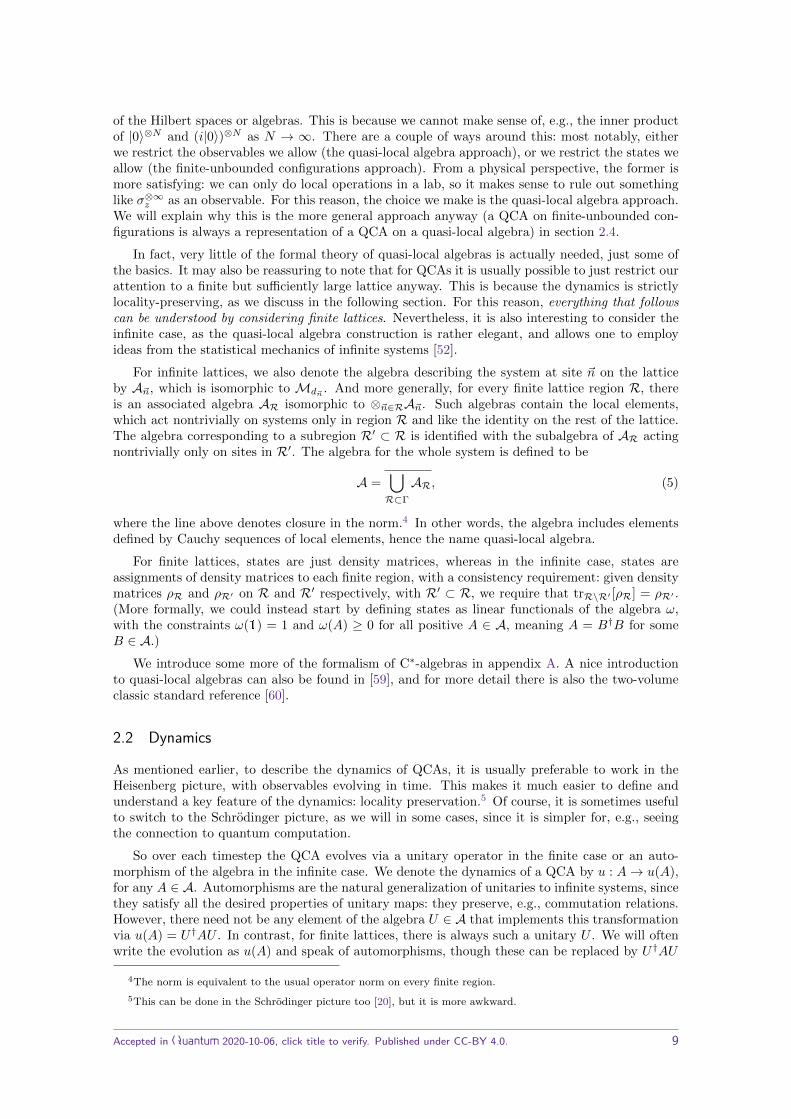
of the Hilbert spaces or algebras. This is because we cannot make sense of, e.g., the inner productof |0〉⊗N and (i|0〉)⊗N as N → ∞. There are a couple of ways around this: most notably, eitherwe restrict the observables we allow (the quasi-local algebra approach), or we restrict the states weallow (the finite-unbounded configurations approach). From a physical perspective, the former ismore satisfying: we can only do local operations in a lab, so it makes sense to rule out somethinglike σ⊗∞z as an observable. For this reason, the choice we make is the quasi-local algebra approach.We will explain why this is the more general approach anyway (a QCA on finite-unbounded con-figurations is always a representation of a QCA on a quasi-local algebra) in section 2.4.

In fact, very little of the formal theory of quasi-local algebras is actually needed, just some ofthe basics. It may also be reassuring to note that for QCAs it is usually possible to just restrict ourattention to a finite but sufficiently large lattice anyway. This is because the dynamics is strictlylocality-preserving, as we discuss in the following section. For this reason, everything that followscan be understood by considering finite lattices. Nevertheless, it is also interesting to consider theinfinite case, as the quasi-local algebra construction is rather elegant, and allows one to employideas from the statistical mechanics of infinite systems [52].

For infinite lattices, we also denote the algebra describing the system at site ~n on the latticeby A~n, which is isomorphic to Md~n . And more generally, for every finite lattice region R, thereis an associated algebra AR isomorphic to ⊗~n∈RA~n. Such algebras contain the local elements,which act nontrivially on systems only in region R and like the identity on the rest of the lattice.The algebra corresponding to a subregion R′ ⊂ R is identified with the subalgebra of AR actingnontrivially only on sites in R′. The algebra for the whole system is defined to be

A =⋃R⊂ΓAR, (5)

where the line above denotes closure in the norm.4 In other words, the algebra includes elementsdefined by Cauchy sequences of local elements, hence the name quasi-local algebra.

For finite lattices, states are just density matrices, whereas in the infinite case, states areassignments of density matrices to each finite region, with a consistency requirement: given densitymatrices ρR and ρR′ on R and R′ respectively, with R′ ⊂ R, we require that trR\R′ [ρR] = ρR′ .(More formally, we could instead start by defining states as linear functionals of the algebra ω,with the constraints ω(1) = 1 and ω(A) ≥ 0 for all positive A ∈ A, meaning A = B†B for someB ∈ A.)

We introduce some more of the formalism of C∗-algebras in appendix A. A nice introductionto quasi-local algebras can also be found in [59], and for more detail there is also the two-volumeclassic standard reference [60].

2.2 Dynamics

As mentioned earlier, to describe the dynamics of QCAs, it is usually preferable to work in theHeisenberg picture, with observables evolving in time. This makes it much easier to define andunderstand a key feature of the dynamics: locality preservation.5 Of course, it is sometimes usefulto switch to the Schrodinger picture, as we will in some cases, since it is simpler for, e.g., seeingthe connection to quantum computation.

So over each timestep the QCA evolves via a unitary operator in the finite case or an auto-morphism of the algebra in the infinite case. We denote the dynamics of a QCA by u : A→ u(A),for any A ∈ A. Automorphisms are the natural generalization of unitaries to infinite systems, sincethey satisfy all the desired properties of unitary maps: they preserve, e.g., commutation relations.However, there need not be any element of the algebra U ∈ A that implements this transformationvia u(A) = U†AU . In contrast, for finite lattices, there is always such a unitary U . We will oftenwrite the evolution as u(A) and speak of automorphisms, though these can be replaced by U†AU

4The norm is equivalent to the usual operator norm on every finite region.5This can be done in the Schrodinger picture too [20], but it is more awkward.


and unitaries respectively for finite systems. Note that u(AB) = u(A)u(B) always, so it is enoughto understand how single-site algebras evolve to understand the whole evolution.

Figure 4: A unitary or automorphism is locality preserving if it maps local operators to local operators (in theHeisenberg picture). At t = 0 an operator A is localized on four sites, but after one timestep the updatedoperator u(A) is localized on nine sites nearby.

We also demand that the evolution is locality preserving (see figure 4). This means that localoperators get mapped to operators localized on a region nearby. Sometimes the locality preservingproperty is called causality (e.g., in [20, 61]) in analogy with relativistic causality. More precisely,we have the following definition.

Definition 2.2.1. The dynamics of a QCA u is locality preserving if there is some range l ≥ 0such that, for any ~n and any operator A localized on ~n, then u(A) is localized on a region consistingonly of sites ~m with |~n− ~m| ≤ l. Here we use the Taxicab metric on the lattice.

We may also define the neighbourhood of a point ~n, which we denote N (~n). Then N (~n) is thesmallest region on which the algebra u(A~n) is localized. We can generalize this to describe theneighbourhood of a region R, denoted by N (R).

We can put all this together to give a summary of the definition of a QCA.

Definition 2.2.2. A QCA consists of a discrete hypercubic lattice, which may be finite or be Zd,with a finite quantum system at each site (qudits and/or fermion modes). Evolution takes placeover discrete timesteps via a locality-preserving automorphism (or unitary for finite systems).

We will not always assume that QCAs are translationally invariant (which means that thedynamics commutes with shifts along any lattice direction), though this was traditionally assumedin many works. Sometimes we will restrict to this case, as further interesting results then follow. Itwould be more in the spirit of classical CAs, to always consider translationally invariant dynamics,but some of the most interesting QCA structure theorems do not require any form of translationalinvariance (see section 5). As an aside, it would also be interesting to consider irreversible (i.e.,nonunitary) QCAs, as in [18, 52, 62], though not much work has been done in this direction. Inthis case, e.g., unitaries would be replaced by completely positive trace-preserving maps, which arethe most general possible dynamics consistent with quantum theory [17]).

Finally, a useful alternative possibility to just fixing a lattice, described in [63], involves controlspaces. In that case, we start with a control space, which is typically a smooth manifold M witha metric d(x, y). The manifold can be unbounded or bounded and with or without boundary. Todefine a QCA we embed the points of a discrete set I, which label lattice sites, into the controlspace via I : I →M. The lattice sites have quantum systems associated to them, and they inherita notion of distance from the metric of the control space.


A family of QCAs is a sequence of QCAs labelled by i ∈ N with control space M with embed-dings Ii. Each QCA has an automorphism ui with range li. And we require that li → 0 as i→ 0,which is because we are now measuring distance with the metric of the control space. So intuitively,if we take some point x, then for larger i the embedding will include more and more points withina fixed distance of x. So we then require that the QCAs’ range, as measured with this distancegoes to zero as i→∞. As an example, the control space could be a circle with circumference one,and the family of QCAs could correspond to finer and finer equally spaced points on the circle,e.g., ui could live on all sites separated by a distance 1/2i on the circle. More interesting examplesof control spaces would be higher dimensional tori or the two-dimensional infinite plane with ahole at the origin.

2.3 Global and local transition rules

As we saw in section 1, in the classical setting, CAs are usually defined by a local transitionrule. This tells us how, e.g., the bit at site n updates its state depending only on the states of itsimmediate neighbours. In the previous subsection, however, we defined QCAs by a global transitionrule—an automorphism or unitary of the observable algebra that preserves locality. However, wemay also specify a QCA by local transition rules [19]. To go from a global rule to local rules, wedefine the local transition rules to be the maps α~n : A~n → AN (~n) such that

α~n(A) = u(A) for any A ∈ A~n. (6)

This α~n tells us how observables localized on ~n spread out in N (~n). (In the translationally invariantcase, it is enough to specify α~0.) To get something closer to the local rules of classical CAs, wecould then switch to the Schrodinger picture, though this description will be quite cumbersome.

In equation (6), we simply defined the local rule by using the global rule, so it is obvious that weget a sensible QCA and that the global dynamics uniquely specifies the local transition rules. Onthe other hand, going the opposite direction is more interesting: we may start with some candidatefor a local rule, some β~n taking A~n to AN (~n) for every ~n. Then we define a candidate for a globalrule v to be linear, and to act on products of operators at different sites in the following way. If Aand B are elements from A~n and A~m respectively,

v(AB) = β~n(A)β~m(B). (7)

Starting from such a local rule, the question is whether this candidate is a bona fide QCA? Forexample, our rule may not be a valid automorphism; it may not even be invertible. The firstcondition we need to ensure that we have a QCA is that β~n must be an isomorphism, so it mustpreserve the algebraic structure locally, mappingA~n to an isomorphic subalgebra ofAN (~n) for every~n (something like β~n(A) = 0 for all A will obviously not do). In fact, the only other condition weneed is that, for any ~n 6= ~m, and any A ∈ A~n and B ∈ A~m,

[β~n(A), β~m(B)] = 0. (8)

These two conditions are enough to guarantee that the map defines an automorphism. This wasproved in [19] for one-dimensional translationally invariant QCAs of qudits, but the proofs carryover straightforwardly to non-translationally invariant and higher dimensional systems.

For non-translationally invariant QCAs, checking that equation (8) holds will usually be im-possible, as we cannot check an infinite number of conditions in practice. On the other hand, fortranslationally invariant systems, because the neighbourhoods are finite, we need only check that[β~0(A), β~n(B)] = 0, for all A ∈ A~0 and B ∈ A~n, when the neighbourhoods of ~0 and ~n overlap,

i.e., N (~0) ∩ N (~n) 6= ∅. And we need only check this for a basis of elements of A~0 and A~n for

each ~n with N (~0) ∩ N (~n) 6= ∅. This means that only a finite number of commutators need to becomputed, making it feasible to check if a local rule indeed gives a legitimate QCA.

In the translationally invariant case, there is also a natural correspondence between QCAson infinite lattices and QCAs on finite lattices, which works because the dynamics is locality


preserving. This is called the wrapping lemma [19]. This means that any translationally invariantQCA on an infinite lattice is in one-to-one correspondence with a QCA on any finite lattice withperiodic boundary conditions (and the same dimension), provided the finite lattice is big enoughthat the overlaps of the neighbourhoods of two sites are the same as for the infinite case. This wasrecently generalized to fermions in [64].

2.4 Finite, unbounded configurations

An alternative way to deal with infinite systems and infinite tensor products (as opposed to thequasi-local algebra approach we use here) constructs a Hilbert space called the Hilbert space offinite, unbounded configurations. This is used, for example, in [65]. As we will see, this is coveredby our definition, as these are always representations of a subset of QCAs defined in our sense.

The idea of the finite, unbounded configurations approach is to restrict the possible states thesystem can be in. We start by assuming that each lattice site can be in one of a finite numberof states, and one of these states is a privileged state, called a quiescent state q. We allow allconfigurations of the system where only a finite number of sites are not in the quiescent state, e.g.,infinite strings like ...q q q a b c q q q... for a one-dimensional system. Then we use these strings tolabel an orthonormal basis of a complex vector space. To get a Hilbert space, we complete thevector space in the inner-product norm. This Hilbert space is separable (i.e., it has a countablebasis) and is sometimes called an incomplete infinite tensor product space. This is the Hilbertspace of finite, unbounded configurations.

Notice that this Hilbert space admits all operators corresponding to the quasi-local algebra ofthe system: we can perform any local operation we like, as this will only change the state in somefinite region and will keep us in the Hilbert space of finite, unbounded configurations. Next wedefine the dynamics to be determined by a locality-preserving unitary U on this Hilbert space. (Weuse the exact same notion of locality preserving as before in this setting, working in the Heisenbergpicture.) Requiring that U is unitary, translationally invariant,6 and locality preserving meansthat U must preserve the state |...qqqqq...〉. The advantage of this formalism is that we can workwith Hilbert spaces and unitaries, instead of algebras and automorphisms. The disadvantage isthat we exclude many interesting states and dynamics on the system (a workaround should bepossible by increasing the local dimension in the finite, unbounded configurations setting). Forexample, the unitary must always have the product state |...qqqqq...〉 as a +1 eigenvector.

Instead of constructing the Hilbert space of finite, unbounded configurations and QCAs onthem in this way, we can construct them as a representation of a QCA defined in the quasi-localalgebra setting. (See [66] for a similar construction in the translationally invariant case.) Supposewe have a QCA with dynamics u, and let ω be some invariant state, so ω(u(A)) = ω(A) for allA ∈ A. Here we are writing the expectation value of A in state ω as ω(A) (for finite systems,this would be tr[ρA] for some density operator ρ). We can always construct a representation ofthe algebra where the state ω is represented in the resulting Hilbert space H by a normalizedvector |ω〉, with the representation of any operator A being denoted π(A). (This uses the GNSrepresentation of the algebra, which is described in appendix A.) Furthermore, because u leaves thestate ω invariant, there is a unique unitary U that implements the dynamics in the representation,i.e., U†π(A)U = π(u(A)) and U |ω〉 = |ω〉 (see appendix A and [60]). To connect with the finite,unbounded configurations approach, let us suppose that ω is a pure product state. Then therepresentation π(A) is irreducible. We can construct an orthonormal basis for H by applying localoperators π(A) to |ω〉, and because the Hilbert space must be complete, we get exactly the Hilbertspace of finite, unbounded configurations. As an example with qubits on a line, we could choose ωto be the 0 state of all the qubits. In the representation, we would have |ω〉 = |0...000...0〉. Then, forexample, the action of the Pauli X operator at site n is given by π(Xn)|0...000...0〉 = |0...010...0〉.An example of a QCA dynamics leaving ω invariant is the CNOT QCA in section 1.1.

We should emphasize that any QCA defined in the finite, unbounded configuration picturecan be expressed in our formalism, as an automorphism on the quasi-local algebra. This follows

6This is usually but not always an assumption in the finite, unbounded configurations setting.


because the unitary implementing the dynamics for a finite, unbounded configuration also definesan automorphism of the algebra of local operators that is locality-preserving and hence uniquelydefines dynamics for a QCA in the quasi-local algebra picture. So the finite, unbounded configur-ations QCAs can be viewed as special cases of our notion of QCAs. But for some applications, itis useful and intuitive to use the finite, unbounded configurations picture.

To see that there are QCAs that cannot be expressed in terms of a Hilbert space of finite,unbounded configurations (at least without adding local ancillas), consider that a translationallyinvariant QCA need not have any invariant pure product state, something which we would actuallyexpect to be the case in general. If this is the case, then it is not directly representable in the finite,unbounded configuration picture. As quantum field theories, for example, have highly entangledvacua [67], it seems clear that any ideas for discretizing such models with QCAs would not benaively representable by finite, unbounded configurations.

The finite, unbounded configurations approach to QCAs was used as a definition of a Schrodingertemplate of a QCA in [66]. We can easily generalize this by constructing a representation of thequasi-local algebra and dynamics using any invariant state (not necessarily a product state) of theautomorphism as described above. Then one has a picture of the QCA with a Hilbert space ofstates and dynamics represented by a unitary. Indeed, it seems reasonable to view the invariantstate in that case as a vacuum state and to think of the resulting Hilbert space as the space oflocalized excitations above the vacuum state. From that point of view, it would make sense tocall the resulting Hilbert space the Hilbert space of finite, unbounded excitations. And so we couldinterpret the main result of [66] as characterizing when a QCA admits a representation in termsof finite, unbounded configurations with an invariant product state.

3 More examples of QCAs

There are several different specialized classes of QCAs that fit into our framework. We will lookat two below. The first class of QCAs involve applying shifts and local unitary circuits. Thesetypically involve some kind of partitioning scheme for the lattice. Such QCAs have been particularlyimportant, as they are manifestly unitary and have been used to show universality of QCAs forquantum computation [16]. Some discussions of the different models can also be found in [19, 46,68]. The second class of QCAs that we will discuss are Clifford QCAs. In this case, we restrict todynamics that map strings of generalized Pauli operators to strings of generalized Pauli operators.In contrast to the first class of QCAs, which are constructive by their definition, Clifford QCAs,are defined by a constraint on their dynamics, but it is this restriction makes this class of QCAstractable.

3.1 Partitioning schemes

In section 1.1 we saw two examples of QCAs: constant-depth circuits and shifts. These basicbuilding blocks can be combined to get various different classes of QCAs that appear in theliterature.

As a first step, we can generalize the finite-depth circuit QCA construction from section 1.1 inthe following way.

Definition 3.1.1. Finite-depth circuit QCA: Consider P different partitions of the lattice intosupercells Cp~n, with ~n ∈ Zd and p ∈ 1, ..., P. This is done in such a way that, for each partition,each cell on the lattice is contained in exactly one supercell (see figure 5). Then the dynamics isgiven by

u1 ... uP , (9)where each up is a product of unitaries Up~n localized on Cp~n. In other words,

up(·) =(∏

~n

Up†~n

)·

(∏~n

Up~n

), (10)


Figure 5: To define QCA dynamics it is often useful to partition the lattice into supercells by grouping sitestogether. (The supercells can have any shape as long as they are finite.) Then we apply unitaries to eachsystem in the supercells. More generally we consider several different partitions and apply different unitaries tosupercells in each partition in sequence to implement the QCA dynamics.

where the order in the products does not matter because the unitaries act on non-overlapping regionsand hence commute.

As an example of QCAs using such a partitioning scheme, let us look at the block-partitionedQCAs defined in [18], which use layers of conditional unitaries. In the nearest-neighbour case withqubits on a one-dimensional system, we define the operator (acting nontrivially on sites n − 1, nand n+ 1 only)

Dabn = |a〉〈a|n−1 ⊗ vabn ⊗ |b〉〈b|n+1, (11)

where a, b ∈ 0, 1 and vabn is a unitary on site n. Then we can define the conditional unitaryoperator

Vn =∑

a,b∈0,1

Dabn . (12)

If the qubits n + 1 and n − 1 are in, e.g., the 0 state, this implements the unitary v00 on qubitn. The QCA dynamics is then given by a depth-three circuit: first we apply Vn to all cells withn mod 3 = 0, then to all cells with n mod 3 = 1, and finally to all cells with n mod 3 = 2. Thisway unitaries are never applied simultaneously on overlapping supercells.

The properties of these QCAs were studied in [18], where information transport along the lineand entanglement generation were studied. This partitioning scheme also makes the constructionof non-unitary QCAs straightforward [18], by replacing the local unitaries by local completelypositive trace-preserving maps. This allows one to construct an irreversible QCA that gives aquantum version of the classical rule 110 CA from section 1. To see that we need a non-unitaryQCA to do this, notice that rule 110 itself is irreversible. This can be seen by considering the statewith 0 everywhere and the state with 1 everywhere. After one timestep, these both get mappedto the same state.

We can also generalize the shift along a line to shifts along lattice directions for higher dimen-sional systems. Suppose the lattice has lattice basis vectors ~ei where i ∈ 1, ..., d, then we definethe shift along lattice direction ~ei by

si(A~n) = A~n−~ei , (13)

which has no other effect than to shift the algebra by one step in the direction ~ei. We may alsoconsider partial shifts. These would just shift a subalgebra instead of the whole algebra. Oneuseful example involves a one-dimensional lattice with qudits at each site. Then we divide the cellsinto three subcells, which we label by l, c and r. So we may write An = Bln ⊗ Bcn ⊗ Brn. Then wedefine the conditional shift σ to be

σ(Bln) = Bln+1

σ(Bcn) = Bcnσ(Brn) = Brn−1.

(14)


This particular conditional shift (we could define more general versions, particularly in higherlattice dimensions) is useful for constructing the partitioned QCAs in [16, 31], which are usuallyreferred to as Watrous partitioned QCAs. After applying σ, we may also apply an automorphismλ that is just a product of on-site unitaries. The overall dynamics is as illustrated in figure 6. Itis easy to see then that the dynamics is an automorphism. Interestingly, this is a special case ofquantum lattice gas automata, which we will return to in section 6.4.1. These comprise partialshifts (which are interpreted as propagating different particle types on the lattice) and on-siteunitaries (which model interactions between particles).

Figure 6: A Watrous QCA shifts some subsystems left and some right while some remain stationary eachtimestep. On-site unitaries also get applied before or after the shift step. Each site has three qudits, representedby yellow boxes: Bln, Bcn and Brn.

Other examples of QCAs defined via partitioning schemes arise in the literature, e.g., localunitary QCAs [53]. As an aside, it is worth pointing out that many of these partitioning schemeswere initially introduced in the framework of finite, unbounded configurations, but they also fitperfectly well into our framework.

All examples in the section fall into a class of QCAs called trivial [27].

Definition 3.1.2. A QCA u is trivial if, possibly by adding ancillary degrees of freedom at eachlattice site, we can decompose u⊗1 into a finite-depth circuit QCA followed by some shifts, where1 acts on the ancillary degrees of freedom.

Of course, the word trivial underplays the importance of such QCAs, as most of the interestingexamples of QCAs that we will see are trivial. On the other hand, this makes nontrivial QCAs,which we will return to in section 6.3, all the more interesting.

3.2 Clifford QCAs

An important class of QCAs are Clifford QCAs [19]. Such models are efficiently classically sim-ulatable, so Clifford QCAs cannot be universal for quantum computation (except in the unlikelyevent that quantum computers can be efficiently classically simulated). Nevertheless, they haveinteresting properties, practical uses, and provide a nice playground to get some intuition aboutQCA dynamics.

Definition 3.2.1. Clifford QCAs are defined on lattices of qubits or qudits, where the dynamics isa Clifford operation, which means it takes any product of (generalized) Pauli operators to a multipleof a product of (generalized) Pauli operators. (Generalized Pauli operators are defined below.)

Here we will mostly consider one-dimensional translationally invariant Clifford QCAs on qubits.Let us look at an example of such a Clifford QCA from [19]. The dynamics are determined by theautomorphism ul acting as

ul(Xn) = Zn

ul(Zn) = Zn−l ⊗Xn ⊗ Zn+l,(15)


for a fixed l ∈ Z. Notice that this already determines the dynamics completely because ul(AB) =ul(A)ul(B) and ul is linear. For example, with l = 1 and writing u = u1, we can easily calculateu(Y0 ⊗ Z3) to get

u(Y0 ⊗ Z3) = u(Y0)u(Z3)= iu(Z0)u(X0)u(Z3)= −Z−1 ⊗ Y0 ⊗ Z1 ⊗ Z2 ⊗X3 ⊗ Z4,

(16)

where the last line follows from equation (15).

The Clifford constraint is quite strong, and as a result to understand the dynamics we need onlylook at a CA. Let us see how this works for the example above. We can represent Pauli productsby strings of integers. We label 1, X, Y, Z by 0, 1, 2, 3 respectively. Given an initial string of Paulis,we represent it by a string µ = (..., µ−1, µ0, µ1, ...), where µm ∈ 0, 1, 2, 3 for each m ∈ Z. To findout the value of the string at position m = 0 after one timestep we need only know µ−1, µ0 andµ1. Suppose, e.g., we have (..., µ−1, µ0, µ1, ...) = (..., 2, 1, 2, ...), which represents an operator thathas the form A−∞,...,−2⊗ Y−1⊗X0⊗ Y1⊗B2,...,∞, where A−∞,...,−2 and B2,...,∞ are someproducts of Paulis on the rest of the qubits. After one timestep we have

u(A−∞,...,−2 ⊗ Y−1 ⊗X0 ⊗ Y1 ⊗B2,...,∞

)= A′−∞,...,−1 ⊗ Z0 ⊗B′1,...,∞ (17)

by using equation (15), and A′−∞,...,−1 and B′1,...,∞ are strings of Paulis now localized on regions

−∞, ...,−1 and 1, ...,∞ respectively. Thus, we get µ′0 = 3 after the update. By finding µ′0 forall possible products of Paulis on the sites −1, 0, 1, we infer the corresponding CA rule. In thiscase, the CA consists of a discrete line of cells where each cell has four possible states in 0, 1, 2, 3,and the update rule for a site depends only on its nearest neighbours. Note that we disregardthe overall phase: a Clifford operation could map, e.g., Xn to −Xn, but we ignore this. This CAdescription is enough to tell us how strings of Paulis spread out. An example of the dynamicsof the ensuing CA is shown in figure 7. In [69, 70], far more sophisticated methods are used forstudying Clifford QCAs, but we can already understand a lot of the structure by deriving CAs forthe evolution of Pauli strings as we have done here.

Figure 7: An example of Clifford QCA dynamics with update rule fully specified by Xn → Xn−1 ⊗ Yn ⊗Xn+1and Zn → Xn. Each square represents an element in a Pauli string: white represents 1, X is yellow, Y is blueand Z is green. Notice the fractal structure in the spacetime diagram (where time goes up).

Furthermore, Clifford QCAs on a line can be classified into three classes [70, 71]. There arethose with gliders, which are observables that simply move along the line each timestep; there areperiodic Clifford QCA, which are periodic in time; and there are fractal Clifford QCA, which areself similar on large scales of a spacetime diagram, an example of which can be seen in figure 7.The QCA in equation (15) with l = 1 has examples of gliders. Consider the observable X0 ⊗ Z1.


After one timestep, this is mapped to u(X0 ⊗ Z1) = X1 ⊗ Z2, so it is just translated to the right.Similarly, Z0 ⊗ X1 gets translated to the left by the QCA. The fractal structure in spacetimeplots of fractal Clifford QCAs was studied in further detail in [71, 72]. This was made possible byanalysing the resulting fractal structures in the corresponding CAs.

Additionally, entanglement generation in Clifford QCAs was studied in [70, 71]. In [69], itwas also shown that every unique translationally invariant stabilizer state in one dimension canbe generated by the action of a Clifford QCA acting on a product state. And Clifford QCAsplay a role in understanding the properties of stabilizer codes in more general systems [73]. Morerecently, the eigenstates of Clifford QCAs have been analysed in [74], where it was seen that theeigenstate thermalization hypothesis does not apply to these models. The eigenstate thermalizationhypothesis is the hypothesis that, when we look at the reduced state of an energy eigenstateon a small subsystem, we approximately get a thermal state with a temperature that does notvary too quickly with the energy of the eigenstate. (There are a few different versions of theeigenstate thermalization hypothesis, and this is just one of them.) On the one hand, it may notbe so surprising that Clifford QCAs, which are discrete-time systems with a lot of structure, donot satisfy the eigenstate thermalization hypothesis. But on the other hand, there is evidencethat periodically driven Hamiltonian systems satisfy the hypothesis [75], and QCAs are a usefulapproximate model for such systems, something we will discuss further in section 6.1.

As we just saw, the constraint that the evolution is a Clifford operation is quite powerful, andthe simplification arising from this constraint can be generalized [69]: one can go beyond qubitsand Pauli operators, instead looking at p dimensional qudits and discrete Weyl operators, providedp is prime. Fixing an orthonormal basis for such a qudit to be |q〉, with q ∈ 0, ..., p− 1, then theWeyl (or generalized Pauli) operators, which generalize X and Z, are defined by

X|q〉 = |q + 1〉Z|q〉 = e2πiq/p|q〉,

(18)

where the addition in the first line is defined modulo p. Again we have the constraint that productsof Weyl operators, e.g., Xn⊗Zn+1 get mapped to products of Weyl operators. Many of the resultsfor qubit systems extend to these systems, though at the cost of being a bit more complicated [69].

Remarkably, the QCAs in equation (15) for different values of l, together with on-site Cliffordoperations and the shift generate all possible translationally invariant qubit Clifford QCAs in onedimension [69]. And much of the general structure of qudit Clifford QCAs has been understoodrecently in [76], where it was shown that the fourth power of any translationally invariant CliffordQCA is trivial, in the sense that it can be decomposed into a constant-depth circuit followed byshifts. Instead of the Clifford constraint, we could just restrict the QCA neighbourhood and thedimension of the systems at each site. This was done in [19], where it was shown that nearest-neighbour qubit QCAs are always decomposable in terms of shifts, on-site unitaries and controlledphase gates. Furthermore, in two dimensions every QCA is known to be trivial [63, 76], a fact thatwas already known in one dimension as a consequence of index theory [77].

4 QCAs as quantum computers

QCAs were originally envisaged as a model of quantum computation, useful for simulating physicsor implementing more general quantum algorithms. One of the earliest breakthroughs in this regardwas the proof that QCAs can efficiently simulate quantum Turing machines with only constantslowdown [16]. The proof used the Watrous partitioned QCAs of the previous section.

If we consider instead the circuit model of quantum computation, it is clear from a result that wewill see in section 5.1 that the circuit model can efficiently simulate any QCA.7 And we know thatthe converse is true because we can use a QCA to simulate a quantum Turing machine, which can

7Of course, another way to see this is by using a quantum circuit to simulate a quantum Turing machine [78] thatin turn simulates a QCA. This would work in one dimension at least, since quantum Turing machines can simulatethese Watrous partitioned QCAs with linear slowdown [16].


then simulate the circuit model. Nevertheless, it will be interesting to look at an explicit examplein the following section where we directly simulate a quantum circuit with a QCA. Note that weonly consider translationally invariant QCAs in this section. (Relaxing this constraint would makethe results trivial. Besides, the main appeal of quantum computation via QCAs is that ideally oneneed only apply global operations without worrying about implementing many different single- orfew-qubit operations. This advantage may be lost in the translationally non-invariant case.)

4.1 A QCA efficiently simulating quantum circuits

Let us look at a prescription from [79] for simulating quantum circuits using a translationallyinvariant QCA on a finite lattice. The QCA system is a two-dimensional discrete torus (i.e., atwo-dimensional lattice with periodic boundary conditions), and the program itself, as well as theinput data for the algorithm, are encoded in the initial state of the QCA. In this section it will bemore convenient to work in the Schrodinger picture.

We label the sites of the torus with coordinates ~n ∈ 0, ..., 2s − 1 × 0, ..., 2r − 1, and eachsite has a single qubit. We label columns on the torus by the second component of ~n, which rangesfrom 0 to 2r − 1. The qubits in the odd-numbered columns will encode what gates we wish toimplement. So for the purposes of the algorithm, these qubits will always be in one of the the twocomputational basis states |0〉 and |1〉. The qubits on the even-numbered columns will encode thedata that our quantum circuit is to act upon. In particular, at time t = 0 column 0 has the initialinput data for the quantum algorithm.

Figure 8: The two different partitions used to define the QCA are 2× 2 squares as shown in subfigure (a). Thefirst is given by the squares with solid red lines (with upper left site having both coordinates even, e.g., (0, 0)),and the second corresponds to the green boxes with dotted lines (with upper left site having both coordinatesodd). Subfigure (b) shows the simpler labelling of qubits in one of the supercells used to define the unitary inequation (20).

We will use the supercell partitioning scheme of section 3.1, with two simple partitions of thetorus, but we will consider the application of the unitaries to both partitions to correspond to twotimesteps, meaning the evolution is different for even and odd timesteps. The partitions are asshown in figure 8 (a). The first consists of 2× 2 squares of cells with the cell in the top left cornerhaving both coordinates even, e.g., ~n = (0, 0). The second consists of 2×2 squares of cells but nowwith the cell in the top left corner having both coordinates odd, e.g., ~n = (1, 1). So the supercellsin the first partition are labelled by vectors with both components even, and those in the secondpartition are labelled by vectors with both components odd.

Next we define the unitaries that act on these supercells, which all have the same form:

V~n = S~nW~n, (19)

where S~n just swaps the states of the two left qubits in the square with the two qubits on the right.This part of the gate swaps the data qubits with the program qubits after applying W~n. To makethe notation simple, label the four sites as in figure 8 (b). For W we take

W = H1C3[U1]C4[R12]. (20)

Let us go through each of the components on the right hand side. Two of these unitaries arecontrolled by the program qubits: C3[U1] and C4[R12] are unitaries applied to data qubits controlled


by the program qubits 3 and 4. So if, e.g., qubit 3 is in the |1〉 state, the unitary U1 is applied toqubit 1, and if it is in the |0〉 state, the identity is applied. H1 is the Hadamard gate applied toqubit 1, i.e., H1 = (X1 + Z1)/

√2. The choice made in [79] for the gates U1 and R12 is

U1 = exp(−iπ8Z1

)R12 = C1[Z2],

(21)

so R12 is simply a Pauli Z operator on qubit 2 controlled on qubit 1. (These are both data qubits.)

The evolution at even and odd timesteps is then given by the products

Veven =∏

~n even

V~n

Vodd =∏~n odd

V~n,(22)

where the product in the first/second line is over all ~n with both entries even/odd. Now considerthe initial state

|ψ(0)〉 =r−1⊗i=0|Di(0)〉2i|Pi+1〉2i+1. (23)

Here |Di(0)〉2i is the state of the data qubits in column 2i. And |Pi+1〉2i+1 is the state of the qubitsin column 2i+ 1, which encode the program, i.e., the unitaries that should be implemented on thedata qubits by the dynamics. Note that the subscript label on the kets denotes the column wherethe qubits are, whereas the subscript label within the qubits specifies the state. Let us use [m]kto denote m modulo k. After t timesteps, the state is given by

|ψ(t)〉 =r−1⊗i=0|Di(t)〉[2i+t]2r ⊗ |P[i+t+1]r 〉[2i+t+1]2r , (24)

where, in particular,|D0(t)〉 = G(Pt)...G(P1)|D0(0)〉, (25)

where G(Pi) are unitaries composed of the gates applied at each timestep as the input data columnmoves across the torus encountering new program qubits. The other vectors |Di(t)〉 in equation(24) with i 6= 0 will have unitaries G(Pi) applied in some other order, but this is unimportant, aswe are only interested in implementing the quantum algorithm on the input data that started att = 0 in the first column. And to do this, we encode the necessary gates into the program qubitsPi. For example, G(P1) is given by∏

n1 evenn2=0

W~n|D0(0)〉0|P1〉1 = G(P1)|D0(0)〉0|P1〉1. (26)

Note that the product above only involves unitaries on the first two columns. Recall from earlierthat these W~n unitaries were specifically chosen to implement desired gates on the data qubitscontrolled on the program qubits.

After r timesteps (any longer and the data qubits encounter program qubits twice) the outputof the program can be read from column r. It was shown in [79] that with this setup, the choice ofgates in equation (21) is sufficient to implement a universal gate set on the data qubits and hencesimulate any quantum circuit efficiently.

A similar idea was used in [53], where again the circuit to be simulated is, in a sense, drawnonto a two-dimensional QCA.

4.2 Other ideas

A drawback of the method of the previous section, which maps the circuit onto a two-dimensionalQCA, is simply that it is two dimensional. This may be difficult to do in a laboratory, so it


may be more desirable for practical reasons to work with a one-dimensional QCA. That quantumcircuits can be efficiently simulated by a one-dimensional QCA was shown in [80], which gave aconstruction for a universal one-dimensional QCA with 12 dimensional quantum systems at eachcell. A stepping stone to get this result was a proof that QCAs with external classical control canbe simulated by those without. In this context, a classically controlled QCA is a QCA where anexternal party can choose to evolve the system via one of some number of automorphisms at eachtimestep. (This is also sufficient for quantum computation [81].) By encoding which automorphismis to be applied at each timestep into the initial state, it is possible to get a truly autonomousQCA [80], albeit with a bigger state space.

An interesting related concept to the quantum computational universality we are interested inhere is so-called intrinsic universality. For QCAs this amounts to finding a QCA that, after someregrouping of cells, can simulate any other QCA. This has been studied in detail in [82–85], wheren-dimensional intrinsically universal QCAs were found [83, 84].

One might speculate on the possibility of using fermionic QCAs as quantum computers insteadof qudit QCAs. This would be a QCA analogue of using fermionic quantum circuits for quantumcomputation instead of qubit circuits [86]. (Also, the opposite direction, simulating fermionicsystems with qubit quantum circuits, is highly relevant for quantum simulations of physics [87].)For the quantum circuit model, it was shown in [86] that quantum computers using qubits canefficiently simulate quantum computers composed of fermions and vice versa. A similar resultis true for QCAs: fermionic QCAs can simulate qudit QCAs efficiently and vice versa directly(without, e.g., simulating the circuit model first) [57]. In this case, the slowdown is constant inboth directions.

4.3 Implementations

In contrast to the circuit model of quantum computing, which uses single and (typically) fewqubit gates to build a global unitary circuit, quantum cellular automata involve global unitaryoperations, without necessarily requiring the ability to directly apply, e.g., single-qubit gates. Thisis often put forward as an advantage because single-site addressability can be harder in practice[88].

One interesting possibility, first proposed in one of the earliest papers on QCAs [15], is toarrange three types of atomic species periodically in an ...ABCABC... pattern. Each species canbe addressed independently with electromagnetic pulses tuned to have the resonant frequency of aspecies’ ground to excited state transition. (Note that for each atom, the resonant frequency canbe affected by the states of its neighbours, which is a useful feature in the proposal as it allows,e.g., conditional operations to be implemented.) With various different combinations of pulses,one can implement various different gates. The input and readout of data occurs only on the endqubits of the line. Later it was shown in [88] that two species in an ...ABAB... pattern sufficesfor universal quantum computation. (In fact, even a single species should be sufficient [81, 89].)These kinds of models are what some authors mean by the name quantum cellular automata (e.g.,in [90]), whereas, from our point of view, a better name would be classically controlled QCAs, asthey typically involve different unitaries applied at each timestep.

This scheme was studied further in [91, 92], and in [93] an implementation of this idea usingendohedral fullerenes was analyzed theoretically. Endohedral fullerenes are C60 fullerenes (theseare molecules made of 60 carbon atoms that form a ball, sometimes called buckyballs) that have,e.g., an atom trapped inside the cage formed by the carbon atoms. And the idea of using thesemolecules as parts of a quantum computer met with a degree of experimental success in [94]. Inthat case, Nitrogen atoms were trapped in the fullerenes and the levels considered arose from aspin 3/2 electron coupled to 14N nuclear spin I = 1.

Most recently, a proposal has been made to use ultracold atoms excited to Rydberg states toimplement QCAs in practice [95]. There it was also shown that such QCAs would be well suitedto variational quantum optimization as well as quantum state engineering, which works by tuningthe QCA to get steady states that have a high degree of entanglement.


While quantum computing via quantum cellular automata has its advantages (only globaloperations are necessary), the vast majority of work regarding quantum computing is focussedon other models, especially the circuit model. Perhaps because of this, there is, e.g., no well-developed theory of error correction in quantum cellular automata, in contrast to the quantumcircuit model. (It may be straightforward to develop such a theory, and it would be interestingto see if it could be done without requiring few-qubit operations.) Furthermore, the current trendin building quantum computers is oriented towards quantum computers with a focus on few-qubitaddressability in order to use the quantum circuit model.

5 Structure of QCAs

There are many results that allow one to understand the structure of QCA dynamics. In onedimension, QCAs are particularly well understood. For example, the index theory (discussed insection 5.2) classifies when two QCAs can be smoothly deformed into one another while preservinglocality. In two dimensions, all qudit QCAs can be classified in terms of indices and the topologyof the underlying space, as discussed in section 5.3. And in any dimension, a powerful result isgiven in the following section, where we see that QCAs, together with some local ancillas, allow usto view any QCA as a local finite-depth circuit. Finally, QCAs can be viewed as tensor-networkoperators, something we will see in section 5.6.

5.1 Unitarity plus causality implies localizability

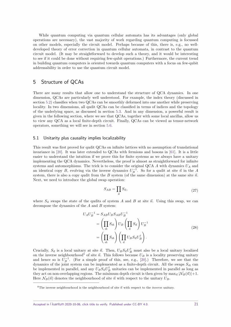
This result was first proved for qudit QCAs on infinite lattices with no assumption of translationalinvariance in [20]. It was later extended to QCAs with fermions and bosons in [61]. It is a littleeasier to understand the intuition if we prove this for finite systems as we always have a unitaryimplementing the QCA dynamics. Nevertheless, the proof is almost as straightforward for infinitesystems and automorphisms. The trick is to consider the original QCA A with dynamics UA andan identical copy B, evolving via the inverse dynamics U−1

B . So for a qudit at site ~n in the Asystem, there is also a copy qudit from the B system (of the same dimension) at the same site ~n.Next, we need to introduce the global swap operation:

SAB =∏~n

S~n, (27)

where S~n swaps the state of the qudits of system A and B at site ~n. Using this swap, we candecompose the dynamics of the A and B system:

UAU−1B = SABUBSABU

−1B

=(∏

~m

S~m

)UB

(∏~n

S~n

)U−1B

=(∏

~m

S~m

)(∏~n

UBS~nU†B

).

(28)

Crucially, S~n is a local unitary at site ~n. Then, UBS~nU†B must also be a local unitary localized

on the inverse neighbourhood8 of site ~n. This follows because UB is a locality preserving unitaryand hence so is U−1

B . (For a simple proof of this, see, e.g., [20].) Therefore, we see that thedynamics of the joint system can be implemented as a finite-depth circuit. All the swaps S~m canbe implemented in parallel, and any UBS~nU

†B unitaries can be implemented in parallel as long as

they act on non-overlapping regions. The minimum depth circuit is then given by max~n |NB(~n)|+1.Here NB(~n) denotes the neighbourhood of site ~n with respect to the unitary UB .

8The inverse neighbourhood is the neighbourhood of site ~n with respect to the inverse unitary.


The result was also later generalized to dynamical graphs in [96], where the QCA neighbourhoodscheme could change over time. This was done with a view towards discrete models of quantumgravity, where spatial geometry may not be fixed in time.

5.2 Index theory in one dimension

In the following sections, we discuss the index for one dimensional QCAs, introduced for quditsin [77]. This was inspired by an analogous index for quantum walks [77, 97], which was called theflow in [97]. Essentially, the index is a number that quantifies how much quantum informationmoves along the line. Interestingly, the QCAs considered need not be translationally invariant, yetone can still assign an index to them. A key property of the index is that it can be computed byexamining the dynamics locally (on a few sites), as we will see. For qudits, the index is a non-zerorational number, whereas interestingly for fermions the index is a non-zero rational number timesa power of

√2. In a very rough sense, the index is determined by how much of a local algebra

of operators (any local algebra corresponding to two or more contiguous sites) of the QCA movesto the left at each timestep. The details are spelled out more precisely in the next few sections,though this requires a few definitions in order to write down a formula that is comprehensible.

5.2.1 Qudit index theory

We first need to introduce a few concepts to define the index. In this section, we assume that theQCAs are nearest neighbour QCAs, which we can always achieve by regrouping sites. Regroupingworks by grouping together sites on the original lattice into a single site on a new lattice. Forexample, we could regroup by defining Bn = A2n ⊗A2n+1 for all n for a one-dimensional system.Then Bn are the cell algebras for the new regrouped system, each of which contain two cells of theoriginal system.

Let us start by introducing support algebras [19, 98]. The intuition underlying support algebrasis that they describe, in some sense, the extent to which one algebra has overlap with anotheralgebra. Note that, for most of our purposes, these algebras are finite dimensional and so areequivalent to matrix algebras.

Definition 5.2.1. Let A, B1 and B2 be C*-algebras, with A ⊆ B1 ⊗ B2. We denote the supportof A in B1 by S(A,B1). This is defined to be the smallest C*-subalgebra in B1 needed to buildelements of A. More concretely, for any a ∈ A, we can decompose it as a =

∑ij b

1i ⊗ b2j , where

b1i ∈ B1 and b2j ∈ B2. Then S(A,B1) is generated by all b1i arising in this way.

Two algebras A and B commute if each element a ∈ A and each element b ∈ B commute. Ifthis is the case, we write [A,B] = 0. The following lemma (see, e.g., [77] for a simple proof) is auseful result, which shows that, if two algebras commute, their support algebras also commute.

Lemma 5.2.2. Suppose we have the C*-algebras B1, B2 and B3. Let A12 and A23 be subalgebrasof B1 ⊗ B2 ⊗ B3 satisfying

A12 ⊆ B1 ⊗ B2

A23 ⊆ B2 ⊗ B3.(29)

Then [A12,A23] = 0 implies[S(A12,B2),S(A23,B2)] = 0. (30)

Another tool we need are the so-called even and odd algebras, which are defined to be

R2n = S (u (A2n ⊗A2n+1) , (A2n−1 ⊗A2n))R2n+1 = S (u (A2n ⊗A2n+1) , (A2n+1 ⊗A2n+2)) .

(31)

These are best understood by looking at figure 9.


Figure 9: Visualization of even and odd algebras. Note that, e.g., R2n rarely equals A2n−1 ⊗A2n.

Recall that An is the algebra at lattice site n. So after evolving A2n ⊗A2n+1 by u, the imageu(A2n ⊗ A2n+1) is a subalgebra of R2n ⊗ R2n+1. These even and odd algebras roughly describewhat information moves right and what information moves left along the line. Next, we need thefollowing important result about the even and odd algebras.

Lemma 5.2.3. Each Rm satisfiesRm 'Mrm , (32)

which is the algebra of rm × rm complex matrices. Note that rm and hence the size of the algebradepends on the position m. Furthermore,

R2n ⊗R2n+1 = u(A2n ⊗A2n+1). (33)

This is proved in, e.g., [77]. We see from equation (33) that

dim[R2n]dim[R2n+1] = dim[A2n]dim[A2n+1], (34)

where dim[·] denotes the dimension of the algebras as vector spaces. Also, we haveR2n+1⊗R2n+2 =A2n+1⊗A2n+2, which follows because the R algebras generate the full system’s algebra, and R2n+1and R2n+2 are the only ones that have support on sites 2n+ 1 and 2n+ 2. Then we get

dim[R2n+1]dim[R2n+2] = dim[A2n+1]dim[A2n+2]. (35)

We may then define the index of a QCA to be

ind[u] =

√dim[R2n]dim[A2n] , (36)

which we can see from equations (34) and (35) is actually independent of n. And because An isisomorphic to Mdn and Rm is isomorphic to Mrn , we get the equivalent formula

ind[u] = r2n

d2n. (37)

(Note that some authors define the log of ind[u] to be the index.)

Let us consider some examples. When each cell of the QCA has a quantum system of the samedimension, a possible dynamics is given by a shift s. When we have d-dimensional qudits at eachsite, it follows from equation (37) that ind[s] = d. If instead we had a shift to the left, given bys−1, then we get ind[s−1] = 1/d. Another interesting choice of dynamics is a local finite-depthcircuit QCA. These always have index ind[u] = 1.

Below we list some basic properties of the index. These are proved in [77], where most prop-erties follow straightforwardly from the definition of the index in equation (37). However, the lasttwo highly interesting properties of the index listed below are harder to prove and tell us somethingabout its robustness with respect to perturbations of the dynamics.

Properties of the index


1. The index ind[u] is locally computable and independent of how we regroup/block sites.

2. The index is a group homomorphism from the group of locality-preserving automorphisms(QCAs) to the group of strictly positive rationals Q+. The identity automorphism getsmapped to 1, and ind[uv] = ind[u] ind[v].

3. The index is multiplicative under tensor products: ind[u⊗ v] = ind[u] ind[v].

4. ind[u] = 1 if and only if u is locally implementable with

u = w v

v(·) =(∏n∈Z

V †2n

)·

(∏m∈Z

V2m

)

w(·) =(∏k∈Z

W †2k+1

)·

(∏l∈Z

W2l+1

),

(38)

where V2n are unitaries acting on sites 2n and 2n + 1, and W2m+1 are unitaries acting onsites 2m + 1 and 2m + 2. So u is a finite-depth circuit. This need not be translationallyinvariant.

5. Two QCAs u0 and u1 with the same C*-algebras (i.e., the same cell structure) have the sameindex if and only if one can be continuously deformed into the other. This means that thereexists a strongly continuous9 path ut with t ∈ [0, 1] connecting u0 to u1 such that ut areQCAs with the same cell structure and neighbourhoods as u0 and u1.

Property (2) and (4) together tell us that applying additional local unitaries cannot change theindex, e.g., ind[u] = ind[v u], where v(·) = V †(·)V for some local V . Property (5) tells us thatsmooth deformations (in terms of the strong operator topology) also cannot change the index, so itis robust against these two types of perturbations. This robustness to perturbations is importantin the application of the index to classifying chiral Floquet phases (section 6.2).

5.2.2 Another formula for the index

There is a different formula for the index which is quite useful [77]. To write it down, we needanother method for quantifying the overlap of two algebras. The algebra of the whole QCA A hasa normalized trace, i.e., a state τ , such that

τ [1] = 1τ [AB] = τ [BA],

(39)

where A,B ∈ A. This state is essentially just the maximally mixed state but for an infinite line.For any A,B ∈ A, τ(A†B) defines an inner product. Because A is a complex vector space, wecan think of any two subalgebras B1, B2 as vector subspaces of A. This allows us to quantify theoverlap of these two subspaces. We pick orthonormal bases for B1 and B2, and denote them by eαand fβ respectively. Then we define the overlap of the algebras to be

η(B1,B2) =√∑

αβ

(τ [e†αfβ ]

)2, (40)

which is independent of the choice of orthonormal bases. We can also think of this as

η(B1,B2) =√

tr[P1P2], (41)

9Strong continuity means that, for any strictly local A ∈ A, ut(A) is continuous in the norm of the C*-algebra.


where P1 and P2 are the projectors onto the subspaces B1 and B2. The trace here is the trace ofoperators on A viewed as an inner product space.10 Note that η(B1,B2) ≥ 1 if both subalgebrascontain the identity.

To get our second formula for the index, define

AL = An−N ⊗ ...⊗AnAR = An+1 ⊗ ...⊗An+M ,

(42)

where n is arbitrary, and N and M can be any integer greater than zero. (Actually, the caseN = M =∞ makes sense and is also allowed.) Then we have

ind[u] =η(u(AL),AR

)η(u(AR),AL

) . (43)

This formula for the index is useful for applications to topological phases and is also needed toprove some properties of the index in [77].

It is worth mentioning that there is yet another formula for the QCA index, which is in termsof the Jones index [33]. The Jones index [99] essentially quantifies the multiplicity of one C*-subalgebra B in a larger algebra C. To be precise, B and C must be type II1 factors (von Neumannalgebras with trivial center). The theory of factors and subfactors is quite involved, but only a fewproperties are needed to write the QCA index in terms of Jones indices [33].

5.2.3 Fermionic index theory

We might guess that, via the Jordan-Wigner transformation [100, 101], an index for one-dimensionalfermionic QCAs should basically be the same as for qudit QCAs. In fact, this is not quite the case.The index theory does extend to fermions but it is somewhat richer [26]. Here we consider the casewhere each lattice site has some fermion modes and possibly also qudits. Most of the constructionruns along the same lines as for qudits in section 5.2.1, with some complications arising becausefermion operators on different sites do not necessarily commute. These results apply to finite orinfinite systems, and the QCAs need not be translationally invariant.

The support algebra construction from section 5.2.1 also carries over, and so does lemma5.2.2, with the only difference being commutators are replaced by graded commutators. (Seeappendix B for more on fermion QCAs, graded commutators and graded tensor products.) It isalso straightforward to prove the analogue of lemma 5.2.3 [26], namely

R2n ⊗g R2n+1 = u(A2n ⊗g A2n+1), (44)

where ⊗g is the graded tensor product, and

R2n+1 ⊗g R2n+2 = A2n+1 ⊗g A2n+2. (45)

From equation (44), we get

dim[R2n]dim[R2n+1] = dim[A2n]dim[A2n+1], (46)

where dim[·] denotes the dimension. Also, from equation (45), we get

dim[R2n+1]dim[R2n+2] = dim[A2n+1]dim[A2n+2]. (47)

We then arrive at the formula

ind[u] =

√dim[R2n]dim[A2n] , (48)

which is independent of n, and looks just like what we had in the qudit case.

10In fact, this inner product space is the GNS representation of A generated by the state τ .


So far, the extension to graded commutators has not caused us any problems. However, findingdim[Rn] is a little harder. In the qudit case, Rn was a simple finite dimensional algebra andhence was isomorphic to the algebra of rn × rn complex matrices Mrn (a consequence of theArtin-Wedderburn theorem). In the fermionic case, however, we can only guarantee that Rn aresemisimple (since any finite-dimensional C*-algebra is semisimple). And one can show that eachRn has trivial graded center [26]. Luckily, this is enough to ensure that a generalization of theArtin-Wedderburn theorem holds [26, 102].

Lemma 5.2.4. A semisimple graded algebra with trivial graded center is isomorphic to either

1. C(p|q), the graded algebra of matrices acting on the graded Hilbert space Cp|q. (These arediscussed in more detail in appendix B, but are a generalization of even and odd operatorsand subspaces for fermion systems, where p and q are the dimensions of the even and oddsubspace respectively.) This algebra has (complex vector space) dimension (p+ q)2.

2. Cl1(p|q), the graded algebra of matrices acting on Cp|q with matrix entries in C⊕C, which wecan think of as a12 + bσz, where a, b ∈ C. This algebra has (complex vector space) dimension2(p+ q)2.

So we know that dim[R2n] = m2n(p2n + q2n)2 where p2n, q2n are positive integers, and m2n ∈1, 2. Then the index takes the form

ind[u] = p2n + q2n

d2n

√m2n, (49)

since dim[An] = d2n. (Note that, in the special case where An just corresponds to, e.g, a single

Majorana mode, dim[An] = 2, which is not equal to d2n with dn ∈ N.)

So we see that, whereas the qudit QCA index took rational values, the fermion QCA indexcan also include a factor of root two. For purely fermionic systems (i.e., with no qudits but justsome number of fermion modes on each site), ind[u] = 2n/2, where n ∈ Z. In contrast, for hybridsystems of qudits and fermions, any value given in equation (48) can be achieved.

A particularly illuminating example is the Majorana shift, introduced in [26]. Take a systemthat has a single fermion mode at each site with annihilation operators an. Then consider thecorresponding Majorana operators c2n = a†n + an and c2n+1 = i(a†n − an). Define sM to be theautomorphism11

sM (cn) = cn−1. (50)

Clearly, sM applied twice is just the fermionic shift, which would act as s(an) = an−1. We canverify from equation (48) that sM has index

√2. So we can view sM as a square root of the usual

fermionic shift, which has index 2. This is in stark contrast to a shift for qubits. There exists noQCA u, such that u2 = s, where s is the shift by one site for qubits. This itself is a consequenceof the index theory for qudits in section 5.2.1. The automorphism s has index 2 and so u wouldhave to have index

√2, which is impossible for qudits because their QCA index is always a positive

rational.

Other consequences of the fermionic index theory are not quite the same as in the qudit case.For example, two QCAs with the same index are not necessarily equivalent up to local unitaries inthis setting. We can see this with the following example. Consider a system with a fermion modeand a qubit at each site. Now consider two different QCA dynamics: a shift of the fermions onesite to the right but acting like the identity on the qubits sf , and a shift of the qubits one site tothe right acting like the identity on the fermions sq. These both have index 2. And we would hopethat they would be related by a finite-depth circuit, but this is not true, as shown in [26].

11On a finite dimensional system with periodic boundary conditions (site N + 1 identified with site 1), we wouldneed to require that, e.g., sM satisfies equation (50) for all n 6= 2N and sM (c2N ) = −c2N+1. This is to ensureunitarity, since the matrix taking the vector of cn operators to new Majorana operators must be in SO(2N) andhence have determinant one.


5.3 Index theory in higher dimensions

Very recently, classifying QCAs using the index theory has been extended to higher dimensionalsystems [63]. The classification is complete for two dimensional qudit QCAs on finite lattices anddepends on the topology of the control space (described in section 2.2). The completeness of theclassification is not expected to extend to higher dimensional lattices (due to the probable existenceof non-trivial QCAs in higher dimensions, discussed in more detail in section 6.3 [27]), and it is notclear how it applies to fermionic QCAs. Nevertheless, let us now take a look at the ideas behindthe classification in a little more detail. Again, these results make no assumption of translationalinvariance of the QCAs involved.

First, we need to discuss the notion of equivalence used in [63].

Definition 5.3.1. Two QCAs u and v are stably path equivalent with range l if we can locallyadd ancillas to each of them, such that there is a continuous path of QCAs with range no greaterthan l from u⊗ 1 to v ⊗ 1.

(In the following section, we will think of the ancillas as additional sites, and we will requirethat there is a one-to-one correspondence between the sites of u⊗ 1 and those of v⊗ 1.) This is amore general notion of equivalence than that used in section 5.2, as we are allowed to add ancillasto each site. Note that this includes the case where, possibly by adding ancillary qudits to eachsite of the system, we have u⊗ 1 = w v ⊗ 1, where w is a finite-depth local unitary circuit.

Figure 10: Regrouping all sites along one lattice direction reduces the QCA to a QCA on a lattice with lowerdimension. The dimension of the Hilbert space corresponding to each cell in the regrouped QCA will be higheras a consequence of the regrouping.

The classification works by using the one-dimensional index together with dimensional reduc-tion, which is an extreme form of regrouping: each site along a lattice direction is regrouped intoa single site, so that the resulting regrouped QCA acts on a lattice system of lower dimension, asillustrated in figure 10. Then the classification depends on one-dimensional indices (correspond-ing to dimensional reductions along different directions) as well as the topology of the underlyingspatial manifold in the form of the first homology group and the torsion.12

Let us look at some useful examples. Suppose our QCA lives on a discrete torus, with d-dimensional qudits at each site and coordinates (n,m), where n,m ∈ 0, ..., N − 1. Now considersome possible dynamics for the QCA. One very simple example is the following: sK acts like theidentity on all qudits, except those with coordinates (K,m) for all m and fixed K. On thesesK shifts the qudit at site (K,m) to site (K,m + 1). Note the periodic boundary conditionswith N ≡ 0. We can see that sK is not equivalent to the identity because we can consider thedimensional reduction in the x-direction to a one-dimensional QCA, which is a partial shift on acircle. This has index d and so is not equivalent to the identity. However, if we reduce this toa QCA along the other direction, we get an index one QCA. More interesting behaviour is givenby the QCA that shifts qudits from site (n,m) to site (n + 1,m + 1) for all n and m. Whicheverdirection we reduce, we get a QCA with index not equal to 1.

12A very rough description of the first homology group is that it classifies the topology of the manifold via one-dimensional closed loops that cannot be smoothly contracted to a point. A similarly rough description of torsion isthat it is a property of some non-orientable manifolds where a non-contractable loop in one direction, after beingshifted all the way along a path in the manifold can become a loop in the opposite direction.


Figure 11: Subfigure (a) shows how two shifts in opposite directions (black arrows) are equivalent to a depth-twolocal circuit of swaps (red arrows). Subfigure (b) depicts dynamics involving many shifts in opposite directions.This is also equivalent to a depth-two local circuit, as long as there is a shift to the left for every shift to theright.

Much like the loops arising in the first homology group, shifts around loops play a key rolein this classification. A useful argument shows us that any such “shift loop” on the torus can becontracted to any other (with the same index along the same direction) via a finite-depth localcircuit. Let us sketch how this works. First, consider a QCA s0 s−1

1 which is just a shift ofthe qudits with coordinates (0,m) for each m and a shift in the opposite direction of all quditswith coordinates (1,m) for each m. Everywhere else it acts like the identity. As seen in figure11 (a), this can be written as a product of swaps: first apply the swaps between sites (0,m) andsite (1,m+ 1) for each m. And then apply the swaps between sites (0,m) and site (1,m) for eachm. So this QCA, which consists of two shifts in opposite directions that are beside each other, isequivalent to a finite-depth circuit. Now define a generalization of s0 s−1

1 by

va,b =(b−a)/2∏K=0

(sa+2K s

−1a+2K+1

). (51)

So if a = b = 0, we get s0 s−11 . Note that va,b is also clearly equivalent to a finite-depth circuit

by a similar trick, as depicted in figure 11. Now notice that

w := v1,N/2−1 v0,N/2 = s0 s−1N/2. (52)

But w is also a finite-depth circuit of swaps. Then we have s0 = w sN/2, so s0 and sN/2 are(perhaps surprisingly) equivalent up to finite-depth circuits despite being shift loops far away fromeach other.

This idea also works in, e.g., the two-dimensional plane (possibly by adding local ancillas),though determining which loops are equivalent will depend on any holes in the plane.

Therefore, for the two-dimensional classification of QCAs, the first homology group of thecovering manifold plays a big role, since it classifies loops in the manifold that cannot be contractedto a point. And intuitively, the same thing happens for shift loops around any “holes” in themanifold. The reason that torsion plays a role is also rather interesting. Roughly, a manifold hastorsion if we can move a loop along the manifold so that it changes its direction (so this can onlyhappen for non orientable manifolds). This means that we can use this topological property ofthe manifold to contract some seemingly non trivial pairs of shift loops to the identity. This canhappen for a QCA with, e.g., the Klein bottle as its control space.

5.4 Group theory of QCAs

We have already seen some hints at the group structure of QCAs in some contexts. For example,the one-dimensional index is a group homomorphism from the group of QCAs to a subgroup of the


reals (just the rationals in the case of qudit QCAs). One point to bear in mind is the following.For QCAs to form a group, the product of two QCAs must also be a QCA. For infinite systems,this is simple: if the range of QCA u is lu and the range of QCA v is lv, then the range of theQCA u v is at most lu + lv. So for the product of any two QCAs on an infinite system, we geta QCA with a finite range. This becomes a little more tricky for finite systems. For a fixed finitesystem, we can eventually take enough products so that the resulting QCA has range comparableto the size of the system, which is clearly not what we mean by a QCA. If we insist on workingwith finite systems, then this is another place where the idea of control spaces discussed in section2.2 comes in handy.

In the case of finite systems, one option is to consider families of QCAs that are defined in termsof the control spaces [103], as discussed in section 2.2. However, one of the interesting points madein [103] was that it is often natural to restrict to coherent families of QCAs. Coherent familiesare families of QCAs ui with the property that ui is stably path equivalent with range li = l2−1

to ui+1 for every i. This is best understood by looking at an example. Consider the family withcontrol space given by the circle with radius one. The QCA ui is chosen to be a shift of all cellsalong the circle (in the same direction for each i), and the sites of QCA ui live at positions n/2ion the circle, where n ∈ 0, 1, ..., 2i − 1. Then we can show that ui is stably equivalent to ui+1in the following way. Consider adding an ancillary qubit to each of ui’s lattice sites, so for eachsite n/2i, there is another qubit that we think of as living at site (2n+ 1)/2i+1. Now this systemhas the same lattice system as ui+1, but ui ⊗ 1 is not the same as ui+1. However, notice thatui⊗1 shifts the qubit at site n/2i to (n+1)/2i. Then, if we subsequently apply the swaps betweenthe neighbouring sites (n + 1)/2i and (2n + 1)/2i+1 for all n, which we can call w, we get thatw (ui ⊗ 1) = ui+1, which means that ui and ui+1 are indeed stably path equivalent, since w is afinite-depth local circuit.

These coherent families have the property that different members are related (as they are stablypath equivalent). There was no such requirement for families of QCAs in general, which means thatone could come up with rather unnatural families. E.g., consider modifying the shift example aboveso that it is the same except every ui with even i is just the identity automorphism, as opposedto a shift. These QCAs do not have the same index for every i, which seems quite unnatural.The restriction to coherent families is one option to ensure that the automorphisms in the familyare related in a meaningful way. However, it is not clear whether all seemingly natural families ofQCAs are also coherent families. In the case when the control space is a torus, however, it can beshown that any translationally invariant Clifford QCA in any dimension and any translationallyinvariant QCA in three dimensions defines a coherent family [103]. (Strictly speaking, the familiesassociated to these translationally invariant QCAs may only contain an infinite subsequence thatis coherent.)

Analogously to coherent families of QCAs, one can define coherent families of states [103],which are entanglement renormalization group fixed points.

One of the most interesting results regarding the group theory of QCAs is that the group ofQCAs modulo finite-depth quantum circuits is abelian. This was shown for QCAs in arbitrarydimensions in [27] with the caveat that we may have to append ancillas at each lattice site. Re-markably, in [103] the result was strengthened by showing that for most reasonable control spacesthe ancillas are no longer necessary. This is a consequence of a general method called ancillaremoval: given a QCA that can be implemented by a finite-depth local circuit that acts like theidentity on ancillary sites, then there is another finite-depth circuit implementing the same auto-morphism where each element of the circuit acts like the identity on the ancillary sites. Note thatthe depth and range of the new circuit may be larger. The idea behind this is to break a singletimestep up into a few sub-timesteps and to break the circuit up into blocks acting at differentsub-timesteps. The trick then is to use some of the original sites not in use at a given sub-timestepas the ancillas at that sub-timestep.


5.5 Margolus partitioning

A generalized Margolus partitioning method for translationally invariant QCAs was first introducedin [19]. It gives us a different method of constructing a QCA from local unitaries. A crucial pointabout this decomposition is that the local unitaries are not generally unitaries on subsystems butrather local unitary maps from one subsystem to another. This is a significant departure from,e.g., the local finite-depth circuit QCAs we have already seen (sections 1.1 and 3.1). The ideasapply to QCAs on finite or infinite lattices.

Let us introduce the construction for one-dimensional QCAs with d-dimensional qudits at eachsite. (The generalization to higher dimensions is straightforward.) First, we introduce a generalizedMargolus partitioning (given in [19] and generalized from [104]). We regroup so that the QCA isnearest-neighbour, and then we define the supercell to contain two sites:

= 0, 1. (53)

In higher dimensions, we would have a larger cube as our supercell. Then we define A = A0⊗A1,and more generally we define A+2m = A2m ⊗ A2m+1, where m ∈ Z. We define the algebrasB2m ⊆ A+2m−1 and B2m+1 ⊆ A+2m+1, with Bn ∼= Mb(n), the b(n) × b(n) complex matrices.Consider the algebras B2m+1 and s−2(B2m), where s is the shift. Notice that these are bothsubalgebras of A+2m+1. The central assumption necessary for the construction of QCAs viaMargolus partitioning is that these algebras commute and they also generate A+2m+1. We maythen define an automorphism using this partitioning via two steps: first, for each m ∈ Z, we havea map

wm : A+2m → B2m ⊗ B2m+1, (54)

where wm(·) = W †m ·Wm and Wm is a unitary. This is followed by

vm : B2m+1 ⊗ B2m+2 → A+2m+1, (55)

with vm(·) = V †m · Vm and Vm unitary. Then the QCA automorphism is given by

u(·) =∏m

V †m∏n

W †n (·)∏l

Wl

∏k

Vk. (56)

See figure 12 for an illustration of how this works. It helps to consider how this looks for a shiftQCA. In that case, B2m = A+2m−1 and B2m+1 is just C1. So the shift can be written in terms oflocal unitary maps in this way. But as we saw in section 5.2, there are QCAs (such as a shift) thatcannot be written as a local unitary circuit. The point is that those circuits involve unitaries onsystems, as opposed to the more general unitary maps we have considered here. So QCAs writtenusing this partitioning scheme may not be implementable by a constant-depth quantum circuit.

In fact, any one-dimensional QCA with d-dimensional qudits at each site can be written inthis Margolus-partitioned form (which is proven in [19] for translationally invariant QCAs in onedimension). The proof follows by defining Bn := Rn, where Rn denotes the support algebras fromsection 5.2. The proof in [19] is actually stated as applying to higher dimensions too, but this is nottrue, as a counterexample was found in two dimensions in [65]. Nevertheless, one can still constructQCAs in higher dimensions via a Margolus partitioning scheme, and this found application in, e.g.,[79, 105].

5.6 Tensor-network unitaries

Our final structure result for QCAs involves tensor networks. For example, in one dimension itturns out that translationally invariant qudit QCAs are actually equivalent to a type of tensornetwork known as matrix product unitaries [105, 106]. (For a good review of tensor networkmethods, see [107].) This equivalence is not true if we relax the requirement of translationalinvariance: QCAs are still MPUs, but an MPU need not be a QCA because it may no longer bea locality-preserving operation. (We will give an example showing why this is true below.) Themotivation for this decomposition of QCAs in terms of tensor networks is that it is useful for


Figure 12: Constructing QCAs via Margolus partitioning involves an intermediate step with new algebras Bn.The unitaries in the decomposition are not unitaries on subsystems but rather unitary maps Wm from subsystems(yellow boxes) to other ancillary systems (green boxes) followed by unitary maps from the ancillas back to theQCA subsystems Vm.

characterizing symmetries of QCAs [105, 108], and also topological phases of Floquet models [25].Note that these results only apply to finite lattices.

First, let us introduce translationally invariant matrix product unitaries. (Note that we workin the Schrodinger picture in this section.) We have a one-dimensional system with periodicboundary conditions and d dimensional qudits at each site. A translationally invariant matrixproduct unitary is constructed out of tensors wijαβ . Here i, j ∈ 0, ..., d−1 are the physical indicesand α, β ∈ 0, ...,D − 1 are known as bond indices, where D is a positive integer, known as thebond dimension. It helps to think of indices i and j as labelling different matrices and α and β asindices specifying the matrix elements. The associated matrix product unitary is then

U =∑

i1,...,iNj1,...,jN

tr[wi1j1 ...wiN jN

]|i1, ..., iN 〉〈j1, ..., jN |, (57)

where the wij matrices are being multiplied inside the trace (i.e., the bond indices are contracted),and the trace is also over the bond indices. The ket |i1, ..., iN 〉 is a basis for the N -qudit Hilbertspace. As usual for tensor networks, this is best understood in terms of a picture, as in figure 13(a). We can consider a simple example, a shift. In this case, the simple tensor

wijαβ = δiαδjβ (58)

does the job, as displayed in figure 13 (b). Notice that the bond dimension is equal to the quditdimension in this case.

Figure 13: Subfigure (a) shows a general matrix product unitary. The nth tensor, for example, has an inputleg with index jn, output leg with index in and bond indices with indices αn and βn. Subfigure (b) showsthe choice of tensor needed for a matrix product unitary to implement the shift QCA. The straight black linesrepresent delta functions like δαnin .

Next, let us convince ourselves that a one-dimensional QCA of d-dimensional qudits is alwaysa matrix product unitary with finite bond dimension. To do this, we will regroup so that the


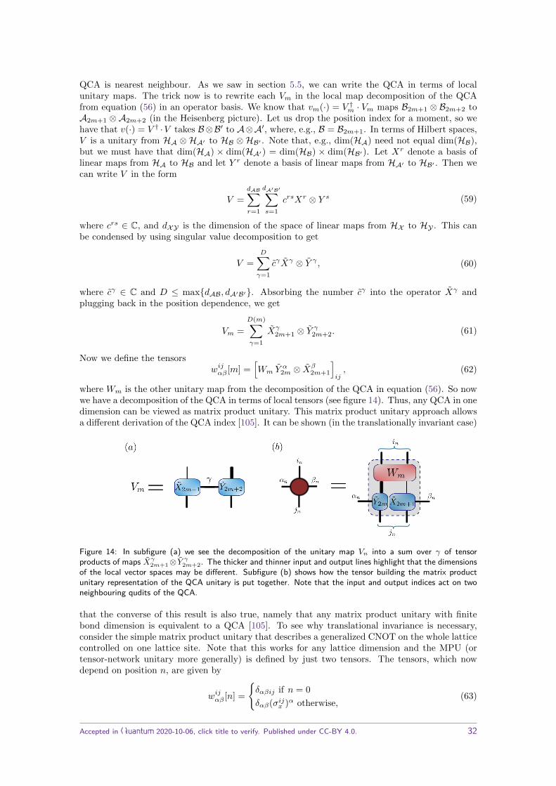
QCA is nearest neighbour. As we saw in section 5.5, we can write the QCA in terms of localunitary maps. The trick now is to rewrite each Vm in the local map decomposition of the QCAfrom equation (56) in an operator basis. We know that vm(·) = V †m · Vm maps B2m+1 ⊗ B2m+2 toA2m+1 ⊗A2m+2 (in the Heisenberg picture). Let us drop the position index for a moment, so wehave that v(·) = V † ·V takes B⊗B′ to A⊗A′, where, e.g., B = B2m+1. In terms of Hilbert spaces,V is a unitary from HA ⊗HA′ to HB ⊗HB′ . Note that, e.g., dim(HA) need not equal dim(HB),but we must have that dim(HA) × dim(HA′) = dim(HB) × dim(HB′). Let Xr denote a basis oflinear maps from HA to HB and let Y r denote a basis of linear maps from HA′ to HB′ . Then wecan write V in the form

V =dAB∑r=1

dA′B′∑s=1

crsXr ⊗ Y s (59)

where crs ∈ C, and dXY is the dimension of the space of linear maps from HX to HY . This canbe condensed by using singular value decomposition to get

V =D∑γ=1

cγXγ ⊗ Y γ , (60)

where cγ ∈ C and D ≤ maxdAB, dA′B′. Absorbing the number cγ into the operator Xγ andplugging back in the position dependence, we get

Vm =D(m)∑γ=1

Xγ2m+1 ⊗ Y

γ2m+2. (61)

Now we define the tensorswijαβ [m] =

[Wm Y

α2m ⊗ X

β2m+1

]ij, (62)

where Wm is the other unitary map from the decomposition of the QCA in equation (56). So nowwe have a decomposition of the QCA in terms of local tensors (see figure 14). Thus, any QCA in onedimension can be viewed as matrix product unitary. This matrix product unitary approach allowsa different derivation of the QCA index [105]. It can be shown (in the translationally invariant case)

Figure 14: In subfigure (a) we see the decomposition of the unitary map Vn into a sum over γ of tensorproducts of maps Xγ

2m+1⊗ Yγ

2m+2. The thicker and thinner input and output lines highlight that the dimensionsof the local vector spaces may be different. Subfigure (b) shows how the tensor building the matrix productunitary representation of the QCA unitary is put together. Note that the input and output indices act on twoneighbouring qudits of the QCA.

that the converse of this result is also true, namely that any matrix product unitary with finitebond dimension is equivalent to a QCA [105]. To see why translational invariance is necessary,consider the simple matrix product unitary that describes a generalized CNOT on the whole latticecontrolled on one lattice site. Note that this works for any lattice dimension and the MPU (ortensor-network unitary more generally) is defined by just two tensors. The tensors, which nowdepend on position n, are given by

wijαβ [n] =δαβij if n = 0δαβ(σijx )α otherwise,

(63)


where all indices take values in 0, 1. Here δαβij is one if all indices are equal and is zero otherwise.Also note that (σijx )α is the Pauli X matrix with matrix indices i, j to the power of α. If we considerthe operator σ0

x, then U†σ0xU =

∏n σ

nx , so U is clearly not locality preserving.

These MPUs can be further classified in the presence of on-site unitary symmetries [108]. Thisworks similarly to the classification of matrix product states in the presence of symmetries [107].The main result of [108] is that one-dimensional matrix product unitaries are completely classifiedby (i) the QCA index and (ii) the cohomology class of the representation of the symmetry groupacting on the bond indices, as conjectured in [109]. The classification considers two matrix productunitaries U0 and U1 to be equivalent if, possibly by adding ancillas transforming under arbitraryrepresentations of the symmetry group, there is a continuous path of matrix product unitaries Utjoining U0 and U1. If we restrict our attention to equivalence under only appending local ancillasthat all transform under the same representation, then the classification can be further refined,though it remains incomplete. Non-unitary symmetries, relevant for, e.g., the tenfold way incondensed matter physics, are discussed in [105], where (i) complex conjugation, (ii) transpositionand (iii) time-reversal symmetric MPUs are classified to some extent. In this case, the classificationof matrix product unitaries that are symmetric under complex conjugation is complete.

Further developments have been made recently relating tensor networks and QCAs. First, theconnection between one-dimensional fermionic QCAs and fermionic matrix product states is nowunderstood [110]. This is trickier than in the qudit case: a very natural definition for fermionicmatrix product states was shown not to capture all fermionic QCAs [110]. In fact, it is theMajorana shift that we saw in equation (50) in section 5.2.3 that provides a counterexample. Tocircumvent this problem, the definition of fermionic matrix product states is extended to includeancillary degrees of freedom at each site. Then a subset of these tensor networks does include allfermionic QCAs. This allows a re-derivation of the fermionic QCA index we saw in section 5.2.3.

Another recent development was that qudit QCAs in any spatial dimension can be viewedas tensor-network unitaries with bond dimension independent of the system size [62]. The onlyrequirement is that the tensors satisfy a property called simplicity, which ensures that the actionof the tensor-network must be locality-preserving. (For most tensor networks, this property seemsdifficult to verify, as it is not a local criterion but rather requires contracting the entire tensornetwork.) A consequence of this equivalence is that the entanglement created by QCAs alwaysobeys an area law. Furthermore, this formalism also extends naturally to the non-unitary case,where the dynamics is a completely positive trace-preserving map. In that case, however, tensornetworks with bond dimension independent of the system size are not always enough to describethe dynamics.

6 QCAs in physics

Aside from being a model for quantum computation, QCAs arise in physics, for example, aseffective models for Floquet dynamics or as proposals for quantum simulators. One of the reasonsthis is natural is because QCAs have an inherent maximum speed of propagation of information.Depending on the setting, this speed can be identified either with the speed of light if we areapproximating a relativistic system with a QCA; or we can identify it with the speed of sound orLieb-Robinson velocity if we are approximating non-relativistic systems. In the following sections,we will look at both of these applications, but first let us look in more detail at the differencesbetween QCA dynamics and continuous-time Hamiltonian evolution.

6.1 QCAs vs Hamiltonian dynamics

We can simulate the dynamics of continuous-time systems on lattices with local Hamiltonians byusing the Suzuki-Trotter decomposition [17, 111, 112]. By ordering the unitary gates in the rightway [57], we get a QCA. A different approach uses Lieb-Robinson bounds [24] to ensure thatwe can approximate continuous-time dynamics with high accuracy using a QCA [113, 114]. Forany such simulation methods to work, it is essential that the continuous-time model has some


approximate locality-preserving property, e.g., it obeys Lieb-Robinson bounds. On the other hand,continuous-time evolution cannot be strictly locality preserving. Let us convince ourselves of thisfact.

Consider qudits on a lattice, evolving via the local time-independent Hamiltonian H. Here,local means that the Hamiltonian is a sum of local terms, i.e., H =

∑X∈X hX , where X are all

d-dimensional hypercubes on the lattice of size at most ld, where l is a positive integer and d is thelattice dimension, and hX is an operator acting non-trivially only on qudits in X. And consider anoperator localized at site ~0 at t = 0, so A ∈ A~0. Now suppose the dynamics is locality preservingin a strict sense. This means that there would be some time T such that, for all t < T , theevolved operator eiHtAe−iHt is strictly contained within some finite region R containing the point~0. So, for any B localized outside of R and any t < T , we must have [B, eiHtAe−iHt] = 0. Taylorexpanding for small t, we get

[B, eiHtAe−iHt] = [B,A] + i[B, [H,A]]t+O(t2) = 0, (64)

where we can use [B,A] = 0 to get

[B, [H,A]] +O(t) = 0. (65)

We can take t to be as small as we wish, so the second term on the second line can be madearbitrarily small. Therefore, the first term [B, [H,A]] must be zero. We can do the same for thehigher order terms, and we see that all the nested commutators must vanish, e.g., [B, [H, [H,A]]] =0. But this means that [B, eiHtAe−iHt] = 0 for all t, which tells us that the operator eiHtAe−iHt

never actually has support outside of the region R for any time t. And this is true for any A ∈ A~0.

Hence, if information is ever going to spread from ~0 to outside R, it does so immediately, thoughwith a very small amplitude in general.

This simple argument shows us why we need to consider discrete time for lattice systems if wewant our dynamics to be strictly locality preserving.

Another interesting question regarding the connection between Hamiltonians and QCAs iswhether there is a natural way to associate a Hamiltonian to a QCA.13 For finite lattices, wealways have a unitary U implementing the dynamics, so we can define H by U = e−iH . Adrawback of this prescription is that it is not unique because we can add multiples of 2π to theeigenvalues of H and still get the same U . Furthermore, this Hamiltonian will generally not bestrictly local14 (i.e., a sum of local operators on the lattice), as can be seen by writing H = i ln(U),defined as a power series:

H = i ln(U) = −i∞∑n=1

(1− U)n

n, (66)

which holds as long as ‖U − 1‖ < 1 [116]. This contains interactions between sites arbitrarily faraway from each other, though the strength of the interaction between sites decays with distance.Interestingly, one can construct QCAs such that all Hamiltonians H satisfying U = e−iH are fullynon-local, meaning that the interaction terms in H between different regions do not decay withdistance [117]. For this to be possible, the unitary must violate ‖U − 1‖ < 1, so that the righthand side of equation (66) does not converge.

A related question for QCAs is whether there is a meaningful notion of a ground state or energyordering. Because the eigenvalues of a unitary are complex phases, there is no natural way to orderthe eigenvalues. This means that there is no clear way to decide which state has the lowest energy.For simulating dynamics via QCAs, this may not be much of a problem, but this is important totake into consideration if we wish to view QCAs as something more fundamental. This is becauseunderstanding low energy and ground state properties of physical systems plays a huge role in, e.g.,condensed matter and high energy physics. But for Hamiltonians there is a natural ground state

13The analogous question of finding a Hamiltonian for continuous-time dynamics obeying a Lieb-Robinson boundhas a positive answer [115].

14Another option for finding a Hamiltonian corresponding to a QCA is to consider i(U −U†), which is self adjointthough generally not a sum of local terms.


and a meaningful notion of an energy gap. At the moment, there appears to be nothing similarfor QCAs.

There is one final setting where QCAs arise naturally: as approximations to or toy models forperiodically driven quantum systems, also known as Floquet quantum systems [118]. Suppose wehave a lattice system and a time-dependent Hamiltonian H(t) that is periodic with period T , i.e.,for all t,

H(t+ T ) = H(t). (67)The Schrodinger equation is

i∂

∂t|ψ(t)〉 = H(t)|ψ(t)〉. (68)

This has solutions [118]

|Ψα(t)〉 = e−iεαt|Φα(t)〉where |Φα(t+ T )〉 = |Φα(t)〉.

(69)

Here, εα are found by solving (H(t)− i∂/∂t)|Φα(t)〉 = εα|Φα(t)〉. These are called quasi-energies,and they are real and unique up to adding integer multiples of 2π/T . If we restrict our attentionto times t = nT , where n ∈ Z, then we have a discrete-time system evolving via Un, where U is aunitary operator, given by

U = T exp(−i∫ T

0dtH(t)

), (70)

where T is the time-ordering operator. Typically, U will not be locality preserving, but even inthe time-dependent case, Lieb-Robinson bounds are enough to guarantee that we can approximatethe dynamics well with a QCA [113, 114]. This allows us to use QCAs as toy models for Floquetsystems and to use QCA techniques to understand some of their properties, as we will see in thefollowing section.

6.2 Dynamical topological phases in Floquet systems

In general, topological phases of matter are phases that do not fit well into the classification ofphases in terms of symmetry breaking [119]. Instead, they are classified by topological properties ofthe system. A key example is the integer quantum Hall effect, where the topological classificationarises from Chern numbers in the TKNN formula for the Hall conductivity [120]. The quantizedHall conductivity can be observed when such a system (which consists of non-interacting particles)is at temperatures low compared to the gap, and so the system is close to its ground state. Thenone observes the existence of chiral edge modes: in the two-dimensional bulk of the material thesystem is actually an insulator, but along the boundary these chiral edge modes allow the materialto conduct. A requirement for this phenomenon to occur is that there is some disorder in thesystem, which leads to localization in the material.

The integer quantum Hall effect involves the low temperature physics of static systems. But wemay also ask whether similar phenomena can occur in dynamical systems. To answer this question,dynamical topological phases have been introduced and classified in Floquet systems [121–124] fornon-interacting particles. These are called anomalous Floquet-Anderson insulators, and one againsees the presence of propagating edge modes on a two-dimensional material. It became clear laterin [25, 26] that this phenomenon can persist even in the presence of interactions. Here we will lookat the models given in [25], which display this behaviour, admitting information propagation onlyalong the boundary.

The paradigmatic example is quite intuitive and works as follows. Take a two-dimensionallattice Γ, where each site has d dimensional qudits. Suppose the system evolves by a simple QCA,which is a depth-four quantum circuit, where each unitary in the circuit is simply a swap, asdepicted in figure 15 (a). Let ~e1 and ~e2 be lattice basis vectors and denote the swap between sites~n and ~n+ ~ei as S~n,~n+~ei . Define the sublattice

Γeven = (n,m) ∈ Γ|n+m is even. (71)


We consider evolution viaU = U[+~e2]U[−~e1]U[−~e2]U[+~e1], (72)

where

U[±~ei] =∏

~n∈Γeven

S~n,~n±~ei . (73)

This is easiest to understand by looking at figure 15 (a). If Γ is the infinite plane or a torus,

Figure 15: Subfigure (a) shows the Floquet dynamics on the infinite plane. The green swaps are applied first,orange are second, purple third and blue swaps are applied last. By following the path of a qudit, we see thatthe dynamics after all four swaps is the identity. In subfigure (b) however, a boundary has been introduced, andwe can see that some of the qudits at the boundary have nontrivial dynamics.

then it is clear that U is actually just the identity: a qudit gets moved around a plaquette backto where it started. On the other hand, if we introduce a boundary, then qudits in the bulk stillstay put after one timestep, but qudits at the edge propagate. See figure 15 (b). Notice that inthis case we have a one-dimensional QCA at the boundary: a shift of d-dimensional qudits eachtimestep. By layering two of these two-dimensional systems on top of each other, where one hasd1-dimensional qudits at each site undergoing the evolution given above, and the other layer hasd2-dimensional qudits at each site undergoing the inverse evolution, we get a trivial bulk theorybut a one-dimensional QCA on the boundary with index d1/d2. The central idea of [25] is thatthis index classifies the chiral propagation on the boundary and hence the topological phase. Theexamples here with qudits are then representatives for each different phase, as we can get a QCAwith any boundary index with the right choice of d1 and d2.

Of course, any phase classification is physically meaningless without some sort of stabilityagainst perturbations. We already know that the index is stable with respect to local perturbations(see section 5.2), so this classification should be stable with respect to local defects at the boundary,but what about bulk perturbations? This is where assuming localization comes in. Just as was thecase for the integer quantum Hall effect, we need to demand that the systems under considerationhave some form of localization to ensure that we get well-defined phases. In this case, becausewe are dealing with interacting systems, we make the requirement that the system is many-bodylocalized. Let us take a quick detour to introduce many-body localization in Floquet systems.

We take as our definition for a many-body localized Floquet unitary U that (for an infinitelattice system) there exists a localization length ξ, such that

U =∏~n

V~n, (74)

where [V~n, V~m] = 0 and V~n is supported on a region N(~n) centred on ~n of radius ξ.15 (Actually, weneed only require that V~n is approximately supported on N(~n), allowing some exponential decay

15Note that, if we relax the commutation criterion, then any unitary arising from finite-time Hamiltonian evolutioncan be approximated in this form as a finite-depth local unitary circuit.


outside.) As a very simple example, consider qubits with

W =∏~n

exp (−iπJ~nZ~n) , (75)

where J~n are real numbers. This is just a product of on-site unitaries and so is clearly many-bodylocalized in this sense.

We will use this many-body localization property to define the phases in a way that is stableagainst bulk perturbations. To do this, we look at two unitary operators that act on the infinitesystem Γinf and the system with boundary Γfin. First, for dynamics on the unbounded system Γinf ,we have a decomposition of the dynamics into local commuting unitaries because we are assumingmany-body localization. Then, for the system with boundary, we may define a unitary operatorfrom a product of these local unitaries restricted to Γfin to be

Ulc =∏~n

N(~n)⊂Γfin

U~n, (76)

where the product only includes terms that are localized on the system Γ. Importantly, thisis not the actual dynamics of the system. Instead, that is given by considering which physicalHamiltonian terms act on the system

Udyn = T exp(−i∫ T

0dtHfin(t)

), (77)

where Hfin(t) is the Hamiltonian consisting of terms contained in Γfin. The exact details of Hfin(t)do not matter, but Udyn itself does. For example, in the simple four-step swap dynamics weconsidered in equation (72), Udyn just involves swaps on the lattice between subsets of vertices. Inthat case, where there is a boundary, some swaps do not occur because there is nothing to swapwith, as in figure 15 (b).

Now we define Y = (Ulc)†Udyn. Because of the many-body localization property, this can onlybe a non trivial unitary close to the boundary, as the local unitaries in (Ulc)† cancel the bulkdynamics in Udyn. We classify the phases according to the QCA index of Y as a one-dimensionalboundary QCA. Let us see how this works for the swap example.

Suppose we augment the swap evolution defined in equation (73) with local commuting unitariesW =

∏~nW~n, so that now the dynamics are given by

U = WU[+~e2]U[−~e1]U[−~e2]U[+~e1]. (78)

On an infinite lattice or discrete torus, we know that U[+~e2]U[−~e1]U[−~e2]U[+~e1] = 1. Therefore,

Ulc =∏

~n∈Γfin

W~n. (79)

As we saw earlier, on the system with boundary U[+~e2]U[−~e1]U[−~e2]U[+~e1] is just a shift along the

boundary, which we will denote by SB , so that Udyn = WSB . But then Y = (Ulc)†Udyn is simplythe shift of qudits along the boundary SB . This has index d.

There is an important point regarding this phase classification that we have glossed over. Inreality, a QCA will only be an approximation to the actual dynamics. However, by choosing theneighbourhood size of the QCA to be at least as big as the Lieb-Robinson cone after one periodof the dynamics T , this will be a very good approximation [113]. One might speculate that theclassification via the index theory may not work simply because the index may not stop changingas we consider better and better approximations to the true dynamics (which will have largerand larger neighbourhoods), and it is conceivable that the index could converge to an irrationalnumber. It may be that this concern is unwarranted, especially if one considers, e.g., the caseof qubits, where the index must always be an integer power of two. Then the allowed index


values are not dense in R, so the index cannot converge to anything other than a power of two(or zero). Nevertheless, it would be a worthwhile pursuit to extend the index theory to almostlocality-preserving unitaries to back up this intuition.

A proposal for actually measuring the index characterizing information flow along the boundaryof a two-dimensional Floquet system has been made [125].

6.3 Understanding phases of matter

As mentioned before, a central problem in condensed matter physics is understanding quantumphases of matter. Essentially, two systems described by local or quasi-local Hamiltonians H0 andH1 are in the same phase if there is a continuous path of Hamiltonians Hs with s ∈ [0, 1] joiningthem. However, there are further requirements that the path must preserve. Typically, H0 andH1 will be gapped Hamiltonians, so the path Hs must also be gapped. In some further cases, H0and H1 will have some symmetry, such as time-reversal or chiral symmetry, which must also bepreserved along the path. These latter cases are symmetry-protected phases.

Classifying such phases of matter has seen a lot of success in one dimension, with all Hamilto-nians being classified. In two dimensions, there is no full classification, but there are examples ofHamiltonians displaying non-trivial topological order, such as Levin-Wen models [126]. In higherdimensions, there are more exotic examples still, suggesting the possible phases are even morerich. One such example in three dimensions, where QCAs play a role, is a specific case of theWalker-Wang model [127, 128]. This model is only topologically interesting at boundaries, andwith boundary conditions chosen to include all possible boundary terms still supported in the sys-tem, it is believed that topological order appears. The 3-fermion Walker-Wang model consists of athree-dimensional lattice with two qubits on the links (analogous to lattice gauge theories, wherephysical degrees of freedom live on the links between sites, rather than at the sites themselves).Much like the toric code, an example of a lattice gauge theory, the Hamiltonian is a sum of com-muting local Pauli operators. Furthermore, with periodic boundary conditions, the ground stateis unique [27].

One concept that plays a role here is triviality of QCAs, introduced in section 3.1. Recall thata QCA u is called trivial if it is a product of local finite-depth circuits and shifts possibly by addinglocal ancillas. In other words, if u is trivial, then u⊗ 1 can be decomposed in terms of shifts anda local finite-depth circuit.

In [27] a QCA uWW is explicitly constructed as a disentangler (defined below) of the groundstate of this Walker-Wang model. The consequences of this are interesting. If this QCA is trivial,then there exists a two-dimensional commuting projector Hamiltonian that realizes the topologicalorder of the Walker-Wang model. This works by considering the Walker-Wang model on a latticethat is infinite in the x and y directions but semi-infinite in the z direction (with z coordinatein (−∞, 0]). If the QCA is trivial, then we could use it to disentangle the ground state in thetwo-dimensional boundary plane at z = 0 from the bulk. Then we could construct a commutingprojector model for this two-dimensional plane, which has topological order.

However, realizing the topological order of the Walker-Wang model with a two-dimensionalcommuting projector Hamiltonian is believed to be impossible [27]. This in turn suggests thatuWW cannot be trivial. Further evidence is given in [27] for this: uWW is a Clifford QCA, but isnontrivial as a Clifford QCA, meaning it cannot be written as a product of shifts and local-finitedepth Clifford circuits. Also if uWW is trivial, then there must exist a fermionic QCA in twodimensions that is nontrivial. So there is a guarantee that some nontrivial QCA exists.

Let us look at some of the methods used to arrive at these results. A useful concept introducedin [27] is that of locally flippable separators. These are a generalization of the Clifford elements X~nand Z~n for qudits, introduced in section 3.2. To understand this, first we need to define separators,which generalize the qudit Z~n operators.

Definition 6.3.1. A separator for a lattice system consists of some label set L and unitary oper-ators Za with a ∈ L that satisfy the following properties.


1. All Za have even parity (only necessary for fermionic degrees of freedom).

2. [Za,Zb] = 0 for all a, b ∈ L.

3. There is a l ∈ Z, which is small compared to the dimensions of the lattice, such that everyZa is contained in a hypercube with length of side l.

4. For each a, there is an integer Da with ZDaa = 1 and Da ≥ 2.

5. For every possible choice of map a→ ω(a), where ω(a) is a Dath root of one, there is a singlestate satisfying Za|ψ〉 = ω(a)|ψ〉.

The states |ψ〉 in the definition are analogous to qudit stabilizer states. In fact, a separator iscalled trivial if the labels can be chosen such that lattice sites ~n and labels a ∈ L are in one-to-onecorrespondence with Z~n = Za (for fermion modes, this is replaced by 2a†~na~n − 1 = Za).

Then a local flipper is analogous to the X~n operators for qudits.

Definition 6.3.2. A local flipper Xa for a separator Za is a set of unitary operators with the samelabel set L that satisfies the properties below.

1. Xa has odd parity if Za is a fermionic operator.

2. [Xa,Zb] = 0 for all a, b ∈ L with a 6= b. Otherwise, ZbXa = e2πi/DaXaZb

3. There is a l ∈ Z, which is small compared to the dimensions of the lattice, such that everyXa is contained in a hypercube with length of side l.

Note that there is no assumption about the commutation or anticommutation relations betweenXa and Xb for a 6= b. A locally flippable separator is a separator that has a local flipper.

A central result in [27] is the following theorem for which we only state the qudit case. Thecase with fermionic degrees of freedom involves some additional complexity because it is necessaryto add ancillary degrees of freedom.

Theorem 6.3.3. Any locally flippable separator can be mapped to a trivial separator by a QCA,which is said to disentangle the locally flippable separator.

The role this plays for the Walker-Wang model is that the ground state can be viewed asa locally flippable separator, and hence this theorem guarantees that the ground state can bedisentangled via a QCA, namely uWW .

These disentangling methods play a role also in [76], where they are used to construct nontrivialClifford QCA in three dimensions with qudits with any prime dimension. The examples again arisefrom topological models, in this case via coupled toric codes that have toplogical order on a surface.

QCAs play another role in classifying topological phases. In [129], the symmetries of sub-systems of a two-dimensional system are described by QCAs. In this case, this allows a deeperunderstanding of the connection between symmetry-protected topological order and measurement-based quantum computation.

In [130], an exactly solvable 4+1 dimensional model with a Z2 symmetry is introduced which isoutside the classification by cohomology. The Walker-Wang model again plays a role here, and wealso see the effective realization of the symmetry on a subsystem (in this case a 3 + 1 dimensionalboundary) by a QCA. Interestingly, this QCA is inequivalent to a finite-depth quantum circuitand is in fact nontrivial.

6.4 QCAs and particles

In this and the following sections we will construct QCAs that have a clear interpretation in termsof particles. To do this, it is natural to first look at the single-particle analogues of QCAs, which


are called discrete-time quantum walks. These consist of a single quantum particle evolving on alattice unitarily, with the restriction that the particle can hop at most by a bounded distance eachtimestep.16 This is the single-particle version of locality preservation. These discrete-time quantumwalks have many nice properties: with the right choice of unitary, we recover relativistic dynamicsin the continuum limit, e.g., [37]; the symmetry-protected topological phases of these models canbe classified [131–134]; and they also have more direct applications in quantum computing [135].

With this in mind, it is interesting to consider the possibility of constructing QCAs that aresimply many-particle versions of these quantum walks. As a consequence, in the non-interactingsetting much of the analysis that applies for quantum walks (e.g., the classification of topologicalphases) should also apply to these QCAs. On the other hand, we can also add interactions andarrive at entirely new physics. Before considering how to upgrade quantum walks to QCAs, let uslook at a particularly important example of a quantum walk.

Consider a quantum particle on a discrete line with coordinates n ∈ Z and an extra two-dimensional degree of freedom with basis states |l〉 and |r〉. Then an orthonormal basis of thewhole Hilbert space is simply given by |n〉|l〉 and |n〉|r〉 where n ∈ Z. We define the unitaryσx = |l〉〈r|+ |r〉〈l|, and then we can consider the following unitary implementing the evolution:

U = e−imσxa(|r〉〈r|S + |l〉〈l|S†

), (80)

where m ∈ R, a is the lattice spacing, and S is a shift for a single particle, i.e., S|n〉 = |n+ 1〉 forall n. Notice that the dynamics is translationally invariant. In the continuum limit, m will be themass. The term on the right in brackets is a conditional shift: if the particle is in the r state, itmoves one step to the right, and if it is in the l state, it moves one step to the left. If we switch tomomentum space, we have

|p〉 =√a∑n∈Z

eipna|n〉, (81)

where p ∈ (−π/a, π/a] is the lattice momentum and 〈p|q〉 = 2πδ(p − q). In this basis, the shiftis just a phase S|p〉 = e−ipa|p〉. Then, defining σz = |r〉〈r| − |l〉〈l|, we can rewrite the conditionalshift as

|r〉〈r|S + |l〉〈l|S† = e−iPσza, (82)

where P =∫ dp

2πp|p〉〈p| is the lattice momentum operator. This allows us to write the evolutionoperator as

U = e−imσxae−iPσza. (83)

Acting on smooth states (those with bounded momenta |p| ≤ Λ π/a), we can look at manytimesteps N = t/a, to get

UN =(e−imσxae−iPσza

)N= 1 +−i(Pσz +mσx)t+O(Λ2a2)= e−i(Pσz+mσx)t +O(Λ2a2).

(84)

As long as we choose our cutoff Λ to grow sufficiently slowly as a→ 0, we get a sensible continuumlimit, with the last line above corresponding to evolution via the one-dimensional Dirac equationwith Hamiltonian H = Pσz +mσx. A lot of interesting work has been done using this simple yetpowerful quantum walk [38, 136, 137]. This includes studying, e.g., how mass mixes chiralities andZitterbewegung [138].

We can also construct quantum walks in higher dimensional spaces that give rise to relativisticparticles in the continuum limit [37], which is in some sense generic [139]. For example, to discretizethe Weyl equation, we take a cubic lattice with coordinates ~n ∈ Z3 and let the particle have a two

16In some contexts, e.g., quantum search algorithms, discrete-time quantum walks are defined without the restric-tion on the hopping range.


dimensional extra degree of freedom with orthonormal basis states |↑z〉 and |↓z〉, which correspondto spin in the continuum limit.17 The evolution operator is

U = TxTyTz

= e−iPxσxae−iPyσyae−iPzσza,(85)

where Tb = | ↑b〉〈↑b |Sb + | ↓b〉〈↓b |S†b is a conditional shift along the b axis depending on the spinin the b direction.18 We can take the continuum limit of this quantum walk just as we did for theone-dimensional case, which is done rigorously (an explicit proof of convergence for regular initialconditions is given) for this quantum walk and more in [140]. In the continuum limit, the dynamics

is described by the Weyl equation with Hamiltonian H = ~P .~σ [37]. It is straightforward to extendthis to, e.g., the massive Dirac equation in three dimensional space.

There are at least two natural ways to upgrade single-particle quantum walk dynamics toQCAs. One way goes via quantum lattice gases, and the other is by second quantization. It isworth highlighting that we can discretize many physical models with quantum walks, e.g., Dirac orWeyl particles in curved spacetime [141–144] or in external gauge fields [39, 145, 146] or both [147],and so these models can also be upgraded to QCAs. As an aside, it is also possible to constructthe Feynman propagator in some cases for quantum walks [148].

6.4.1 Lattice gases

The study of quantum lattice gases dates back to the early days of QCAs [42, 149–152], and anice discussion can be found in [153]. The dynamics, which is generally taken to be translationallyinvariant, consists of two steps: a step where particles on the lattice propagate without interaction,and an interaction (or scattering) step between particles on the same site. So the idea is that eachlattice site has up to d particles. For each particle, there is a k-dimensional qudit, with algebrasBj~n ∼= Mk, which describes the states of the jth particles at that site. As Bj~n corresponds to ak-dimensional quantum system, each particle has k−1 possible internal states, with the remainingstate corresponding to the empty state |q~n,j〉, which represents the absence of the particle. The

algebra for each site is then A~n = ⊗jBj~n.

To define the dynamics, we choose d lattice vectors ~ei, and the propagation step simply shiftsthe jth particle by ~ej , meaning

σ : Bj~n → Bj~n+~ej . (86)

The interaction step is a product of on-site unitaries, which are the same at each site:

v~n : A~n → A~n. (87)

The dynamics comprises the propagation step followed by the scattering step, u = vσ. Quantumlattice gas automata are usually defined with a quiescent state. For finite systems this has theform

|q〉 =⊗~n∈Γ

k⊗j=1|q~n,j〉, (88)

where Γ denotes the spatial lattice (this state also makes sense for infinite systems, where it isdefined by its expectation values). This carries the interpretation of the completely empty state,i.e., the state with no particles at all present.

Let us consider an example in one dimension that corresponds to a lattice gas version of thesingle-particle evolution in equation (83). (Because that single-particle evolution is translationallyinvariant, the dynamics makes sense on a finite system with periodic boundary conditions, as longas the length of the system is large compared to the maximum distance the particle can hop overa single timestep, but the lattice gas approach also works for infinite systems.) Suppose that each

17This is in contrast to the one-dimensional case, where |l〉 and |r〉 correspond to chirality in the continuum limit.18| ↑b〉 and | ↓b〉 are the +1 and −1 eigenvectors of the bth Pauli matrix respectively.


lattice site has two qubits labelled by l and r. So the on-site algebra is An = Bln ⊗ Brn. Let thequiescent state be the zero state of all qubits

|q〉 =⊗n∈Γ

k⊗j=1|0〉, (89)

where Γ = 0, ..., N − 1. And if any qubit is in the |1〉 state, then there is a particle present. Forexample if the l qubit at site n is in the one state, there is an l type particle at site n. We choosethe propagation step to simply shift the l qubits left and the r qubits right, so

σ :Bln → Bln+1Brn → Brn−1.

(90)

The interaction term at site n is then implemented by the unitary (dropping the n subscripts)

V = |00〉〈00|+ cos(ma)[|01〉〈01|+ |10〉〈10|

]− i sin(ma)

[|01〉〈10|+ |01〉〈10|

]+ eiφ|11〉〈11|, (91)

where |ab〉 denotes a state with a ∈ 0, 1 l particles present and b ∈ 0, 1 r particles present.Here we see that V preserves the empty state, as |00〉 is taken to |00〉, while the left and righthanded particles are mixed to some degree by the mass term. We have some freedom left (afterdemanding that the single-particle sector evolves as the original quantum walk), which involveschoosing the phase that is applied when both particle types are present eiφ. We can use this tomodel an on-site interaction between the particles.

A general recipe for upgrading quantum walks to QCAs in a way similar to quantum latticegases also appeared in [19, 33, 154]. It is also interesting to look at this from a different perspective:we may ask when are QCAs equivalent to quantum lattice gases [68], in other words, when do theyallow a particle interpretation in the way we have described here? It has been shown that one canconstruct QCAs that cannot be written as quantum lattice gases despite propagating information[153]. Even taking products of quantum lattice gas automorphisms does not generate all QCAs[153]. Finally, it is worth mentioning that a general proposal for discretizing fermions interactingwith gauge fields via quantum lattice gases was given in [155, 156].

6.4.2 Fermions

Next we consider the second option, which is second quantization.19 We will only look at fermionicsecond quantization here, but it is also possible for bosons. In fact, the lattice gases of theprevious section could be considered as hardcore bosons, which are bosons with an on-site repulsiveinteraction that is so strong that only one boson of that type may be present at each site. Let usgo through how fermionic second quantization works. To every state |α〉 of an orthonormal basisof our original single-particle system, we associate a fermion creation operator ψ†α, such that

ψα, ψ†β = δαβ

ψα, ψβ = 0.(92)

In the many-particle Hilbert space there is an empty state |0〉, which is annihilated by all theannihilation operators, i.e., ψα|0〉 = 0 for all α. Next we may define a linear map Q from single-particle states to creation operators, which we can also define for adjoints. Given a single-particlestate |v〉 =

∑α cα|α〉, Q is defined by

Q(|v〉)

=∑α

cαψ†α

Q(〈v|)

=∑α

c∗αψα.(93)

19Incidentally, second quantization is not a particularly good name. We are just constructing a many-particlequantum system that acts like many copies of a single-particle one; we are not making the theory more quantum!


This also extends to operators on the single-particle space in a natural way. Consider the single-particle Hamiltonian h =

∑E E|E〉〈E|, then we have

Q(h)

=∑E

Eψ†EψE , (94)

where ψE = Q(〈E|). Now, we can upgrade our quantum walk operator in equation (83) to a QCAevolution operator. First, denote a complete set of annihilation operators corresponding to thesingle-particle states |n〉|l〉 and |n〉|r〉 as ψnl and ψnr. For compactness, we can write this as atwo-component operator ψn = (ψnr, ψnl)T . Analogously to the single-particle case, we can switchto momentum space, and we have the two-component momentum space annihilation operator

ψp =√a∑n

e−ipnaψn. (95)

Then the Dirac QCA in one dimension has evolution operator given by

W = exp(−ima

∫ dp2π ψ

†pσxψp

)exp

(−ia

∫ dp2π pψ

†pσzψp

). (96)

It is straightforward to check that this gives the correct dynamics, e.g., W τψ†n|0〉 evolves exactlyas a one-particle state should over τ timesteps. The second term above is a conditional fermionicshift: it shifts ψnl to the left and ψnr to the right. This is clearly locality preserving, as is the firstterm above: by switching to position space we see that

exp(−ima

∫ dp2π ψ

†pσxψp

)=∏n

exp(−imaψ†nσxψn

), (97)

which is a product of on-site unitaries. Therefore, W itself is also locality preserving.

Of course, the main reason for using second quantization is to look at interacting systems,which works via adding another unitary step to the dynamics, e.g.,

V = exp(−iλ

∑n

ψ†nlψnlψ†nrψnr

), (98)

which gives a phase if there are two particles at the same site, analogously to an energy penalty,e.g., from Coulomb repulsion of electrons. Then the overall dynamics is given by U = VW , and thisQCA is referred to as a Thirring QCA [157]. This is essentially a second-quantized version of theinteracting quantum walks considered in [158, 159]. For other studies of interacting two-particlequantum walks, see [160, 161].

6.5 Quantum field theory

A good reason to discretize quantum field theories with QCAs is that they are already algorithmsfor simulating the dynamics of QFTs on a quantum computer, which retain some of the niceproperties of QFTs like strict causality, i.e., locality preservation. However, any QCA discretizationbreaks Lorentz symmetry, something that also occurs for lattice quantum field theory. Nevertheless,some attempts have been made to introduce a discrete version of Lorentz symmetry for QCAs[162]. One approach is to consider a change of observer as a change of representation of thedynamics (without explicit reference to spacetime), which can be done in such a way as to reproducethe familiar Lorentz group in the low momentum regime for Dirac and Weyl QCAs [163]. Theemergence of a modification of special relativity, doubly special relativity (where there is a frame-invariant length as well as speed) was also studied for QCAs in one dimension [164].

It is interesting that strongly interacting QFTs are often defined to be the continuum limit oflattice quantum field theories (i.e., lattice models with local Hamiltonians) [165]. So QCAs mayoffer an alternative definition of some QFTs too. An early work on the connection between QCAs


and field theory is given for example in [166], though this differs at least superficially from ournotion of QCAs in the following way: to update the system to timestep τ + 1, one needs to knowthe state at times τ and τ − 1.

Recently, several quantum algorithms have been proposed that efficiently simulate some quantumfield theories (φ4 theory [167] and the Gross-Niveau model [168]). These algorithms did not useQCAs to simulate the dynamics but rather Suzuki-Trotter decompositions of the evolution oper-ator (e−iHt, where H is the Hamiltonian of a suitable lattice QFT). However, an important pointto highlight here is that the difficult part of these proposals was not simulating the dynamics butrather the initial state preparation [167, 168]. Nevertheless, it is interesting to consider QCAs asnatural discrete models, which provide alternative options for quantum simulations. One advant-age of a QCA approach could be their simplicity: for example, to simulate the dynamics of Weylfermions via a QCA, we need only implement swaps on the lattice [61, 169]. Interactions are thenprovided, as in equation (98), by on-site unitaries.

A nice example of a QCA was introduced in [170] that discretizes a fermionic QFT called themassive Thirring model (though the work actually pre-dates QCAs and so does not use the nameQCA). After taking a (not so rigorous) continuum limit of the QCA, the dynamics is given by theHamiltonian

H =∫ dp

2π ψ†p(pσz +mσx)ψp + 2g

∫dxψ†l (x)ψl (x)ψ†r(x)ψr(x), (99)

where g is a constant. The rightmost term is the interaction term, so setting g = 0 would simplygive us free Dirac fermions in one dimension. A QCA that discretizes this was already given in theprevious section: the QCA is a lattice system with fermionic creation and annihilation operatorswith extra index l and r, and the evolution operator is given by

U = exp(−iλ

∑n

ψ†nlψnlψ†nrψnr

)exp

(−ima

∫ dp2π ψ

†pσxψp

)exp

(−ia

∫ dp2π pψ

†pσzψp

). (100)

Recall that ψpl and ψpr are the Fourier transforms of ψnl and ψnr respectively, and ψp = (ψpr, ψpl)T .Here, we can naively see that the continuum limit dynamics should correspond to the Hamiltonianin equation (99). How one shows this is given in detail in [170], though the evolution operator forthe QCA is slightly different in that case, but the basic idea is the same. See also [157].

A crucial point to bear in mind is that the discrete analogue of the physical ground state is notthe state |0〉 annihilated by all the annihilation operators ψnα. This is because the vacuum in QFTis a highly entangled state [67], and the QCA must reproduce this entanglement in the continuumlimit. Even in non-interacting QFTs, there is vacuum entanglement, so we cannot simulate theQFT ground state via the naive QCA vacuum state |0〉, which has no entanglement. For theone-dimensional massless Dirac QCA (equation (96) with m = 0), convergence of the QCA to themassless Dirac field was shown in [57], a consequence of which was that there is a choice of QCAvacuum that converges to the quantum field vacuum.

There has been a lot of work on discretizing and simulating non-interacting fermionic fieldsby QCAs [61, 169, 171–177], which consider Dirac and Weyl QCAs in higher dimensional spaces.Furthermore, the one-dimensional Dirac QCA model was actually recently re-derived in a QFTcontext [178]. Of course, the more interesting cases are QCAs that discretize interacting quantumfield theories, as in the example given in equation (100). Another example of an interacting fermionQCA that discretizes an interacting quantum field theory, in this case quantum electrodynamicsin one spatial dimension, was given in [179]. Furthermore, for interacting bosonic quantum fieldtheories, such as φ4 theory and non-abelian gauge theories, the discrete-time path integral fromlattice QFT is actually exactly equivalent to a QCA [22].

Another interesting discrete model of a quantum field theory is the so-called QCA theory oflight [180]. This is not dissimilar to a discretized version of the neutrino theory of light [181]and constructs a QCA approximating quantum electromagnetism (without matter) from two WeylQCAs in three dimensional space. At a very superficial level, the main idea is to use that the


vector of Pauli matrices ~σ transforms like

exp(− i2~v.~σ

)σi exp

(i

2~v.~σ)

=∑j

[exp

(−i~v. ~J

)]ijσj , (101)

where Ji form a representation of the generators of the Lie algebra of SO(3) given by [Ji]jk =−i∑j,k εijk, where i, j, k all take values in 1, 2, 3. Then, roughly speaking, the dynamics causes

a bilinear fermion field Mi(~p) = ψ~p σiΨ~p to evolve as

Mi(p, t) =∑j

[e−i2~p. ~Jt]ijψ~p σjΨ~p =∑j

[e−i2~p. ~Jt]ijMj(p, t), (102)

where ψ~p and Ψ~p are two different two-component fermion fields in momentum space. This isequivalent to

− i∂t ~M(~p, t) = ~p× ~M(~p, t). (103)

We then define the electric and magnetic field operators in terms of Mi

Ei(~p, t) = M†i (~p, t) +Mi(~p, t)

Bi(~p, t) = i(M†i (~p, t)−Mi(~p, t)).(104)

If we also introduce the constraint that ~p. ~M(~p, t) = 0, then we recover Maxwell’s equations for Eiand Bi. Of course, there are many details that have been swept under the rug here, which aredealt with in [180]. For example, one also has to ensure that the correct commutation relationsfor Ei and Bi are recovered. Another point about the model is that it is not clear how to extendit to an interacting model via coupling to matter because the electric ~E(~x) and magnetic fields~B(~x) are the fundamental quantities in the QCA, as opposed to the electromagnetic four-vectorpotential Aµ(~x). Due to phenomena like the Aharanov-Bohm effect, one would expect that any

direct coupling of the ~E(~x) and ~B(~x) fields to matter would have to be non-local.

7 Outlook and open problems

We have looked at many interesting aspects of quantum cellular automata, including their usein quantum computation, QCA structure theorems, and their role in physics, e.g., as models ofFloquet topological phases; in understanding phases of matter; or as quantum field theories. Itis remarkable how versatile the QCA model has been, and how many varied applications it hashad. It is interesting then to speculate on the future of QCAs. For example, currently there areseveral different efforts to discretize QFTs in terms of QCAs, and it is not inconceivable that thestandard model of particle physics could have a QCA discretization. An argument supportingthis possibility is that many QFTs already have a QCA representation, from Dirac fermions tonon-abelian gauge theories. However, one roadblock to be overcome is fermion doubling, which tothis day causes issues in classical and quantum simulations of lattice QFT.

Another fascinating topic is the connection between topological phases of matter and QCAs(e.g., as disentanglers). It is fascinating to speculate on what can be gained by combining thisapproach with the tensor-network picture of QCAs, as the latter has proved to be a very usefulrepresentation for classifying phases of matter. Progress in this regard has been fast: in the firstversion of this review, one of the open problems asked if one can generalize the correspondencebetween matrix product unitaries and QCAs to higher dimensional systems. This was just solvedin [62]. Because tensor networks help to understand the role of symmetries in phase classifications,it seems that there is a lot of potential to study phases further using QCAs.

With all this in mind, there are currently many fascinating open problems related to QCAs.Below we list some concrete problems as well as some possible ideas to tackle them.

1. In terms of quantum computation, one interesting question that arose before was whetherthere is a meaningful notion of QCA error correction? If many different single or two-qubit


gates are needed, as opposed to a small set of global operations, then it is not clear why QCAquantum computation would be sensible instead of simply focussing on the circuit model orthe measurement-based model. In other words, is there a comprehensive theory of quantumcomputation using QCAs including all necessary aspects?

2. Fully classifying QCAs in dimensions greater than two remains open. The classificationin terms of the index and topology of the control space (section 5.3) was quite elegantand complete in two dimensions, so it is natural to wonder what extra invariants there arebeyond two dimensions. And how does the classification change depending on how we defineequivalence of two QCAs (e.g., whether we allow appending ancillas at each site or not)?

3. What can be said about essentially local QCAs, i.e., those with only approximately localitypreserving dynamics, as opposed to the strict locality preservation we considered here? If weallow tails with a suitable notion of decay, what results for strictly local QCAs survive? Thishas relevance for, e.g., the use of QCAs as toy models for understanding Floquet topologicalphases in section 6.2.

4. What can be said about irreversible QCAs, which had only received little attention in, e.g.,[18, 52]? At the moment, there are only constructive definitions. For example, it makes senseto give examples of irreversible QCAs by taking a finite-depth circuit of local completely pos-itive trace-preserving maps. But is there any reasonable axiomatization that seems physicallymotivated and which also allows useful structure theorems? Even for probabilistic classicalcellular automata, this is not at all straightforward [182]. However, progress has been madevery recently in [62], where the connection to tensor networks allowed some investigation of avery general definition of irreversible QCAs. It seems likely that the methods considered therewill allow further insight into irreversible QCAs, and maybe even some form of classification.

5. What can QCAs tell us about the structure of quasi-local algebras on infinite systems?Boundary algebras (defined similarly to the support algebras of section 5.2.1 [76]) can beused as a tool to define the one-dimensional index, but in higher dimensions, where the al-gebraic structure becomes very interesting, boundary algebras of QCAs give rise to nontrivialdecompositions of quasi-local algebras [76]. There may be deep connections between QCAsand the structure of infinite-lattice qudit or fermion algebras that remain to be found.

6. When does it make sense to talk about ground states for QCAs? A related question iswhether there is any systematic way (other than exact diagonalization for finite systems) tofind invariant states for QCAs, perhaps by getting some local constraints on the state. Onemight then in some cases try to define a ground state for a QCA by finding an invariant purestate that has low entanglement. For some ideas in this direction, see [52].

7. What more can be said about QCAs with symmetries? For example, when is there asymmetry-protected topological classification of QCAs in one dimension (with symmetriesas in the tenfold way, which are a combination of time-reversal, chiral and particle-hole sym-metry [183])? Progress in this direction has already been made for one-dimensional QCAs viathe matrix product unitary approach as discussed in section 5.6, as these approaches allowsome classification of some unitary and antiunitary symmetries for one-dimensional QCAs.

8. How can we take continuum limits of interesting QCAs? So far all models with continuumlimits are integrable (solvable in some sense). It is not clear how to go beyond this. In latticeQFT, continuum limits are typically signalled by a second order phase transition. Is thereany analogue of this for QCAs? In some cases, the path integral formulation of lattice QFTis actually equivalent to a QCA [22], which might provide some insight. Another idea wouldbe to use the framework for general continuum limits from [184]. Also interesting in thisregard are the coherent families of [103], or the more abstract generalization of QCAs [185].


Acknowledgements

The author is grateful to Pablo Arrighi, Cedric Beny, Alessandro Bisio, Tobias Geib, JeongwanHaah, Norm Margolus, Tobias Osborne, Asif Shakeel and Reinhard Werner for useful suggestionsand feedback. The author was supported by the Australian Research Council Centres of Excellencefor Engineered Quantum Systems (EQUS, CE170100009).

A Infinite systems and quasi-local algebras

In this section, we will look at the basics of C*-algebras, particularly those describing infinite spinlattices. Some good references are [59, 60, 186]. One of the key features of C*-algebras is thepossible existence of inequivalent representations, which is the reason we deal with the abstractalgebra itself rather than any particular representation in terms of operators on a Hilbert space.This is related to the existence of superselection sectors, see [187].

Let us start with the definition of a C*-algebra.

Definition A.0.1. A C*-algebra A is a complex algebra with a norm ‖ · ‖ in which it is completeas a vector space (making it a Banach space) and with an anti-linear map, A → A∗, which is aninvolution, with the following properties:

1. (AB)∗ = B∗A∗

2. ‖AB‖ ≤ ‖A‖‖B‖

3. ‖A∗‖ = ‖A‖

4. ‖A∗A‖ = ‖A‖2.

We will also assume that our C*-algebras have an identity. It is useful to keep in mind thatany closed set of bounded operators on a Hilbert space is a C*-algebra, where the * operation isjust the adjoint. And a special case of this is Mn(C), the set of n× n complex matrices. Since itis finite dimensional, this example misses out on the subtleties associated to infinite dimensions.

We will focus on the C*-algebra description of quantum lattice systems. We start with thelattice Zd which has a finite dimensional quantum system associated to each point. Then, to eachlattice site there is an associated finite dimensional C*-algebra that is equivalent to Mn(C) forsome n. Next we associate a finite dimensional C*-algebra AΛ to any finite region Λ of the lattice,such that AΛ is isomorphic to a tensor product of the algebras associated to each site in Λ. TheC*-algebra of a subset Λ′ of Λ is identified with the elements in AΛ that act like the identity onΛ\Λ′. So far this is similar to the usual quantum theory with a finite number of subsystems, andit would be exactly equivalent if the lattice were finite.

For any finite Λ, the norm on elements of AΛ is equivalent to the operator norm on thecorresponding operators on the finite dimensional system associated to Λ.

When we consider the whole lattice Zd, the C*-algebra is a vector space that includes allelements that are non-trivial only on a finite subset of Zd. And to get the full C*-algebra, wecomplete this vector space, by including Cauchy sequences of elements that converge in the norm.So the total C*-algebra contains local elements that are non-trivial on a finite subset of Zd andquasi local elements, which can be approximated arbitrarily well by sums of local elements.

Let us define isomorphisms of C*-algebras (*-isomorphisms). First, a morphism (or *-morphism)π between two C*-algebras A and B is a linear map preserving the algebraic structure:

1. π(A)π(B) = π(AB) ∀A ∈ A, ∀B ∈ B,

2. π(A∗) = π(A)∗ ∀A ∈ A.


An isomorphism is an invertible morphism. An example of an isomorphism on our quantum latticesystem in the case of qubits is the conjugation of each site’s algebra by Xn, i.e., A → XnAXn

for any A ∈ An. It follows that the elements of the algebra associated to larger finite regions areconjugated by tensor products of Xs. Intuitively, this looks like applying the map A → XAX forany A ∈ A, where X = ⊗m∈ZXm. Notice that X is not in the C*-algebra itself.

As mentioned above, a closed set of bounded operators on a Hilbert space is an example of aC*-algebra. Thanks to the following theorem by Gel’fand and Naimark, it is the only example.

Theorem A.0.2. Any C*-algebra is isomorphic to a C*-algebra of operators on a Hilbert space.

But the catch is that this Hilbert space may not be separable.

A positive element of a C*-algebra, written as A ≥ 0, is self adjoint with a real positivespectrum. Saying an element A is positive is equivalent to saying that there exists a B ∈ A suchthat A = B∗B. This allows us to define states on a C*-algebra.

Definition A.0.3. A state on a C*-algebra ω is a linear functional that is positive, meaningω(A) ≥ 0 if A ≥ 0 and normalised, meaning ω(1) = 1.

For the C*-algebraMn(C) corresponding to an n-dimensional qudit, we can identify states withelements ofMn(C), since finite dimensional vector spaces are isomorphic to their dual spaces. Werecover the familiar density matrix formalism, with ρ(A) = tr[ρA], where ρ is a positive semi-definite matrix in Mn(C), and tr[·] is the trace.

For our quasi-local algebra, we do not need to think in terms of abstract functionals. It isequivalent to associate a density operator to each finite subregion of the lattice. This worksprovided the family of states satisfies a natural consistency condition: given ρΛ′ and ρΛ are densityoperators associated to the finite regions Λ′ and Λ, with Λ′ ⊆ Λ, then

ρΛ′ = trΛ\Λ′ [ρΛ]. (105)

A representation of a C*-algebra A is a morphism π from A to a set of bounded operatorson a Hilbert space. A faithful representation is one where π is an isomorphism. If we have arepresentation π of a C*-algebra acting on the Hilbert space H, then, for any φ ∈ H, the closureof the subspace spanned by π(A)φ with A ∈ A, Hφ, is left invariant by the action of all π(A). Sowe may as well focus on representations with Hφ = H. These are called cyclic representations andφ is called a cyclic vector. Note that if we normalise φ then it defines a state on A via

ω(A) = (φ, π(A)φ). (106)

The following theorem provides the GNS construction, which allows us to construct a representationusing any state on A.

Theorem A.0.4. Given a state ω on A, there exists a cyclic representation of A with a cyclicvector φ, such that

ω(A) = (φ, π(A)φ). (107)

Furthermore, this representation is unique up to unitary equivalence, meaning that, if there aretwo cyclic representations of A on H1 and H2 such that

ω(A) = (φ1, π1(A)φ1) = (φ2, π2(A)φ2), (108)

then there is a unique unitary map U from H1 to H2 such that φ2 = Uφ1 and π2(A) = Uπ1(A)U−1

for all A ∈ A.

The proof entails using the state to define an inner product on the C*-algebra via20

∀ A,B ∈ A (A,B) ≡ ω(A∗B). (109)

20If ω(A) = 0 for some A ≥ 0, then we have to work with the quotient of A by all B ∈ A with ω(B∗B) = 0.


This inner product gives us a Hilbert space with vectors A ∈ A. In particular, 1 ∈ A is thoughtof as φ, since

ω(1A1) = ω(A) ≡ (φ, πω(A)φ). (110)

Then the representation of the elements in A as operators on this Hilbert space is simply

π(B)φA ≡ BA, (111)

where A is thought of as a vector here. Although mathematically we think of A ∈ A as vectors ina Hilbert space, it is also useful to think of these vectors as arising from the action of A on thestate ω ≡ φω.

A good example of a representation involves the spin lattice C*-algebra. Take ω to be the statewith all spins pointing up along the z-direction, meaning

ωΛ ≡⊗i∈Λ

(1 00 0

)(112)

for all finite regions Λ. A basis for Hω is given by vectors we can think of as⊗i∈Λ

| ↓〉i⊗

i∈Zd\Λ

| ↑〉i, (113)

for all finite regions Λ. So the representation is spanned by all states with only a finite number ofspins pointing down.

Let us now look at automorphisms, which are just isomorphisms from the C*-algebra to itself.The following interesting result is a consequence of theorem A.0.4.

Corollary A.0.5. Given an automorphism α of a C*-algebra A, and a state ω with cyclic repres-entation (πω,Hω, φω), then α can be implemented by a unitary on Hω such that

π(α(A)) = Uπ(A)U−1 (114)

andUφω = φω (115)

if and only ifω(A) = ω(α(A)), (116)

and U is uniquely determined.

An example of an automorphism that is not implementable in a representation as a unitary isthe application of Pauli Xs everywhere in the spin lattice representation given above in equation(113). This follows since flipping all the spins from up to down is not an operation that is allowedin the Hilbert space.

B QCAs with fermions

For fermionic QCAs, instead of having qudits at each site we have some number of fermionic modes.(We could also consider hybrid QCAs with both qudits and some fermion modes at each site.) Thesimplest way to describe fermion systems is via their creation and annihilation operators (creationoperators are just adjoints of annihilation operators). A nice discussion of finite fermionic algebrasis given in [101]. We denote the annihilation operators by aα, where α is a label in some set. Forexample, if we have a single fermion mode on each lattice site, we would take α to be a vector inZd. For simplicity, let us choose the index to run over Z. The creation and annihilation operatorsobey the anticommutation relations:

aα, aβ = 0

aα, a†β = δαβ .(117)


Furthermore, we can construct our Hilbert space by starting with a state |0〉 that satisfies

aα|0〉 = 0 (118)

for all α. This state has the interpretation as being empty. The empty state also makes sense forinfinite lattices of fermions, where it is defined to be a positive normalized functional ω0 satisfying

ω0[a†αaα] = 0 (119)

for all α. The operator a†αaα counts the number of fermions in the mode labelled by α and haseigenvalues 0 and 1. The state a†α|0〉 has the interpretation as having a single fermion present.Furthermore, it follows from the anticommutation relations that a†2α = 0, which means that we canhave at most one fermion in each mode.

We can also define Majorana fermion operators, which are sometimes more convenient to workwith. These are defined to be

c2α = a†α + aα

c2α+1 = i(a†α − aα).(120)

These are self-adjoint and satisfy the anticommutation relations

cn, cm = 2δnm. (121)

Most of the details of the quasi-local algebra approach to defining infinite systems of fermionsare similar to the qudit case. We assign fermionic algebras to regions of the lattice. The maindifference with the qudit case is that creation and annihilation operators from different regions ormodes anticommute. See [60] for a detailed discussion.

Another way to think about fermion systems is via graded algebras. In a graded algebra wehave some basis of operators with the following property: each element is either even or odd. Thisalso extends easily to hybrid systems of qudits and fermions. For example, the fermion algebra wehave already seen is a graded algebra, with, e.g., 1 and a†αaα being even elements whereas aα areodd. A linear combination of an even and an odd operator is neither even nor odd.

Let us take a step back and start with the graded Hilbert space H (really we mean Z2 graded).We decompose H = He ⊕Ho, where Ho is the odd subspace and He is the even subspace. Thesewill correspond to the subspaces with odd and even fermion number respectively. One can also usethe notation Cp|q, where p and q are the dimensions of the even and odd subspaces respectively.We define even operators to be those that preserve evenness or oddness, e.g., they map even statesto even states. Odd operators are then those that map the even subspace to the odd subspace andvice versa.

This leads naturally to the graded commutator. We can write this as [·, ·, and it is defined tobe bilinear and satisfy

[A,B = A,B if A and B are odd[A,B = [A,B] if at least one of A and B are even.

(122)

So, for example, if A and B are odd and C is even, we have

[A,B + C = A,B+ [A,C]. (123)

We can introduce a graded tensor product too. The tensor product of two graded Hilbertspaces is also a graded Hilbert space. A tensor product of vectors that are both even or both oddis even. A tensor product of vectors that have opposite grading is odd. So we denote the gradedtensor product of H1 and H2 by H1 ⊗g H2. Then we have

(H1 ⊗g H2)e = (He1 ⊗He2)⊕ (Ho1 ⊗Ho2)(H1 ⊗g H2)o = (He1 ⊗Ho2)⊕ (Ho1 ⊗He2) .

(124)

The graded tensor product of graded algebras is similar: a graded tensor product of even operatorsis an even operator, for example. After taking the graded tensor product of two graded algebras Aand B, even elements of, e.g., A and all elements of B commute. Furthermore, we say two algebrasA and B graded commute if [A,B = 0 for all A ∈ A and all B ∈ B.


References[1] J. von Neumann. Theory of Self-Reproducing Automata. University of Illinois Press, Cham-

paign, Illinois, 1966.[2] A. W. Burks, editor. Essays on Cellular Automata. University of Illinois Press, Champaign,

Illinois, 1970.[3] M. Delorme. An introduction to cellular automata. In J. Mazoyer M. Delorme, editor,

Cellular Automata: a Parallel Model, pages 5–49. Springer, Netherlands, 1999. DOI:https://doi.org/10.1007/978-94-015-9153-9˙1.

[4] E. R. Berlekamp, J. H. Conway, and R. K. Guy. Winning Ways for Your Mathematical Plays,volume 2. Academic Press, London, 1982. DOI: https://doi.org/10.1201/9780429487323.

[5] S. Wolfram. Statistical mechanics of cellular automata. Rev. Mod. Phys., 55:601–644, 1983.DOI: https://doi.org/10.1103/RevModPhys.55.601.

[6] M. Cook. Universality in elementary cellular automata. Complex Systems, 15:1 – 40, 2004.[7] T. Neary and D. Woods. P-completeness of cellular automaton rule 110. In

M. Bugliesi, B. Preneel, V. Sassone, and I. Wegener, editors, Automata, Languagesand Programming, pages 132–143, Berlin, Heidelberg, 2006. Springer. DOI: ht-tps://doi.org/10.1007/11786986˙13.

[8] B. Chopard. Cellular Automata Modeling of Physical Systems, pages 407–433. Springer, NewYork, 2012. DOI: https://doi.org/10.1007/978-1-4939-8700-9˙57.

[9] S. Succi. The Lattice Boltzmann Equation For Fluid Dynamics and Beyond. ClarendonPress, Oxford, 2001.

[10] D. A. Wolf-Gladrow. Lattice-Gas Cellular Automata and Lattice Boltzmann Models: anIntroduction, volume 1725 of Lecture Notes in Mathematics. Springer, Berlin, 2000. DOI:https://doi.org/10.1007/b72010.

[11] P. Arrighi and J. Grattage. The quantum game of life. Physics World, 25(06):23, 2012. DOI:https://doi.org/10.1088/2058-7058/25/06/37.

[12] R. P. Feynman. Simulating physics with computers. International Journal of TheoreticalPhysics, 21:467–488, 1982. DOI: https://doi.org/10.1007/bf02650179.

[13] A. Trabesinger. Quantum simulation. Nature Physics, 8:263, 2012. DOI: ht-tps://doi.org/10.1038/nphys2258.

[14] N. Margolus. Quantum computation. Annals of the New York Academy of Sciences, 480(1):487–497, 1986. DOI: https://doi.org/10.1111/j.1749-6632.1986.tb12451.x.

[15] S. Lloyd. A potentially realizable quantum computer. Science, 261(5128):1569–1571, 1993.DOI: https://doi.org/10.1126/science.261.5128.1569.

[16] J. Watrous. On one-dimensional quantum cellular automata. Proceedings of the 36th An-nual IEEE Symposium on Foundations of Computer Science, pages 528–537, 1995. DOI:https://doi.org/10.1109/sfcs.1995.492583.

[17] M. A. Nielsen and I. L. Chuang. Quantum Computation and Quantum Information. Cam-bridge University Press, Cambridge, 2000. DOI: https://doi.org/10.1017/cbo9780511976667.

[18] G. K. Brennen and J. E. Williams. Entanglement dynamics in one-dimensionalquantum cellular automata. Phys. Rev. A, 68:042311, 2003. DOI: ht-tps://doi.org/10.1103/PhysRevA.68.042311.

[19] B. Schumacher and R. F. Werner. Reversible Quantum Cellular Automata. arXiv:0405174,2004.

[20] P. Arrighi, V. Nesme, and R. F. Werner. Unitarity plus causality implies localiz-ability. Journal of Computer and System Sciences, 77(2):372–378, 2011. DOI: ht-tps://doi.org/10.1016/j.jcss.2010.05.004.

[21] D. Tong. The unquantum quantum. Scientific American, 307:46–49, 2012. DOI:https://doi.org/10.1038/scientificamerican1212-46.

[22] T. Farrelly and J. Streich. Discretizing quantum field theories for quantum simulation.arXiv:2002.02643, 2020.

[23] K. Wilson. The renormalization group and critical phenomena. In Nobel Lectures, Physics1981-1990. World Scientific, 1993.


https://doi.org/https://doi.org/10.1007/978-94-015-9153-9_1


https://doi.org/https://doi.org/10.1201/9780429487323

https://doi.org/https://doi.org/10.1103/RevModPhys.55.601

https://doi.org/https://doi.org/10.1007/11786986_13



https://doi.org/https://doi.org/10.1007/b72010

https://doi.org/https://doi.org/10.1007/b72010

https://doi.org/https://doi.org/10.1088/2058-7058/25/06/37


https://doi.org/https://doi.org/10.1007/bf02650179

https://doi.org/https://doi.org/10.1038/nphys2258

https://doi.org/https://doi.org/10.1038/nphys2258

https://doi.org/https://doi.org/10.1111/j.1749-6632.1986.tb12451.x

https://doi.org/https://doi.org/10.1126/science.261.5128.1569

https://doi.org/https://doi.org/10.1109/sfcs.1995.492583

https://doi.org/https://doi.org/10.1109/sfcs.1995.492583

https://doi.org/https://doi.org/10.1017/cbo9780511976667

https://doi.org/https://doi.org/10.1103/PhysRevA.68.042311


https://doi.org/https://doi.org/10.1016/j.jcss.2010.05.004


https://doi.org/https://doi.org/10.1038/scientificamerican1212-46

https://doi.org/https://doi.org/10.1038/scientificamerican1212-46

http://arxiv.org/abs/2002.02643

[24] E. H. Lieb and D. W. Robinson. The finite group velocity of quantum spin sys-tems. Communications in Mathematical Physics, 28(3):251–257, 1972. DOI: ht-tps://doi.org/10.1007/bf01645779.

[25] H. C. Po, L. Fidkowski, T. Morimoto, A. C. Potter, and A. Vishwanath. Chiral Flo-quet phases of many-body localized bosons. Phys. Rev. X, 6:041070, 2016. DOI: ht-tps://doi.org/10.1103/PhysRevX.6.041070.

[26] L. Fidkowski, H. C. Po, A. C. Potter, and A. Vishwanath. Interacting invariants forFloquet phases of fermions in two dimensions. Phys. Rev. B, 99:085115, 2019. DOI: ht-tps://doi.org/10.1103/PhysRevB.99.085115.

[27] J. Haah, L. Fidkowski, and M. B. Hastings. Nontrivial Quantum Cellular Automata inHigher Dimensions. arXiv:1812.01625, 2018.

[28] B. Aoun and M. Tarifi. Introduction to Quantum Cellular Automata. arXiv:quant-ph/0401123, 2004.

[29] J. Horowitz. An introduction to quantum cellular automata, 2008.http://web.mit.edu/joshuah/www/projects/qca.pdf.

[30] K. Wiesner. Quantum cellular automata. In Encyclopedia of Complexity and Systems Science,pages 7154–7164. Springer, 2009. DOI: https://doi.org/10.1007/978-3-642-27737-5˙426-4.

[31] W. van Dam. Quantum cellular automata. Master’s thesis, University of Nijmegen, 1996.[32] C. A. Perez Delgado. Quantum Cellular Automata: Theory and Applications. PhD thesis,

University of Waterloo, 2007.[33] H. Vogts. Discrete time quantum lattice systems. PhD thesis, Technische Universitat Braun-

schweig, 2009.[34] P. Arrighi. Quantum cellular automata. Habilitation thesis, Universite de Grenoble, 2009.[35] J. Gutschow. Quantum information processing with Clifford quantum cellular automata. PhD

thesis, Leibniz Universitat Hannover, 2012.[36] P. Arrighi. An overview of quantum cellular automata. Nat Comput, 18:885–899, 2019. DOI:

https://doi.org/10.1007/s11047-019-09762-6.[37] I. Bialynicki-Birula. Weyl, Dirac, and Maxwell equations on a lattice as unitary cellular auto-

mata. Phys. Rev. D, 49:6920–6927, 1994. DOI: https://doi.org/10.1103/PhysRevD.49.6920.[38] F. W. Strauch. Relativistic quantum walks. Phys. Rev. A, 73:054302, 2006. DOI: ht-

tps://doi.org/10.1103/PhysRevA.73.054302.[39] C. Cedzich, T. Rybar, A. H. Werner, A. Alberti, M. Genske, and R. F. Werner. Propaga-

tion of quantum walks in electric fields. Phys. Rev. Lett., 111:160601, 2013. DOI: ht-tps://doi.org/10.1103/PhysRevLett.111.160601.

[40] G. Grossing and A. Zeilinger. Quantum cellular automata. Complex Systems, 2(2):197–208,1988.

[41] D. A. Meyer. On the absence of homogeneous scalar unitary cellular automata. PhysicsLetters A, 223(5):337–340, 1996. DOI: https://doi.org/10.1016/s0375-9601(96)00745-1.

[42] D. A. Meyer. From quantum cellular automata to quantum lattice gases. Journal of StatisticalPhysics, 85:551–574, 1996. DOI: https://doi.org/10.1007/bf02199356.

[43] C. S. Lent, P. D. Tougaw, W. Porod, and G. H. Bernstein. Quantum cellular automata.Nanotechnology, 4(1):49, 1993. DOI: https://doi.org/10.1088/0957-4484/4/1/004.

[44] P. D. Tougaw and C. S. Lent. Logical devices implemented using quantum cellular automata.Journal of Applied Physics, 75(3):1818–1825, 1994. DOI: https://doi.org/10.1063/1.356375.

[45] G. Toth and C. S. Lent. Quantum computing with quantum-dot cellular automata. Phys.Rev. A, 63:052315, 2001. DOI: https://doi.org/10.1103/PhysRevA.63.052315.

[46] C. A. Perez-Delgado and D. Cheung. Models of Quantum Cellular Automata. arXiv:quant-ph/0508164, 2005.

[47] D. Nagaj and P. Wocjan. Hamiltonian quantum cellular automata in one dimension. Phys.Rev. A, 78:032311, 2008. DOI: https://doi.org/10.1103/PhysRevA.78.032311.

[48] K. G. H. Vollbrecht and J. I. Cirac. Quantum simulators, continuous-time automata,and translationally invariant systems. Phys. Rev. Lett., 100:010501, 2008. DOI: ht-tps://doi.org/10.1103/PhysRevLett.100.010501.

[49] G. ’t Hooft. The Cellular Automaton Interpretation of Quantum Mechanics. Springer, NewYork, 2016. DOI: https://www.doi.org/10.1007/978-3-319-41285-6.

[50] S. Wolfram. A new kind of science. (Self-published) Wolfram Media Inc., 2002.




https://doi.org/https://doi.org/10.1103/PhysRevX.6.041070


https://doi.org/https://doi.org/10.1103/PhysRevB.99.085115



http://arxiv.org/abs/quant-ph/0401123


http://web.mit.edu/joshuah/www/projects/qca.pdf

https://doi.org/https://doi.org/10.1007/978-3-642-27737-5_426-4

https://doi.org/https://doi.org/10.1007/s11047-019-09762-6


https://doi.org/https://doi.org/10.1103/PhysRevD.49.6920



https://doi.org/https://doi.org/10.1103/PhysRevLett.111.160601


https://doi.org/https://doi.org/10.1016/s0375-9601(96)00745-1



https://doi.org/https://doi.org/10.1063/1.356375







https://doi.org/https://www.doi.org/10.1007/978-3-319-41285-6

[51] S. Aaronson. Limits on Efficient Computation in the Physical World. PhD thesis, Universityof California, Berkeley, 2004.

[52] S. Richter and R. F. Werner. Ergodicity of quantum cellular automata. Journal of StatisticalPhysics, 82(3):963–998, 1996. DOI: https://doi.org/10.1007/BF02179798.

[53] C. A. Perez-Delgado and D. Cheung. Local unitary quantum cellular automata. Phys. Rev.A, 76:032320, 2007. DOI: https://doi.org/10.1103/PhysRevA.76.032320.

[54] N. Margolus. Parallel quantum computation. In W. H. Zurek, editor, Complexity, Entropy,and the Physics of Information, page 273, Redwood City, CA, 1991. Addison Wesley.

[55] P. Arrighi and V. Nesme. Quantization of cellular automata. JAC 2008, pages 204–215,2008.

[56] P. Arrighi, V. Nesme, and R. F. Werner. Bounds on the speedup in quantum signaling. Phys.Rev. A, 95:012331, 2017. DOI: https://doi.org/10.1103/PhysRevA.95.012331.

[57] T. C. Farrelly. Insights from Quantum Information into Fundamental Physics. PhD thesis,University of Cambridge, 2015. arXiv:1708.08897.

[58] O. Kruger and R. F. Werner. Gaussian quantum cellular automata. In N. Cerf, G. Leuchs, andE. S. Polzik, editors, Quantum Information with Continuous Variables of Atoms and Light.Imperial College Press, London, 2007. DOI: https://doi.org/10.1142/9781860948169˙0005.

[59] P. Naaijkens. Quantum spin systems on infinite lattices. arXiv:1311.2717, 2013.[60] O. Bratteli and D. Robinson. Operator Algebras and Quantum Statistical Mechanics, volumes

1 and 2. Springer, Berlin, 1997. DOI: https://doi.org/10.1007/978-3-662-03444-6.[61] T. C. Farrelly and A. J. Short. Causal fermions in discrete space-time. Phys. Rev. A, 89:

012302, 2014. DOI: https://doi.org/10.1103/PhysRevA.89.012302.[62] L. Piroli and J. I. Cirac. Quantum cellular automata, tensor networks, and area laws.

arXiv:2007.15371, 2020.[63] M. Freedman and M.B. Hastings. Classification of quantum cellular automata. Communica-

tions in Mathematical Physics, 376:1171–1222, 2020. DOI: https://doi.org/10.1007/s00220-020-03735-y.

[64] P. Perinotti and L. Poggiali. Scalar fermionic cellular automata on finite Cayley graphs.arXiv:1807.08695, 2018.

[65] P. Arrighi, V. Nesme, and R. F. Werner. One-dimensional quantum cellular automataover finite, unbounded configurations. In Language and Automata Theory and Applica-tions, volume 5196 of Lecture Notes in Computer Science, pages 64–75. Springer, 2008. DOI:https://doi.org/10.1007/978-3-540-88282-4˙8.

[66] A. Shakeel. Quantum Cellular Automata: Schrodinger and Heisenberg Pictures.arXiv:1807.01192v1, 2018.

[67] S. J. Summers and R. Werner. The vacuum violates Bell’s inequalities. Physics Letters A,110(5):257 – 259, 1985. DOI: http://doi.org/10.1016/0375-9601(85)90093-3.

[68] A. Shakeel and P. J. Love. When is a quantum cellular automaton (QCA) a quantumlattice gas automaton (QLGA)? Journal of Mathematical Physics, 54(9):092203, 2013. DOI:https://doi.org/10.1063/1.4821640.

[69] D. M. Schlingemann, H. Vogts, and R. F. Werner. On the structure of Clifford quantumcellular automata. Journal of Mathematical Physics, 49(11):112104, 2008. DOI: ht-tps://doi.org/10.1063/1.3005565.

[70] J. Gutschow, S. Uphoff, R. F. Werner, and Z. Zimboras. Time asymptotics and entanglementgeneration of Clifford quantum cellular automata. Journal of Mathematical Physics, 51(1):015203, 2010. DOI: http://doi.org/10.1063/1.3278513.

[71] J. Gutschow. Entanglement generation of Clifford quantum cellular automata. AppliedPhysics B, 98(4):623–633, 2010. DOI: https://doi.org/10.1007/s00340-009-3840-1.

[72] J. Gutschow, V. Nesme, and R. F. Werner. The fractal structure of cellular automata onabelian groups. Discrete Mathematics & Theoretical Computer Science, DMTCS Proceedingsvol. AL, Automata 2010 - 16th Intl. Workshop on CA and DCS, 2010.

[73] J. Haah. Algebraic methods for quantum codes on lattices. Revista Colombiana deMatematicas, 50:299 – 349, 2016. DOI: https://doi.org/10.15446/recolma.v50n2.62214.

[74] S. Gopalakrishnan and B. Zakirov. Facilitated quantum cellular automata as simple modelswith non-thermal eigenstates and dynamics. Quantum Science and Technology, 3(4):044004,2018. DOI: https://doi.org/10.1088/2058-9565/aad759.


https://doi.org/https://doi.org/10.1007/BF02179798






https://doi.org/https://doi.org/10.1007/978-3-662-03444-6



https://doi.org/https://doi.org/10.1007/s00220-020-03735-y

https://doi.org/https://doi.org/10.1007/s00220-020-03735-y





https://doi.org/http://doi.org/10.1016/0375-9601(85)90093-3





https://doi.org/http://doi.org/10.1063/1.3278513


https://doi.org/https://doi.org/10.15446/recolma.v50n2.62214

https://doi.org/https://doi.org/10.1088/2058-9565/aad759

[75] H. Kim, T. N. Ikeda, and D. A. Huse. Testing whether all eigenstates obey theeigenstate thermalization hypothesis. Phys. Rev. E, 90:052105, 2014. DOI: ht-tps://doi.org/10.1103/PhysRevE.90.052105.

[76] J. Haah. Clifford quantum cellular automata: Trivial group in 2d and Witt group in 3d.arXiv:1907.02075, 2019.

[77] D. Gross, V. Nesme, H. Vogts, and R.F. Werner. Index theory of one dimensional quantumwalks and cellular automata. Communications in Mathematical Physics, 310:419–454, 2012.DOI: https://doi.org/10.1007/s00220-012-1423-1.

[78] A. Molina and J. Watrous. Revisiting the simulation of quantum Turing ma-chines by quantum circuits. Proc. R. Soc. A., 475:20180767, 2019. DOI: ht-tps://doi.org/10.1098/rspa.2018.0767.

[79] R. Raussendorf. Quantum cellular automaton for universal quantum computation. Phys.Rev. A, 72:022301, 2005. DOI: https://doi.org/10.1103/PhysRevA.72.022301.

[80] D. J. Shepherd, T. Franz, and R. F. Werner. Universally programmablequantum cellular automaton. Phys. Rev. Lett., 97:020502, 2006. DOI: ht-tps://doi.org/10.1103/PhysRevLett.97.020502.

[81] K. G. H. Vollbrecht and J. I. Cirac. Reversible universal quantum computationwithin translation-invariant systems. Phys. Rev. A, 73:012324, 2006. DOI: ht-tps://doi.org/10.1103/PhysRevA.73.012324.

[82] P. Arrighi, R. Fargetton, and Z. Wang. Intrinsically universal one-dimensional quantumcellular automata in two flavours. Fundamenta Informaticae, 91:197–230, 2009. DOI:https://doi.org/10.3233/FI-2009-0041.

[83] P. Arrighi and J. Grattage. A simple n-dimensional intrinsically universal quantum cellularautomaton. In A. Dediu, H. Fernau, and C. Martın-Vide, editors, Language and AutomataTheory and Applications, pages 70–81, Berlin, Heidelberg, 2010. Springer Berlin Heidelberg.DOI: https://doi.org/10.1007/978-3-642-13089-2˙6.

[84] P. Arrighi and J. Grattage. Intrinsically universal n-dimensional quantum cellular auto-mata. Journal of Computer and System Sciences, 78(6):1883 – 1898, 2012. DOI: ht-tps://doi.org/10.1016/j.jcss.2011.12.008.

[85] P. Arrighi and J. Grattage. Partitioned quantum cellular automata are intrinsically universal.Natural Computing, 11(1):13–22, 2012. DOI: https://doi.org/10.1007/s11047-011-9277-6.

[86] S. Bravyi and A. Kitaev. Fermionic quantum computation. Annals of Physics, 298(1):210 –226, 2002. DOI: https://doi.org/10.1006/aphy.2002.6254.

[87] M. Steudtner and S. Wehner. Fermion-to-qubit mappings with varying resource require-ments for quantum simulation. New Journal of Physics, 20(6):063010, 2018. DOI:https://doi.org/10.1088/1367-2630/aac54f.

[88] S. C. Benjamin. Schemes for parallel quantum computation without local control of qubits.Phys. Rev. A, 61:020301, 2000. DOI: https://doi.org/10.1103/PhysRevA.61.020301.

[89] R. Raussendorf. Quantum computation via translation-invariant operations on a chain ofqubits. Phys. Rev. A, 72:052301, 2005. DOI: https://doi.org/10.1103/PhysRevA.72.052301.

[90] J. A. Jones. Quantum computing with NMR. Progress in Nuclear Magnetic ResonanceSpectroscopy, 59(2):91 – 120, 2011. DOI: https://doi.org/10.1016/j.pnmrs.2010.11.001.

[91] S. C. Benjamin. Quantum computing without local control of qubit-qubit interactions. Phys.Rev. Lett., 88:017904, 2001. DOI: https://doi.org/10.1103/PhysRevLett.88.017904.

[92] S. C. Benjamin and S. Bose. Quantum computing in arrays coupled by “always-on” interac-tions. Phys. Rev. A, 70:032314, 2004. DOI: https://doi.org/10.1103/PhysRevA.70.032314.

[93] J. Twamley. Quantum-cellular-automata quantum computing with endohedral fullerenes.Phys. Rev. A, 67:052318, 2003. DOI: https://doi.org/10.1103/PhysRevA.67.052318.

[94] S. C. Benjamin, A. Ardavan, G. A. D. Briggs, D. A. Britz, D. Gunlycke, J. Jefferson,M. A. G. Jones, D. F. Leigh, B. W. Lovett, A. N. Khlobystov, S. A. Lyon, J. J. L. Mor-ton, K. Porfyrakis, M. R. Sambrook, and A. M. Tyryshkin. Towards a fullerene-basedquantum computer. Journal of Physics: Condensed Matter, 18(21):S867, 2006. DOI:https://doi.org/10.1088/0953-8984/18/21/S12.

[95] T. M. Wintermantel, Y. Wang, G. Lochead, S. Shevate, G. K. Brennen, and S. Whitlock.Unitary and nonunitary quantum cellular automata with Rydberg arrays. Phys. Rev. Lett.,124:070503, 2020. DOI: https://doi.org/10.1103/PhysRevLett.124.070503.


https://doi.org/https://doi.org/10.1103/PhysRevE.90.052105

https://doi.org/https://doi.org/10.1103/PhysRevE.90.052105



https://doi.org/https://doi.org/10.1098/rspa.2018.0767

https://doi.org/https://doi.org/10.1098/rspa.2018.0767






https://doi.org/https://doi.org/10.3233/FI-2009-0041

https://doi.org/https://doi.org/10.3233/FI-2009-0041





https://doi.org/https://doi.org/10.1006/aphy.2002.6254

https://doi.org/https://doi.org/10.1088/1367-2630/aac54f

https://doi.org/https://doi.org/10.1088/1367-2630/aac54f



https://doi.org/https://doi.org/10.1016/j.pnmrs.2010.11.001




https://doi.org/https://doi.org/10.1088/0953-8984/18/21/S12

https://doi.org/https://doi.org/10.1088/0953-8984/18/21/S12


[96] P. Arrighi and S. Martiel. Quantum causal graph dynamics. Phys. Rev. D, 96:024026, 2017.DOI: https://doi.org/10.1103/PhysRevD.96.024026.

[97] A. Kitaev. Anyons in an exactly solved model and beyond. Annals of Physics, 321(1):2 –111, 2006. DOI: https://doi.org/10.1016/j.aop.2005.10.005.

[98] P. Zanardi. Stabilizing quantum information. Phys. Rev. A, 63:012301, 2000. DOI: ht-tps://doi.org/10.1103/PhysRevA.63.012301.

[99] V. Jones and V. S. Sunder. Introduction to Subfactors. London Mathemat-ical Society Lecture Note Series. Cambridge University Press, 1997. DOI: ht-tps://doi.org/10.1017/CBO9780511566219.

[100] P. Jordan and E. Wigner. Uber das Paulische Aquivalenzverbot. Z. Physik, 47:631–651,1928. DOI: https://doi.org/10.1007/BF01331938.

[101] M.A. Nielsen. The fermionic canonical commutation relations and the Jordan-Wigner trans-form, 2005. http://michaelnielsen.org/blog/archive/notes/fermions and jordan wigner.pdf.

[102] J. Baez. The Ten-Fold Way (Part 3), blog post at “The n-Category Cafe”, 2014. ht-tps://golem.ph.utexas.edu/category/2014/08/the tenfold way part 3.html.

[103] M. Freedman, J. Haah, and M. B. Hastings. The group structure of quantum cellular auto-mata. arXiv:1910.07998, 2019.

[104] T. Toffoli and N. H. Margolus. Invertible cellular automata: A review. Physica D: NonlinearPhenomena, 45(1):229 – 253, 1990. DOI: https://doi.org/10.1016/0167-2789(90)90185-R.

[105] J. I. Cirac, D. Perez-Garcia, N. Schuch, and F. Verstraete. Matrix product unitaries: struc-ture, symmetries, and topological invariants. Journal of Statistical Mechanics: Theory andExperiment, 2017(8):083105, 2017. DOI: https://doi.org/10.1088/1742-5468/aa7e55.

[106] M. B. Sahinoglu, S. K. Shukla, F. Bi, and X. Chen. Matrix product represent-ation of locality preserving unitaries. Phys. Rev. B, 98:245122, 2018. DOI: ht-tps://doi.org/10.1103/PhysRevB.98.245122.

[107] J. C. Bridgeman and C. T. Chubb. Hand-waving and interpretive dance: an introductorycourse on tensor networks. Journal of Physics A: Mathematical and Theoretical, 50(22):223001, 2017. DOI: https://doi.org/10.1088/1751-8121/aa6dc3.

[108] Z. Gong, C. Sunderhauf, N. Schuch, and J. I. Cirac. Classification of Matrix-Product Unitaries with Symmetries. Phys. Rev. Lett., 124:100402, 2020. DOI: ht-tps://doi.org/10.1103/PhysRevLett.124.100402.

[109] M. B. Hastings. Classifying quantum phases with the Kirby torus trick. Phys. Rev. B, 88:165114, 2013. DOI: https://doi.org/10.1103/PhysRevB.88.165114.

[110] L. Piroli, A. Turzillo, S. K. Shukla, and J. I. Cirac. Fermionic quantum cellular automataand generalized matrix product unitaries. arXiv:2007.11905, 2020.

[111] H. F. Trotter. On the product of semi-groups of operators. Proceedings of the AmericanMathematical Society, 10(4):545–551, 1959. DOI: https://doi.org/10.2307/2033649.

[112] M. Suzuki. Fractal decomposition of exponential operators with applications to many-bodytheories and Monte Carlo simulations. Physics Letters A, 146(6):319 – 323, 1990. DOI:https://doi.org/10.1016/0375-9601(90)90962-N.

[113] T. J. Osborne. Efficient approximation of the dynamics of one-dimensionalquantum spin systems. Phys. Rev. Lett., 97:157202, 2006. DOI: ht-tps://doi.org/10.1103/PhysRevLett.97.157202.

[114] M. Holzapfel and M. B. Plenio. Efficient certification and simulation of local quantum many-body Hamiltonians. arXiv:1712.04396, 2017.

[115] A. H. Werner H. Wilming. Finite group velocity implies locality of interactions.arXiv:2006.10062, 2020.

[116] B. C. Hall. Lie groups, Lie algebras, and representations: an elementary introduction.Springer, New York, 2003. ISBN 0387401229. DOI: https://doi.org/10.1007/978-1-4614-7116-5˙16.

[117] Z. Zimboras, T. Farrelly, S. Farkas, and L. Masanes. Does causal dynamics imply localinteractions? arXiv:2006.10707, 2020.

[118] T. Dittrich, P. Hanggi, G.-L. Ingold, B. Kramer, G. Schon, and W. Zwerger. QuantumTransport and Dissipation. Wiley-VCH, Windheim, 1998.

[119] X.-G. Wen. Colloquium: Zoo of quantum-topological phases of matter. Rev. Mod. Phys., 89:041004, 2017. DOI: https://doi.org/10.1103/RevModPhys.89.041004.


https://doi.org/https://doi.org/10.1103/PhysRevD.96.024026

https://doi.org/https://doi.org/10.1016/j.aop.2005.10.005



https://doi.org/https://doi.org/10.1017/CBO9780511566219

https://doi.org/https://doi.org/10.1017/CBO9780511566219

https://doi.org/https://doi.org/10.1007/BF01331938


https://doi.org/https://doi.org/10.1016/0167-2789(90)90185-R

https://doi.org/https://doi.org/10.1088/1742-5468/aa7e55



https://doi.org/https://doi.org/10.1088/1751-8121/aa6dc3






https://doi.org/https://doi.org/10.1016/0375-9601(90)90962-N

https://doi.org/https://doi.org/10.1016/0375-9601(90)90962-N








https://doi.org/https://doi.org/10.1103/RevModPhys.89.041004

[120] D. Tong. Lectures on the Quantum Hall Effect. arXiv:1606.06687, 2016.[121] T. Kitagawa, E. Berg, M. Rudner, and E. Demler. Topological characterization of

periodically driven quantum systems. Phys. Rev. B, 82:235114, 2010. DOI: ht-tps://doi.org/10.1103/PhysRevB.82.235114.

[122] M. S. Rudner, N. H. Lindner, E. Berg, and M. Levin. Anomalous edge states and thebulk-edge correspondence for periodically driven two-dimensional systems. Phys. Rev. X, 3:031005, 2013. DOI: https://doi.org/10.1103/PhysRevX.3.031005.

[123] P. Titum, N. H. Lindner, M. C. Rechtsman, and G. Refael. Disorder-inducedFloquet topological insulators. Phys. Rev. Lett., 114:056801, 2015. DOI: ht-tps://doi.org/10.1103/PhysRevLett.114.056801.

[124] P. Titum, E. Berg, M. S. Rudner, G. Refael, and N. H. Lindner. Anomalous Floquet-Anderson insulator as a nonadiabatic quantized charge pump. Phys. Rev. X, 6:021013, 2016.DOI: https://doi.org/10.1103/PhysRevX.6.021013.

[125] B. R. Duschatko, P. T. Dumitrescu, and A. C. Potter. Tracking the quantized informa-tion transfer at the edge of a chiral Floquet phase. Phys. Rev. B, 98:054309, 2018. DOI:https://doi.org/10.1103/PhysRevB.98.054309.

[126] M. A. Levin and X.-G. Wen. String-net condensation: A physical mechanism for topologicalphases. Phys. Rev. B, 71:045110, 2005. DOI: https://doi.org/10.1103/PhysRevB.71.045110.

[127] K. Walker and Z. Wang. (3+1)-TQFTs and topological insulators. Front. Phys., 7:150–159,2023. DOI: https://doi.org/10.1007/s11467-011-0194-z.

[128] C. W. von Keyserlingk, F. J. Burnell, and S. H. Simon. Three-dimensional topolo-gical lattice models with surface anyons. Phys. Rev. B, 87:045107, 2013. DOI: ht-tps://doi.org/10.1103/PhysRevB.87.045107.

[129] D. T. Stephen, H. P. Nautrup, J. Bermejo-Vega, J. Eisert, and R. Raussendorf. Subsys-tem symmetries, quantum cellular automata, and computational phases of quantum matter.Quantum, 3:142, 2019. DOI: https://doi.org/10.22331/q-2019-05-20-142.

[130] L. Fidkowski, J. Haah, and M. B. Hastings. Exactly solvable model for a 4 + 1D beyond-cohomology symmetry-protected topological phase. Phys. Rev. B, 101:155124, 2020. DOI:https://doi.org/10.1103/PhysRevB.101.155124.

[131] T. Kitagawa, M. S. Rudner, E. Berg, and E. Demler. Exploring topolo-gical phases with quantum walks. Phys. Rev. A, 82:033429, 2010. DOI: ht-tps://doi.org/10.1103/PhysRevA.82.033429.

[132] C. Cedzich, T. Geib, F. A. Grunbaum, C. Stahl, L. Velazquez, A. H. Werner, and R. F.Werner. The topological classification of one-dimensional symmetric quantum walks. AnnalesHenri Poincare, 19(2):325–383, 2018. DOI: https://doi.org/10.1007/s00023-017-0630-x.

[133] C. Cedzich, F. A. Grunbaum, C. Stahl, L. Velazquez, A. H. Werner, and R. F. Werner.Bulk-edge correspondence of one-dimensional quantum walks. Journal of Physics A:Mathematical and Theoretical, 49(21):21LT01, 2016. DOI: https://doi.org/10.1088/1751-8113/49/21/21LT01.

[134] C. Cedzich, T. Geib, C. Stahl, L. Velazquez, A. H. Werner, and R. F. Werner. Complete ho-motopy invariants for translation invariant symmetric quantum walks on a chain. Quantum,2:95, 2018. DOI: https://doi.org/10.22331/q-2018-09-24-95.

[135] S. E. Venegas-Andraca. Quantum walks: a comprehensive review. Quantum InformationProcessing, 11(5):1015–1106, 2012. DOI: https://doi.org/10.1007/s11128-012-0432-5.

[136] A. J. Bracken, D. Ellinas, and I. Smyrnakis. Free-Dirac-particle evolutionas a quantum random walk. Phys. Rev. A, 75:022322, 2007. DOI: ht-tps://doi.org/10.1103/PhysRevA.75.022322.

[137] G. di Molfetta and F. Debbasch. Discrete-time quantum walks: Continuous limitand symmetries. Journal of Mathematical Physics, 53(12):123302, 2012. DOI: ht-tps://doi.org/10.1063/1.4764876.

[138] P. Kurzynski. Relativistic effects in quantum walks: Klein’s paradox andZitterbewegung. Physics Letters A, 372(40):6125 – 6129, 2008. DOI: ht-tps://doi.org/10.1016/j.physleta.2008.08.017.

[139] T. C. Farrelly and A. J. Short. Discrete spacetime and relativistic quantum particles. Phys.Rev. A, 89:062109, 2014. DOI: https://doi.org/10.1103/PhysRevA.89.062109.












https://doi.org/https://doi.org/10.1007/s11467-011-0194-z



https://doi.org/https://doi.org/10.22331/q-2019-05-20-142





https://doi.org/https://doi.org/10.1007/s00023-017-0630-x

https://doi.org/https://doi.org/10.1088/1751-8113/49/21/21LT01

https://doi.org/https://doi.org/10.1088/1751-8113/49/21/21LT01

https://doi.org/https://doi.org/10.22331/q-2018-09-24-95






https://doi.org/https://doi.org/10.1016/j.physleta.2008.08.017



[140] P. Arrighi, V. Nesme, and M. Forets. The Dirac equation as a quantum walk: higherdimensions, observational convergence. Journal of Physics A: Mathematical and Theoretical,47(46):465302, 2014. DOI: https://doi.org/10.1088/1751-8113/47/46/465302.

[141] G. di Molfetta, M. Brachet, and F. Debbasch. Quantum walks as masslessDirac fermions in curved space-time. Phys. Rev. A, 88:042301, 2013. DOI: ht-tps://doi.org/10.1103/PhysRevA.88.042301.

[142] P. Arrighi, S. Facchini, and M. Forets. Quantum walking in curved spacetime. QuantumInformation Processing, 15(8):3467–3486, 2016. DOI: https://doi.org/10.1007/s11128-016-1335-7.

[143] P. Arrighi and S. Facchini. Quantum walking in curved spacetime: (3 + 1) dimensions, andbeyond. arXiv:1609.00305, 2016.

[144] A. Mallick, S. Mandal, A. Karan, and C. M. Chandrashekar. Simulating Dirac Hamiltonianin curved space-time by split-step quantum walk. Journal of Physics Communications, 3:015012, 2019. DOI: https://doi.org/10.1088/2399-6528/aafe2f.

[145] L. A. Bru, M. Hinarejos, F. Silva, G. J. de Valcarcel, and E. Roldan. Elec-tric quantum walks in two dimensions. Phys. Rev. A, 93:032333, 2016. DOI: ht-tps://doi.org/10.1103/PhysRevA.93.032333.

[146] C. Cedzich, T. Geib, A.H. Werner, and R.F. Werner. Quantum walks in ex-ternal gauge fields. Journal of Mathematical Physics, 60(1):012107, 2019. DOI: ht-tps://doi.org/10.1063/1.5054894.

[147] G. Di Molfetta, M. Brachet, and F. Debbasch. Quantum walks in artificial electric andgravitational fields. Physica A: Statistical Mechanics and its Applications, 397:157 – 168,2014. DOI: https://doi.org/10.1016/j.physa.2013.11.036.

[148] G. M. D’Ariano, N. Mosco, P. Perinotti, and A. Tosini. Discrete Feynman propagator forthe Weyl quantum walk in 2+1 dimensions. Europhysics Letters, 109(4):40012, 2015. DOI:https://doi.org/10.1209/0295-5075/109/40012.

[149] S. Succi and R. Benzi. Lattice Boltzmann equation for quantum mechanics. Physica D: Non-linear Phenomena, 69(3):327 – 332, 1993. DOI: https://doi.org/10.1016/0167-2789(93)90096-J.

[150] D. A. Meyer. Quantum lattice gases and their invariants. International Journal of ModernPhysics C, 08(04):717–735, 1997. DOI: https://doi.org/10.1142/S0129183197000618.

[151] B. M. Boghosian and W. Taylor. Simulating quantum mechanics on a quantumcomputer. Physica D: Nonlinear Phenomena, 120(1):30 – 42, 1998. DOI:https://doi.org/10.1016/S0167-2789(98)00042-6.

[152] J. Yepez and B. Boghosian. An efficient and accurate quantum lattice-gas model for themany-body Schrodinger wave equation. Computer Physics Communications, 146(3):280 –294, 2002. DOI: https://doi.org/10.1016/S0010-4655(02)00419-8.

[153] D. A. Meyer and A. Shakeel. Quantum cellular automata without particles. Phys. Rev. A,93:012333, 2016. DOI: https://doi.org/10.1103/PhysRevA.93.012333.

[154] P. C. S. Costa, R. Portugal, and F. de Melo. Quantum Walks via Quantum Cellular Auto-mata. Quantum Inf Process, 17:226, 2018. DOI: https://doi.org/10.1007/s11128-018-1983-x.

[155] J. Yepez. Quantum lattice gas algorithmic representation of gauge field theory. Pro-ceedings, Quantum Information Science and Technology II, 9996:99960N, 2016. DOI: ht-tps://doi.org/10.1117/12.2246702.

[156] J. Yepez. Quantum computational representation of gauge field theory. arXiv:1612.09291v3,2016.

[157] A. Bisio, G. M. D’Ariano, P. Perinotti, and A. Tosini. Thirring quantum cellular automaton.Phys. Rev. A, 97:032132, 2018. DOI: https://doi.org/10.1103/PhysRevA.97.032132.

[158] A. Ahlbrecht, A. Alberti, D. Meschede, V. B. Scholz, A. H. Werner, and R. F. Werner.Molecular binding in interacting quantum walks. New Journal of Physics, 14(7):073050,2012. DOI: https://doi.org/10.1088/1367-2630/14/7/073050.

[159] A. Bisio, G. M. D’Ariano, N. Mosco, P. Perinotti, and A. Tosini. Solutions of a two-particleinteracting quantum walk. Entropy, 20(6), 2018. DOI: https://doi.org/10.3390/e20060435.

[160] Y. Lahini, M. Verbin, S.D. Huber, Y. Bromberg, R. Pugatch, and Y. Silberberg.Quantum walk of two interacting bosons. Phys. Rev. A, 86:011603, 2012. DOI: ht-tps://doi.org/10.1103/PhysRevA.86.011603.








https://doi.org/https://doi.org/10.1088/2399-6528/aafe2f





https://doi.org/https://doi.org/10.1016/j.physa.2013.11.036

https://doi.org/https://doi.org/10.1209/0295-5075/109/40012


https://doi.org/https://doi.org/10.1016/0167-2789(93)90096-J

https://doi.org/https://doi.org/10.1016/0167-2789(93)90096-J

https://doi.org/https://doi.org/10.1142/S0129183197000618

https://doi.org/https://doi.org/10.1016/S0167-2789(98)00042-6




https://doi.org/https://doi.org/10.1007/s11128-018-1983-x






https://doi.org/https://doi.org/10.3390/e20060435



[161] P. L. Krapivsky, J. M. Luck, and K. Mallick. Interacting quantum walkers: two-body bosonicand fermionic bound states. Journal of Physics A: Mathematical and Theoretical, 48(47):475301, 2015. DOI: https://doi.org/10.1088/1751-8113/48/47/475301.

[162] P. Arrighi, S. Facchini, and M. Forets. Discrete Lorentz covariance for quantum walksand quantum cellular automata. New Journal of Physics, 16(9):093007, 2014. DOI:https://doi.org/10.1088/1367-2630/16/9/093007.

[163] A. Bisio, G. Mauro D’Ariano, and P. Perinotti. Special relativity in a discrete quantum uni-verse. Phys. Rev. A, 94:042120, 2016. DOI: https://doi.org/10.1103/PhysRevA.94.042120.

[164] A. Bibeau-Delisle, A. Bisio, G. M. D’Ariano, P. Perinotti, and A. Tosini. Doubly specialrelativity from quantum cellular automata. EPL (Europhysics Letters), 109(5):50003, 2015.DOI: https://doi.org/10.1209/0295-5075/109/50003.

[165] M. Creutz. Quarks, Gluons and Lattices. Cambridge Monographs on Mathematical Physics.Cambridge University Press, 1983.

[166] M. McGuigan. Quantum Cellular Automata from Lattice Field Theories. arXiv:quant-ph/0307176, 2003.

[167] S. P. Jordan, K. S. M. Lee, and J. Preskill. Quantum algorithms for quantum field theories.Science, 336(6085):1130–1133, 2012. DOI: https://doi.org/10.1126/science.1217069.

[168] S. P. Jordan, K. S. M. Lee, and J. Preskill. Quantum Algorithms for Fermionic QuantumField Theories. arXiv:1404.7115, 2014.

[169] A. Bisio, G. M. D’Ariano, and A. Tosini. Quantum field as a quantum cellular automaton i:the Dirac free evolution in one dimension. arXiv:1212.2839, 2012.

[170] C. Destri and H. J. de Vega. Light cone lattice approach to fermionic theories in 2-d: themassive Thirring model. Nucl. Phys., B290:363, 1987. DOI: https://doi.org/10.1016/0550-3213(87)90193-3.

[171] G. M. D’Ariano. The quantum field as a quantum computer. Physics Letters A, 376(5):697–702, 2012. DOI: https://doi.org/10.1016/j.physleta.2011.12.021.

[172] G. M. D’Ariano. Physics as quantum information processing: Quantum fields as quantumautomata. Foundations of Probability and Physics - 6, AIP Conf. Proc., page 1424 371, 2012.DOI: https://doi.org/10.1063/1.3688990.

[173] A. Bisio, G. M. D’Ariano, P. Perinotti, and A. Tosini. Free quantum field theoryfrom quantum cellular automata. Foundations of Physics, 45(10):1137–1152, 2015. DOI:https://doi.org/10.1007/s10701-015-9934-1.

[174] A. Bisio, G. M. D’Ariano, P. Perinotti, and A. Tosini. Weyl, Dirac and Maxwellquantum cellular automata. Foundations of Physics, 45(10):1203–1221, 2015. DOI:https://doi.org/10.1007/s10701-015-9927-0.

[175] G. M. D’Ariano and P. Perinotti. Quantum cellular automata and free quantum field theory.Frontiers of Physics, 12(1):120301, 2016. DOI: https://doi.org/10.1007/s11467-016-0616-z.

[176] A. Mallick and C. Chandrashekar. Dirac cellular automaton from split-step quantum walk.Scientific Reports, 6:25779, 2016. DOI: https://doi.org/10.1038/srep25779.

[177] C. Huerta Alderete, S. Singh, N. H. Nguyen, D. Zhu, R. Balu, C. Monroe, C. M.Chandrashekar, and N. M. Linke. Quantum walks and dirac cellular automata on a pro-grammable trapped-ion quantum computer. arXiv:2002.02537, 2020.

[178] M. DeMarco and X.-G. Wen. A Novel Non-Perturbative Lattice Regularization of anAnomaly-Free 1 + 1d Chiral SU(2) Gauge Theory. arXiv:1706.04648, 2017.

[179] P. Arrighi, C. Beny, and T. Farrelly. A quantum cellular automaton for one-dimensionalQED. Quantum Inf Process, 19:88, 2019. DOI: https://doi.org/10.1007/s11128-019-2555-4.

[180] A. Bisio, G. M. D’Ariano, and P. Perinotti. Quantum cellular automaton theory of light.Annals of Physics, 368:177 – 190, 2016. DOI: https://doi.org/10.1016/j.aop.2016.02.009.

[181] L. de Broglie. Une novelle conception de la lumiere. Hermamm & Cie, 181, 1934.[182] P. Arrighi, R. Fargetton, V. Nesme, and E. Thierry. Applying causality principles to the

axiomatization of probabilistic cellular automata. In B. Lowe, D. Normann, I. Soskov, andA. Soskova, editors, Models of Computation in Context, pages 1–10, Berlin, Heidelberg, 2011.Springer. DOI: https://doi.org/10.1007/978-3-642-21875-0˙1.

[183] A. W. W. Ludwig. Topological phases: classification of topological insulators and supercon-ductors of non-interacting fermions, and beyond. Physica Scripta, T168:014001, 2015. DOI:https://doi.org/10.1088/0031-8949/2015/t168/014001.









https://doi.org/https://doi.org/10.1126/science.1217069



https://doi.org/https://doi.org/10.1016/0550-3213(87)90193-3

https://doi.org/https://doi.org/10.1016/0550-3213(87)90193-3







https://doi.org/https://doi.org/10.1007/s11467-016-0616-z

https://doi.org/https://doi.org/10.1038/srep25779




https://doi.org/https://doi.org/10.1016/j.aop.2016.02.009


https://doi.org/https://doi.org/10.1088/0031-8949/2015/t168/014001

https://doi.org/https://doi.org/10.1088/0031-8949/2015/t168/014001

[184] T. J. Osborne. Continuum Limits of Quantum Lattice Systems. arXiv:1901.06124, 2019.[185] S. Gogioso, M. E. Stasinou, and B. Coecke. Functorial evolution of quantum fields.

arXiv:2003.13271, 2020.[186] B. Simon. The Statistical Mechanics of Lattice Gases, volume 1. Princeton University Press,

Princeton, New Jersey, 1993. DOI: https://doi.org/10.1515/9781400863433.[187] R. Haag. Local Quantum Physics: Fields, Particles, Algebras. Springer-Verlag, Berlin, 1992.

DOI: https://doi.org/10.1007/978-3-642-97306-2.





https://doi.org/https://doi.org/10.1007/978-3-642-97306-2

a review of quantum cellular automata

Documents