a review of linear algebra: applications in...
TRANSCRIPT
Introduction Vectors Matrices Descriptive statistics Matrix Inversion Advanced topics multiple R, partial R
A review of linear algebra: Applications in R
Notes for a course in Psychometric Theoryto accompany Psychometric Theory with Applications in R
William Revelle
Department of PsychologyNorthwestern UniversityEvanston, Illinois USA
April, 2019
1 / 62
Introduction Vectors Matrices Descriptive statistics Matrix Inversion Advanced topics multiple R, partial R
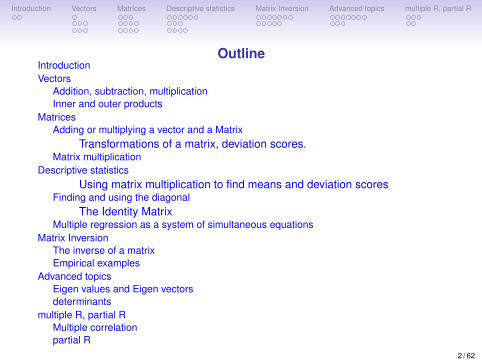
OutlineIntroductionVectors
Addition, subtraction, multiplicationInner and outer products
MatricesAdding or multiplying a vector and a Matrix
Transformations of a matrix, deviation scores.Matrix multiplication
Descriptive statisticsUsing matrix multiplication to find means and deviation scores
Finding and using the diagonalThe Identity Matrix
Multiple regression as a system of simultaneous equationsMatrix Inversion
The inverse of a matrixEmpirical examples
Advanced topicsEigen values and Eigen vectorsdeterminants
multiple R, partial RMultiple correlationpartial R
2 / 62
Introduction Vectors Matrices Descriptive statistics Matrix Inversion Advanced topics multiple R, partial R
Why linear algebra?
• Linear algebra is the fundamental notational technique usedin multiple correlation, factor analysis, and structural equationmodeling• Although it is possible to do psychometrics and statistics
without understanding linear algebra, it is helpful to do so.• Linear algebra is a convenient notational system that allows
us to think about data at a higher (broader) level rather thandata point by data point.• Commercial stats programs do their calculations in linear
algebra but “protect” the user from their seeming complexity.• Some instructors of statistics think it is better to not show the
basic principles used in the analysis and instead perform“cookbook" exercises.• I do not.
3 / 62
Introduction Vectors Matrices Descriptive statistics Matrix Inversion Advanced topics multiple R, partial R
Linear Algebra
• Matrices were used by the Babylonians and Chinese (ca. 100BCE) to do basic calculations and solve simultaneousequations but were not introduced in Western mathematicsuntil the early 19th century.• Introduced to psychologists by Thurstone in 1933 who had
learned about them from a mathematician colleague.• Until then, all analysis was done on “tables” with fairly
laborious ad hoc procedures.
• Matrices may be thought of as “spreadsheets” but with theirown algebra.• Most modern statistics are actually performed by applying
basic principles of linear algebra.• R is explicit in its use of matrices, so am I.
4 / 62
Introduction Vectors Matrices Descriptive statistics Matrix Inversion Advanced topics multiple R, partial R
Scalars, Vectors and Matrices
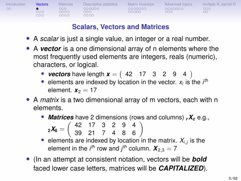
• A scalar is just a single value, an integer or a real number.• A vector is a one dimensional array of n elements where the
most frequently used elements are integers, reals (numeric),characters, or logical.• vectors have length x =
(42 17 3 2 9 4
)• elements are indexed by location in the vector. xi is the i th
element. x2 = 17• A matrix is a two dimensional array of m vectors, each with n
elements.• Matrices have 2 dimensions (rows and columns) r Xc e.g.,
2X6 =
(42 17 3 2 9 439 21 7 4 8 6
)• elements are indexed by location in the matrix. Xi,j is the
element in the i th row and j th column. X 2,3 = 7
• (In an attempt at consistent notation, vectors will be boldfaced lower case letters, matrices will be CAPITALIZED).
5 / 62
Introduction Vectors Matrices Descriptive statistics Matrix Inversion Advanced topics multiple R, partial R
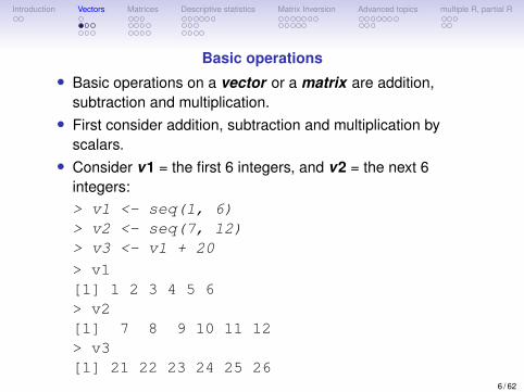
Basic operations• Basic operations on a vector or a matrix are addition,
subtraction and multiplication.• First consider addition, subtraction and multiplication by
scalars.• Consider v1 = the first 6 integers, and v2 = the next 6
integers:> v1 <- seq(1, 6)> v2 <- seq(7, 12)> v3 <- v1 + 20
> v1[1] 1 2 3 4 5 6> v2[1] 7 8 9 10 11 12> v3[1] 21 22 23 24 25 26
6 / 62
Introduction Vectors Matrices Descriptive statistics Matrix Inversion Advanced topics multiple R, partial R
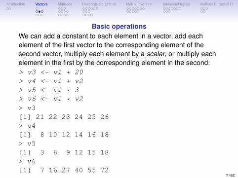
Basic operationsWe can add a constant to each element in a vector, add eachelement of the first vector to the corresponding element of thesecond vector, multiply each element by a scalar, or multiply eachelement in the first by the corresponding element in the second:> v3 <- v1 + 20> v4 <- v1 + v2> v5 <- v1 * 3> v6 <- v1 * v2> v3[1] 21 22 23 24 25 26> v4[1] 8 10 12 14 16 18> v5[1] 3 6 9 12 15 18> v6[1] 7 16 27 40 55 72
7 / 62
Introduction Vectors Matrices Descriptive statistics Matrix Inversion Advanced topics multiple R, partial R
row and column vectors and the transpose operator
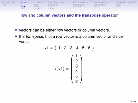
• vectors can be either row vectors or column vectors.• the transpose, t, of a row vector is a column vector and vice
versa
v1 =(
1 2 3 4 5 6)
t(v1) =
123456
8 / 62
Introduction Vectors Matrices Descriptive statistics Matrix Inversion Advanced topics multiple R, partial R
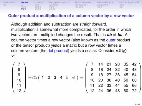
Outer product = multiplication of a column vector by a row vector
Although addition and subtraction are straightforward,multiplication is somewhat more complicated, for the order in whichtwo vectors are multiplied changes the result. That is ab 6= ba. Acolumn vector times a row vector (also known as the outer productor the tensor product) yields a matrix but a row vector times acolumn vectors (the dot product) yields a scalar. Consider v2
⊗v1
789101112
%∗%(
1 2 3 4 5 6)
=
7 14 21 28 35 428 16 24 32 40 489 18 27 36 45 5410 20 30 40 50 6011 22 33 44 55 6612 24 36 48 60 72
9 / 62
Introduction Vectors Matrices Descriptive statistics Matrix Inversion Advanced topics multiple R, partial R
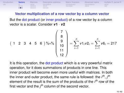
Vector multiplication of a row vector by a column vector
But the dot product (or inner product) of a row vector by a columnvector is a scalar. Consider v1 · v2
(1 2 3 4 5 6
)%∗%
789101112
=n∑
i=1
v1iv2i =n∑
i=1
v6i = 217
It is this operation, the dot product which is a very powerful matrixoperation, for it does summations of products in one line. Thisinner product will become even more useful with matrices. In boththe inner and outer product, the same rule is followed: the i th, j th
element of the result is the sum of the products of the i th row of thefirst vector and the j th column of the second vector.
10 / 62
Introduction Vectors Matrices Descriptive statistics Matrix Inversion Advanced topics multiple R, partial R
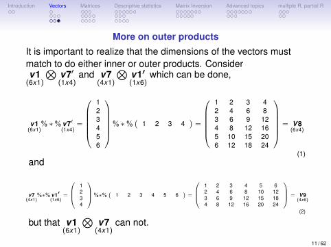
More on outer products
It is important to realize that the dimensions of the vectors mustmatch to do either inner or outer products. Considerv1(6x1)
⊗v7′(1x4)
and v7(4x1)
⊗v1′(1x6)
which can be done,
v1(6x1)
% ∗% v7′(1x4)
=
123456
% ∗%(
1 2 3 4)=
1 2 3 42 4 6 83 6 9 124 8 12 165 10 15 206 12 18 24
= V8(6x4)
(1)and
v7(4x1)
%∗% v1′(1x6)
=
1234
%∗%(
1 2 3 4 5 6)=
1 2 3 4 5 62 4 6 8 10 123 6 9 12 15 184 8 12 16 20 24
= V9(4x6)
(2)
but that v1(6x1)
⊗v7(4x1)
can not.
11 / 62
Introduction Vectors Matrices Descriptive statistics Matrix Inversion Advanced topics multiple R, partial R
Matrices and data
• A matrix is just a two dimensional (rectangular) organizationof numbers.• It is a vector of vectors.
• For data analysis, the typical data matrix is organized withrows containing the responses of a particular subject and thecolumns representing different variables.• Thus, a 6 x 4 data matrix (6 rows, 4 columns) would contain
the data of 6 subjects on 4 different variables.
• In the example below the matrix operation has taken thenumbers 1 through 24 and organized them column wise. Thatis, a matrix is just a way (and a very convenient one at that) oforganizing a data vector in a way that highlights thecorrespondence of multiple observations for the sameindividual. (The matrix is an ordered n-tuplet where n is thenumber of columns).
12 / 62
Introduction Vectors Matrices Descriptive statistics Matrix Inversion Advanced topics multiple R, partial R
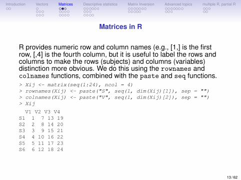
Matrices in R
R provides numeric row and column names (e.g., [1,] is the firstrow, [,4] is the fourth column, but it is useful to label the rows andcolumns to make the rows (subjects) and columns (variables)distinction more obvious. We do this using the rownames andcolnames functions, combined with the paste and seq functions.> Xij <- matrix(seq(1:24), ncol = 4)> rownames(Xij) <- paste("S", seq(1, dim(Xij)[1]), sep = "")> colnames(Xij) <- paste("V", seq(1, dim(Xij)[2]), sep = "")> Xij
V1 V2 V3 V4S1 1 7 13 19S2 2 8 14 20S3 3 9 15 21S4 4 10 16 22S5 5 11 17 23S6 6 12 18 24
13 / 62
Introduction Vectors Matrices Descriptive statistics Matrix Inversion Advanced topics multiple R, partial R
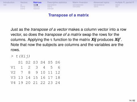
Transpose of a matrix
Just as the transpose of a vector makes a column vector into a rowvector, so does the transpose of a matrix swap the rows for thecolumns. Applying the t function to the matrix Xij produces Xij ′.Note that now the subjects are columns and the variables are therows.
> t(Xij)
S1 S2 S3 S4 S5 S6V1 1 2 3 4 5 6V2 7 8 9 10 11 12V3 13 14 15 16 17 18V4 19 20 21 22 23 24
14 / 62
Introduction Vectors Matrices Descriptive statistics Matrix Inversion Advanced topics multiple R, partial R
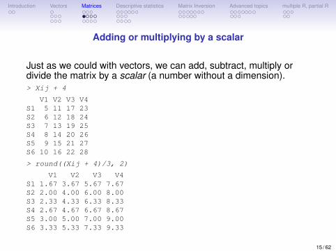
Adding or multiplying by a scalar
Just as we could with vectors, we can add, subtract, multiply ordivide the matrix by a scalar (a number without a dimension).> Xij + 4
V1 V2 V3 V4S1 5 11 17 23S2 6 12 18 24S3 7 13 19 25S4 8 14 20 26S5 9 15 21 27S6 10 16 22 28
> round((Xij + 4)/3, 2)
V1 V2 V3 V4S1 1.67 3.67 5.67 7.67S2 2.00 4.00 6.00 8.00S3 2.33 4.33 6.33 8.33S4 2.67 4.67 6.67 8.67S5 3.00 5.00 7.00 9.00S6 3.33 5.33 7.33 9.33
15 / 62
Introduction Vectors Matrices Descriptive statistics Matrix Inversion Advanced topics multiple R, partial R
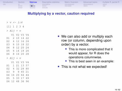
Multiplying by a vector, caution required
> v <- 1:4
[1] 1 2 3 4
> Xij + v
V1 V2 V3 V4S1 2 10 14 22S2 4 12 16 24S3 6 10 18 22S4 8 12 20 24S5 6 14 18 26S6 8 16 20 28
> Xij * v
V1 V2 V3 V4S1 1 21 13 57S2 4 32 28 80S3 9 9 45 21S4 16 20 64 44S5 5 33 17 69S6 12 48 36 96
• We can also add or multiply eachrow (or column, depending uponorder) by a vector.• This is more complicated that it
would appear, for R does theoperations columnwise.
• This is best seen in an example:
• This is not what we expected!
16 / 62
Introduction Vectors Matrices Descriptive statistics Matrix Inversion Advanced topics multiple R, partial R
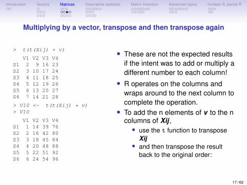
Multiplying by a vector, transpose and then transpose again
> t(t(Xij) + v)
V1 V2 V3 V4S1 2 9 16 23S2 3 10 17 24S3 4 11 18 25S4 5 12 19 26S5 6 13 20 27S6 7 14 21 28
> V10 <- t(t(Xij) * v)> V10
V1 V2 V3 V4S1 1 14 39 76S2 2 16 42 80S3 3 18 45 84S4 4 20 48 88S5 5 22 51 92S6 6 24 54 96
• These are not the expected resultsif the intent was to add or multiply adifferent number to each column!• R operates on the columns and
wraps around to the next column tocomplete the operation.• To add the n elements of v to the n
columns of Xij ,• use the t function to transpose
Xij• and then transpose the result
back to the original order:
17 / 62
Introduction Vectors Matrices Descriptive statistics Matrix Inversion Advanced topics multiple R, partial R
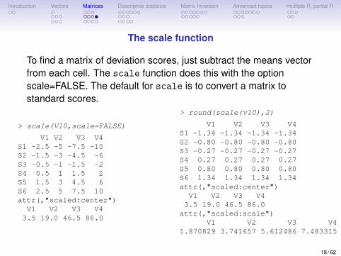
The scale function
To find a matrix of deviation scores, just subtract the means vectorfrom each cell. The scale function does this with the optionscale=FALSE. The default for scale is to convert a matrix tostandard scores.
> scale(V10,scale=FALSE)
V1 V2 V3 V4S1 -2.5 -5 -7.5 -10S2 -1.5 -3 -4.5 -6S3 -0.5 -1 -1.5 -2S4 0.5 1 1.5 2S5 1.5 3 4.5 6S6 2.5 5 7.5 10attr(,"scaled:center")V1 V2 V3 V43.5 19.0 46.5 86.0
> round(scale(v10),2)
V1 V2 V3 V4S1 -1.34 -1.34 -1.34 -1.34S2 -0.80 -0.80 -0.80 -0.80S3 -0.27 -0.27 -0.27 -0.27S4 0.27 0.27 0.27 0.27S5 0.80 0.80 0.80 0.80S6 1.34 1.34 1.34 1.34attr(,"scaled:center")V1 V2 V3 V43.5 19.0 46.5 86.0attr(,"scaled:scale")
V1 V2 V3 V41.870829 3.741657 5.612486 7.483315
18 / 62
Introduction Vectors Matrices Descriptive statistics Matrix Inversion Advanced topics multiple R, partial R
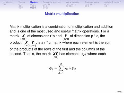
Matrix multiplication
Matrix multiplication is a combination of multiplication and additionand is one of the most used and useful matrix operations. For amatrix X
(rxp)of dimensions r*p and Y
(pxc)of dimension p * c, the
product, X(rxp)
Y(pxc)
, is a r * c matrix where each element is the sum
of the products of the rows of the first and the columns of thesecond. That is, the matrix XY
(rxc)has elements xyij where each
xyij =n∑
k=1
xik ∗ ykj
19 / 62
Introduction Vectors Matrices Descriptive statistics Matrix Inversion Advanced topics multiple R, partial R
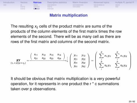
Matrix multiplication
The resulting xij cells of the product matrix are sums of theproducts of the column elements of the first matrix times the rowelements of the second. There will be as many cell as there arerows of the first matrix and columns of the second matrix.
XY(rx x p)(p x cy )
=
(x11 x12 x13 x14x21 x22 x23 x24
)−−−−−−−−−−−−−−−−−−−−→
|↓
y11 y12y21 y22y31 y32y41 y42
=
p∑i
x1i yi1
p∑i
x1i yi2
p∑i
x2i yi1
p∑i
x2i yi2
It should be obvious that matrix multiplication is a very powerfuloperation, for it represents in one product the r * c summationstaken over p observations.
20 / 62
Introduction Vectors Matrices Descriptive statistics Matrix Inversion Advanced topics multiple R, partial R
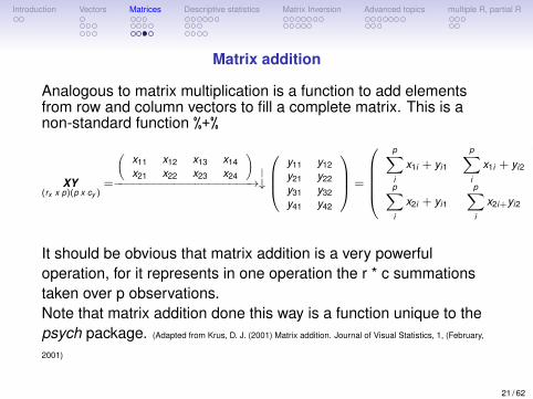
Matrix addition
Analogous to matrix multiplication is a function to add elementsfrom row and column vectors to fill a complete matrix. This is anon-standard function %+%
XY(rx x p)(p x cy )
=
(x11 x12 x13 x14x21 x22 x23 x24
)−−−−−−−−−−−−−−−−−−−−→
|↓
y11 y12y21 y22y31 y32y41 y42
=
p∑i
x1i + yi1
p∑i
x1i + yi2
p∑i
x2i + yi1
p∑i
x2i+yi2
It should be obvious that matrix addition is a very powerfuloperation, for it represents in one operation the r * c summationstaken over p observations.Note that matrix addition done this way is a function unique to thepsych package. (Adapted from Krus, D. J. (2001) Matrix addition. Journal of Visual Statistics, 1, (February,
2001)
21 / 62
Introduction Vectors Matrices Descriptive statistics Matrix Inversion Advanced topics multiple R, partial R
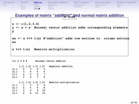
Examples of matrix “addition" and normal matrix additionR code
x <- c(1,2,3,4)y <- x + x #normal vector addition adds corresponding elementsy
xx <- x %+% t(x) #"addition" adds row entries to column entriesxx
x %*% t(x) #matrix multiplication
[1] 2 4 6 8 #normal vector addtion
[,1] [,2] [,3] [,4] #special addition[1,] 2 3 4 5[2,] 3 4 5 6[3,] 4 5 6 7[4,] 5 6 7 8
[,1] [,2] [,3] [,4] #matrix multiplication[1,] 1 2 3 4[2,] 2 4 6 8[3,] 3 6 9 12[4,] 4 8 12 16
22 / 62
Introduction Vectors Matrices Descriptive statistics Matrix Inversion Advanced topics multiple R, partial R
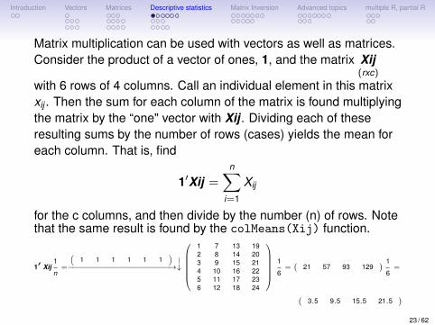
Matrix multiplication can be used with vectors as well as matrices.Consider the product of a vector of ones, 1, and the matrix Xij
(rxc)with 6 rows of 4 columns. Call an individual element in this matrixxij . Then the sum for each column of the matrix is found multiplyingthe matrix by the “one" vector with Xij . Dividing each of theseresulting sums by the number of rows (cases) yields the mean foreach column. That is, find
1′Xij =n∑
i=1
Xij
for the c columns, and then divide by the number (n) of rows. Notethat the same result is found by the colMeans(Xij) function.
1′ Xij1
n=
(1 1 1 1 1 1
)−−−−−−−−−−−−−−−−−−−−−→
|↓
1 7 13 192 8 14 203 9 15 214 10 16 225 11 17 236 12 18 24
1
6=(
21 57 93 129) 1
6=
(3.5 9.5 15.5 21.5
)23 / 62
Introduction Vectors Matrices Descriptive statistics Matrix Inversion Advanced topics multiple R, partial R
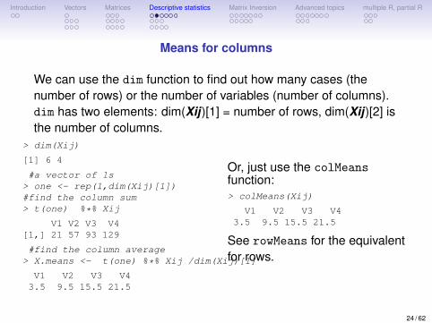
Means for columns
We can use the dim function to find out how many cases (thenumber of rows) or the number of variables (number of columns).dim has two elements: dim(Xij)[1] = number of rows, dim(Xij)[2] isthe number of columns.
> dim(Xij)
[1] 6 4
#a vector of 1s> one <- rep(1,dim(Xij)[1])#find the column sum> t(one) %*% Xij
V1 V2 V3 V4[1,] 21 57 93 129
#find the column average> X.means <- t(one) %*% Xij /dim(Xij)[1]
V1 V2 V3 V43.5 9.5 15.5 21.5
Or, just use the colMeansfunction:> colMeans(Xij)
V1 V2 V3 V43.5 9.5 15.5 21.5
See rowMeans for the equivalentfor rows.
24 / 62
Introduction Vectors Matrices Descriptive statistics Matrix Inversion Advanced topics multiple R, partial R
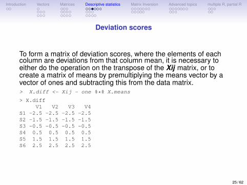
Deviation scores
To form a matrix of deviation scores, where the elements of eachcolumn are deviations from that column mean, it is necessary toeither do the operation on the transpose of the Xij matrix, or tocreate a matrix of means by premultiplying the means vector by avector of ones and subtracting this from the data matrix.> X.diff <- Xij - one %*% X.means
> X.diffV1 V2 V3 V4
S1 -2.5 -2.5 -2.5 -2.5S2 -1.5 -1.5 -1.5 -1.5S3 -0.5 -0.5 -0.5 -0.5S4 0.5 0.5 0.5 0.5S5 1.5 1.5 1.5 1.5S6 2.5 2.5 2.5 2.5
25 / 62
Introduction Vectors Matrices Descriptive statistics Matrix Inversion Advanced topics multiple R, partial R
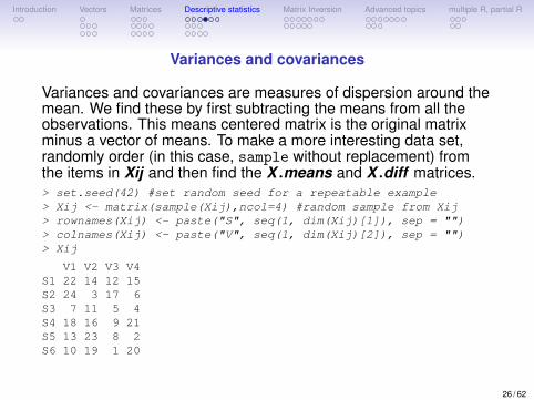
Variances and covariances
Variances and covariances are measures of dispersion around themean. We find these by first subtracting the means from all theobservations. This means centered matrix is the original matrixminus a vector of means. To make a more interesting data set,randomly order (in this case, sample without replacement) fromthe items in Xij and then find the X .means and X .diff matrices.> set.seed(42) #set random seed for a repeatable example> Xij <- matrix(sample(Xij),ncol=4) #random sample from Xij> rownames(Xij) <- paste("S", seq(1, dim(Xij)[1]), sep = "")> colnames(Xij) <- paste("V", seq(1, dim(Xij)[2]), sep = "")> Xij
V1 V2 V3 V4S1 22 14 12 15S2 24 3 17 6S3 7 11 5 4S4 18 16 9 21S5 13 23 8 2S6 10 19 1 20
26 / 62
Introduction Vectors Matrices Descriptive statistics Matrix Inversion Advanced topics multiple R, partial R
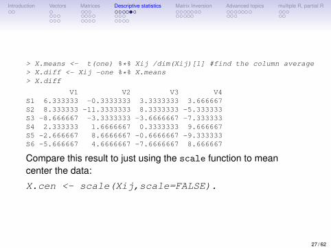
> X.means <- t(one) %*% Xij /dim(Xij)[1] #find the column average> X.diff <- Xij -one %*% X.means> X.diff
V1 V2 V3 V4S1 6.333333 -0.3333333 3.3333333 3.666667S2 8.333333 -11.3333333 8.3333333 -5.333333S3 -8.666667 -3.3333333 -3.6666667 -7.333333S4 2.333333 1.6666667 0.3333333 9.666667S5 -2.666667 8.6666667 -0.6666667 -9.333333S6 -5.666667 4.6666667 -7.6666667 8.666667
Compare this result to just using the scale function to meancenter the data:
X.cen <- scale(Xij,scale=FALSE).
27 / 62
Introduction Vectors Matrices Descriptive statistics Matrix Inversion Advanced topics multiple R, partial R
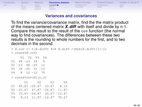
Variances and covariances
To find the variance/covariance matrix, find the the matrix productof the means centered matrix X .diff with itself and divide by n-1.Compare this result to the result of the cov function (the normalway to find covariances). The differences between these tworesults is the rounding to whole numbers for the first, and to twodecimals in the second.> X.cov <- t(X.diff) %*% X.diff /(dim(X.diff)[1]-1)> round(X.cov)
V1 V2 V3 V4V1 46 -23 34 8V2 -23 48 -25 12V3 34 -25 31 -12V4 8 12 -12 70
> round(cov(Xij),2)
V1 V2 V3 V4V1 45.87 -22.67 33.67 8.13V2 -22.67 47.87 -24.87 11.87V3 33.67 -24.87 30.67 -12.47V4 8.13 11.87 -12.47 70.27
28 / 62
Introduction Vectors Matrices Descriptive statistics Matrix Inversion Advanced topics multiple R, partial R
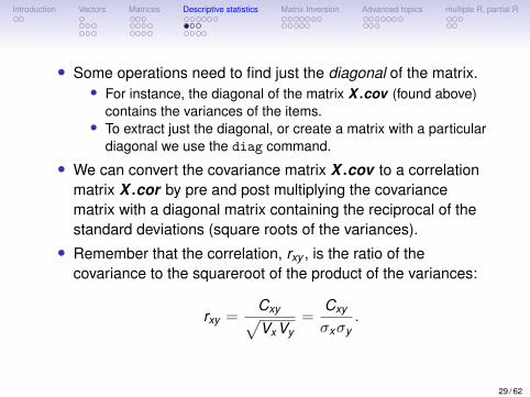
• Some operations need to find just the diagonal of the matrix.• For instance, the diagonal of the matrix X .cov (found above)
contains the variances of the items.• To extract just the diagonal, or create a matrix with a particular
diagonal we use the diag command.
• We can convert the covariance matrix X .cov to a correlationmatrix X .cor by pre and post multiplying the covariancematrix with a diagonal matrix containing the reciprocal of thestandard deviations (square roots of the variances).• Remember that the correlation, rxy , is the ratio of the
covariance to the squareroot of the product of the variances:
rxy =Cxy√VxVy
=Cxy
σxσy.
29 / 62
Introduction Vectors Matrices Descriptive statistics Matrix Inversion Advanced topics multiple R, partial R
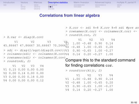
Correlations from linear algebra
> X.var <- diag(X.cov)
V1 V2 V3 V445.86667 47.86667 30.66667 70.26667
> sdi <- diag(1/sqrt(diag(X.cov)))> colnames(sdi) <- colnames(X.cov)> rownames(sdi) <- colnames(X.cov)> round(sdi, 2)
V1 V2 V3 V4V1 0.15 0.00 0.00 0.00V2 0.00 0.14 0.00 0.00V3 0.00 0.00 0.18 0.00V4 0.00 0.00 0.00 0.12
> X.cor <- sdi %*% X.cov %*% sdi #pre and post multiply by 1/sd> rownames(X.cor) <- colnames(X.cor) <- colnames(X.cov)> round(X.cor, 2)
V1 V2 V3 V4V1 1.00 -0.48 0.90 0.14V2 -0.48 1.00 -0.65 0.20V3 0.90 -0.65 1.00 -0.27V4 0.14 0.20 -0.27 1.00
Compare this to the standard commandfor finding correlations cor.> round(cor(Xij), 2)
V1 V2 V3 V4V1 1.00 -0.48 0.90 0.14V2 -0.48 1.00 -0.65 0.20V3 0.90 -0.65 1.00 -0.27V4 0.14 0.20 -0.27 1.00
30 / 62
Introduction Vectors Matrices Descriptive statistics Matrix Inversion Advanced topics multiple R, partial R
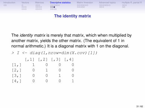
The identity matrix
The identity matrix is merely that matrix, which when multiplied byanother matrix, yields the other matrix. (The equivalent of 1 innormal arithmetic.) It is a diagonal matrix with 1 on the diagonal.
> I <- diag(1,nrow=dim(X.cov)[1])
[,1] [,2] [,3] [,4][1,] 1 0 0 0[2,] 0 1 0 0[3,] 0 0 1 0[4,] 0 0 0 1
31 / 62
Introduction Vectors Matrices Descriptive statistics Matrix Inversion Advanced topics multiple R, partial R
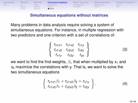
Simultaneous equations without matrices
Many problems in data analysis require solving a system ofsimultaneous equations. For instance, in multiple regression withtwo predictors and one criterion with a set of correlations of:
rx1x1 rx1x2 rx1y
rx1x2 rx2x2 rx2y
rx1y rx2y ryy
(3)
we want to find the find weights, βi , that when multiplied by x1 andx2 maximize the correlations with y. That is, we want to solve thetwo simultaneous equations{
rx1x1β1 + rx1x2β2 = rx1y
rx1x2β1 + rx2x2β2 = rx2y
}. (4)
32 / 62
Introduction Vectors Matrices Descriptive statistics Matrix Inversion Advanced topics multiple R, partial R
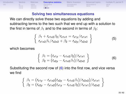
Solving two simultaneous equationsWe can directly solve these two equations by adding andsubtracting terms to the two such that we end up with a solution tothe first in terms of β1 and to the second in terms of β2:{
β1 + rx1x2β2/rx1x1 = rx1y/rx1x1
rx1x2β1/rx2x2 + β2 = rx2y/rx2x2
}(5)
which becomes {β1 = (rx1y − rx1x2β2)/rx1x1
β2 = (rx2y − rx1x2β1)/rx2x2
}(6)
Substituting the second row of (6) into the first row, and vice versawe find{
β1 = (rx1y − rx1x2(rx2y − rx1x2β1)/rx2x2)/rx1x1
β2 = (rx2y − rx1x2(rx1y − rx1x2β2)/rx1x1)/rx2x2
}33 / 62
Introduction Vectors Matrices Descriptive statistics Matrix Inversion Advanced topics multiple R, partial R
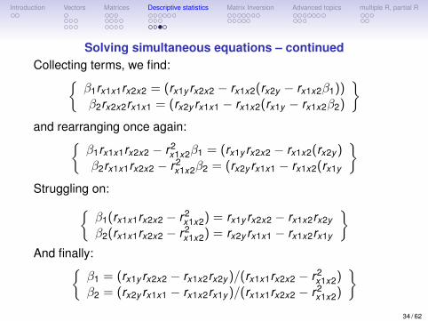
Solving simultaneous equations – continuedCollecting terms, we find:{
β1rx1x1rx2x2 = (rx1y rx2x2 − rx1x2(rx2y − rx1x2β1))β2rx2x2rx1x1 = (rx2y rx1x1 − rx1x2(rx1y − rx1x2β2)
}and rearranging once again:{
β1rx1x1rx2x2 − r2x1x2β1 = (rx1y rx2x2 − rx1x2(rx2y )
β2rx1x1rx2x2 − r2x1x2β2 = (rx2y rx1x1 − rx1x2(rx1y
}Struggling on:{
β1(rx1x1rx2x2 − r2x1x2) = rx1y rx2x2 − rx1x2rx2y
β2(rx1x1rx2x2 − r2x1x2) = rx2y rx1x1 − rx1x2rx1y
}And finally:{
β1 = (rx1y rx2x2 − rx1x2rx2y )/(rx1x1rx2x2 − r2x1x2)
β2 = (rx2y rx1x1 − rx1x2rx1y )/(rx1x1rx2x2 − r2x1x2)
}34 / 62
Introduction Vectors Matrices Descriptive statistics Matrix Inversion Advanced topics multiple R, partial R
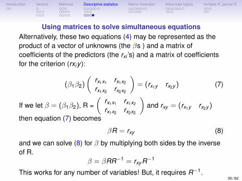
Using matrices to solve simultaneous equationsAlternatively, these two equations (4) may be represented as theproduct of a vector of unknowns (the βs ) and a matrix ofcoefficients of the predictors (the rxi ’s) and a matrix of coefficientsfor the criterion (rxiy ):
(β1β2)
(rx1x1 rx1x2
rx1x2 rx2x2
)= (rx1y rx2y ) (7)
If we let β = (β1β2), R =(
rx1x1 rx1x2
rx1x2 rx2x2
)and rxy = (rx1y rx2y )
then equation (7) becomes
βR = rxy (8)
and we can solve (8) for β by multiplying both sides by the inverseof R.
β = βRR−1 = rxy R−1
This works for any number of variables! But, it requires R−1.35 / 62
Introduction Vectors Matrices Descriptive statistics Matrix Inversion Advanced topics multiple R, partial R
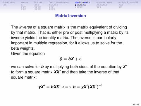
Matrix Inversion
The inverse of a square matrix is the matrix equivalent of dividingby that matrix. That is, either pre or post multiplying a matrix by itsinverse yields the identity matrix. The inverse is particularlyimportant in multiple regression, for it allows us to solve for thebeta weights.Given the equation
y = bX + c
we can solve for b by multiplying both sides of the equation by X ’to form a square matrix XX ′ and then take the inverse of thatsquare matrix:
yX ′ = bXX ′ <=> b = yX ′(XX ′)−1
36 / 62
Introduction Vectors Matrices Descriptive statistics Matrix Inversion Advanced topics multiple R, partial R
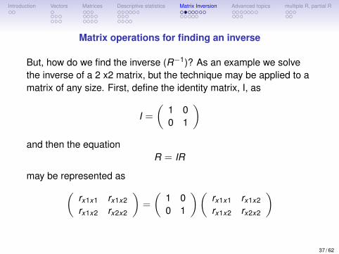
Matrix operations for finding an inverse
But, how do we find the inverse (R−1)? As an example we solvethe inverse of a 2 x2 matrix, but the technique may be applied to amatrix of any size. First, define the identity matrix, I, as
I =
(1 00 1
)and then the equation
R = IR
may be represented as(rx1x1 rx1x2
rx1x2 rx2x2
)=
(1 00 1
)(rx1x1 rx1x2
rx1x2 rx2x2
)
37 / 62
Introduction Vectors Matrices Descriptive statistics Matrix Inversion Advanced topics multiple R, partial R
Transform both sides of the equationDropping the x subscript (for notational simplicity) we have(
r11 r12
r12 r22
)=
(1 00 1
)(r11 r12
r12 r22
)(9)
We may multiply both sides of equation (9) by a simpletransformation matrix (T) without changing the equality. If we dothis repeatedly until the left hand side of equation (9) is the identitymatrix, then the first matrix on the right hand side will be theinverse of R. We do this in several steps to show the process.Let
T1 =
(1
r110
0 1r22
)then we multiply both sides of equation (9) by T1 in order to makethe diagonal elements of the left hand equation = 1 and we have
T1R = T1IR (10)38 / 62
Introduction Vectors Matrices Descriptive statistics Matrix Inversion Advanced topics multiple R, partial R
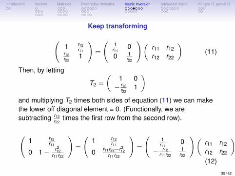
Keep transforming
(1 r12
r11r12r22
1
)=
(1
r110
0 1r22
)(r11 r12
r12 r22
)(11)
Then, by letting
T2 =
(1 0− r12
r221
)and multiplying T2 times both sides of equation (11) we can makethe lower off diagonal element = 0. (Functionally, we aresubtracting r12
r22times the first row from the second row).
(1 r12
r11
0 1− r212
r11r22
)=
(1 r12
r11
0 r11r22−r212
r11r22
)=
(1
r110
− r12r11r22
1r22
)(r11 r12
r12 r22
)(12)
39 / 62
Introduction Vectors Matrices Descriptive statistics Matrix Inversion Advanced topics multiple R, partial R
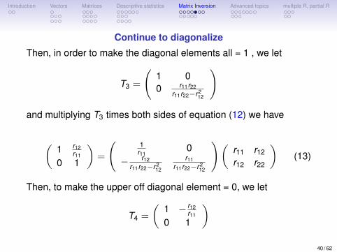
Continue to diagonalize
Then, in order to make the diagonal elements all = 1 , we let
T3 =
(1 00 r11r22
r11r22−r212
)
and multiplying T3 times both sides of equation (12) we have
(1 r12
r11
0 1
)=
(1
r110
− r12r11r22−r2
12
r11r11r22−r2
12
)(r11 r12
r12 r22
)(13)
Then, to make the upper off diagonal element = 0, we let
T4 =
(1 − r12
r11
0 1
)40 / 62
Introduction Vectors Matrices Descriptive statistics Matrix Inversion Advanced topics multiple R, partial R
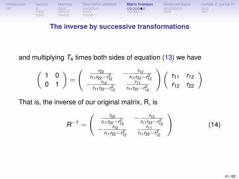
The inverse by successive transformations
and multiplying T4 times both sides of equation (13) we have(1 00 1
)=
( r22r11r22−r2
12− r12
r11r22−r212
− r12r11r22−r2
12
r11r11r22−r2
12
)(r11 r12
r12 r22
)That is, the inverse of our original matrix, R, is
R−1 =
( r22r11r22−r2
12− r12
r11r22−r212
− r12r11r22−r2
12
r11r11r22−r2
12
)(14)
41 / 62
Introduction Vectors Matrices Descriptive statistics Matrix Inversion Advanced topics multiple R, partial R
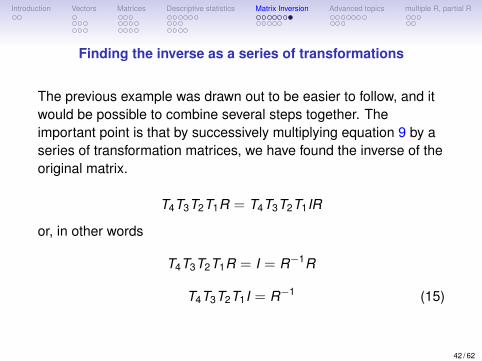
Finding the inverse as a series of transformations
The previous example was drawn out to be easier to follow, and itwould be possible to combine several steps together. Theimportant point is that by successively multiplying equation 9 by aseries of transformation matrices, we have found the inverse of theoriginal matrix.
T4T3T2T1R = T4T3T2T1IR
or, in other words
T4T3T2T1R = I = R−1R
T4T3T2T1I = R−1 (15)
42 / 62
Introduction Vectors Matrices Descriptive statistics Matrix Inversion Advanced topics multiple R, partial R
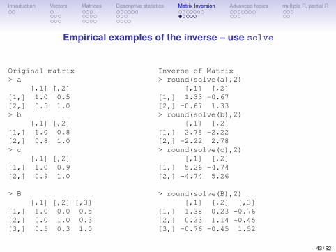
Empirical examples of the inverse – use solve
Original matrix> a
[,1] [,2][1,] 1.0 0.5[2,] 0.5 1.0> b
[,1] [,2][1,] 1.0 0.8[2,] 0.8 1.0> c
[,1] [,2][1,] 1.0 0.9[2,] 0.9 1.0
> B[,1] [,2] [,3]
[1,] 1.0 0.0 0.5[2,] 0.0 1.0 0.3[3,] 0.5 0.3 1.0
Inverse of Matrix> round(solve(a),2)
[,1] [,2][1,] 1.33 -0.67[2,] -0.67 1.33> round(solve(b),2)
[,1] [,2][1,] 2.78 -2.22[2,] -2.22 2.78> round(solve(c),2)
[,1] [,2][1,] 5.26 -4.74[2,] -4.74 5.26
> round(solve(B),2)[,1] [,2] [,3]
[1,] 1.38 0.23 -0.76[2,] 0.23 1.14 -0.45[3,] -0.76 -0.45 1.52
43 / 62
Introduction Vectors Matrices Descriptive statistics Matrix Inversion Advanced topics multiple R, partial R
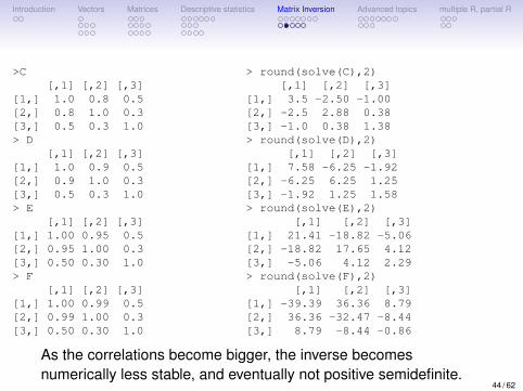
>C[,1] [,2] [,3]
[1,] 1.0 0.8 0.5[2,] 0.8 1.0 0.3[3,] 0.5 0.3 1.0> D
[,1] [,2] [,3][1,] 1.0 0.9 0.5[2,] 0.9 1.0 0.3[3,] 0.5 0.3 1.0> E
[,1] [,2] [,3][1,] 1.00 0.95 0.5[2,] 0.95 1.00 0.3[3,] 0.50 0.30 1.0> F
[,1] [,2] [,3][1,] 1.00 0.99 0.5[2,] 0.99 1.00 0.3[3,] 0.50 0.30 1.0
> round(solve(C),2)[,1] [,2] [,3]
[1,] 3.5 -2.50 -1.00[2,] -2.5 2.88 0.38[3,] -1.0 0.38 1.38> round(solve(D),2)
[,1] [,2] [,3][1,] 7.58 -6.25 -1.92[2,] -6.25 6.25 1.25[3,] -1.92 1.25 1.58> round(solve(E),2)
[,1] [,2] [,3][1,] 21.41 -18.82 -5.06[2,] -18.82 17.65 4.12[3,] -5.06 4.12 2.29> round(solve(F),2)
[,1] [,2] [,3][1,] -39.39 36.36 8.79[2,] 36.36 -32.47 -8.44[3,] 8.79 -8.44 -0.86
As the correlations become bigger, the inverse becomesnumerically less stable, and eventually not positive semidefinite.
44 / 62
Introduction Vectors Matrices Descriptive statistics Matrix Inversion Advanced topics multiple R, partial R
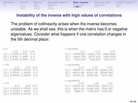
Instability of the inverse with high values of correlations
The problem of collinearity arises when the inverse becomesunstable. As we shall see, this is when the matrix has 0 or negativeeigenvalues. Consider what happens if one correlation changes inthe 5th decimal place:
> F[,1] [,2] [,3]
[1,] 1.0000 0.9761 0.5[2,] 0.9761 1.0000 0.3[3,] 0.5000 0.3000 1.0
> F2[,1] [,2] [,3]
[1,] 1.00000 0.97613 0.5[2,] 0.97613 1.00000 0.3[3,] 0.50000 0.30000 1.0
> F3[,1] [,2] [,3]
[1,] 1.00000 0.97615 0.5[2,] 0.97615 1.00000 0.3[3,] 0.50000 0.30000 1.0
> solve(F)[,1] [,2] [,3]
[1,] 15478.823 -14051.709 -3523.8986[2,] -14051.709 12757.272 3198.6732[3,] -3523.899 3198.673 803.3473
> solve(F2)[,1] [,2] [,3]
[1,] 98665.31 -89571.84 -22461.103[2,] -89571.84 81317.56 20390.650[3,] -22461.10 20390.65 5114.357
> solve(F3)[,1] [,2] [,3]
[1,] -38199.18 34679.400 8695.771[2,] 34679.40 -31482.842 -7894.847[3,] 8695.77 -7894.847 -1978.431
45 / 62
Introduction Vectors Matrices Descriptive statistics Matrix Inversion Advanced topics multiple R, partial R
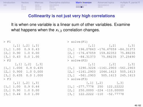
Collinearity is not just very high correlations
It is when one variable is a linear sum of other variables. Examinewhat happens when the x1,3 correlation changes.
> F1[,1] [,2] [,3]
[1,] 1.00 0.9 0.43[2,] 0.90 1.0 0.00[3,] 0.43 0.0 1.00> F2
[,1] [,2] [,3][1,] 1.000 0.9 0.435[2,] 0.900 1.0 0.000[3,] 0.435 0.0 1.000> F3
[,1] [,2] [,3][1,] 1.00 0.9 0.44[2,] 0.90 1.0 0.00[3,] 0.44 0.0 1.00
> solve(F1)[,1] [,2] [,3]
[1,] 196.07843 -176.47059 -84.31373[2,] -176.47059 159.82353 75.88235[3,] -84.31373 75.88235 37.25490> solve(F2)
[,1] [,2] [,3][1,] 1290.3226 -1161.2903 -561.2903[2,] -1161.2903 1046.1613 505.1613[3,] -561.2903 505.1613 245.1613> solve(F3)
[,1] [,2] [,3][1,] -277.7778 250 122.22222[2,] 250.0000 -224 -110.00000[3,] 122.2222 -110 -52.77778
46 / 62
Introduction Vectors Matrices Descriptive statistics Matrix Inversion Advanced topics multiple R, partial R
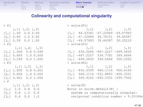
Colinearity and computational singularity
> F1[,1] [,2] [,3]
[1,] 1.00 0.8 0.59[2,] 0.80 1.0 0.00[3,] 0.59 0.0 1.00> F2
[,1] [,2] [,3][1,] 1.000 0.8 0.599[2,] 0.800 1.0 0.000[3,] 0.599 0.0 1.000> F3
[,1] [,2] [,3][1,] 1.000 0.8 0.601[2,] 0.800 1.0 0.000[3,] 0.601 0.0 1.000> F
[,1] [,2] [,3][1,] 1.0 0.8 0.6[2,] 0.8 1.0 0.0[3,] 0.6 0.0 1.0
> solve(F1)[,1] [,2] [,3]
[1,] 84.03361 -67.22689 -49.57983[2,] -67.22689 54.78151 39.66387[3,] -49.57983 39.66387 30.25210> solve(F2)
[,1] [,2] [,3][1,] 834.0284 -667.2227 -499.5830[2,] -667.2227 534.7781 399.6664[3,] -499.5830 399.6664 300.2502> solve(F2)
[,1] [,2] [,3][1,] -832.6395 666.1116 500.4163[2,] 666.1116 -531.8893 -400.3331[3,] 500.4163 -400.3331 -299.7502
> solve(F)Error in solve.default(F) :
system is computationally singular:reciprocal condition number = 9.25186e-18
47 / 62
Introduction Vectors Matrices Descriptive statistics Matrix Inversion Advanced topics multiple R, partial R
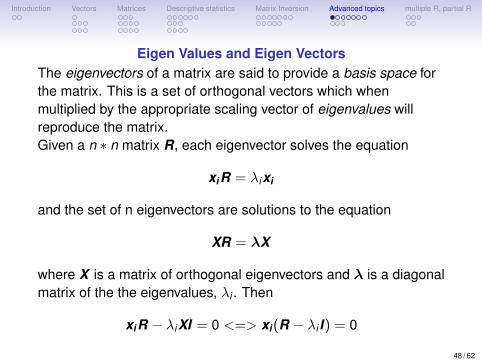
Eigen Values and Eigen VectorsThe eigenvectors of a matrix are said to provide a basis space forthe matrix. This is a set of orthogonal vectors which whenmultiplied by the appropriate scaling vector of eigenvalues willreproduce the matrix.Given a n ∗ n matrix R, each eigenvector solves the equation
xiR = λixi
and the set of n eigenvectors are solutions to the equation
XR = λX
where X is a matrix of orthogonal eigenvectors and λ is a diagonalmatrix of the the eigenvalues, λi . Then
xiR − λiXI = 0 <=> xi(R − λi I) = 0
48 / 62
Introduction Vectors Matrices Descriptive statistics Matrix Inversion Advanced topics multiple R, partial R
Finding eigen values
Finding the eigenvectors and values is computationally tedious, butmay be done using the eigen function which uses a QRdecomposition of the matrix. That the vectors making up X areorthogonal means that
XX ′ = I
and because they form the basis space for R that
R = XλX ′.
That is, it is possible to recreate the correlation matrix R in terms ofan orthogonal set of vectors (the eigenvectors) scaled by theirassociated eigenvalues.
49 / 62
Introduction Vectors Matrices Descriptive statistics Matrix Inversion Advanced topics multiple R, partial R
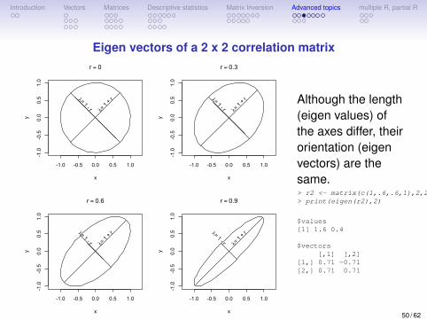
Eigen vectors of a 2 x 2 correlation matrix
-1.0 -0.5 0.0 0.5 1.0
-1.0
-0.5
0.0
0.5
1.0
r = 0
x
y
λ= 1
+ rλ= 1 - r
-1.0 -0.5 0.0 0.5 1.0-1.0
-0.5
0.0
0.5
1.0
r = 0.3
x
y
λ= 1
+ rλ= 1 - r
-1.0 -0.5 0.0 0.5 1.0
-1.0
-0.5
0.0
0.5
1.0
r = 0.6
x
y
λ= 1
+ rλ= 1 - r
-1.0 -0.5 0.0 0.5 1.0
-1.0
-0.5
0.0
0.5
1.0
r = 0.9
x
y
λ= 1
+ rλ= 1 - r
Although the length(eigen values) ofthe axes differ, theirorientation (eigenvectors) are thesame.> r2 <- matrix(c(1,.6,.6,1),2,2)> print(eigen(r2),2)
$values[1] 1.6 0.4
$vectors[,1] [,2]
[1,] 0.71 -0.71[2,] 0.71 0.71
50 / 62
Introduction Vectors Matrices Descriptive statistics Matrix Inversion Advanced topics multiple R, partial R
Eigenvalue decomposition and matrix inverses
1. A correlation matrix can be recreated by its (orthogonal)eigenvectors and eigen values• R = XλX ′ where• XX ′ = I = X ′X the eigenvectors are orthogonal.
2. The inverse of a matrix R−1 is that matrix which whenmultiplied by R is the Identify matrix I .• RR−1 = R−1R = I
3. Combine these two concepts and we see that the inverse isX (1/λ)X ′ since• RR−1 = (XλX ′)(X (1/λ)X ′) = (Xλ)(X ′X )(1/λ)X ′)• (Xλ)I(1/λ)X ′) = X(λI(1/λ)X ′ = XIX ′ = I
4. Thus, the problem of a non-semidefinite matrix is really aproblem of 0 or negative eigen values.
51 / 62
Introduction Vectors Matrices Descriptive statistics Matrix Inversion Advanced topics multiple R, partial R
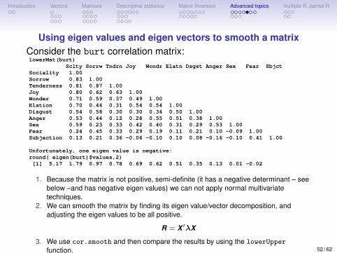
Using eigen values and eigen vectors to smooth a matrixConsider the burt correlation matrix:lowerMat(burt)
Sclty Sorrw Tndrn Joy Wondr Elatn Dsgst Anger Sex Fear SbjctSociality 1.00Sorrow 0.83 1.00Tenderness 0.81 0.87 1.00Joy 0.80 0.62 0.63 1.00Wonder 0.71 0.59 0.37 0.49 1.00Elation 0.70 0.44 0.31 0.54 0.54 1.00Disgust 0.54 0.58 0.30 0.30 0.34 0.50 1.00Anger 0.53 0.44 0.12 0.28 0.55 0.51 0.38 1.00Sex 0.59 0.23 0.33 0.42 0.40 0.31 0.29 0.53 1.00Fear 0.24 0.45 0.33 0.29 0.19 0.11 0.21 0.10 -0.09 1.00Subjection 0.13 0.21 0.36 -0.06 -0.10 0.10 0.08 -0.16 -0.10 0.41 1.00
Unfortunately, one eigen value is negative:round( eigen(burt)$values,2)[1] 5.17 1.79 0.97 0.78 0.69 0.62 0.51 0.35 0.13 0.01 -0.02
1. Because the matrix is not positive, semi-definite (it has a negative determinant – seebelow –and has negative eigen values) we can not apply normal multivariatetechniques.
2. We can smooth the matrix by finding its eigen value/vector decomposition, andadjusting the eigen values to be all positive.
R = X ′λX
3. We use cor.smooth and then compare the results by using the lowerUpper
function. 52 / 62
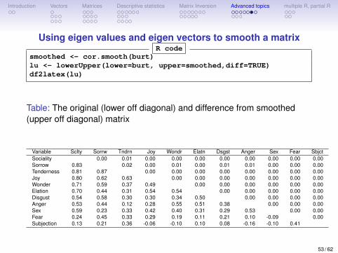
Introduction Vectors Matrices Descriptive statistics Matrix Inversion Advanced topics multiple R, partial R
Using eigen values and eigen vectors to smooth a matrixR code
smoothed <- cor.smooth(burt)lu <- lowerUpper(lower=burt, upper=smoothed,diff=TRUE)df2latex(lu)
Table: The original (lower off diagonal) and difference from smoothed(upper off diagonal) matrix
Variable Sclty Sorrw Tndrn Joy Wondr Elatn Dsgst Anger Sex Fear SbjctSociality 0.00 0.01 0.00 0.00 0.00 0.00 0.00 0.00 0.00 0.00Sorrow 0.83 0.02 0.00 0.01 0.00 0.01 0.01 0.00 0.00 0.00Tenderness 0.81 0.87 0.00 0.00 0.00 0.00 0.00 0.00 0.00 0.00Joy 0.80 0.62 0.63 0.00 0.00 0.00 0.00 0.00 0.00 0.00Wonder 0.71 0.59 0.37 0.49 0.00 0.00 0.00 0.00 0.00 0.00Elation 0.70 0.44 0.31 0.54 0.54 0.00 0.00 0.00 0.00 0.00Disgust 0.54 0.58 0.30 0.30 0.34 0.50 0.00 0.00 0.00 0.00Anger 0.53 0.44 0.12 0.28 0.55 0.51 0.38 0.00 0.00 0.00Sex 0.59 0.23 0.33 0.42 0.40 0.31 0.29 0.53 0.00 0.00Fear 0.24 0.45 0.33 0.29 0.19 0.11 0.21 0.10 -0.09 0.00Subjection 0.13 0.21 0.36 -0.06 -0.10 0.10 0.08 -0.16 -0.10 0.41
53 / 62
Introduction Vectors Matrices Descriptive statistics Matrix Inversion Advanced topics multiple R, partial R
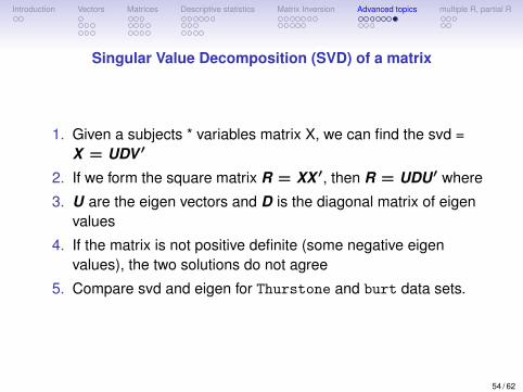
Singular Value Decomposition (SVD) of a matrix
1. Given a subjects * variables matrix X, we can find the svd =X = UDV ′
2. If we form the square matrix R = XX ′, then R = UDU′ where
3. U are the eigen vectors and D is the diagonal matrix of eigenvalues
4. If the matrix is not positive definite (some negative eigenvalues), the two solutions do not agree
5. Compare svd and eigen for Thurstone and burt data sets.
54 / 62
Introduction Vectors Matrices Descriptive statistics Matrix Inversion Advanced topics multiple R, partial R
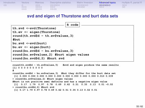
svd and eigen of Thurstone and burt data sets
R codeth.svd <-svd(Thurstone)th.ev <- eigen(Thurstone)round(th.svd$d - th.ev$values,3)#butbu.svd <-svd(burt)bu.ev <- eigen(burt)round(bu.svd$d - bu.ev$values,3)round(bu.ev$values,2) #burt eigen valuesround(bu.svd$d,2) #burt svd
round(th.svd$d - th.ev$values,5) #svd and eigen produce the same results[1] 0 0 0 0 0 0 0 0 0#round(bu.svd$d - bu.ev$values,3) #but they differ for the burt data set[1] 0.000 0.000 0.000 0.000 0.000 0.000 0.000 0.000 0.000 0.010 0.039
> round(bu.ev$values,2) #burt eigen values#Burt is not positive semi definite and has a negative eigen value[1] 5.17 1.79 0.97 0.78 0.69 0.62 0.51 0.35 0.13 0.01 -0.02
> round(bu.svd$d,2) #burt svd[1] 5.17 1.79 0.97 0.78 0.69 0.62 0.51 0.35 0.13 0.02 0.01
55 / 62
Introduction Vectors Matrices Descriptive statistics Matrix Inversion Advanced topics multiple R, partial R
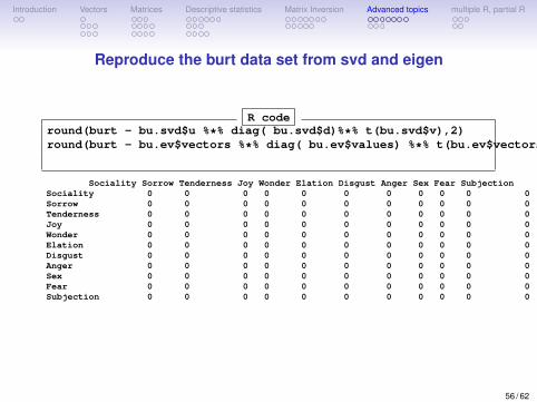
Reproduce the burt data set from svd and eigen
R coderound(burt - bu.svd$u %*% diag( bu.svd$d)%*% t(bu.svd$v),2)round(burt - bu.ev$vectors %*% diag( bu.ev$values) %*% t(bu.ev$vectors),2)
Sociality Sorrow Tenderness Joy Wonder Elation Disgust Anger Sex Fear SubjectionSociality 0 0 0 0 0 0 0 0 0 0 0Sorrow 0 0 0 0 0 0 0 0 0 0 0Tenderness 0 0 0 0 0 0 0 0 0 0 0Joy 0 0 0 0 0 0 0 0 0 0 0Wonder 0 0 0 0 0 0 0 0 0 0 0Elation 0 0 0 0 0 0 0 0 0 0 0Disgust 0 0 0 0 0 0 0 0 0 0 0Anger 0 0 0 0 0 0 0 0 0 0 0Sex 0 0 0 0 0 0 0 0 0 0 0Fear 0 0 0 0 0 0 0 0 0 0 0Subjection 0 0 0 0 0 0 0 0 0 0 0
56 / 62
Introduction Vectors Matrices Descriptive statistics Matrix Inversion Advanced topics multiple R, partial R
Pseudo Inverses are based upon the Singular Value Decomposition ofa matrix
1. A matrix may be decomposed into three matrices X = UDV ′
2. We do this with the svd function
3. The pseudo inverse is UD for positive values of D.
4. Seems to be more robust for finding regressions than simpleinverse.
5. Compare the D value of svd to the eigen values of an eigendecomposition
57 / 62
Introduction Vectors Matrices Descriptive statistics Matrix Inversion Advanced topics multiple R, partial R
Determinants• The determinant of an n * n correlation matrix may be thought
of as the proportion of the possible n-space spanned by thevariable space and is sometimes called the generalizedvariance of the matrix. As such, it can also be considered asthe volume of the variable space.• If the correlation matrix is thought of a representing vectors
within a n dimensional space, then the eigenvalues are thelengths of the axes of that space. The product of these, thedeterminant, is then the volume of the space.• It will be a maximum when the axes are all of unit length and
be zero if at least one axis is zero.• Think of a three dimensional sphere (and then generalize to a
n dimensional hypersphere.)• If it is squashed in a way that preserves the sum of the lengths
of the axes, then volume of the oblate hyper sphere will bereduced.
58 / 62
Introduction Vectors Matrices Descriptive statistics Matrix Inversion Advanced topics multiple R, partial R
Determinants and redundancyThe determinant is an inverse measure of the redundancy of thematrix. The smaller the determinant, the more variables in thematrix are measuring the same thing (are correlated). Thedeterminant of the identity matrix is 1, the determinant of a matrixwith at least two perfectly correlated (linearly dependent) rows orcolumns will be 0. If the matrix is transformed into a lower diagonalmatrix, the determinant is the product of the diagonals. Thedeterminant of a n * n square matrix, R is also the product of the neigenvalues of that matrix.
det(R) = ‖R‖ = Πni=1λi (16)
and the characteristic equation for a square matrix, X , is
‖X − λI‖ = 0
where λi is an eigenvalue of X .59 / 62
Introduction Vectors Matrices Descriptive statistics Matrix Inversion Advanced topics multiple R, partial R
Finding and using the determinant
1. The determinant may be found by the det function.
2. A negative determinant implies the matrix is not positivesemi-definite. It will have negative eigen values.
3. A determinant of 0 means the matrix is not invertible4. The determinant may be used in estimating the goodness of
fit of a particular model (Σ) to the data (S)• for when the model fits perfectly, then the inverse of the model
times the data (Σ−1S) will be an identity matrix and thedeterminant (det(Σ−1S) will be 1.
• A poor model fit will have a determinant much less than 1.• Remember, that the determinant is just the product of the
eigen values
60 / 62
Introduction Vectors Matrices Descriptive statistics Matrix Inversion Advanced topics multiple R, partial R
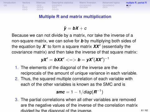
Multiple R and matrix multiplication
y = bX + c
Because we can not divide by a matrix, nor take the inverse of anon-square matrix, we can solve for b by multiplying both sides ofthe equation by X ’ to form a square matrix XX ′ (essentially thecovariance matrix) and then take the inverse of that square matrix:
yX ′ = bXX ′ <=> b = yX ′(XX ′)−1
1. The elements of the diagonal of the inverse are thereciprocals of the amount of unique variance in each variable.
2. Thus, the squared multiple correlation of each variable witheach of the other variables is known as the SMC and is
smc = 1− 1/diag(R−1)
3. The partial correlations when all other variables are removedare the negative values of the inverse of the correlation matrixdivided by the diagonal of the inverse. 61 / 62
Introduction Vectors Matrices Descriptive statistics Matrix Inversion Advanced topics multiple R, partial R
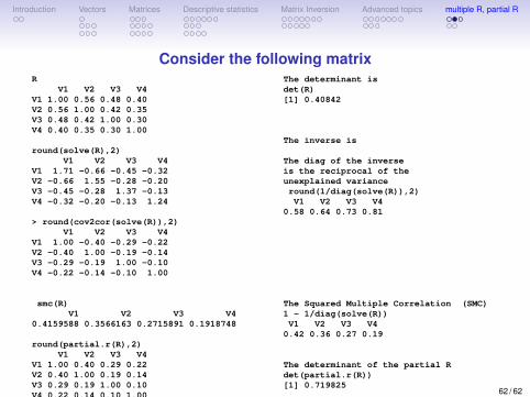
Consider the following matrixR
V1 V2 V3 V4V1 1.00 0.56 0.48 0.40V2 0.56 1.00 0.42 0.35V3 0.48 0.42 1.00 0.30V4 0.40 0.35 0.30 1.00
round(solve(R),2)V1 V2 V3 V4
V1 1.71 -0.66 -0.45 -0.32V2 -0.66 1.55 -0.28 -0.20V3 -0.45 -0.28 1.37 -0.13V4 -0.32 -0.20 -0.13 1.24
> round(cov2cor(solve(R)),2)V1 V2 V3 V4
V1 1.00 -0.40 -0.29 -0.22V2 -0.40 1.00 -0.19 -0.14V3 -0.29 -0.19 1.00 -0.10V4 -0.22 -0.14 -0.10 1.00
smc(R)V1 V2 V3 V4
0.4159588 0.3566163 0.2715891 0.1918748
round(partial.r(R),2)V1 V2 V3 V4
V1 1.00 0.40 0.29 0.22V2 0.40 1.00 0.19 0.14V3 0.29 0.19 1.00 0.10V4 0.22 0.14 0.10 1.00
The determinant isdet(R)[1] 0.40842
The inverse is
The diag of the inverseis the reciprocal of theunexplained varianceround(1/diag(solve(R)),2)V1 V2 V3 V4
0.58 0.64 0.73 0.81
The Squared Multiple Correlation (SMC)1 - 1/diag(solve(R))V1 V2 V3 V4
0.42 0.36 0.27 0.19
The determinant of the partial Rdet(partial.r(R))[1] 0.719825
62 / 62
Introduction Vectors Matrices Descriptive statistics Matrix Inversion Advanced topics multiple R, partial R
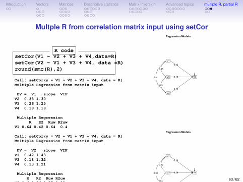
Multple R from correlation matrix input using setCor
R codesetCor(V1 ~ V2 + V3 + V4,data=R)setCor(V2 ~ V1 + V3 + V4, data =R)round(smc(R),2)
Call: setCor(y = V1 ~ V2 + V3 + V4, data = R)Multiple Regression from matrix input
DV = V1 slope VIFV2 0.38 1.30V3 0.26 1.25V4 0.19 1.18
Multiple RegressionR R2 Ruw R2uw
V1 0.64 0.42 0.64 0.4
Call: setCor(y = V2 ~ V1 + V3 + V4, data = R)Multiple Regression from matrix input
DV = V2 slope VIFV1 0.42 1.43V3 0.18 1.32V4 0.13 1.21
Multiple RegressionR R2 Ruw R2uw
V2 0.6 0.36 0.57 0.33
V1 V2 V3 V40.42 0.36 0.27 0.19
Regression Models
V1
V3
V4
V2
0.42
0.18
0.13
0.48
0.4
0.3
Regression Models
V2
V3
V4
V1
0.38
0.26
0.19
0.42
0.35
0.3 63 / 62
Introduction Vectors Matrices Descriptive statistics Matrix Inversion Advanced topics multiple R, partial R
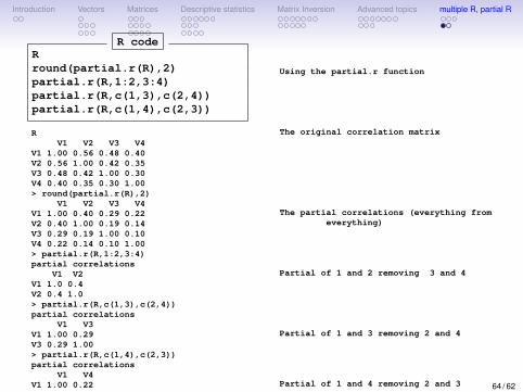
R codeRround(partial.r(R),2)partial.r(R,1:2,3:4)partial.r(R,c(1,3),c(2,4))partial.r(R,c(1,4),c(2,3))
RV1 V2 V3 V4
V1 1.00 0.56 0.48 0.40V2 0.56 1.00 0.42 0.35V3 0.48 0.42 1.00 0.30V4 0.40 0.35 0.30 1.00> round(partial.r(R),2)
V1 V2 V3 V4V1 1.00 0.40 0.29 0.22V2 0.40 1.00 0.19 0.14V3 0.29 0.19 1.00 0.10V4 0.22 0.14 0.10 1.00> partial.r(R,1:2,3:4)partial correlations
V1 V2V1 1.0 0.4V2 0.4 1.0> partial.r(R,c(1,3),c(2,4))partial correlations
V1 V3V1 1.00 0.29V3 0.29 1.00> partial.r(R,c(1,4),c(2,3))partial correlations
V1 V4V1 1.00 0.22V4 0.22 1.00
Using the partial.r function
The original correlation matrix
The partial correlations (everything fromeverything)
Partial of 1 and 2 removing 3 and 4
Partial of 1 and 3 removing 2 and 4
Partial of 1 and 4 removing 2 and 3 64 / 62
Introduction Vectors Matrices Descriptive statistics Matrix Inversion Advanced topics multiple R, partial R
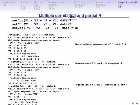
Multiple correlation and partial RR codesetCor(V1 ~ V2 + V3 + V4, data=R)setCor(V1 ~ V2 + V3 - V4, data=R)setCor( V1 ~ V2 - V3 - V4, data = R)
setCor(V1 ~ V2 + V3 + V4, data=R)Call: setCor(y = V1 ~ V2 + V3 + V4, data = R)Multiple Regression from matrix inputDV = V1 slope VIF
V2 0.38 1.30V3 0.26 1.25V4 0.19 1.18Multiple Regression
R R2 Ruw R2uwV1 0.64 0.42 0.64 0.4> setCor(V1 ~ V2 + V3 - V4, data=R)Call: setCor(y = V1 ~ V2 + V3 - V4, data = R)Multiple Regression from matrix inputDV = V1 slope VIF
V2 0.38 1.14V3 0.26 1.14Multiple Regression
R R2 Ruw R2uwV1 0.55 0.3 0.5 0.25> setCor(V1 ~ V2 - V3 - V4, data=R)Call: setCor(y = V1 ~ V2 - V3 - V4, data = R)Multiple Regression from matrix inputDV = V1 slope VIF
V2 0.38 1Multiple Regression
R R2 Ruw R2uwV1 0.4 0.16 0.34 0.11
The complete regression of 1 on 2,3,4
Regression of 1 on 2, 3 removing 4
Regression of 1 on 2, removing 3 and 4
65 / 62