Open Journal of Civil Engineering, 2014, 4, 274-284 Published Online September 2014 in SciRes. http://www.scirp.org/journal/ojce http://dx.doi.org/10.4236/ojce.2014.43023

How to cite this paper: Ndiaye, C., Fall, M., Ndiaye, M., Sangare, D. and Tall, A. (2014) A Review and Update of Analytical and Numerical Solutions of the Terzaghi One-Dimensional Consolidation Equation. Open Journal of Civil Engineering, 4, 274-284. http://dx.doi.org/10.4236/ojce.2014.43023

A Review and Update of Analytical and Numerical Solutions of the Terzaghi One-Dimensional Consolidation Equation Cheikhou Ndiaye1, Meissa Fall1, Mapathe Ndiaye1, Daouda Sangare2, Abib Tall1 1Laboratoire de Mécanique et Modélisation, UFR Sciences de l’Ingénieur, Université de Thiès, Thiès, Sénégal 2Laboratoire d’Analyse Numérique et d’Informatique, UFR Sciences Appliquées et Technologie, Université Gaston Berger, Saint-Louis, Sénégal Email: cheikhou.ndiaye@univ-thies.sn Received 19 June 2014; revised 8 August 2014; accepted 28 August 2014

Copyright © 2014 by authors and Scientific Research Publishing Inc. This work is licensed under the Creative Commons Attribution International License (CC BY). http://creativecommons.org/licenses/by/4.0/

Abstract Practical resolution of consolidation problems that we often face requires an extensive and solid knowledge of the different parameters highlighted by the Terzaghi one-dimensional consolidation theory. This theory, with its assumptions, leads to a partial differential equation of second order in space and first order in time of pore water pressure. Analytical and numerical resolutions of this equation allow determining the water pressure variation before and after the application of a charge. Numerical modeling has enabled the simulation of the whole results obtained by the two methods of resolution (pressure, degree of consolidation, time factor, among others) to have a physical analysis and a lawful observation that lead to a suitable understanding of the phenome-non of Terzaghi one-dimensional consolidation.

Keywords Pore Pressure, Numerical Solution, Analytical Solution, Modeling, Consolidation, Time Factor

1. Introduction The unidimensional consolidation of soils has been described by Terzaghi using partial differential equations [1]. The resolution of these equations can be performed analytically and/or numerically [2] [3]. In this work, we re-solved Terzaghi partial differential equations using Fourier method and finite difference respectively for analyt-ical and numerical solutions. At a further step we used numerical modeling to represent graphically the two so-lutions in order to validate the obtained results.

C. Ndiaye et al.

275

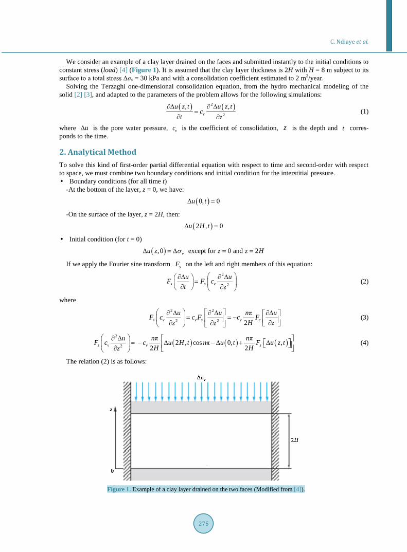
We consider an example of a clay layer drained on the faces and submitted instantly to the initial conditions to constant stress (load) [4] (Figure 1). It is assumed that the clay layer thickness is 2H with H = 8 m subject to its surface to a total stress Δσv = 30 kPa and with a consolidation coefficient estimated to 2 m2/year.

Solving the Terzaghi one-dimensional consolidation equation, from the hydro mechanical modeling of the solid [2] [3], and adapted to the parameters of the problem allows for the following simulations:

( ) ( )2

2

, ,v

u z t u z tc

t z∂∆ ∂ ∆

=∂ ∂

(1)

where u∆ is the pore water pressure, vc is the coefficient of consolidation, z is the depth and t corres-ponds to the time.

2. Analytical Method To solve this kind of first-order partial differential equation with respect to time and second-order with respect to space, we must combine two boundary conditions and initial condition for the interstitial pressure. Boundary conditions (for all time t)

-At the bottom of the layer, z = 0, we have:

( )0, 0u t∆ =

-On the surface of the layer, z = 2H, then:

( )2 , 0u H t∆ =

Initial condition (for t = 0)

( ) except for 0,0 and 2v z zz Hu σ == =∆ ∆

If we apply the Fourier sine transform sF on the left and right members of this equation: 2

2s s vu uF F ct z

∂∆ ∂ ∆ = ∂ ∂ (2)

where 2 2

2 2

π2s v v s v c

u u n uF c c F c FH zz z

∂ ∆ ∂ ∆ ∂∆ = = − ∂∂ ∂ (3)

( ) ( ) ( )2

2

π π 2 , cos π 0, ,2 2s v v s

u n nF c c u H t n u t F u z tH Hz

∂ ∆ = − ∆ − ∆ + ∆ ∂ (4)

The relation (2) is as follows:

Figure 1. Example of a clay layer drained on the two faces (Modified from [4]).

C. Ndiaye et al.

276

( )( )

2, π ,2

sv s

F u z t nc F u z tt H

∂ ∆ = − ∆ ∂ (5)

( ) [ ] ( )[ ]

2 2,π πln , ln 0 ln2 0 2

ss v s v

s

F u z tn nF u z t c t F c tH F H

∆ ∆ = − + ⇒ = − (6)

( )[ ] ( ) [ ]

2 2π π, 2 2

e , 0 e0

v vc cs

s ss

n nt tF u z t H HF u z t F

F

− − ∆ = ⇒ ∆ = (7)

Since the method used is the sine Fourier transform based on the odd frequency (sinusoidal) of the interstitial pressure, the development into Fourier series will not affect the coefficients an.

( )0

π, sin2n

n

n zu z t bH

∞

=

= ∑ (8)

where

( )2 ,2n sb F u z t

H= ∆

By substituting, the equation can be rewritten into this form:

( ) ( ) [ ]

2

0 0

π22 π 1 π, , sin 0 e sin

2 2 2

vc

s sn n

n tHn z n zu z t F u z t F

H H H H

−∞ ∞

= =

∆ = ∆ = ∑ ∑ (9)

[ ] ( ) ( )22 2

00 0

π π 2 π0 ,0 ,0 sin d sin d cos2 2 π 2

HH H

s s v vn z n z H n zF F u z u z z z

H H n Hσ σ = ∆ = ∆ = ∆ = −∆ ∫ ∫

[ ] ( ) ( )4

0 ,02 1 π

vs s

HF F u z

mσ∆

= ∆ = + (10)

By simplifying and separating constants we obtain the analytical solution of the Terzaghi’s equation from the Fourier method:

( ) ( ) ( ) ( )2 22

0

2 14 1, exp 2 1 π sin ππ 2 1 24

v v

m

mc t zu z t mm HH

σ ∞

=

+ ∆ ∆ = − + + ∑ (11)

Assuming that the ∞ = 100, which is acceptable in numerical analysis [5], we can evaluate the numerical val-ue of ∆u (which is the exact solution) [6] [7]. For this, we make a loop for each point (zi, ti) and calculate

( )exact ,i iu z t∆ . By acting on the value maxt of the consolidation duration, the following results are obtained (Figure 2(a) and Figure 2(b)):

For a longer time of consolidation (e.g. 20 years), we obtain the following results (Figure 3(a) and Figure 3(b)):

For an infinite time, the phenomenon of pressure dissipation becomes more and more clear and the effective stresses are more important (Figure 4(a) and Figure 4(b)); this means that the load is transmitted to solid grains.

The degree of consolidation and the time factor are derived from the exact solution of the consolidation equa-tion.

( )( )

( )2 22 2

0

8 11 exp 2 1 π4π 2 1v

v vm

TU T m

m

∞

=

= − − + +∑ (12)

Hence the representation of the function ( )v vU T and the inverse function ( )v vT U gives (Figure 5): The dimensionless term which is the ratio between the value of ∆u(z, t) at (t) and its initial value ∆u0 = ∆σv are

simulated based on the reduced depth Z = z/H and for different values of Tv.

C. Ndiaye et al.

277

(a) (b)

Figure 2. Evolution of the pore water pressure (a) and the effective stress (b) as a function of depth and time (we consid-er here tmax = 1 year).

(a) (b)

Figure 3. Evolution of the pore water pressure (a) and the effective stress (b) as a function of depth and time (we consid-er here tmax = 20 years).

(a) (b)

Figure 4. Evolution of the pore water pressure (a) and the effective stress (b) as a function of depth and time (we consid-er here tmax = 100 years).

C. Ndiaye et al.

278

Figure 5. Respective changes of Uv and Tv, one according to others.

( )( ) ( ) ( )2 2

00

, 2 14 1 exp 2 1 π sin ππ 2 1 4 2

v

m

u z t mTm z

u m

∞

=

∆ + = − + ∆ + ∑ (13)

Thus, we can see that the ratio ( )0

,u z tu

∆∆

reaches a maximum for Tv = 0 and Z = 0.2 after an increasing and

linear evolution for Z comprise between 0 and 0.1 (Figure 6). Then for other values of Tv with time steps rang-ing from 0.05 to 0.2, we obtain the other isochronous which respectively follow the first one, then with a time step of 0.1, the last isochronous; like the first isochronoous they show all ratio values that deviate more and more to 1 (which is the maximum value) when the time factor Tv tends to 1.

3. Numerical Method The principle of this method consists in substituting the function ∆u(z, t) of the interstitial pressure at the point M at time t in a discrete function ( ),u z t∆ . It requires the selection of a mesh with ∆z as a space step and ∆t as time step. iku or k

iu is the interstitial pressure of water at the node (i, k). Which means that at the node zi = i∆z and at t = k∆t.

( ) ( )1

1k k

i i i ii

ik

f f u uuf O h O th t t

++ − ∆ − ∆∂∆ ′= + ⇒ = + ∆ ∂ ∆

( ) ( )2 21 1 1 12 2

2 2²²

k k ki i i i i i

iik

f f f u u uuf O h O zzh z

− + − +− + ∆ − ∆ + ∆∂ ∆ ′′= + = = + ∆ ∂ ∆

This form leads to address the resolution by an explicit scheme which uses a discretisation at zi node and at iteration n. By analogy to the consolidation equation the equality between the first order scheme in time and the second order centered scheme in space has been set

Hence it may be evaluated to obtain: 1

1 12²

k k k k ki i i i i

vu u u u u

ct z

+− +∆ − ∆ ∆ − ∆ + ∆

=∆ ∆

(14)

Given 2vtc

zθ ∆=

∆, this equation can be rewritten in the form that gives the interstitial pressure of the water at

C. Ndiaye et al.

279

Figure 6. Isochrones of pore pressure for different values of Tv as a function of Z.

iteration k +1:

11 12k k k k k

i i i i iu u u u uθ θ θ+− +∆ = ∆ + ∆ − ∆ + ∆

( )11 11 2 where 1: 1k k k k

i i i iu u u u i Nθ θ θ+− +∆ = ∆ + − ∆ + ∆ = − (15)

So the matrix of excess water pore pressure from the resolution is given by the following finite differential method:

11 1

2 2

2 2

1 1

1 2 0 001 2 0

00 0 1 20 0 0 1 2

k kg

N N

N N d

u u uu u

u uu u u

θ θθ θ θ

θθ θ θ

θ θ

+

− −

− −

∆ ∆ ∆− ∆ ∆− = + ∆ ∆− ∆ ∆ ∆−

(16)

Computed results in matrix form obtained by the numerical solution give also performances that converge towards an analytical solution.

For greater stability, θ must be less than 1/2 [8]; however, we assume that θ = 1/4 and apply the other para-meters of the problem for obtaining the following figures (Figure 7(a) and Figure 7(b)):

For a longer time of consolidation (e.g. 20 years), we obtain the following results (Figure 8(a) and Figure 8(b)). With these results, we can notice the phenomenon of dissipation that appears in a clear way:

For an infinite time, the phenomenon of pressure dissipation becomes more clear and the effective stress more important (Figure 9(a) and Figure 9(b)). In fact, the load is transmitted to solid grains.

These results show without any ambiguity that the water interstitial pressure is canceled through the soil layer thickness in the same way as noticed in the analytical resolution:

The pore water pressure obviously vanishes over time with perfect coherence with Terzaghi’s relation (∆σv = ∆σ' + ∆u). The load is more and more transferred towards the solid grains. Then the effective stress tends to the value of the initial stress which is applied at the soil surface.

C. Ndiaye et al.

280

(a) (b)

Figure 7. Evolution of the pore water pressure (a) and the effective stress (b) as a function of depth and time (we consider here tmax = 1 year).

(a) (b)

Figure 8. Evolution of the pore water pressure (a) and the effective stress (b) as a function of depth and time (we consider here tmax = 20 years).

(a) (b)

Figure 9. Evolution of the pore water pressure (a) and the effective stress (b) as a function of depth and time (we consider here tmax = 100 years).

C. Ndiaye et al.

281

4. Conclusions We found for the different parameters used in our simulations that we almost have the same changes in the nu-merical and analytical resolutions [6] [7]. However, we notice more accuracy on the analytical resolution due to the fact that the numerical resolution gives an approximate solution while the finite differential method imposes

some specific conditions that lead to a stable resolution; for the example 12

θ < for the finite differential expli-

cit method. Nevertheless 2vtc

zθ ∆=

∆ implies the choice of time and space step which combination will respect

the explicit scheme rule [8]. The problem of Terzaghi one-dimensional consolidation can be easily solved by analytical and numerical

methods; and the solutions resulting from this resolution may also be an interesting subject for numerical simu-lation [9] in order to highlight more clearly the physical interpretation necessary to better understand soil con-solidation.

Acknowledgements I deeply thank the Engineering Group of the UFR Sciences de l’Ingénieur of the University of Thies and re-searchers from the Laboratory of Mechanics and Modeling for their guidance.

References [1] Qin, A.F., Sun, D.A. and Tan, Y.W. (2010) Analytical Solution to One-Dimensional Consolidation in Unsaturated

Soils under Loading Varying Exponentially with Time. Computers and Geotechnics, 37, 233-238. [2] Hicher, P.Y. (1985) Comportement mécanique des argiles saturées sur divers chemins de sollicitations monotones et

cycliques. Application à une modélisation élastoplastique et viscoplastique. Ph.D. Thesis, Université Pierre et Ma-rie-Curie, x p.

[3] Li, X.-L. (1999) Comportement Hydromécanique des Sols Fins: De l’état saturé à l’état non saturé. Ph.D. Thesis, Sciences appliquées de l’Université de Liège, x p.

[4] Magnan, J.P. and Soyez, B. (1988) Déformabilité des Sols. Consolidation. Tassement. C 214 Traité Construction, vo-lume C 21.

[5] Butcher, J.C. (1987) The Numerical Analysis of Ordinary Differential Equations: Runge-Kutta and General Linear Methods. Wiley, Wiley-Interscience.

[6] The Math Works, Inc., Matlab, Reference Guide, 1984-92. [7] Torrésani, B. (2009) Introduction à Matlab et octave, Université de Province Aix Marseille I. [8] Goncalvès, E. (2005) Résolution Numérique, Discrétisation des EDP et EDO, Institut National Polytechnique de Gre-

noble. [9] Salazar, G.E.C. (2006) Modélisation du séchage d’un milieu poreux saturé déformable: Prise en compte de la pression

du liquide. PhD thesis, Ecole Nationale Supérieure d’Arts et Métiers Centre de Bordeaux.

C. Ndiaye et al.

282

Annexes (1) Analytical solution -Pore water pressure: function simulation(N,Cv,H,Tmax) lamda=4*30/pi; %hpa [z,t]=meshgrid(linspace(0,2*H,50),linspace(0,Tmax,50)); V=0; % V represente la surpression for m=0:N V=V+lamda*(1/(2*m+1)*exp((2*m+1)^2*(pi^2)*(Cv*t/(4*H^2))).*sin((2*m+1)*pi*z/(2*H))); end mesh(z,t,V) xlabel depth(m); ylabel time(years); zlabel \DeltaU(z,t) for i=1:15 view(-100+24*(i-1),30) m(:,i)=getframe; end -effective stress: function simulation_efective_stress(N,Cv,H,Tmax) lamda=4*30/pi; %hpa [z,t]=meshgrid(linspace(0,2*H,50),linspace(0,Tmax,50)); V=0; for m=0:N V=V+lamda*(1/(2*m+1)*exp((2*m+1)^2*(pi^2)*(Cv*t/(4*H^2))).*sin((2*m+1)*pi*z/(2*H))); end q=30-V; % q=delta_sigma_prime_v : effective stress mesh(z,t,q) xlabel depth(m); ylabel time(years); zlabel \Delta\sigma\prime(z,t) axis([0 20 0 20 0 30]) (2) Numerical solution -Pore water pressure: clc; clear; k=4; %k=cv= dx=0.25; r=1/4; dt=dx*dx*r/k; Tmax=100; a=0;b=16; cla=0;clb=0; nx=(b-a)/dx; nt=Tmax/dt; x=0:dx:b; t=0:dt:Tmax; %[x,t]=meshgrid(linspace(0,2*b,50),linspace(0,Tmax,50)); for i=1:nx-1 N(i)=0; end N(1)=r*cla; N(nx-1)=r*clb; for i=1:nx-2 M(i,i)=1-2*r; M(i,i+1)=r; M(i+1,i)=r; end M(nx-1,nx-1)=1-2*r;

C. Ndiaye et al.

283

for i=1:nx+1 Ci(i)=30; end for i=1:nx-1 h(i)=Ci(i+1); end j=1; h=h'; while(j < nt + 2) for i=1:nx-1 w(i,j)=h(i); end h=M*h+N'; j=j+1; end for i=nx:-1:2 for j=nt+1:-1:1 w(i,j)=w(i-1,j); end end for j=1:nt+1 w(1,j)=0; w(nx+1,j)=0; end mesh(t,x,w); xlabel time(t); ylabel depth(m); zlabel \DeltaU(z,t) for i=1:15 view(-150+24(i-1),30) m(:,i)=getframe; end -effective stress: clc; clear; k=4; %k=cv= dx=0.25; r=1/4; dt=dx*dx*r/k; Tmax=100; a=0;b=16; cla=0;clb=0; nx=(b-a)/dx; nt=Tmax/dt; x=0:dx:b; t=0:dt:Tmax; %[x,t]=meshgrid(linspace(0,2*b,50),linspace(0,Tmax,50)); for i=1:nx-1 N(i)=0; end N(1)=r*cla; N(nx-1)=r*clb; for i=1:nx-2 M(i,i)=1-2*r; M(i,i+1)=r; M(i+1,i)=r; end M(nx-1,nx-1)=1-2*r;

C. Ndiaye et al.

284

for i=1:nx+1 Ci(i)=30; end for i=1:nx-1 h(i)=Ci(i+1); end j=1; h=h'; while(j < nt + 2) for i=1:nx-1 w(i,j)=h(i); end h=M*h+N'; j=j+1; end for i=nx:-1:2 for j=nt+1:-1:1 w(i,j)=w(i-1,j); end end for j=1:nt+1 w(1,j)=0; w(nx+1,j)=0; end q=30-w; % q=deltasigmaprime ( i.e effective stress) mesh(t,x,q) xlabel time(t); ylabel depth(m); zlabel \Delta\sigma\prime_v(z,t) for i=1:5 view(-80+24(i-1),30) m(:,i)=getframe; end