a reconfigurable computing framework for multi-scale cellular image processing

Available online at www.sciencedirect.com

www.elsevier.com/locate/micpro

Microprocessors and Microsystems 31 (2007) 546–563

A reconfigurable computing framework for multi-scale cellularimage processing

Reid Porter a,*, Jan Frigo a, Al Conti a, Neal Harvey b, Garrett Kenyon c, Maya Gokhale d

a Space Data Systems Group, International, Space & Response Technologies Division, Los Alamos National Laboratory, Mail Stop D440,

Los Alamos, NM 87545, United Statesb Space and Remote Sensing Sciences Group, International, Space & Response Technologies Division, Los Alamos National Laboratory, United States

c Biophysics Group, Physics Division, Los Alamos National Laboratory, United Statesd Advanced Computing Group, Computer and Computational Sciences, Los Alamos National Laboratory, United States

Abstract

Cellular computing architectures represent an important class of computation that are characterized by simple processing elements,local interconnect and massive parallelism. These architectures are a good match for many image and video processing applications andcan be substantially accelerated with Reconfigurable Computers. We present a flexible software/hardware framework for design, imple-mentation and automatic synthesis of cellular image processing algorithms. The system provides an extremely flexible set of parallel,pipelined and time-multiplexed components which can be tailored through reconfigurable hardware for particular applications. The mostnovel aspects of our framework include a highly pipelined architecture for multi-scale cellular image processing as well as support forseveral different pattern recognition applications. In this paper, we will describe the system in detail and present our performance assess-ments. The system achieved speed-up of at least 100· for computationally expensive sub-problems and 10· for end-to-end applicationscompared to software implementations.� 2006 Elsevier B.V. All rights reserved.

Keywords: Field programmable gate array; Reconfigurable computing; Image processing; Cellular automata; Cellular nonlinear network

1. Introduction

Cellular computing architectures, like Cellular Auto-mata, are characterized by simple processing elements,local interconnect, and massive parallelism [1]. Thesearchitectures can be significantly accelerated using hard-ware platforms which can exploit fine-grain parallelism.In the 1980s these platforms were custom chip or mul-ti-processor-based systems [2,3]. In the 1990s these plat-forms were Reconfigurable Computers (RCC) [4,5].RCC leverages commercial-off-the-shelf (COTS) devicesand promises to provide increased design longevity com-pared to custom hardware solutions. Cellular automata(CA) are perhaps the simplest cellular architecture and

0141-9331/$ - see front matter � 2006 Elsevier B.V. All rights reserved.

doi:10.1016/j.micpro.2006.02.016

* Corresponding author. Tel.: +1 505 665 7508; fax: +1 505 665 4197.E-mail address: [email protected] (R. Porter).

are typically characterized by a regular array of Booleanprocessing elements with local interconnect. With increas-es in reconfigurable device capacity, several RCC-basedframeworks for Cellular Automata implementation havebeen proposed [6–8].

Cellular architectures are an excellent match for manyimage and video processing applications [9]. Forexample, a two-dimensional array of linear processingelements with local interconnect implements a convolu-tion. One of the first RCC implementations of convolu-tion was on the Splash-2 [10]. Cellular NonlinearNetworks (CNN) [11] define a more general class of cel-lular architecture for image processing where the process-ing element contains both linear functions and nonlinearfunctions similar to a neural network. CNN have beenimplemented with custom analog devices [12], and withRCC [13]. The basic two-dimensional cellular architec-ture can be extended to a three-dimensional array, where

mailto:[email protected]

R. Porter et al. / Microprocessors and Microsystems 31 (2007) 546–563 547

each layer (a two-dimensional array) interacts with otherlayers, to perform more complex tasks. This multi-lay-ered architecture is a good match for image processingwhere complex algorithms are often decomposed into asequence of primitive operations. Several RCC-basedframeworks have been proposed for this type of architec-ture [14–17]. A multi-layered CNN for retina modelingwas implemented with RCC by Nagy and Szolgay [18].In previous work we implemented a generalized multi-layered convolution neural network for multi-spectralimage classification [19].

To solve complex image processing tasks most tradi-tional image processing algorithms depart from the cellu-lar architecture paradigm. For example, many algorithmsrequire multiple passes through an image and communi-cation is not local, e.g., histogram techniques and con-nected component labeling. One way to extend acellular architecture to solve more complex image pro-cessing tasks is to implement a multi-scale hierarchy.This is a multi-layered cellular architecture in whichthe number of processing elements is incrementallyreduced from one layer to the next. Multi-scale hierar-chies can provide many of the benefits of global commu-nication, while maintaining many of the advantages oflocal, low latency, communication. The Neocognitronwas one of the first multi-scale cellular architectures pro-posed for image processing and was inspired by biologi-cal models of cat retina [20]. Multi-scale cellulararchitectures are now an active research area and manyresearchers are working to apply them to increasinglycomplex visual tasks [21,22].

This paper describes a RCC-based framework formulti-scale cellular architectures called HARPO: Hierar-chical Architectures for Rapid Processing of Objects. Asfar as we are aware, this framework provides a novelimplementation of multi-scale architectures in whichmultiple scales are processed in parallel. Existing customhardware [23] and RCC [24] multi-scale frameworksprocess different image scales in different execution pass-es. The image is sub-sampled, by modifying the memoryaddress generator, and the image processing pipeline isapplied to a reduced data volume. Since data volumetypically reduces by a factor of four at each scale thetotal execution time with this approach is 1.33 timesgreater than for a single image pass. In our framework,we process multiple scales within a single processingpipeline. This means all scales can be processed in thetime taken for a single image pass (with some increasein latency). Pipelining has been suggested for existingmulti-scale implementations, but the performanceimprovement is negated by the fact that processing unitsexecuting at reduced scales are not operating at fullcapacity [23]. In an RCC-based system we can custom-ize the implementation at run-time and obtain close to100% utilization. Pipelined multi-scale processing is par-ticularly useful for cellular image processing for tworeasons:

1. Many cellular image processing solutions have stronglocal dependencies between different scales [25]. It is pos-sible that without parallel execution of multiple-scales itwill be difficult to exploit the parallelism within a singlescale.

2. In most multi-scale cellular architectures the number ofprocessing layers is increased as the scale is reduced [20].This means that the total data volume that must be pro-cessed does not decrease and hence 100% utilization isessential.

In Section 2, we introduce the fundamental buildingblock for cellular image processing algorithms: local neigh-borhood functions. We describe the most common opera-tions, provide a brief overview of implementationstrategies, and motivate the HARPO design choices. Dueto the local communication constraints, algorithm develop-ment for cellular image processing is typically more difficultthan for traditional image processing. One solution is touse unsupervised and supervised learning algorithms aspart of algorithm development. In Section 3, we describethe HARPO system and describe how top-level softwareand hardware components interact as a practical imageprocessing tool via supervised learning. The details of theRCC API and implementation are provided in Section 4.HARPO aims to automatically build top-level hardwarepipelines in VHDL from high level specifications. Thisrequires highly parameterized hardware modules withaccurate timing and resource utilization estimators whichare described in Section 5. The system performance isassessed for large multi-layered, multi-scale applicationsin Section 6. We conclude in Section 7 with a discussionof future work.

2. Background

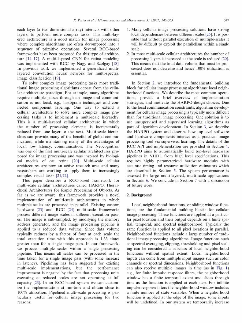
Local neighborhood functions, or sliding window func-tions, are the fundamental building blocks for cellularimage processing. These functions are applied at a particu-lar pixel location and their output depends on a finite spa-tial, temporal, and spectral neighborhood. Typically thesame function is applied to all pixel locations in parallel.Neighborhood functions include a large number of tradi-tional image processing algorithms. Image functions suchas spectral averaging, clipping, thresholding and pixel scal-ing can be considered a subclass of local neighborhoodfunctions without spatial extent. Local neighborhoodinputs can come from multiple input images such as colorchannels or spectral dimensions. Neighborhood functionscan also receive multiple images in time (as in Fig. 1)e.g., for finite impulse response filters, the neighborhoodwindow has a finite temporal extent and slides throughtime as the function is applied at each step. For infiniteimpulse response filters the neighborhood window includesa finite number of state variables. When a neighborhoodfunction is applied at the edge of the image, some inputswill be undefined. In our system we temporarily increase

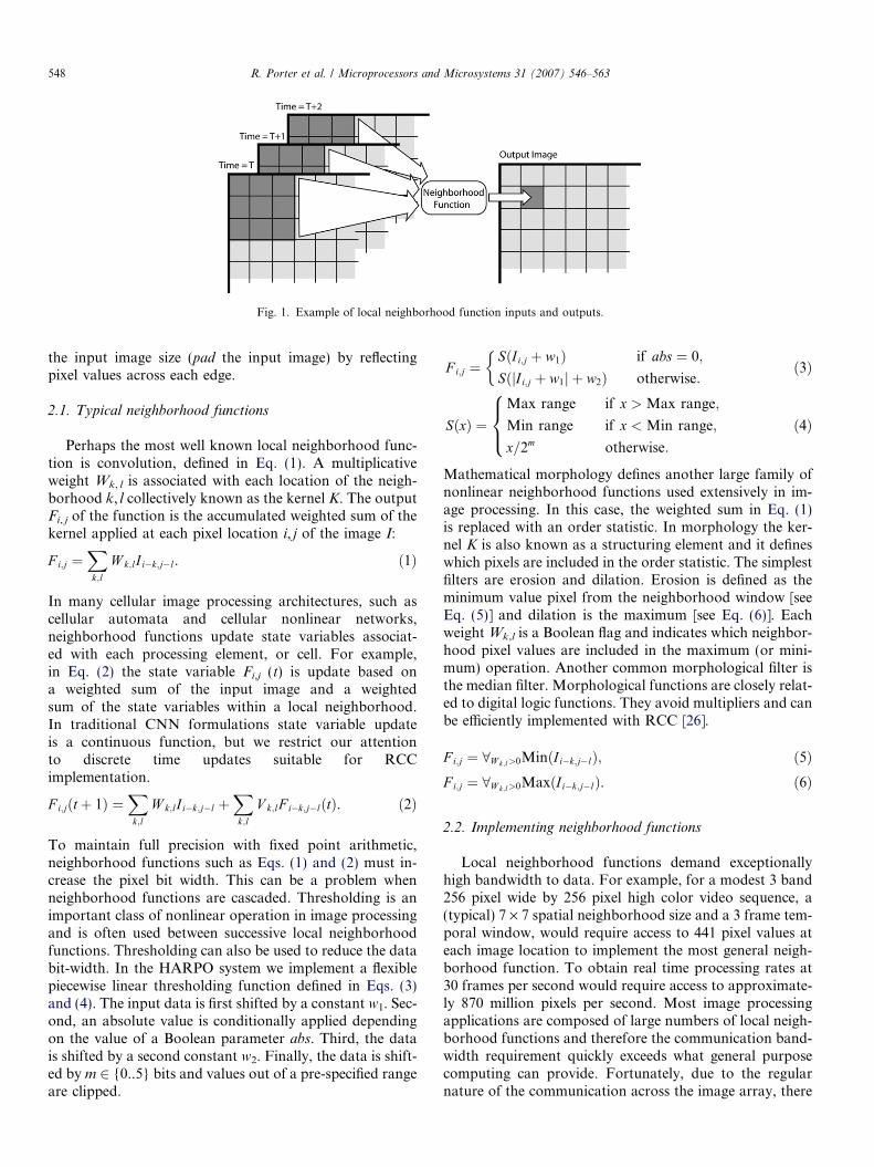
Fig. 1. Example of local neighborhood function inputs and outputs.

548 R. Porter et al. / Microprocessors and Microsystems 31 (2007) 546–563

the input image size (pad the input image) by reflectingpixel values across each edge.

2.1. Typical neighborhood functions

Perhaps the most well known local neighborhood func-tion is convolution, defined in Eq. (1). A multiplicativeweight Wk, l is associated with each location of the neigh-borhood k, l collectively known as the kernel K. The outputFi, j of the function is the accumulated weighted sum of thekernel applied at each pixel location i, j of the image I:

F i;j ¼X

k;l

W k;lI i�k;j�l. ð1Þ

In many cellular image processing architectures, such ascellular automata and cellular nonlinear networks,neighborhood functions update state variables associat-ed with each processing element, or cell. For example,in Eq. (2) the state variable Fi,j (t) is update based ona weighted sum of the input image and a weightedsum of the state variables within a local neighborhood.In traditional CNN formulations state variable updateis a continuous function, but we restrict our attentionto discrete time updates suitable for RCCimplementation.

F i;jðtþ 1Þ ¼X

k;l

W k;lI i�k;j�l þX

k;l

V k;lF i�k;j�lðtÞ. ð2Þ

To maintain full precision with fixed point arithmetic,neighborhood functions such as Eqs. (1) and (2) must in-crease the pixel bit width. This can be a problem whenneighborhood functions are cascaded. Thresholding is animportant class of nonlinear operation in image processingand is often used between successive local neighborhoodfunctions. Thresholding can also be used to reduce the databit-width. In the HARPO system we implement a flexiblepiecewise linear thresholding function defined in Eqs. (3)and (4). The input data is first shifted by a constant w1. Sec-ond, an absolute value is conditionally applied dependingon the value of a Boolean parameter abs. Third, the datais shifted by a second constant w2. Finally, the data is shift-ed by m 2 {0..5} bits and values out of a pre-specified rangeare clipped.

F i;j ¼SðI i;j þ w1Þ if abs ¼ 0;

SðjI i;j þ w1j þ w2Þ otherwise:

�ð3Þ

SðxÞ ¼Max range if x > Max range;

Min range if x < Min range;

x=2m otherwise:

8><>: ð4Þ

Mathematical morphology defines another large family ofnonlinear neighborhood functions used extensively in im-age processing. In this case, the weighted sum in Eq. (1)is replaced with an order statistic. In morphology the ker-nel K is also known as a structuring element and it defineswhich pixels are included in the order statistic. The simplestfilters are erosion and dilation. Erosion is defined as theminimum value pixel from the neighborhood window [seeEq. (5)] and dilation is the maximum [see Eq. (6)]. Eachweight Wk,l is a Boolean flag and indicates which neighbor-hood pixel values are included in the maximum (or mini-mum) operation. Another common morphological filter isthe median filter. Morphological functions are closely relat-ed to digital logic functions. They avoid multipliers and canbe efficiently implemented with RCC [26].

F i;j ¼ 8W k;l>0MinðI i�k;j�lÞ; ð5ÞF i;j ¼ 8W k;l>0MaxðI i�k;j�lÞ. ð6Þ

2.2. Implementing neighborhood functions

Local neighborhood functions demand exceptionallyhigh bandwidth to data. For example, for a modest 3 band256 pixel wide by 256 pixel high color video sequence, a(typical) 7 · 7 spatial neighborhood size and a 3 frame tem-poral window, would require access to 441 pixel values ateach image location to implement the most general neigh-borhood function. To obtain real time processing rates at30 frames per second would require access to approximate-ly 870 million pixels per second. Most image processingapplications are composed of large numbers of local neigh-borhood functions and therefore the communication band-width requirement quickly exceeds what general purposecomputing can provide. Fortunately, due to the regularnature of the communication across the image array, there


are also many opportunities to optimize the bandwidth.Reconfigurable computers are ideal platforms to tailorhigh-bandwidth memory hierarchies and implement algo-rithm specific address generation. There are two main waysthat local neighborhood functions are implemented:

2.2.1. Data parallel

Many implementations exploit the parallel nature of cel-lular array directly by implementing a large number of pro-cessing elements, each associated with a specific pixellocation. At the extreme of this approach all pixels are pro-cessed in parallel, each cell has direct access to neighboringpixels at all times, and the entire array is updated in 1 clockcycle. This implementation is illustrated on the left inFig. 2. RCC can implement a programmable, maximallyparallel implementation of a cellular array, but can onlyefficiently implement a small numbers of cells. Large arraysrequire time multiplexing, and the time taken to initializethe array and communicate results is typically much largerthan the computation time.

2.2.2. Instruction parallelWhen implementing synchronous systems (as we are in

RCC) it is also possible to achieve parallelism via pipelin-ing. At the extreme of this approach only one cell is imple-mented for an entire array and each pixel location withinthe array is updated sequentially. The output stream fromthe first array is then directly tied to the input stream of asecond array and therefore a long chain of instructions canbe executed each clock cycle. Each instruction must accessits local neighborhood at the same time and thereforeimage data must be cached within the computing devicein large shift registers. This implementation is illustratedon the right in Fig. 2.

We have described the two extremes of a pixel parallelversus instruction parallel design space. In practice anycombination of these two extremes can be used. The opti-mal design point is dictated largely by the memory band-width that is available both on-chip and off-chip. Mostmodern FPGA devices now offer large quantities of on-chip memory which is ideal for implementing the large shift

Fig. 2. Data versus in

registers required in pipelining. By exploiting internalmemory bandwidth, an instruction parallel design placesless demand on external memory bandwidth (only 1 pix-el/clock cycle is required). The instruction parallelapproach has some inefficiency due to pipeline latencyand edge conditions. For an image W pixels high by W pix-els wide, each instruction introduces a aW latency, where ais proportional to the local neighborhood size. Also, foreach neighborhood instruction the valid output image isreduced in size by a pixels due to edge conditions. For P

pipelined instructions this means approximately PaW pixelcalculations are invalid.

The total execution time for the pipeline is W2 andtherefore for practical image sizes, W � 1000, the impacton performance is usually not significant.

The HARPO framework adopts the instruction parallelapproach at the extreme and reads one pixel location frommemory each clock cycle. This read includes multiple pix-els, but each pixel comes from a different input image.The main motivation for this approach is to accelerateextremely large networks where the external bandwidthwould be completely utilized by a large number of inputimages. Depending on the application, this design choicemay not be optimal and external bandwidth and computa-tional resources may go unused. In this case it would be rel-atively straight-forward to generalize the HARPO systemto include data parallel pipelines.

3. System overview

An overview of the HARPO system is shown in Fig. 3.HARPO operates in two modes: run-time mode and

training mode. In the run-time mode HARPO is appliedas an online system. Video frames are loaded sequentiallyand passed to the system one at a time. After a fixed num-ber of frames latency (the latency depends on the applica-tion) HARPO will start producing an output videostream. The output is a video overlay where high pixel val-ues indicate objects or features of interest, e.g., particularvehicles, land cover, etc. HARPO can also produce addi-tional meta-data such as predicted locations, percentage

struction parallel.

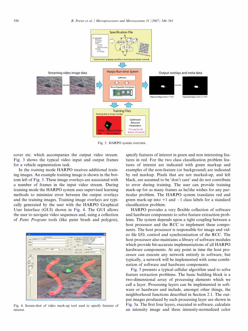
Fig. 3. HARPO system overview.


cover etc. which accompanies the output video stream.Fig. 3 shows the typical video input and output framesfor a vehicle segmentation task.

In the training mode HARPO receives additional train-ing images. An example training image is shown in the bot-tom left of Fig. 3. These image overlays are associated witha number of frames in the input video stream. Duringtraining mode the HARPO system uses supervised learningmethods to minimize error between the output overlaysand the training images. Training image overlays are typi-cally generated by the user with the HARPO GraphicalUser Interface (GUI) shown in Fig. 4. The GUI allowsthe user to navigate video sequences and, using a collectionof Paint Program tools (like paint brush and polygon),

Fig. 4. Screen-shot of video mark-up tool used to specify features ofinterest.

specify features of interest in green and non interesting fea-tures in red. For the two class classification problem fea-tures of interest are indicated with green markup andexamples of the non-feature (or background) are indicatedby red markup. Pixels that are not marked-up, and leftblack, are assumed to be ‘don’t care’ and do not contributeto error during training. The user can provide trainingmark-up for as many frames as he/she wishes for any par-ticular problem. The HARPO system translates red andgreen mark-up into +1 and �1 class labels for a standardclassification problem.

HARPO provides a very flexible collection of softwareand hardware components to solve feature extraction prob-lems. The system depends upon a tight coupling between ahost processor and the RCC to implement these compo-nents. The host processor is responsible for image and vid-eo file I/O, control and synchronization of the RCC. Thehost processor also maintains a library of software moduleswhich provide bit-accurate implementations of all HARPOhardware components. At any point in time the host pro-cessor can execute any network entirely in software, buttypically, a network will be implemented with some combi-nation of software and hardware components.

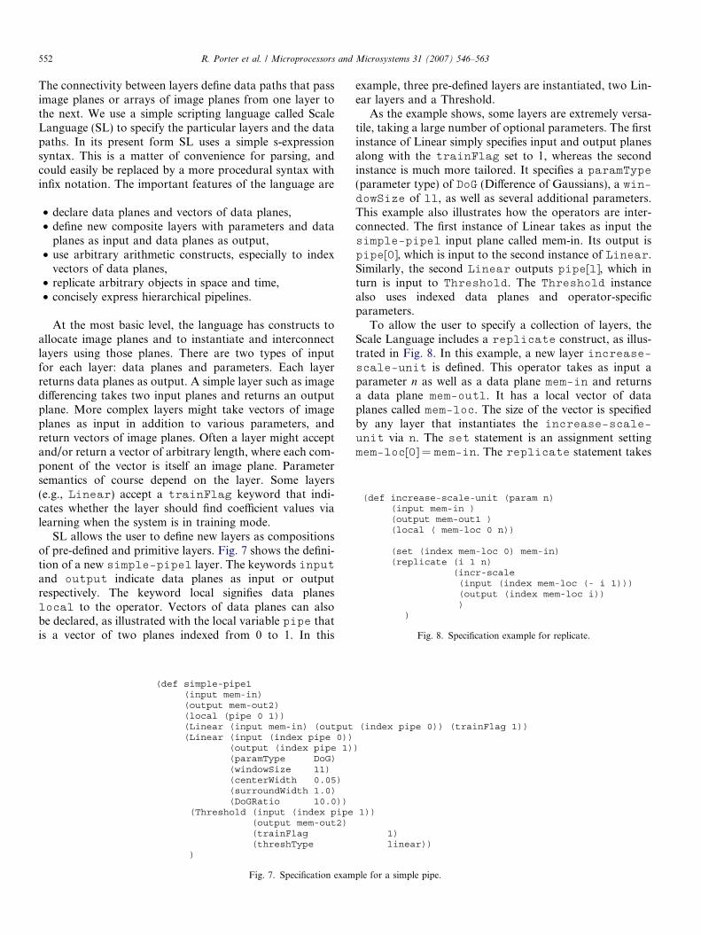
Fig. 5 presents a typical cellular algorithm used to solvefeature extraction problems. The basic building block is atwo-dimensional array of processing elements which wecall a layer. Processing layers can be implemented in soft-ware or hardware and include, amongst other things, theneighborhood functions described in Section 2.1. The out-put images produced by each processing layer are shown inFig. 5a. The first four layers, executed in software, calculatean intensity image and three intensity-normalized color

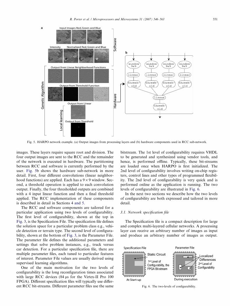
Fig. 5. HARPO network example. (a) Output images from processing layers and (b) hardware components used in RCC sub-network.

Fig. 6. The two-levels of configurability.


images. These layers require square root and division. Thefour output images are sent to the RCC and the remainderof the network is executed in hardware. The partitioningbetween RCC and software is currently performed by theuser. Fig. 5b shows the hardware sub-network in moredetail. First, four different convolutions (linear neighbor-hood functions) are applied. Each has a 9 · 9 window. Sec-ond, a threshold operation is applied to each convolutionoutput. Finally, the four thresholded outputs are combinedwith a 4 input linear function and then a final thresholdapplied. The RCC implementation of these componentsis described in detail in Sections 4 and 5.

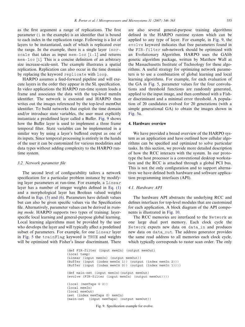
The RCC and software components are tailored for aparticular application using two levels of configurability.The first level of configurability, shown at the top inFig. 3, is the Specification File. The specification file definesthe solution space for a particular problem class e.g., vehi-cle detection or terrain type. The second level of configura-bility, shown at the bottom of Fig. 3, is the Parameter File.The parameter file defines the additional parameters andsettings that solve problem instances, e.g., truck versuscar detection. For a particular specification file, there aremultiple parameter files, each tuned to particular featuresof interest. Parameter File values are usually derived usingsupervised learning algorithms.

One of the main motivation for the two levels ofconfigurability is the long reconfiguration times associatedwith large RCC devices (84 ls for the Virtex-II Pro 100FPGA). Different specification files will typically use differ-ent RCC bit-streams. Different parameter files use the same

bitstream. The 1st level of configurability requires VHDLto be generated and synthesized using vendor tools, andhence, is performed offline. Typically, these bit-streamsare loaded once when HARPO is first initialized. The2nd level of configurability involves writing on-chip regis-ters, control lines and other types of programmed flexibil-ity. The 2nd level of configurability is very quick and isperformed online as the application is running. The twolevels of configurability are illustrated in Fig. 6.

In the next two sections we describe how the two levelsof configurability are both expressed and tailored in moredetail.

3.1. Network specification file

The Specification file is a compact description for largeand complex multi-layered cellular networks. A processinglayer can receive an arbitrary number of images as inputand produce an arbitrary number of images as output.

(def increase-scale-unit (param n) (input mem-in ) (output mem-out1 ) (local ( mem-loc 0 n)) (set (index mem-loc 0) mem-in) (replicate (i 1 n) (incr-scale (input (index mem-loc (- i 1))) (output (index mem-loc i)) )

)

Fig. 8. Specification example for replicate.


The connectivity between layers define data paths that passimage planes or arrays of image planes from one layer tothe next. We use a simple scripting language called ScaleLanguage (SL) to specify the particular layers and the datapaths. In its present form SL uses a simple s-expressionsyntax. This is a matter of convenience for parsing, andcould easily be replaced by a more procedural syntax withinfix notation. The important features of the language are

• declare data planes and vectors of data planes,• define new composite layers with parameters and data

planes as input and data planes as output,• use arbitrary arithmetic constructs, especially to index

vectors of data planes,• replicate arbitrary objects in space and time,• concisely express hierarchical pipelines.

At the most basic level, the language has constructs toallocate image planes and to instantiate and interconnectlayers using those planes. There are two types of inputfor each layer: data planes and parameters. Each layerreturns data planes as output. A simple layer such as imagedifferencing takes two input planes and returns an outputplane. More complex layers might take vectors of imageplanes as input in addition to various parameters, andreturn vectors of image planes. Often a layer might acceptand/or return a vector of arbitrary length, where each com-ponent of the vector is itself an image plane. Parametersemantics of course depend on the layer. Some layers(e.g., Linear) accept a trainFlag keyword that indi-cates whether the layer should find coefficient values vialearning when the system is in training mode.

SL allows the user to define new layers as compositionsof pre-defined and primitive layers. Fig. 7 shows the defini-tion of a new simple-pipe1 layer. The keywords inputand output indicate data planes as input or outputrespectively. The keyword local signifies data planeslocal to the operator. Vectors of data planes can alsobe declared, as illustrated with the local variable pipe thatis a vector of two planes indexed from 0 to 1. In this

(def simple-pipe1 (input mem-in) (output mem-out2) (local (pipe 0 1)) (Linear (input mem-in) (output (Linear (input (index pipe 0)) (output (index pipe 1) (paramType DoG) (windowSize 11) (centerWidth 0.05) (surroundWidth 1.0) (DoGRatio 10.0)) (Threshold (input (index pipe (output mem-out2) (trainFlag (threshType )

Fig. 7. Specification exam

example, three pre-defined layers are instantiated, two Lin-ear layers and a Threshold.

As the example shows, some layers are extremely versa-tile, taking a large number of optional parameters. The firstinstance of Linear simply specifies input and output planesalong with the trainFlag set to 1, whereas the secondinstance is much more tailored. It specifies a paramType

(parameter type) of DoG (Difference of Gaussians), a win-dowSize of 11, as well as several additional parameters.This example also illustrates how the operators are inter-connected. The first instance of Linear takes as input thesimple-pipe1 input plane called mem-in. Its output ispipe[0], which is input to the second instance of Linear.Similarly, the second Linear outputs pipe[1], which inturn is input to Threshold. The Threshold instancealso uses indexed data planes and operator-specificparameters.

To allow the user to specify a collection of layers, theScale Language includes a replicate construct, as illus-trated in Fig. 8. In this example, a new layer increase-scale-unit is defined. This operator takes as input aparameter n as well as a data plane mem-in and returnsa data plane mem-out1. It has a local vector of dataplanes called mem-loc. The size of the vector is specifiedby any layer that instantiates the increase-scale-

unit via n. The set statement is an assignment settingmem-loc[0] = mem-in. The replicate statement takes

(index pipe 0)) (trainFlag 1)) )

1))

1) linear))

ple for a simple pipe.


as the first argument a range of replications. The firstparameter (i in the example) is an identifier that is boundto each index in the replication range. Following is a list oflayers to be instantiated, each of which is replicated overthe range. In the example, there is a single layer incr-

scale that takes as input mem-loc [i-1] and returnsmem-loc [i]. This is a concise definition of an arbitrarysize increase-scale-unit. The example illustrates a spatialreplication. Replication can also occur in the time domainby replacing the keyword replicate with loop.

HARPO assumes a feed-forward pipeline and will exe-cute layers in the order they appear in the SL specification.In video applications the HARPO run-time system loads aframe and associates the data with the top-level memInidentifier. The network is executed and HARPO thenwrites out the images referenced by the top-level memOutidentifier. To build networks that exploit the time domainand/or introduce state variables, the user must explicitlyinstantiate a predefined layer called a Buffer. Fig. 9 showshow the Buffer layer is used to implement a three frametemporal filter. State variables can be implemented in asimilar way by using a layer’s buffered output as one ofits inputs. Since temporal processing is entirely in the handsof the user it can be customized for various modalities anddata types without adding complexity to the HARPO run-time system.

3.2. Network parameter file

The second level of configurability tailors a networkspecification for a particular problem instance by modify-ing layer parameters at run-time. For example, a Linear

layer has a number of integer weights defined in Eq. (1)and a morphological layer has Boolean valued weightsdefined in Eqs. (5) and (6). Parameters have default valuesbut can also be given specific values via the Specificationfile. Alternatively, parameter values can be derived in train-

ing mode. HARPO supports two types of training: layer-specific local learning and general-purpose global learning.Local learning algorithms must be provided by the userwho develops the layer and will typically affect a predefinedsubset of parameters. For example, for one Linear layerin Fig. 5 the trainFlag keyword is TRUE and weightswill be optimized with Fisher’s linear discriminant. There

(def FIR-filter (input memIn) ((local temp) (Linear (input memIn) (output m(Buffer (input (index memIn 1))(Buffer (input (index memIn 0))

(def main-net (input memIn)(out(evolve (FIR-filter (input memI

(local (memTaps 0 2)) (local memIn) (local memOut) (set (index memTaps 0) memIn) (main-net (input memTaps) (out

Fig. 9. Specification ex

are also several general-purpose training algorithmsdefined in the HARPO runtime system which can beapplied to any type of layer. For example, in Fig. 9, theevolve keyword indicates that free parameters found inthe FIR-filter sub-network should be optimized withan Evolutionary Algorithm. HARPO uses the GAlibgenetic algorithm package, written by Matthew Wall atthe Massachusetts Institute of Technology for these algo-rithms. A useful strategy for optimizing network parame-ters is to use a combination of global learning and locallearning algorithms. For example, for each evaluation ofthe GA in Fig. 5, parameter values for the four convolu-tions and threshold functions are randomly generated,applied to the input image, and then combined with a Fish-er discriminant and a minimal error threshold. A popula-tion of 20 candidates evolved for 20 generations (with asimple generational GA) to obtain the images shown inFig. 5a.

4. Hardware overview

We have provided a broad overview of the HARPO sys-tem as an application and have outlined how cellular algo-rithms can be specified and optimized to solve particulartasks. In this section, we provide more detailed descriptionof how the RCC interacts with the system. In our proto-type the host processor is a conventional desktop worksta-tion and the RCC is attached through a global PCI bus.This is not the only configuration and to support alterna-tives we have defined both hardware and software applica-tion programming interfaces (API).

4.1. Hardware API

The hardware API abstracts the underlying RCC anddefines interfaces for top-level modules that are customizedfor each application. A block diagram of the API compo-nents is illustrated in Fig. 10.

The RCC memories are interfaced to the Network asone large dual port memory. Each clock cycle theNetwork expects new data on data_in and producesnew data on data_out. The address generator providesthe same read address to all memories each clock cycle,which typically corresponds to raster scan order. The only

output memOut)

emOut)) (output (index memIn 2))) (output (index memIn 1))))

put memOut) n) (output memOut))))

put memOut))

ample for evolve.

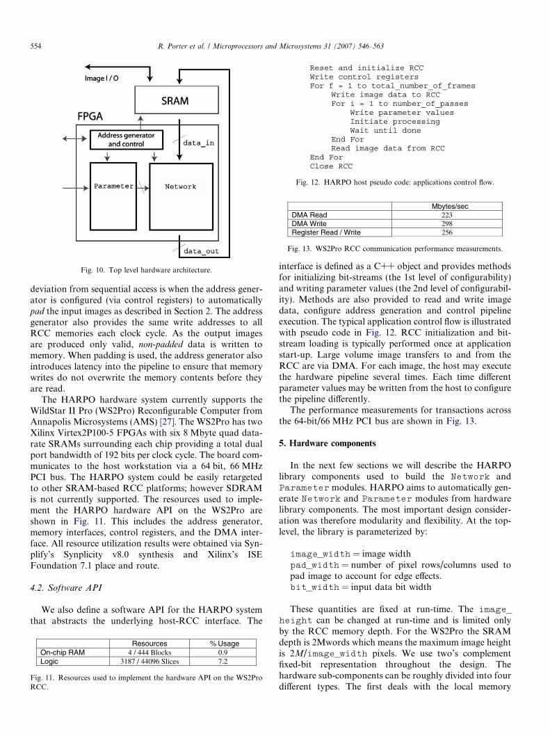
Reset and initialize RCC Write control registers For f = 1 to total_number_of_frames Write image data to RCC For i = 1 to number_of_passes

Write parameter values Initiate processing Wait until done

End For Read image data from RCC

End For Close RCC

Fig. 12. HARPO host pseudo code: applications control flow.

Mbytes/sec DMA Read 223 DMA Write 298 Register Read / Write 256

Fig. 13. WS2Pro RCC communication performance measurements.

Fig. 10. Top level hardware architecture.


deviation from sequential access is when the address gener-ator is configured (via control registers) to automaticallypad the input images as described in Section 2. The addressgenerator also provides the same write addresses to allRCC memories each clock cycle. As the output imagesare produced only valid, non-padded data is written tomemory. When padding is used, the address generator alsointroduces latency into the pipeline to ensure that memorywrites do not overwrite the memory contents before theyare read.

The HARPO hardware system currently supports theWildStar II Pro (WS2Pro) Reconfigurable Computer fromAnnapolis Microsystems (AMS) [27]. The WS2Pro has twoXilinx Virtex2P100-5 FPGAs with six 8 Mbyte quad data-rate SRAMs surrounding each chip providing a total dualport bandwidth of 192 bits per clock cycle. The board com-municates to the host workstation via a 64 bit, 66 MHzPCI bus. The HARPO system could be easily retargetedto other SRAM-based RCC platforms; however SDRAMis not currently supported. The resources used to imple-ment the HARPO hardware API on the WS2Pro areshown in Fig. 11. This includes the address generator,memory interfaces, control registers, and the DMA inter-face. All resource utilization results were obtained via Syn-plify’s Synplicity v8.0 synthesis and Xilinx’s ISEFoundation 7.1 place and route.

4.2. Software API

We also define a software API for the HARPO systemthat abstracts the underlying host-RCC interface. The

Resources % UsageOn-chip RAM 4 / 444 Blocks 0.9 Logic 3187 / 44096 Slices 7.2

Fig. 11. Resources used to implement the hardware API on the WS2ProRCC.

interface is defined as a C++ object and provides methodsfor initializing bit-streams (the 1st level of configurability)and writing parameter values (the 2nd level of configurabil-ity). Methods are also provided to read and write imagedata, configure address generation and control pipelineexecution. The typical application control flow is illustratedwith pseudo code in Fig. 12. RCC initialization and bit-stream loading is typically performed once at applicationstart-up. Large volume image transfers to and from theRCC are via DMA. For each image, the host may executethe hardware pipeline several times. Each time differentparameter values may be written from the host to configurethe pipeline differently.

The performance measurements for transactions acrossthe 64-bit/66 MHz PCI bus are shown in Fig. 13.

5. Hardware components

In the next few sections we will describe the HARPOlibrary components used to build the Network andParameter modules. HARPO aims to automatically gen-erate Network and Parameter modules from hardwarelibrary components. The most important design consider-ation was therefore modularity and flexibility. At the top-level, the library is parameterized by:

image_width = image widthpad_width = number of pixel rows/columns used topad image to account for edge effects.bit_width = input data bit width

These quantities are fixed at run-time. The image_height can be changed at run-time and is limited onlyby the RCC memory depth. For the WS2Pro the SRAMdepth is 2Mwords which means the maximum image heightis 2M/image_width pixels. We use two’s complementfixed-bit representation throughout the design. Thehardware sub-components can be roughly divided into fourdifferent types. The first deals with the local memory


management required by neighborhood functions. We havedeveloped a versatile and programmable window modulewhich can be instantiated and used for any local neighbor-hood function at any scale. This module is described in Sec-tion 5.1. The second type of component includes specificneighborhood functions, such as convolution and isdescribed in Section 5.2. The third type of component,described in Section 5.3, is used for data sequencing andincludes down sampling and up sampling. The fourth com-ponent is used in the Parameter module and provides theinterface between the Network module and the host pro-cessor to provide run-time configurability.

5.1. Neighborhood memory access

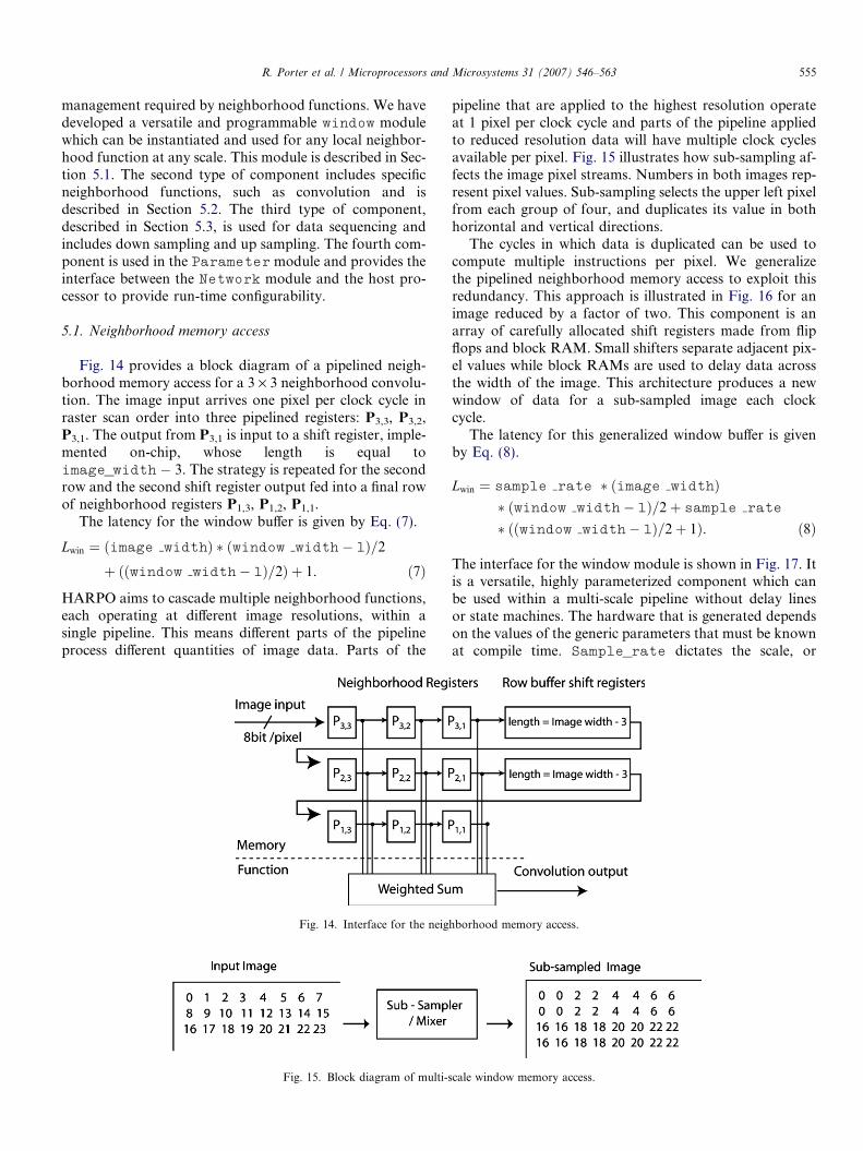
Fig. 14 provides a block diagram of a pipelined neigh-borhood memory access for a 3 · 3 neighborhood convolu-tion. The image input arrives one pixel per clock cycle inraster scan order into three pipelined registers: P3,3, P3,2,P3,1. The output from P3,1 is input to a shift register, imple-mented on-chip, whose length is equal toimage_width � 3. The strategy is repeated for the secondrow and the second shift register output fed into a final rowof neighborhood registers P1,3, P1,2, P1,1.

The latency for the window buffer is given by Eq. (7).

Lwin ¼ ðimage widthÞ � ðwindow width� 1Þ=2

þ ððwindow width� 1Þ=2Þ þ 1. ð7Þ

HARPO aims to cascade multiple neighborhood functions,each operating at different image resolutions, within asingle pipeline. This means different parts of the pipelineprocess different quantities of image data. Parts of the

Fig. 14. Interface for the neig

Fig. 15. Block diagram of multi-s

pipeline that are applied to the highest resolution operateat 1 pixel per clock cycle and parts of the pipeline appliedto reduced resolution data will have multiple clock cyclesavailable per pixel. Fig. 15 illustrates how sub-sampling af-fects the image pixel streams. Numbers in both images rep-resent pixel values. Sub-sampling selects the upper left pixelfrom each group of four, and duplicates its value in bothhorizontal and vertical directions.

The cycles in which data is duplicated can be used tocompute multiple instructions per pixel. We generalizethe pipelined neighborhood memory access to exploit thisredundancy. This approach is illustrated in Fig. 16 for animage reduced by a factor of two. This component is anarray of carefully allocated shift registers made from flipflops and block RAM. Small shifters separate adjacent pix-el values while block RAMs are used to delay data acrossthe width of the image. This architecture produces a newwindow of data for a sub-sampled image each clockcycle.

The latency for this generalized window buffer is givenby Eq. (8).

Lwin ¼ sample rate � ðimage widthÞ� ðwindow width� 1Þ=2þ sample rate

� ððwindow width� 1Þ=2þ 1Þ. ð8Þ

The interface for the window module is shown in Fig. 17. Itis a versatile, highly parameterized component which canbe used within a multi-scale pipeline without delay linesor state machines. The hardware that is generated dependson the values of the generic parameters that must be knownat compile time. Sample_rate dictates the scale, or

hborhood memory access.

cale window memory access.

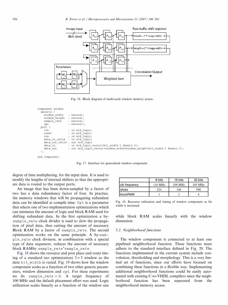
8 bits 16 bits 32 bits

clk frequency 116 MHz 109 MHz 105 MHz

slices 224 346 590

blockRAM 1 2 4

Fig. 18. Resource utilization and timing of window component as bitwidth is increased.

Fig. 16. Block diagram of multi-scale window memory access.

component window generic ( window_width : natural; window_height : natural; sample_rate : natural; opt : natural); port ( clk : in std_logic; reset : in std_logic; run : in std_logic; data_in_valid : in std_logic; data_out_valid : out std_logic data_in : in std_logic_vector(bit_width-1 downto 0); data_out : out std_logic_vector(window_width*window_height*bit_width-1 downto 0); );

end component;

Fig. 17. Interface for generalized window component.


degree of time multiplexing, for the input data. It is used tomodify the lengths of internal shifters so that the appropri-ate data is routed to the output ports.

An image that has been down-sampled by a factor oftwo has a data redundancy factor of four. In practice,the memory windows that will be propagating redundantdata can be identified at compile time. Opt is a parameterthat selects one of two implementation optimizations whichcan minimize the amount of logic and block RAM used forshifting redundant data. In the first optimization a by-sample_rate clock divider is used to slow the propaga-tion of pixel data, thus cutting the amount of necessaryBlock RAM by a factor of sample_rate. The secondoptimization works on the same principle. A by-sam-ple_rate clock division, in combination with a specialtype of data sequencer, reduces the amount of necessaryblock RAMby sample_rate*sample_rate.

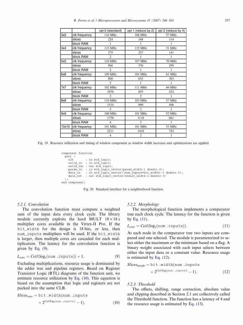
Fig. 18 shows the resource and post place and route tim-ing of a standard (no optimization) 3 · 3 window as thedata bit_width is varied. Fig. 19 shows how the windowcomponent scales as a function of two other generic param-eters, window dimension and opt. For these experimentswe fix sample_rate = 2. A target frequency of100 MHz and the default placement effort was used. Logicutilization scales linearly as a function of the window size

while block RAM scales linearly with the windowdimension.

5.2. Neighborhood functions

The window component is connected to at least onepipelined neighborhood function. These functions mustadhere to the standard interface defined in Fig. 20. Thefunctions implemented in the current system include con-volution, thresholding and morphology. This is a very lim-ited set of functions, since our efforts have focused oncombining these functions in a flexible way. Implementingadditional neighborhood functions could be easily auto-mated with existing C-to-VHDL compilers since the neigh-borhood function has been separated from theneighborhood memory access.

opt 0 (standard) opt 1 (reduce by 2) opt 2 (reduce by 4)3x3 clk frequency 116 MHz 106 MHz 57 MHz

slices 224 168 114block RAM 1 1 1

4x4 clk frequency 123 MHz 125 MHz 51 MHzslices 375 257 141block RAM 2 1 1







Fig. 19. Resource utilization and timing of window component as window width increases and optimizations are applied.

component function port ( clk : in std_logic; valid_in : in std_logic; valid_out : out std_logic; param_in : in std_logic_vector(param_width-1 downto 0); data_in : in std_logic_vector((num_inputs*bit_width)-1 downto 0); data_out : out std_logic_vector(result_width-1 downto 0) ); end component;

Fig. 20. Standard interface for a neighborhood function.


5.2.1. Convolution

The convolution function must compute a weightedsum of the input data every clock cycle. The librarymodule currently exploits the hard MULT 18 · 18 smultiplier cores available in the Virtex-II Pro. If thebit_width for the design is 18 bits, or less, thennum_inputs multipliers will be used. If the bit_widthis larger, then multiple cores are cascaded for each mul-tiplication. The latency for the convolution function isgiven by Eq. (9).

Lconv ¼ Ceilðlog2ðnum inputsÞÞ þ 1. ð9ÞExcluding multiplications, resource usage is dominated bythe adder tree and pipeline registers. Based on RegisterTransistor Logic (RTL) diagrams of the function unit, weestimate resource utilization by Eq. (10). This equation isbased on the assumption that logic and registers are notpacked into the same CLB.

Slicesconv ¼ bit widthðnum inputs

þ 2Ceilðlog2ðnum inputsÞÞ � 1Þ. ð10Þ

5.2.2. Morphology

The morphological function implements a comparatortree each clock cycle. The latency for the function is givenby Eq. (11).

Lconv ¼ Ceilðlog2ðnum inputsÞÞ. ð11ÞAt each node in the comparator tree two inputs are com-pared and one selected. The module is parameterized to se-lect either the maximum or the minimum based on a flag. Abinary weight associated with each input selects betweeneither the input data or a constant value. Resource usageis estimated by Eq. (12).

Slicesmorph ¼ bit widthðnum inputs

þ 2Ceilðlog2ðnum inputsÞÞ � 1Þ. ð12Þ

5.2.3. Threshold

The offsets, shifting, range correction, absolute valueand clipping described in Section 2.1 are collectively calledthe Threshold function. The function has a latency of 4 andthe resource usage is estimated by Eq. (13).


Slicesthresh ¼ 12:bit width . ð13Þ

5.3. Data sequencing

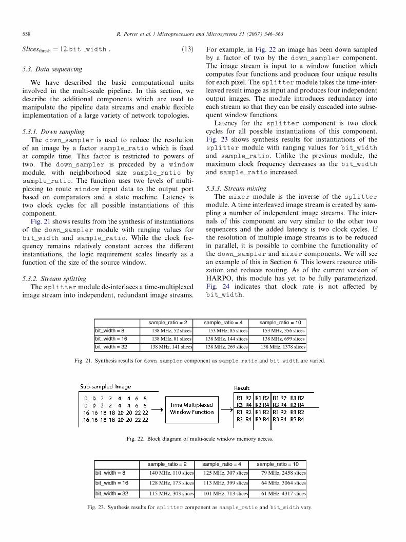
We have described the basic computational unitsinvolved in the multi-scale pipeline. In this section, wedescribe the additional components which are used tomanipulate the pipeline data streams and enable flexibleimplementation of a large variety of network topologies.

5.3.1. Down sampling

The down_sampler is used to reduce the resolutionof an image by a factor sample_ratio which is fixedat compile time. This factor is restricted to powers oftwo. The down_sampler is preceded by a window

module, with neighborhood size sample_ratio bysample_ratio. The function uses two levels of multi-plexing to route window input data to the output portbased on comparators and a state machine. Latency istwo clock cycles for all possible instantiations of thiscomponent.

Fig. 21 shows results from the synthesis of instantiationsof the down_sampler module with ranging values forbit_width and sample_ratio. While the clock fre-quency remains relatively constant across the differentinstantiations, the logic requirement scales linearly as afunction of the size of the source window.

5.3.2. Stream splitting

The splitter module de-interlaces a time-multiplexedimage stream into independent, redundant image streams.

sample_ratio = 2 s

bit_width = 8 138 MHz, 52 slices



Fig. 21. Synthesis results for down_sampler compone

Fig. 22. Block diagram of multi-s

sample_ratio = 2 s

bit_width = 8 140 MHz, 110 slices 1



Fig. 23. Synthesis results for splitter compone

For example, in Fig. 22 an image has been down sampledby a factor of two by the down_sampler component.The image stream is input to a window function whichcomputes four functions and produces four unique resultsfor each pixel. The splitter module takes the time-inter-leaved result image as input and produces four independentoutput images. The module introduces redundancy intoeach stream so that they can be easily cascaded into subse-quent window functions.

Latency for the splitter component is two clockcycles for all possible instantiations of this component.Fig. 23 shows synthesis results for instantiations of thesplitter module with ranging values for bit_widthand sample_ratio. Unlike the previous module, themaximum clock frequency decreases as the bit_widthand sample_ratio increased.

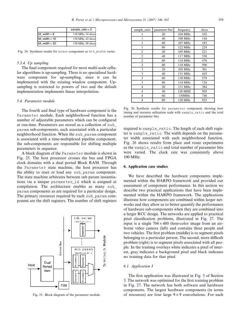
5.3.3. Stream mixing

The mixer module is the inverse of the splitter

module. A time interleaved image stream is created by sam-pling a number of independent image streams. The inter-nals of this component are very similar to the other twosequencers and the added latency is two clock cycles. Ifthe resolution of multiple image streams is to be reducedin parallel, it is possible to combine the functionality ofthe down_sampler and mixer components. We will seean example of this in Section 6. This lowers resource utili-zation and reduces routing. As of the current version ofHARPO, this module has yet to be fully parameterized.Fig. 24 indicates that clock rate is not affected bybit_width.

ample_ratio = 4 sample_ratio = 10

153 MHz, 85 slices 153 MHz, 356 slices



nt as sample_ratio and bit_width are varied.

cale window memory access.

ample_ratio = 4 sample_ratio = 10




nt as sample_ratio and bit_width vary.

sample_ratio parameter bits frequency slices1 20 104 MHz 1031 40 108 MHz 1441 60 107 MHz 1831 80 122 MHz 2242 20 105 MHz 2212 40 117 MHz 3382 60 118 MHz 4782 80 118 MHz 5963 20 105 MHz 3013 40 131 MHz 4453 60 130 MHz 5793 80 134 MHz 7244 20 131 MHz 3844 40 128 MHZ 5654 60 130MHz 7464 80 120 MHz 925

Fig. 26. Synthesis results for parameter component showing howtiming and resource utilization scale with sample_ratio and the totalnumber of parameter bits.

sample_ratio = 2




Fig. 24. Synthesis results for mixer component as bit_width varies.


5.3.4. Up sampling

The final component required for most multi-scale cellu-lar algorithms is up-sampling. There is no specialized hard-ware component for up-sampling, since it can beimplemented with the existing window component. Up-sampling is restricted to powers of two and the defaultimplementation implements linear interpolation.

5.4. Parameter module

The fourth and final type of hardware component is theParameter module. Each neighborhood function has anumber of adjustable parameters which can be configuredat run-time. Parameters are stored as a collection of sub_param sub-components, each associated with a particularneighborhood function. When the sub_param componentis associated with a time-multiplexed pipeline component,the sub-components are responsible for shifting multipleparameters in sequence.

A block diagram of the Parameter module is shown inFig. 25. The host processor crosses the bus and FPGAclock domains with a dual ported Block RAM. Throughthe Parameter state machine, the host processor hasthe ability to reset or load any sub_param component.The state machine arbitrates between sub param instantia-tions via a unique parameter_id which is assigned atcompilation. The architecture enables as many sub_param components as are required for a particular design.The primary resources required by each sub_param com-ponent are the shift registers. The number of shift registers

Fig. 25. Block diagram of the parameter module.

required is sample_ratio. The length of each shift regis-ter is sample_ratio. The width depends on the parame-ter width associated with each neighborhood function.Fig. 26 shows results from place and route experimentsas the sample_ratio and total number of parameter bitswere varied. The clock rate was consistently above100 MHz.

6. Application case studies

We have described the hardware components imple-mented within the HARPO framework and provided ourassessment of component performance. In this section wedescribe two practical applications that have been imple-mented within the HARPO framework. The applicationsillustrate how components are combined within larger net-works and they allow us to better quantify the performanceof hardware sub-components when they are combined intoa larger RCC design. The networks are applied to practicalpixel classification problems, illustrated in Fig. 27. Theinput is a single 704 · 480 three-color image from an air-borne video camera (left) and contains three people andtwo vehicles. The first problem (middle) is to segment pixelsbelonging to a particular person. The second, more difficultproblem (right) is to segment pixels associated with all peo-ple. In the training overlays white indicates a pixel of inter-est, gray indicates a background pixel and black indicatesno training data for that pixel.

6.1. Application I

The first application was illustrated in Fig. 5 of Section3. The network was optimized for the first training problemin Fig. 27. The network has both software and hardwarecomponents. The largest hardware components (in termsof resources) are four large 9 · 9 convolutions. For each

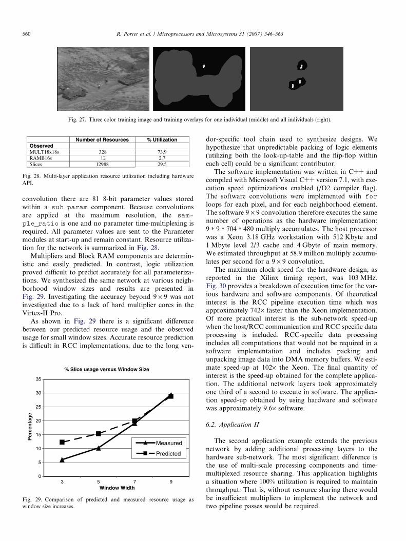
Number of Resources % Utilization Observed MULT18x18s 328 73.9 RAMB16s 2.7 Slices 12988 29.5

12

Fig. 28. Multi-layer application resource utilization including hardwareAPI.

Fig. 27. Three color training image and training overlays for one individual (middle) and all individuals (right).


convolution there are 81 8-bit parameter values storedwithin a sub_param component. Because convolutionsare applied at the maximum resolution, the sam-

ple_ratio is one and no parameter time-multiplexing isrequired. All parameter values are sent to the Parametermodules at start-up and remain constant. Resource utiliza-tion for the network is summarized in Fig. 28.

Multipliers and Block RAM components are determin-istic and easily predicted. In contrast, logic utilizationproved difficult to predict accurately for all parameteriza-tions. We synthesized the same network at various neigh-borhood window sizes and results are presented inFig. 29. Investigating the accuracy beyond 9 · 9 was notinvestigated due to a lack of hard multiplier cores in theVirtex-II Pro.

As shown in Fig. 29 there is a significant differencebetween our predicted resource usage and the observedusage for small window sizes. Accurate resource predictionis difficult in RCC implementations, due to the long ven-

% Slice usage versus Window Size

0

5

10

15

20

25

30

35

3 5 7 9Window Width

Per

cen

tag

e

Measured

Predicted

Fig. 29. Comparison of predicted and measured resource usage aswindow size increases.

dor-specific tool chain used to synthesize designs. Wehypothesize that unpredictable packing of logic elements(utilizing both the look-up-table and the flip-flop withineach cell) could be a significant contributor.

The software implementation was written in C++ andcompiled with Microsoft Visual C++ version 7.1, with exe-cution speed optimizations enabled (/O2 compiler flag).The software convolutions were implemented with for

loops for each pixel, and for each neighborhood element.The software 9 · 9 convolution therefore executes the samenumber of operations as the hardware implementation:9 * 9 * 704 * 480 multiply accumulates. The host processorwas a Xeon 3.18 GHz workstation with 512 Kbyte and1 Mbyte level 2/3 cache and 4 Gbyte of main memory.We estimated throughput at 58.9 million multiply accumu-lates per second for a 9 · 9 convolution.

The maximum clock speed for the hardware design, asreported in the Xilinx timing report, was 103 MHz.Fig. 30 provides a breakdown of execution time for the var-ious hardware and software components. Of theoreticalinterest is the RCC pipeline execution time which wasapproximately 742· faster than the Xeon implementation.Of more practical interest is the sub-network speed-upwhen the host/RCC communication and RCC specific dataprocessing is included. RCC-specific data processingincludes all computations that would not be required in asoftware implementation and includes packing andunpacking image data into DMA memory buffers. We esti-mate speed-up at 102· the Xeon. The final quantity ofinterest is the speed-up obtained for the complete applica-tion. The additional network layers took approximatelyone third of a second to execute in software. The applica-tion speed-up obtained by using hardware and softwarewas approximately 9.6· software.

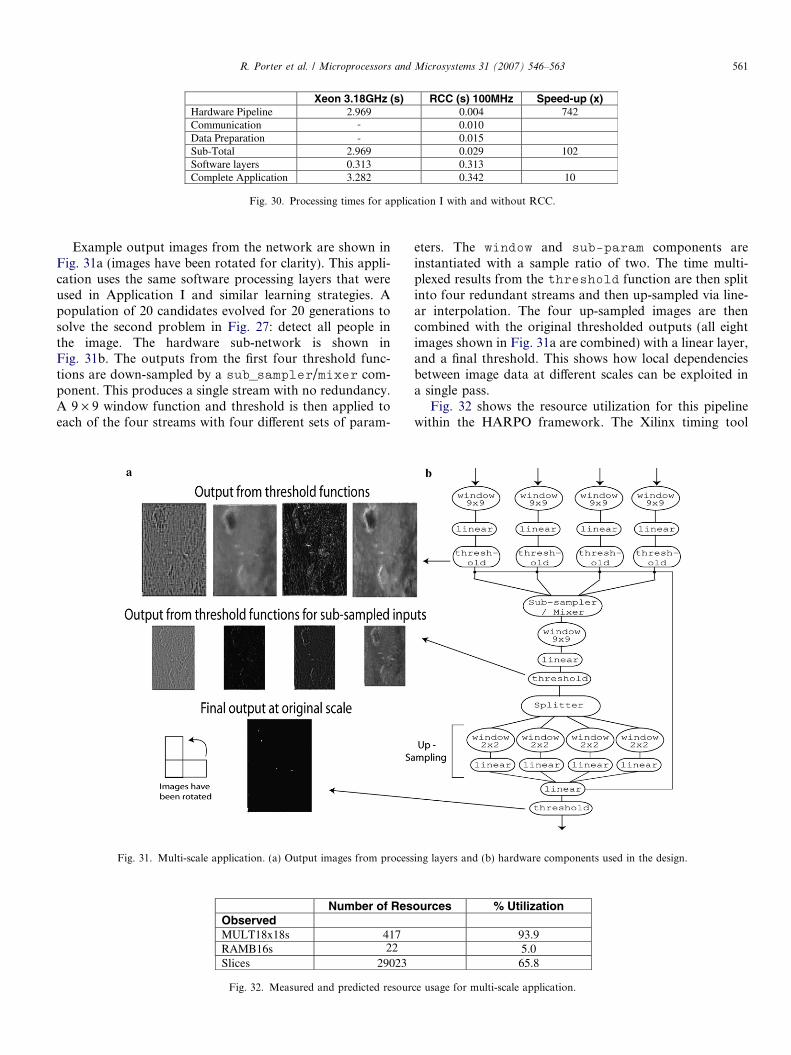
6.2. Application II

The second application example extends the previousnetwork by adding additional processing layers to thehardware sub-network. The most significant difference isthe use of multi-scale processing components and time-multiplexed resource sharing. This application highlightsa situation where 100% utilization is required to maintainthroughput. That is, without resource sharing there wouldbe insufficient multipliers to implement the network andtwo pipeline passes would be required.

Xeon 3.18GHz (s) RCC (s) 100MHz Speed-up (x)Hardware Pipeline 2.969 0.004 742 Communication 0.010 Data Preparation -

- 0.015

Sub-Total 2.969 0.029 102 Software layers 0.313 0.313 Complete Application 3.282 0.342 10

Fig. 30. Processing times for application I with and without RCC.


Example output images from the network are shown inFig. 31a (images have been rotated for clarity). This appli-cation uses the same software processing layers that wereused in Application I and similar learning strategies. Apopulation of 20 candidates evolved for 20 generations tosolve the second problem in Fig. 27: detect all people inthe image. The hardware sub-network is shown inFig. 31b. The outputs from the first four threshold func-tions are down-sampled by a sub_sampler/mixer com-ponent. This produces a single stream with no redundancy.A 9 · 9 window function and threshold is then applied toeach of the four streams with four different sets of param-

Fig. 31. Multi-scale application. (a) Output images from process

Number of ResObserved MULT18x18s 417RAMB16sSlices 29023

22

Fig. 32. Measured and predicted resour

eters. The window and sub-param components areinstantiated with a sample ratio of two. The time multi-plexed results from the threshold function are then splitinto four redundant streams and then up-sampled via line-ar interpolation. The four up-sampled images are thencombined with the original thresholded outputs (all eightimages shown in Fig. 31a are combined) with a linear layer,and a final threshold. This shows how local dependenciesbetween image data at different scales can be exploited ina single pass.

Fig. 32 shows the resource utilization for this pipelinewithin the HARPO framework. The Xilinx timing tool

ing layers and (b) hardware components used in the design.

ources % Utilization

93.9 5.0 65.8

ce usage for multi-scale application.

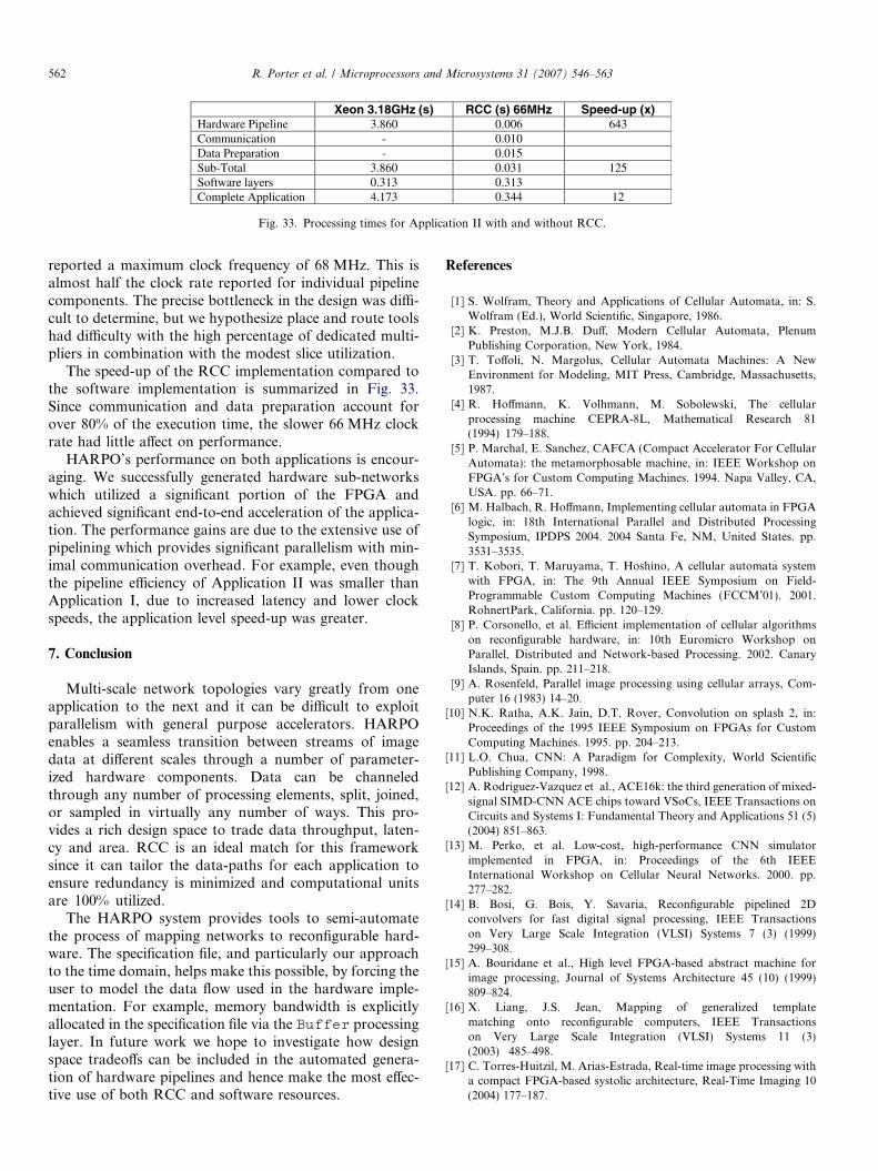
Xeon 3.18GHz (s) RCC (s) 66MHz Speed-up (x) Hardware Pipeline 3.860 0.006 643 Communication 0.010 Data Preparation -

- 0.015

Sub-Total 3.860 0.031 125 Software layers 0.313 0.313 Complete Application 4.173 0.344 12

Fig. 33. Processing times for Application II with and without RCC.


reported a maximum clock frequency of 68 MHz. This isalmost half the clock rate reported for individual pipelinecomponents. The precise bottleneck in the design was diffi-cult to determine, but we hypothesize place and route toolshad difficulty with the high percentage of dedicated multi-pliers in combination with the modest slice utilization.

The speed-up of the RCC implementation compared tothe software implementation is summarized in Fig. 33.Since communication and data preparation account forover 80% of the execution time, the slower 66 MHz clockrate had little affect on performance.

HARPO’s performance on both applications is encour-aging. We successfully generated hardware sub-networkswhich utilized a significant portion of the FPGA andachieved significant end-to-end acceleration of the applica-tion. The performance gains are due to the extensive use ofpipelining which provides significant parallelism with min-imal communication overhead. For example, even thoughthe pipeline efficiency of Application II was smaller thanApplication I, due to increased latency and lower clockspeeds, the application level speed-up was greater.

7. Conclusion

Multi-scale network topologies vary greatly from oneapplication to the next and it can be difficult to exploitparallelism with general purpose accelerators. HARPOenables a seamless transition between streams of imagedata at different scales through a number of parameter-ized hardware components. Data can be channeledthrough any number of processing elements, split, joined,or sampled in virtually any number of ways. This pro-vides a rich design space to trade data throughput, laten-cy and area. RCC is an ideal match for this frameworksince it can tailor the data-paths for each application toensure redundancy is minimized and computational unitsare 100% utilized.

The HARPO system provides tools to semi-automatethe process of mapping networks to reconfigurable hard-ware. The specification file, and particularly our approachto the time domain, helps make this possible, by forcing theuser to model the data flow used in the hardware imple-mentation. For example, memory bandwidth is explicitlyallocated in the specification file via the Buffer processinglayer. In future work we hope to investigate how designspace tradeoffs can be included in the automated genera-tion of hardware pipelines and hence make the most effec-tive use of both RCC and software resources.

References

[1] S. Wolfram, Theory and Applications of Cellular Automata, in: S.Wolfram (Ed.), World Scientific, Singapore, 1986.

[2] K. Preston, M.J.B. Duff, Modern Cellular Automata, PlenumPublishing Corporation, New York, 1984.

[3] T. Toffoli, N. Margolus, Cellular Automata Machines: A NewEnvironment for Modeling, MIT Press, Cambridge, Massachusetts,1987.

[4] R. Hoffmann, K. Volhmann, M. Sobolewski, The cellularprocessing machine CEPRA-8L, Mathematical Research 81(1994) 179–188.

[5] P. Marchal, E. Sanchez, CAFCA (Compact Accelerator For CellularAutomata): the metamorphosable machine, in: IEEE Workshop onFPGA’s for Custom Computing Machines. 1994. Napa Valley, CA,USA. pp. 66–71.

[6] M. Halbach, R. Hoffmann, Implementing cellular automata in FPGAlogic, in: 18th International Parallel and Distributed ProcessingSymposium, IPDPS 2004. 2004 Santa Fe, NM, United States. pp.3531–3535.

[7] T. Kobori, T. Maruyama, T. Hoshino, A cellular automata systemwith FPGA, in: The 9th Annual IEEE Symposium on Field-Programmable Custom Computing Machines (FCCM’01). 2001.RohnertPark, California. pp. 120–129.

[8] P. Corsonello, et al. Efficient implementation of cellular algorithmson reconfigurable hardware, in: 10th Euromicro Workshop onParallel, Distributed and Network-based Processing. 2002. CanaryIslands, Spain. pp. 211–218.

[9] A. Rosenfeld, Parallel image processing using cellular arrays, Com-puter 16 (1983) 14–20.

[10] N.K. Ratha, A.K. Jain, D.T. Rover, Convolution on splash 2, in:Proceedings of the 1995 IEEE Symposium on FPGAs for CustomComputing Machines. 1995. pp. 204–213.

[11] L.O. Chua, CNN: A Paradigm for Complexity, World ScientificPublishing Company, 1998.

[12] A. Rodriguez-Vazquez et al., ACE16k: the third generation of mixed-signal SIMD-CNN ACE chips toward VSoCs, IEEE Transactions onCircuits and Systems I: Fundamental Theory and Applications 51 (5)(2004) 851–863.

[13] M. Perko, et al. Low-cost, high-performance CNN simulatorimplemented in FPGA, in: Proceedings of the 6th IEEEInternational Workshop on Cellular Neural Networks. 2000. pp.277–282.

[14] B. Bosi, G. Bois, Y. Savaria, Reconfigurable pipelined 2Dconvolvers for fast digital signal processing, IEEE Transactionson Very Large Scale Integration (VLSI) Systems 7 (3) (1999)299–308.

[15] A. Bouridane et al., High level FPGA-based abstract machine forimage processing, Journal of Systems Architecture 45 (10) (1999)809–824.

[16] X. Liang, J.S. Jean, Mapping of generalized templatematching onto reconfigurable computers, IEEE Transactionson Very Large Scale Integration (VLSI) Systems 11 (3)(2003) 485–498.

[17] C. Torres-Huitzil, M. Arias-Estrada, Real-time image processing witha compact FPGA-based systolic architecture, Real-Time Imaging 10(2004) 177–187.


[18] Z. Nagy, P. Szolgay, Configurable Multilayer CNN-UM emulator onFPGA, IEEE Transactions on Circuits and Systems-I: FundamentalTheory and Applications 40 (6) (2005) 774–778.

[19] R. Porter et al., Optimizing digital hardware perceptrons for multi-spectral image classification, Journal of Mathematical Imaging andVision 19 (2003) 133–150.

[20] K. Fukushima, Neocognitron: a hierarchical neural network capableof visual pattern recognition, Neural Networks 1 (1988) 119–130.

[21] Y. LeCun et al., Gradient-based learning applied to documentrecognition, Intelligent Signal Processing (2001) 306–351.

[22] T. Serre, L. Wolf, T. Poggio, A New Biologically MotivatedFramework for Robust Object Recognition. CBCL Paper #243/AIMemo #2004-026. 2004, Massachusetts Institute of Technology,Cambridge, MA.

[23] G.S. Vanderwal, P.J. Burt, A VLSI pyramid chip for multiresolutionimage analysis, International Journal of Computer Vision 8 (3) (1992)177–189.

[24] M.A. Nuno-Maganda, M.O. Arias-Estrada, C. Feregrino-Uribe,Three video applications using an FPGA based pyramid implemen-tation: Tracking, Mosaics and Stabilization, in: 2003 IEEE Interna-tional Conference on Field-Programmable Technology (FPT). 2003.Tokyo, Japan, pp. 336–339.

[25] S. Behnke, Hierarchical neural networks for image interpreta-tionLNCS, Vol. 2766, Springer, 2002, p. 224.

[26] N. Woolfries, et al. Non linear image processing on field program-mable gate arrays, in: NOBLESSE Workshop on Non-linear ModelBased Image Analysis. 1998. Glasgow. pp. 301–307.

[27] M. Annapolis, <http://www.annapmicro.com/>. 2001.

http://www.annapmicro.com/

a reconfigurable computing framework for multi-scale cellular image processing

Documents