a quantitative model for option sell-side trading with

A Quantitative Model for Option Sell-Side Tradingwith Stop-Loss Mechanism by Using RandomForestChi-Fang Chao

National Taipei University of TechnologyYu-Chen Wang

National Taipei University of TechnologyMu-En Wu ( [email protected] )

National Taipei University of Technology https://orcid.org/0000-0002-4839-3849

Research Article

Keywords: Option, Trading Strategy, Money Management, Kelly Criterion, Machine Learning

Posted Date: August 6th, 2021

DOI: https://doi.org/10.21203/rs.3.rs-769898/v1

License: This work is licensed under a Creative Commons Attribution 4.0 International License. Read Full License

https://doi.org/10.21203/rs.3.rs-769898/v1

mailto:[email protected]

https://orcid.org/0000-0002-4839-3849

https://doi.org/10.21203/rs.3.rs-769898/v1

https://creativecommons.org/licenses/by/4.0/

Noname manuscript No.(will be inserted by the editor)

A Quantitative Model for Option Sell-Side Trading withStop-Loss Mechanism by Using Random Forest

Chi-Fang Chao · Yu-Chen Wang · Mu-En Wu*

Received: date / Accepted: date

Abstract Due to the characteristics of high leverageand low margin, option is very suitable for quantitative

trading by applying portfolio management to controlthe profit and risk. The money management is an im-portant issue to build a portfolio especially for option

sell-side trader, since the profit is only the premium,

while the loss is unlimited. In this research, we propose

a model for option sell-side strategy to estimate the

win-rate of option by the premium, time to maturity,

and volatility based on statistical approach and ran-dom forest algorithm. The prediction of the model isvisualized through heatmap which can reveal the prof-

itable trading range intuitively, we use the precision

score to evaluate the performance in these two models

and proof the effectiveness and robustness of predictive

model proposed by random forest algorithm. In the fu-

ture, we plan to apply other machine learning algorithm

to propose the predictive model for spread trading.

Keywords Option · Trading Strategy · Money

Management · Kelly Criterion · Machine Learning

�Mu-En Wu* (Corresponding Author)E-mail: [email protected]

Chi-Fang ChaoE-mail: [email protected]

Yu-Chen WangE-mail: [email protected]

Department of Information and Finance Management, Na-tional Taipei University of Technology, Taipei City, Taiwan.

1 Introduction

1.1 Background and motivation

With the evolution of the financial market, investment

tools and trading strategies have become increasinglydiversified. Option is a common and popular deriva-tive financial product, and investors often use it for

hedging or speculation (Merton, 1973). However, op-

tion have the characteristics of high leverage which can

earn higher profits with lower costs, and produce larger

losses. Investors often need to bear higher risk (Yang

et al., 2017). Especially when the option sell-side op-

erates Naked Option, the maximum profit is only the

premium, but the maximum loss is unlimited. When the

market fluctuates sharply, it is easy to be called by the

exchange for margin or forced liquidation (Cox et al.,

1979; Liu et al., 2021). Therefore, fund management

and risk control are particularly important for option

sell-side.

In recent years, the financial market has been tur-

bulent, and the importance of fund management has

become a very importance research topic in both the

industry and academia. For investors, proper fund man-

agement can effectively allocate available funds to var-ious markets or financial products, and further adjustthe size of the funds according to the risk and win-

rate of the transaction, in order to pursue long-term

stable profits. The concept of money management origi-

nated from Kelly Criterion (Kelly Jr, 2011) proposed by

John Larry Kelly in 1956. Which initially used to study

the problem of incomplete message transmission due

to communication noise, and then it was derived into

a formula of the optimal betting ratio (Thorp, 2011;

Stutzer, 2011; Wu et al., 2017). Then, in 2008, Edward

O. Thorp applied the Kelly criterion to blackjack poker

2 C.F. Chao et al.

games, sports betting, and securities markets (Thorp,

2011). The Kelly criterion is applicable to traditional

gambling games with an unlimited number of bets and

a fixed win-rate and odds (Wu et al., 2015). In the case

of a fixed profit-to-loss ratio, the expected value and the

optimal betting ratio can be calculated, and repeated

betting under the condition of a fixed ratio can maxi-

mize the asset growth (MacLean et al., 2011, 2010; Wuet al., 2017). However, there are still many differencesbetween financial trading and traditional gambling, and

it is difficult for real trading to achieve the unlimited

betting. Moreover, the market is unpredictable, and the

win-rate and odds of a trading cannot be completely ac-

curately estimated (Wu et al., 2015). Therefore, if the

Kelly criterion is to be applied to the financial market,

it is necessary to formulate a perfect trading strategy.

This strategy requires fixed odds and as accurately as

possible the probability of winning. In a limited number

of transactions, if the estimated win-rate of the strat-

egy is almost equal to the actual profit ratio, the Kelly

criterion can be applied to calculate the expected value

and the optimal betting ratio.

From the above, there is a gap between the actual

trading and the Kelly criterion applicable to traditional

gambling. However, in many financial commodities. Op-

tion can know the maximum profit and maximum loss

of the transaction through a combination strategy or

a stop-loss method. And then control the transaction

risk and profit (Wu and Chung, 2018; Wu and Hung,

2018). The option of fixing the stop-loss is similar tothe way of the Kelly criterion to fix the odds, so if anaccurate trading win-rate can be obtained. Then theKelly criterion can be applied to the option strategy,

and appropriate capital allocation and position control

can be done (Bermin et al., 2019; Bermin and Holm,

2021). In addition to the fixed odds, the estimation of

the win-rate will be an important factor. If there isan error between the predicted win-rate of the strat-egy and the actual profit probability, it will affect the

long-term capital gains and losses. Therefore, the accu-

racy of win-rate estimation will be one of the important

research topics in this study.

The win-rate is the primary consideration in the

process of making a trading strategy. A high win-rate

means more opportunities for profit. For option trad-

ing, the win-rate of option sell-side is much higher thanthat of option buyers (Evans et al., 2009). In view ofthis, this study will develop trading strategies from the

perspective of option sell-side. Although the option sell-

side has a high win-rate, but the risk is relatively high.

Its maximum profit is only the premium, but the max-

imum loss is unlimited. If there is a sharp rise or fall

during the contract period, the option sell-side may suf-

fer a huge loss. Therefore, the establishment of a stop-

loss mechanism is an important key to the developmentstrategy of this study. If the trading strategy fixes thestop loss point that means we have the odds. Just use

statistical methods or machine learning techniques to

estimate an accurate win-rate (Ruf and Wang, 2020).

The Kelly criterion mentioned above can be applied to

make the best allocation of funds to achieve long-term

stable returns.

1.2 Purposes

Since options have a combination strategy operationmethod, investors can fix their profits and losses (Bren-ner and Subrahmanyam, 1994). This study proposes

a trading strategy for option sell-side with stop-loss

mechanism. Apply the concept of fixed odds of the

Kelly criterion to the strategy, and formulate a pre-

mium doubling stop-loss system to control the risks.

Then, statistical methods and machine learning algo-

rithms are used to estimate the win-rate (Nabipour

et al., 2020; Jang et al., 2021). The model training fea-

ture value mainly uses the premium and the time to ma-

turity and adds the volatility as a filter. Finally, based

on the overall experimental results and the predicted

win-rate of the model, a stable and profitable trading

range was screened out, and the actual feasibility of the

strategy was proved.

2 Preliminaries

2.1 Characteristics of Option

Option is a derivative financial product that investors

often use to hedge or speculate. Option trading is Zero-

Sum Game, and buy-side profit (loss) is the sell-side loss

(profit) (Brenner and Subrahmanyam, 1994). When the

contract is established, the option buy-side has the right

to buy or sell a certain amount of the subject matter at

a certain price on a certain date in the future. In order

to enjoy this right, buy-side must first pay premium to

the sell-side, and sell-side is obliged to perform the con-

tent stipulated in the contract on the expiry date afterreceiving the premium. The option sell-side has obliga-tions but no rights, so it is necessary to pay Margin firstto avoid being unable to perform the contract.

The influencing factors of option value include two:

Intrinsic Value and Time Value. Among them, Time

Value is very important to the option sell-side, so we

will further explain these two values. Intrinsic value

used to determine whether the current price of the op-

tion has a fulfillment value (Wiggins, 1987). As shown

A Quantitative Model for Option Sell-Side Trading with Stop-Loss Mechanism by Using Random Forest 3

in Table 1, suppose we buy a call with a strike price of

12,800. During the contract period, when the index hap-

pens to be at the strike price of 12800, the profit from

the current contract performance will be zero, which

is called ”At the Money”. When the index is less than

the strike price of 12800, the current performance will

cause a loss, which is called ”Out of the Money”. When

the index is greater than the strike price of 12,800, thespread and profit can be made when the contract is ful-filled, which is called ”In the Money”. Therefore, only

the “In the Money” option have the intrinsic value.

Table 1 Comparison table of market index market

and option sell-side profit and loss

Call Strike Price Put

Out of the Money12700

In the Money12750

At the Money 12800 At of the Money

In of the Money12850

Out the Money12900

Time value is like the expectation that the option

buy-side waits for the option to move from “Out of

the Money” to “In the Money”. The in-the-money op-

tion has intrinsic value that can make the buy-side

profitable, while the out-of-the-money option has time

value. When the value of time gradually declines, it

is a moment in favor of the sell-side. It is worth not-ing that as the settlement date approaches, the timevalue of the out-of-the-money option will gradually fade

and approach zero. Option sell-side can earn time value

through the passage of time. When the option premium

returns to zero during settlement, the sell-side makes a

profit, as shown in Figure 1.

Fig. 1 Time value gradually decrease as thesettlement approaches

2.2 Random Forest Algorithm

Random forest is a model training method of ensemblelearning proposed by Leo Breiman, which can be re-

garded as an extension of decision tree (Breiman, 2001).As shown in Figure 2, the method is to randomly takesamples from the data set using Bagging and form mul-tiple decision trees (CART), and the result of each de-

cision tree will form a class (Belgiu and Dragut, 2016;Pal, 2005). The principle of random forest is based on adecision tree as a basic classifier, combining the results

of multiple decision trees, and using voting to select

the category with the most votes among many decision

trees(Pal, 2005). Random forest first uses Bagging to

take samples from the data set and form several de-

cision trees, and then combine many different decisiontrees to form a new learner. Compared with a simpledecision tree, random forest has stronger generalization

ability, can handle more input variables, and can evalu-

ate the importance of each variable. For data sets with

uneven classification, random forest can reduce the er-

ror and less likely to cause overfitting problems. In ad-dition, random forest can also effectively deal with theproblem of missing values. When there are many miss-ing values in the data set, the classification accuracy

can still be maintained through the evaluation method.

Due to the outstanding performance of this algorithm,

its application fields have spread to business analysis, fi-

nancial data, and medical research, etc., and have mademany contributions.

Fig. 2 Schematic for Random Forest Algorithm

3 Methods

In this section, we first introduce the concept of optionsell-side strategy proposed in this paper. Then we esti-

4 C.F. Chao et al.

mate the win-rate with quantitative features by statis-

tical approach and apply heatmap to visualize the win-

rate under with different features. We also propose the

advanced win-rate predictive model based on random

forest algorithm which is one of the popular machine

learning algorithms and the additional quantitative fea-

ture, volatility has been considered in the model.

3.1 Structure for sell-side trading strategy

Due to the naked selling option has the characteristics

of limited profit and unlimited loss, we propose a sell-

side strategy with stop-loss mechanism to constrain the

maximum loss of sell-side option. In this strategy, we

set up the SLR and short the option, the position will

be closed instantly to stop the loss if the premium ofoption rises to (1 + B) times after the trader sold the

option, otherwise the position will be hold to expirationtime, the flowchart of the strategy is shown in Figure3.

Fig. 3 The structure of option sell-side strategy with

stop-loss mechanism

This strategy is composed of short call option and

short put option and only focus on the contract which

time to maturity is less than one week to ensure the

efficiency of fund utilization. T ime to maturity of op-

tion can be represented as {t1, t2, ..., ti, ..., ts}, which tiis the trade time, tj is the stop loss time and ts is theexpiration time, as shown in Fig. 4. If the premium

of option rises to (1 + B) times before ts that is ifCallk,tj ≥ Callk,ti × (1+B) where ti < tj ≤ ts, the po-

sition should be closed to stop the loss or the position

will be hold to ts.

Fig. 4 Schematic for Random Forest Algorithm

Take an example, a sell-side trader shorts a Call

option with strike price of K for 20 at ti and SLR of 1(Callk,ti = 20, SLR = 1), if the premium rises to stop-

loss point 40 (Callk,ti × (1 + B)) on tj , the position

should be closed, or the position will hold to expiration

time ts.

There are three possible outcomes in our sell-side

strategy, supposes a sell-side trader shorts a Call option

with strike price of 10250 for 20 on Monday 10:00 A.M.

and SLR of 1, it can be represented as Short Call10250,Monday10:00A.M.

1, first outcome is if the premium has risen to 40 ontj , the position should be closed, even if the option is

out-of-money at ts, the trader still loss 1,000 dollars(50× 1× 20), as shown in Figure 5(a); second outcome

is the premium of option has not risen to 40 on tj , the

position be hold to expiration and the trader can get1,000 dollars since the out-of-money option does nothave any exercise value, as shown in Figure 5(b); thelast outcome is the premium has rise more than one

times of premium on tj and keep rise until ts, but the

trader has closed the position at stop-loss point, which

could control the maximum loss in 1 times of premium

without the over loss, as shown in Figure 5(c). The de-

scription of the features are shown in Table 2.

Since the maximum loss is controlled by SLR times

of premium and the maximum profit is the premium

only, the odds of the trade have been fixed, we could

estimate the win-lose ratio and measure whether thestrategy with specific features is profitable by expectedvalue calculated by odds and win-lose ratio.

3.2 Win-loss ratio evaluation and visualization

In this section, we use statistical approach to estimate

the win-lose ratio in certain periods based on ODDS

and quantitative features, including TTM and PI. Pre-

mium usually be closed to zero at expiration time, since

the time value decayed accelerates as ts draw closer. Un-less the Premium has risen to (1+B) times, option sell-

side trader can get the full premium paid by buy-side

trader when the Premium is zero, therefore, the mea-

surement of win and lose of the trade is whether the

premium of the option has risen to stop-loss point be-

fore expiration, the win-lose ratio in this section refers

to the ratio of winning times to total times with specific

TTM and PI, which could be defined by Equation 3.1.

win-lose ratioTTM=t,PI=p

=|{∀xin dataset : x > 0}|

|{∀xin dataset}|(1)

In order to verify the feasibility and effectiveness of

our strategy, the data has been separated into training

set and testing set as the comparison and evaluate the


Table 2 Description of the feature

Feature Abbreviation Description

Time to maturity TTM The remaining time of the optionTrade time ti The time that the trader shorts the optionStop-loss time tj The time that the trader closes the option to stop the lossExpiration time ts The time for option settlement to measure whether it has exercise valuePremium Premium The premium of the optionPremium Interval PI The premium interval of the option, each five points is a unitStop-loss ratio SLR The ratio is used to calculate the stop-loss point of premium

(a) The premium has risen to stop-loss point and closes tozero at expiration

(b) The premium has not risen to stop-loss point and closesto zero at expiration

(c) The premium has risen to stop-loss point and above tostop-loss point at expiration

Fig. 5 Possible outcome of the sell-side strategy

win-lose ratio with specific stop-loss ratio by statisti-

cal approach respectively, as shown in Figure 6. Take

short call option for instance, the win-lose ratio can be

expressed by Equation 2.

Prob.{Callk,tj < (1+B)×Callk,ti for all ti < tj ≤ ts}(2)

However, even if Equation 2 is satisfied, the sell-

side trader may still incur losses since Callk,ts might

between 1 and (+B) times of premium, but generally

speaking, Callk,ts less then 5 in most of the time since

the premium usually close to 0 while the option is out-of-money at ts.

Fig. 6 Win-loss ratio estimation based on Premiumand Time to Maturity

With the estimation of win-lose ratio, we utilize the

heatmap to visualize the distribution of win-lose ratio.The vertical axis is PI and the horizontal axis is TTM ,

which is shown in Figure 7. Each block in heatmap

represents the win-lose ratio for strategy with specific

features. Since the benchmark of the color is even win-

lose ratio inferred by fixed odds, the heatmap could

reveal the profitable strategy through the intensity ofthe color.

3.3 Using Random Forest to predict win-rate for our

strategy

Besides to TTM and PI, there still many quantitative

features can be used to estimate the win-lose ratio of

our strategy that whether the premium doubled before

expiration time. However, the computation complexity

will increase dramatically with the number of features

while we use statistical approach, therefore, in order

6 C.F. Chao et al.

Fig. 7 Visualization of win-loss ratio with heatmap

to solve this issue, other estimating approach should

be considered, such as machine learning, neural net-

work and financial engineering etc., these approaches

can take more features into consideration to estimate

the win-rate without worrying about the penalty caused

by computational complexity, the process shown in Fig-ure 8.

Fig. 8 Possible approaches to predict the win-rate

with multiple features

Since we only focus on the option which TTM is

less than one week, the volatility of underlying assethas a significant impact on the premium of the option,therefore, we take volatility as the additional feature to

analyze the influence of volatility on win-rate for the

strategy. Furthermore, since the outcome of whether

premium is doubled before expiration time only can

be classified into two classes, such as doubled and non-

doubled, which is the binary classification problem, there-fore, we select random forest algorithm to propose thepredictive model, which utilizes PI, TTM and volatility

in different frequencies as features to predict whetherthe premium is doubled before expiration time, abbre-viated as is double.

To evaluate the performance of win-rate predictive

model, the data has been divided into training set andtesting set according to the time series. Random forestalgorithm utilizes bootstrap aggregating techniques to

randomly sample the data and features from set with

replacement to generate numbers of decision tree to en-

semble a strong classifier, the principle is shown in Fig-

ure 9. Since each data is classified in one class, we couldpredict the win-rate with specific features in training set

and testing set respectively and make comparison to en-sure the robustness of the predictive model. We also ap-ply confusion matrix which is a commonly used index inmachine learning algorithm to measure the consistency

of predicted outcome and realized outcome.

Fig. 9 Principles of Random Forest Algorithm

4 Experiments

This study used the historical data of Taiwan Stock

Price Index Option (TXO) from June 2017 (after the

implementation of after-hours trading started) to De-

cember 2020 for research. The trading frequency was inminutes, and the close price of per minute was set as thepremium for the option. The call and put option were

be analyzed separately, and the contract period is the

weekly option (settle on every Wednesday). This chap-

ter first used statistical methods to present the distri-

bution of win-rate under fixed odds, and selected prof-

itable trading ranges. Then, apply the random forestalgorithm to focus on the profitable trading range formore in-depth win-rate estimation.

4.1 Using statistical methods to calculate the win-rate

This section reveals the win-lose ratio of statistical ex-

periments. First, we divided the historical data into

training set (data period from June 2017 to December

2019) and testing set (data period from January 2020 to

December 2020). Then use PI and TTM as two major


features, and calculate the win-lose ratio under these

two major features. The win-lose ratio in this study re-

ferred to the ”probability that the premium has not

doubled before expiry”. Therefore, we first marked the

data of ”premium not doubled” in the data as 1, and

the data of ”premium doubled” as 0. After the win-lose

ratio is calculated, heatmap is used to visualize the dis-

tribution result of the win-lose ratio, as shown in Figure10.

Fig. 10 Win-rate heatmap of statistical method

(SLR=1.0)

The top and bottom half of Figure 10 is the heatmap

of win-lose ratio for short call and short put respec-

tively. The vertical axis of the heatmap is PI , from

bottom to top is from 5 to 50 points; and the horizon-

tal axis is the TTM , and the time is in minutes. The

weekly option opens and closes at 08:45 and 13:30 everyWednesday. The total number of minutes in the tradingperiod will be 10365 minutes. Therefore, the horizontal

axis of the heatmap is 10365 (open) to 0 (close) from

left to right, as shown in Figure 11.

Fig. 11 TTM of the weekly option contract

We can measure whether the strategy is profitablebased on the statistical heatmap of win-lose ratio. Take

Figure 10 as an example, the SLR of this heatmap is

set to 1, which means that the stop-loss will be per-

formed immediately when the premium P doubles. Ap-

ply the expected value formula can calculate that when

the odds is 1, the win-rate must be greater than 50 to be

profitable. Therefore, the heatmap in this experiment

will have a corresponding bottom line of win-lose ratio

according to the SLR. If the SLR is 1, the bottom lineof the win-lose ratio will be set to 0.50. If the win-lose

ratio is lower than 0.50, the color in the heatmap will

appear white (unprofitable); on the contrary, if the win-

lose ratio is higher than 0.50, it will appear gradually

red according to the win-rate. From an overall perspec-

tive in Figure 10, short put has a significantly higherwin-lose ratio than short call.

Since financial transactions have the characteristicsof time series, it represents that transaction data iscontinuous and time-sorted random variables. The fre-

quency in this study is in minutes, but the time interval

of high-frequency futures trading is even in seconds. In

order to maintain the characteristics of time continuity

in data, we further apply the concepts of convolution

and smoothing. Think of the heatmap as a small square,and each small square represents the win-rate under theconditions of a specific PI and TTM . In order to re-

duce the gap between adjacent win-lose ratios, we canimagine the heatmap as a lot of nine square grids, andfocus on the center point. Add all the adjacent gridsand divide by 9 to get the average value which is the

convolution win-lose ratio of the strategy. For example,as shown in the red dashed box in Figure 12, the up-per and lower parts of the figure are the ”win-rate of

statistical methods” and ”the win-rate after convolu-

tion” respectively. Let’s take the red box nine square

grid in the statistical method table as an example. The

original win-lose-ratio at the center point (red circle) is

0.42. By adding up the win-lose ratio in the nine square

grid (red dotted box), dividing by the number and tak-

ing the average which is the win-lose ratio of 0.40 after

convolution. As a result, as shown in Figure 13, the top

half and bottom half of the figure are the heatmap of

win-lose ratio for short call and short put respectively.

The vertical axis and horizontal axis of the graph are

also the PI and TTM . After the win-lose ratio of theheatmap is averaged by convolution, the overall win-

lose ratio will become more concentrated and smoother

which helps to select the trading range with a higher

win-rate and stable.

The convolution method not only makes it easier

for us to select the trading range with high win-lose

ratio, but also avoids the problem of squeezing out the

win-lose ratio by cutting the continuity feature value

into segments. As shown in Figure 12, the upper and

lower parts of the figure are the ”win-rate of statis-

tical methods” and ”the winning rate after convolu-

tion” respectively. From the Statistical Method, we can

see that the win-lose ratio of the block with the TTM

between 1265 and 1261 and the PI between 35 and

40 points (the green border) is about 0.62. The win-

8 C.F. Chao et al.

Fig. 12 Comparison of Win-lose ratio between

Statistical and Convolution

Fig. 13 Heatmap after convolution (SLR=1.0)

lose ratio of this block is greater than the expected

value of 0.5, which means it is profitable. However, the

surrounding win-rate is relatively low. As can be seen

from the ”Win-rate after convolution”, the win-rate af-ter smoothing through convolution is about 0.47 (lessthan the expected value of 0.5). If we don’t apply the

convolution method are likely to mistakenly choose an

unstable interval to trade, if there is a slight change in

market conditions is easy to incur losses. In addition, it

is also likely to miss the relatively stable trading range.

As shown in Figure 12, the TTM from the ”statisticalmethods win-lose ratio” is between 1263 and 1259 and

the PI is between 10 and 15 points (the blue border).

A small part of this block has a win-lose ratio less than

the expected value of 0.5, so it is easy to be eliminated.

However, because the win-rate around is relatively high

which can be seen from the ”win-lose ratio after convo-

lution” that the win-rate obtained through the convo-

lution method is about 0.64 (greater than the expected

value of 0.5), which means that this block is stable andprofitable. Therefore, the convolution method can avoidthe problem of squeezing out the win-lose ratio, and

prevent the wrong selection of a high win-lose ratio but

unstable trading range, and then find a truly profitable

range.

From the above, we have obtained a heatmap witha SLR of 1. We also tried several heatmaps with dif-

ferent SLR, including SLR=0.5,1.0,1.5,2.0. The differ-ent SLR will also be matched with their corresponding

bottom line of win-lose ratio. After calculating the ex-

pected value formula, the bottom line of win-lose ratio

is 0.33, 0.50, 0.60, and 0.66 respectively. As shown in

Figure 14, the higher the SLR setting (SLR=2.0), thefewer red dots will be seen (the lower the win-rate), and

the win-rate distribution of the heatmap with B =0.5

is too even. Therefore, the study will use the SLR as 1

for subsequent experiments.

Fig. 14 Comparison of win-lose ratio with different

SLR

We divided the historical data into training set andtesting set. First, we use the training set (from June

2017 to December 2019) to calculate the win-lose ratio,and then use the testing set (from January 2020 to De-cember 2020) to verify the overall effectiveness of the

statistical model. As shown in Figure 15, the left half

and the right half are the heatmap of the training set

and the testing set respectively, while the upper and

lower half are Short Call and Short Put respectively.

This graph still shows that win-lose ratio of Short Put

is much higher than Short Call. Since the risk manage-

ment is also an important issue to our study, both Short

Put and Short Call must be traded at the same time. It

is not possible to trade Short Put only because of the

high win-lose ratio of Short Put. The two are comple-

mentary to each other, it can reduce the risk of large

losses. In order to be able to trade both call and put op-


tions at the same time, it is necessary to choose a high

and stable time interval. Therefore, we choose Monday,

Tuesday, and settlement Wednesday for follow-up ex-

periment and avoid the problem of uncertainty across

the weekend.


dataset

In order to prove that the strategy performance isapplicable, we compare the win-lose ratio of training set

and testing set and measure whether the strategy meets

expectations. As shown in Figure 16, this figure sum-

marizes the win-lose ratio comparison between training

set and testing set in different PI. The top layer andthe bottom layer of the graph is PI with premium of

45 to 50 points and PI with premium of 5 to 10 points,

and the left and right half of the graph are Short Call

and Short Put respectively. The blue polyline and or-

ange polyline are the win-lose ratio of training set and

testing set. We can see from the figure that most of

the training set and testing set win-lose ratio are quite

close. On Tuesday, the win-lose ratio comparison (red

box) with the PI below 30 points, the win-lose ratio

comparison is very close and higher than other weeks.

The result of the comparison of the win-lose ratio in

this figure can show that the trading strategy proposed

by this research is stable and feasible.

4.2 Using random forest algorithm to predict thewin-rate

This section will present the win-rate prediction of the

random forest algorithm. First, due to the win-rateWR

of the trading strategy proposed in this study is defined

as the number of times the premium is ”not doubled”

among all the number of transactions. Therefore, we set

the ”Whether to double” column in the data set as the

classification target of the model. And use PI, TTM

and V olatility as the input features of the model. In

order to experiment with the impact of different fluctu-

ation, we can subdivide the V olatility into the first 1


dataset

minute, 3 minutes, 5 minutes, 15 minutes, 30 minutes,and the first 60 minutes.

Next, in order to evaluate the effectiveness of themodel training, we divided the overall data set (dataperiod from June 2017 to December 2020) in a time se-

ries into 70% for training set and 30% for testing set.

This section will mainly focus on ”Monday, Tuesday,

Settlement Wednesday” to predict the WR with the

random forest model. Before putting the data into the

model, we will first cut every 60 minutes into a segment

based on the TTM . As shown in Figure 17, take Tues-

day as an example. From the opening of the futures

day trading at 08:45 in the morning until the closing of

the night futures trading at 05:00 in the morning of the

next day, the Time to Maturity can be divided into 21

parts for the trading period of Tuesday every 60 min-

utes as a segment. And then put each part of data into

10 C.F. Chao et al.

the model for training, and finally a total of 21 random

forests can be produced based on the data of each time

period. The reason for this approach is that TTM is a

key impact feature of this study. If all the TTM is put

into the model for training at one time, the output of

the experimental results may be too scattered and the

influence of the TTM may decrease. Therefore, dividing

the TTM into small segments according to the numberof minutes can make the reference points of each ran-

dom forest the same and independent and retain the

value of the Time to Maturity.

Fig. 17 Time to Maturity is divided into a random

forest every 60 minutes

When the model training is completed, the test data

will be used for verification. The win-rate represents

the total number of times that each transaction data

is extracted, how many times are estimated to be ”un-

doubled” times. Then, we will merge each of its own

random forests and use the heatmap to present the ex-

perimental results to see the overall win-rate of each

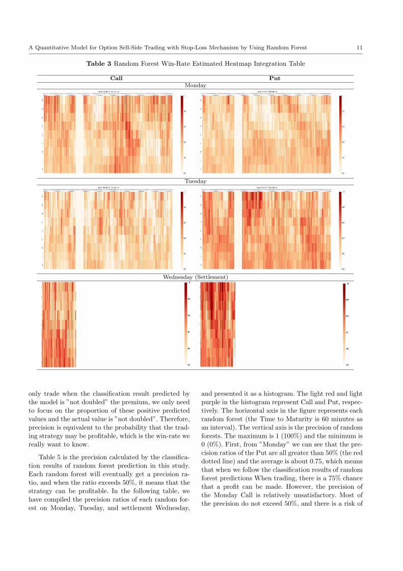
week. As shown in Table 3, the heatmap of the win-

rate predicted by the random forest model on ”Mon-

day, Tuesday and Wednesday (settlement)”. The left

and right sides of the table are the results of Call and

Put respectively, and the vertical axis of each heatmap

in the table is PI, the horizontal axis from left to right

is the TTM from the opening time of the futures daytrading at 08:45 am to the closing time of the futures

night trading at 05:00 am. Only the TTM of Wednes-

day (settlement) only includes the day trading and only

counts until 13:30 at the settlement time. The win-rate

presented from the heatmap represents the result of the

multi-layer judgment made by the algorithm using vari-

ous eigenvalues and the sum of the results. These resultsindicate the number of times that each transaction datahas been classified as ”undoubled” in all forecast cat-egories (including the forecasts as ”not doubled” and

”doubled”). But in fact, we will only conduct trans-

actions on the parts that are ”not doubled”, and ex-

plore the proportion of ”actually not doubled” in these

transactions. This ratio can represent the probability

of a real profit. Therefore, the heatmap in Table 3 can

only show the prediction results of the random forest

model, but this result does not fully represent the win-

rate (profitable probability) we really require.

Using Confusion Matrix allows us to further clar-

ify whether the results predicted by the random forest

model are consistent with actual data, and matrix data

can help us calculate the probability of real profitabil-

ity. Table 4 summarizes the confusion matrix predicted

by the random forest algorithm in this study. The rows

and columns of the confusion matrix represent the pre-

dicted value and the actual value, respectively. Taking

this research as an example, we will observe whetherthe option premium will double before the contract issettled. From the standpoint of the option seller, it is

beneficial to the seller that the premium has not dou-

bled. Therefore, if the actual value of the premium is

”not doubled”, it will be marked as 1, and if the pre-

mium is ”doubled”, it will be marked as 0. The result ofrandom forest prediction is the predicted value. If thepredicted result is that the premium is ”not doubled”,it is classified as 1, and we should enter the market; on

the contrary, if the predicted result is that the premium

is ”doubled”, it is classified Is 0, and we should not take

trading actions.

As shown in Table 4, we have consolidated the con-fusion matrix for Monday, Tuesday, and settlementWednes-

day. The percentages of correct predictions for Call andPut on ”Monday” are 54% and 62%, respectively, indi-cating that 50 to 60% of the predictions are accurate.On the other hand, ”Tuesday” Call and Put accounted

for 59% and 68% of the correctness predictions respec-

tively, indicating that about 60% and 70% of the predic-

tions were accurate. Finally, the correctness forecasts of

”Wednesday (Settlement)” Call and Put accounted for71% and 70% respectively, indicating that 70% of theforecasts were accurate.

But compared to the accuracy of model prediction,

what makes us want to know is the precision of model

prediction. Precision refers to the ratio of correct pre-

dictions among all the results predicted by the model,

that is, the degree of similarity between the predicted

value of the model and the actual reference value. And

”precision” refers to the proportion of the model pre-dicted to be positive and the actual value is also pos-itive, which is equivalent to the degree to which the

predicted value matches the actual value within the

specified range of conditions. Taking this study as an

example, when the random forest model predicts that

the premium classified as positive is ”not doubled”, we

should make a transaction. When the model predicts

that the premium classified as negative is ”doubled”,

we will not take any action. It means that when the

classification result is negative, there will be neither

loss nor profit for the trading strategy. Therefore, we

only need to focus on the classification results predicted

by the model to be positive. In other words, since we


Table 3 Random Forest Win-Rate Estimated Heatmap Integration Table

Call Put

Monday

Tuesday

Wednesday (Settlement)

only trade when the classification result predicted by

the model is ”not doubled” the premium, we only need

to focus on the proportion of these positive predicted

values and the actual value is ”not doubled”. Therefore,

precision is equivalent to the probability that the trad-

ing strategy may be profitable, which is the win-rate we

really want to know.

Table 5 is the precision calculated by the classifica-

tion results of random forest prediction in this study.

Each random forest will eventually get a precision ra-

tio, and when the ratio exceeds 50%, it means that the

strategy can be profitable. In the following table, we

have compiled the precision ratios of each random for-

est on Monday, Tuesday, and settlement Wednesday,

and presented it as a histogram. The light red and light

purple in the histogram represent Call and Put, respec-

tively. The horizontal axis in the figure represents each

random forest (the Time to Maturity is 60 minutes as

an interval). The vertical axis is the precision of random

forests. The maximum is 1 (100%) and the minimum is

0 (0%). First, from ”Monday” we can see that the pre-

cision ratios of the Put are all greater than 50% (the red

dotted line) and the average is about 0.75, which means

that when we follow the classification results of random

forest predictions When trading, there is a 75% chance

that a profit can be made. However, the precision of

the Monday Call is relatively unsatisfactory. Most of

the precision do not exceed 50%, and there is a risk of

12 C.F. Chao et al.

Table 4 Confusion matrix unified table predicted by random forest algorithm

Weekday

CallPut

Confusion MatrixActual Value

Not Doubled Doubled

Mon. Predicted ValueNot Doubled 235943 (48 %)

394317 (59 %)184366 (37 %)

201215 (30 %)

Doubled 42777 (9 %)52467 (8 %)

31132 (6 %)23210 (3 %)

Tues. Predicted ValueNot Doubled 239682 (54 %)

394055 (67 %)146777 (33 %)

159995 (27 %)

Doubled 36842 (8 %)24472 (4 %)

22921 (5 %)7745 (1 %)

Wed. (Settlement) Predicted ValueNot Doubled 49730 (70 %)

53012 (68 %)17505 (25 %)

18758 (24 %)

Doubled 3272 (5 %)4303 (6 %)

877 (1 %)1428 (2 %)

loss. From the data of ”Tuesday”, it can be found that

most of the precision ratios of call rights and put rights

are more than 50%, and the average values are 0.59

and 0.77. Finally, from the histogram of ”Settlement

Wednesday”, we can see that the precision of Call and

Put are both more than 50% and the average values

are 0.70 and 0.74, respectively, indicating that there isa high probability of about 70% of profit. In summary,the prediction precision ratio of most random forest al-gorithms is greater than 50%, and the precision of put

options can be as high as 75% on average. Among them,

the precision data of ”Settlement Wednesday” is the

most ideal.

From precision data, we can know the probability

of a profitable trading strategy. In the process of con-

structing the random forest model, the feature selection

and classification basis of each decision tree in it are

also important influencing factors of the algorithm. The

characteristic values used in the random forest model of

this study include: Premium, TTM and V olatility in

different frequency, including one minutes, three min-

utes, five minutes, fifteen minutes, thirty minutes and

sixty minutes.

Table 6 unifies Monday, Tuesday, and settlementWednesday, and the importance of each feature value

changes with TTM . Each table contains a total of 3graphs, the first and second are the feature importance

line graphs of Call and Put respectively. The vertical

axis of the line graph represents the importance of fea-

tures, the higher the value, the higher the importance;

the horizontal axis represents each random forest. In

the line chart, different line colors respectively repre-

sent a characteristic value, and there are a total of 8different characteristic values. The third graph in eachtable is a bar graph of the feature importance of Call

and Put. The vertical axis represents the value of each

feature, the horizontal axis represents the importance

of the feature. The light red and the light purple in the

horizontal bar graph represents Call and Put respec-

tively. First, from the line and bar charts of ”Monday”

and ”Tuesday”, whether it is a call or a put, the in-

fluence of ”60-minute volatility” ranks first, followed

by ”30-Minute volatility” and ”15-minute volatility”,

volatility is a very important feature. The longer the

volatility time period, the deeper the impact on modelclassification. In addition, from the line chart and barchart of ”Settlement Wednesday”, it can be found that

the importance of the feature of ” Premium” greatly

exceeds other feature values. Time value has a huge

impact on option sell-side. Option sell-side can earn

time value through the passage of time. The time value

of ”Settlement Wednesday” for the option buyer hasdropped rapidly. When the option premium approacheszero at the time of settlement, the seller gains. There-

fore, as the experimental results show, it is reasonable

to interpret that the importance of the feature of ”Pre-

mium” in the random forest model can greatly surpass

other feature values on ”Settlement Wednesday”.

4.3 Comparison of precision between statistical

methods and random forest algorithm

Table 7 is a table of the precision comparison between

statistical methods and random forest prediction. Theleft half and right half of the table are respectively thestatistical model probability to bring 50% and 60% pre-

cision line charts. The vertical axis of the line graph is

the precision, the maximum value is 1 (100%), and the

minimum value is 0 (0%); the horizontal axis is each

random forest. The color of dark red and dark purple

represents the Call and Put of the ”statistical method”

respectively, while the light red and light purple repre-

sent the Call and Put of the ”random forest algorithm”.

First, from the line chart of ”Monday” and ”Tuesday”,


Table 5 Random Forest prediction precision table

Call Put

Mon.

Tues.

Wed. (Settlement)

the precision of the statistical method and the random

forest algorithm are roughly the same, and it can be

found that the precision of Put is significantly higher

than that of Call. In addition, Call and Put are comple-

mentary, whenever one of them has an increased pre-

cision, the other side will decrease which can reduce

the risk of loss. Then, from the line chart of ”Settle-ment Wednesday” at the beginning, the precision ofthe statistical method and the random forest algorithm

is almost the same, but when it is close to the settle-

ment, the precision of the random forest greatly sur-

passes the statistical method. It means that when we

do transactions according to the classification predic-

tion of the random forest, the profit opportunity on

settlement Wednesday is greatly exceeded by the sta-

tistical method, and the precision of the random forest

algorithm can be as high as about 90% when it is close

to the settlement.

5 Conclusions

This paper is devoted to the research and development

of profitable option sell-side trading strategies, and pro-

poses an operating mechanism for stop-loss. In addi-

tion, statistical methods and random forest algorithms

are used to estimate the win-rate of the strategy. The

win-rate represents the proportion of all transactions

that the premium has not doubled before settlement,

and we can also express it with precision. In the experi-

mental results of statistical methods, we found through

the heatmap that the win-rate of Short Put is signifi-

cantly higher than that of Short Call. In order to ex-plore the accuracy of win-rate estimation, we dividedthe data into training set and testing set. The data

results show that the win-rate of the training set and

the testing set are quite close. Among them, the trading

range on Tuesday is the most ideal, and the win-rate can

be as high as about 70%. In addition, in the experimen-

tal results of the random forest algorithm, through the

14 C.F. Chao et al.

Table 6 The importance of features in random forest prediction

Mon.

Tues.

Wed. (Settlement)


Table 7 Comparison of precision between statistical methods and random forest predictions

Weekday Probability Threshold = 50% Probability Threshold = 60%

Mon.

Tues.

Wed. (Settlement)

classification prediction of the model, we found that the

forecast precision of settlement Wednesday is very sat-

isfactory. Both the Call and Put can reach 75%. When

approaching the settlement, the prediction accuracy of

Random Forest can reach nearly 90%, which greatly

surpasses statistical methods. The experimental results

can confirm that the trading strategy proposed by this

paper can effectively achieve risk control through the

development of a stop-loss mechanism with a fixed pre-

mium double multiple. And apply statistical methods

and random forest algorithm to estimate the win-rate

of the strategy, and screen out the trading range with

higher profit and stable. The precision predicted by

the model classification can prove that the strategy is

practical and profitable. In future, we can build mod-

els through more ways, such as neural networks and

financial engineering, and add more different features

for model training. In addition, after we have screenedout profitable trading ranges, we can simulate invest-ment funds and use historical data to do back-testing

and explore the actual profit and loss value. Finally,it is expected that the option sell-side trading strategyproposed in this paper can achieve the desired effect oflong-term stable returns.

Acknowledgements This work was supported in part byMinistry of Science and Technology, R.O.C under grant num-ber MOST 109-2221-E-027 -106 -

Declaration

Conflict of interest

The authors declare that they have no conflict of inter-

est.

Ethical approval

This article doesn’t contain any studies with human

participants or animals performed by any of authors.

16 C.F. Chao et al.

References

Belgiu M, Dragut L (2016) Random forest in remotesensing: A review of applications and future direc-

tions. ISPRS journal of photogrammetry and remote

sensing 114:24–31

Bermin HP, Holm M (2021) Kelly trading and option

pricing. Journal of Futures Markets 41(7):987–1006

Bermin HP, Holm M, et al. (2019) Kelly Trading andMarket Equilibrium. Lund University, School of Eco-

nomics and Management

Breiman L (2001) Random forests. Machine learning

45(1):5–32

Brenner M, Subrahmanyam MG (1994) A simple ap-

proach to option valuation and hedging in the black-

scholes model. Financial Analysts Journal 50(2):25–

28

Cox JC, Ross SA, Rubinstein M (1979) Option pric-

ing: A simplified approach. Journal of financial Eco-

nomics 7(3):229–263Evans RB, Geczy CC, Musto DK, Reed AV (2009)

Failure is an option: Impediments to short selling

and options prices. The Review of Financial Studies

22(5):1955–1980

Jang JH, Yoon J, Kim J, Gu J, Kim HY (2021) Deep-

option: A novel option pricing framework based on

deep learning with fused distilled data from multiple

parametric methods. Information Fusion 70:43–59

Kelly Jr JL (2011) A new interpretation of informationrate. In: The Kelly capital growth investment crite-

rion: theory and practice, World Scientific, pp 25–34

Liu D, Liang Y, Zhang L, Lung P, Ullah R (2021)

Implied volatility forecast and option trading strat-

egy. International Review of Economics & Finance

71:943–954

MacLean LC, Thorp EO, Ziemba WT (2010) Good andbad properties of the kelly criterion. Risk 20(2):1

MacLean LC, Thorp EO, Ziemba WT (2011) The

Kelly capital growth investment criterion: Theory

and practice, vol 3. world scientific

Merton RC (1973) Theory of rational option pricing.The Bell Journal of economics and management sci-

ence pp 141–183Nabipour M, Nayyeri P, Jabani H, Shahab S, Mosavi A

(2020) Predicting stock market trends using machine

learning and deep learning algorithms via continu-

ous and binary data; a comparative analysis. IEEE

Access 8:150199–150212

Pal M (2005) Random forest classifier for remote sens-

ing classification. International journal of remote

sensing 26(1):217–222

Ruf J, Wang W (2020) Neural networks for option pric-

ing and hedging: a literature review. Journal of Com-

putational Finance, Forthcoming

Stutzer M (2011) On growth-optimality vs. securityagainst underperformance. In: The Kelly capital

growth investment criterion: theory and practice,

World Scientific, pp 641–653

Thorp EO (2011) The kelly criterion in blackjack sportsbetting, and the stock market. In: The Kelly capi-

tal growth investment criterion: theory and practice,

World Scientific, pp 789–832

Wiggins JB (1987) Option values under stochastic

volatility: Theory and empirical estimates. Journal

of financial economics 19(2):351–372

Wu ME, Chung WH (2018) A novel approach of optionportfolio construction using the kelly criterion. IEEE

Access 6:53044–53052

Wu ME, Hung PJ (2018) A framework of option buy-

side strategy with simple index futures trading based

on kelly criterion. In: 2018 5th international con-

ference on behavioral, economic, and socio-culturalcomputing (BESC), IEEE, pp 210–212

Wu ME, Tsai HH, Tso R, Weng CY (2015) An adaptive

kelly betting strategy for finite repeated games. In:International conference on genetic and evolutionarycomputing, Springer, pp 39–46

Wu ME, Wang CH, Chung WH (2017) Using trad-

ing mechanisms to investigate large futures data andtheir implications to market trends. Soft Computing21(11):2821–2834

Yang H, Choi HS, Ryu D (2017) Option market char-

acteristics and price monotonicity violations. Journalof Futures Markets 37(5):473–498

a quantitative model for option sell-side trading with

Documents