a $q$-learning approach to derive optimal consumption and investment strategies

1234 IEEE TRANSACTIONS ON NEURAL NETWORKS, VOL. 20, NO. 8, AUGUST 2009

A �-Learning Approach to Derive OptimalConsumption and Investment Strategies

Alex Weissensteiner

Abstract—In this paper, we consider optimal consumption andstrategic asset allocation decisions of an investor with a finite plan-ning horizon. A -learning approach is used to maximize the ex-pected utility of consumption. The first part of the paper presentsconceptually the implementation of -learning in a discrete state-action space and illustrates the relation of the technique to the dy-namic programming method for a simplified setting. In the secondpart of the paper, different generalization methods are exploredand, compared to other implementations using neural networks, acombination with self-organizing maps (SOMs) is proposed. Theresulting policy is compared to alternative strategies.

Index Terms—Asset allocation, dynamic programming, finance,-learning, reinforcement learning, self-organizing maps (SOMs).

I. INTRODUCTION

O NE of the classical problems in finance is to derive op-timal consumption and asset allocation strategies for an

investor with a finite planning horizon. Early work traces backto the pioneering papers of [33], [27], and [28] who focus onanalytical tractability. Since then, a range of different methodshas been proposed in the literature.

Using dynamic programming techniques, one group of pa-pers extends the classical Merton framework along differentlines, e.g., labor income or time-varying investment opportu-nities. Closed-form solutions can be derived only for specialcases (see, e.g., [4], [23], and [40]). Another group proposesapproaches which are not limited in this strict way to analyticaltractability. Their results are exact for a broader set of problemsettings and give approximations in their neighborhood (see,e.g., [8], [9], and [11]). For example, Campbell et al. [8] con-sider Epstein–Zin utility and an infinite planning horizon to-gether with a first-order vector autoregression for the evolutionof asset returns and state variables. Excluding short sale con-straints on the asset allocation, they get an exact solution for thecase of unit elasticity of intertemporal consumption.

To overcome these restrictions of analytical models, variousnumerical methods have been proposed. One approach worksvia a finite-difference approximation on a grid (see, e.g., [1],[7], [13], and [18]) to reduce the state–space dimension andsolve the problem by backward induction. Others, such as De-temple et al. [15] and Brandt et al. [6] use simulation-basedapproaches. While Detemple et al. [15] propose a simulation-

Manuscript received August 04, 2008; revised January 27, 2009; acceptedApril 05, 2009. First published June 02, 2009; current version published Au-gust 05, 2009.This work was supported by the Austrian Nationalbank underJubiläumsfondsprojekt 13054.

The author is with the Department of Banking and Finance, University ofInnsbruck, 6020 Innsbruck, Austria (e-mail: [email protected]).

Digital Object Identifier 10.1109/TNN.2009.2020850

based method to approximate deviations from a closed-form so-lution, Brandt et al. [6] combine Monte Carlo simulation and re-gression techniques, inspired by Longstaff and Schwartz [25].Finally, also stochastic linear programming (SLP), with manysuccessful applications in asset-liability management problems(see, e.g., [14], [17], [19], and [43]), has been proposed to deriveoptimal consumption and investment decisions in the expectedutility framework by [16]. The main advantage of this method isits ability to handle large scale problems with many assets andmany constraints.

However, all these techniques require the specification ofthe dynamics describing the uncertainty of the future, whichdrives asset returns and state variables. For example, in theSLP approach, to maintain computational tractability, themultivariate distribution of the process is approximated with afew mass points (nodes) (see, e.g., [20], [21], and [31]). Giventhis scenario tree optimal decisions are calculated for eachnode. There are at least two conceptual problems when usingthis approach in practical applications (for a discussion, see,e.g., [14]). First, after one period, the realized returns and statevariables are unlikely to coincide exactly with the values in sce-nario tree. Second, the stochastic properties of the process maychange unexpectedly over time. To mitigate these problems,the SLP literature proposes a rolling-forward approach, wherein every stage the new parameters of the stochastic process areestimated and a new scenario tree is generated in order to solvethe optimization task again.1

In this paper, we explore the implementation of -learning[41], [42] to derive optimal consumption and asset allocationdecisions in a finite-horizon model. Compared to the methodsmentioned above, -learning can handle time- and path-depen-dent utility functions and does not require any assumption aboutthe stochastic process. Instead of the rolling-forward approachused, e.g., in the SLP literature, this “online” learning tech-nique allows for continuous adaptation to a changing environ-ment. Like other numerical approaches, -learning also suffersfrom the curse of dimensionality. Therefore, for practical appli-cations, it must be combined with generalization methods. Inthe second part of this paper, we explore function approxima-tion methods (see, e.g., [10], [29], [30], and [39]) and present acombination with self-organizing maps (SOMs) [34], [36]. Thefinite-horizon structure of the problem poses some challenges,as for each decision stage a different map has to be created.

The paper is organized as follows. Section II presents theproblem formulation and relates the optimization task to thewell-known dynamic programming method. Section III studies

1A more comprehensive comparison with other numerical methods is verydemanding and beyond the objective of this paper.

1045-9227/$26.00 © 2009 IEEE

WEISSENSTEINER: A -LEARNING APPROACH TO DERIVE OPTIMAL CONSUMPTION AND INVESTMENT STRATEGIES 1235

conceptually the application of the -learning algorithm forconsumption and asset allocation decisions in a finite-horizoncontext. In Section IV, we give an illustrative example for asimplified task in a discrete state-action space. The general ex-tension to function approximations is explored in Section V,while a combination of -learning with SOMs is proposed inSection VI. In Section VII, results are compared to a case wherea closed-form solution is available. Section VIII concludes.

II. PROBLEM FORMULATION

The objective is to maximize expected utility over a finiteplanning horizon by taking into account optimal consump-tion and investment decisions at discrete points in time (calledstages) from (now) to . In , the last con-sumption and investment decision is made by the individual asat the last stage the individual consumes the remaining wealthcompletely. The optimization task can be formalized in terms ofthe value function

(1)where is a time-additive, strictly concave von Neumann–Mor-genstern utility function, is the time preference rate (for thesake of notation brevity set in the following equal to zero), and

is the total amount of wealth denominated in units of the con-sumption good, which serves as the numeraire. andrefer to the two control variables available at the stages , atwhich the individual has to determine the consumption rateand the asset allocation vector for the remaining financialwealth. The admissible action sets are represented by and

. The uncertainty in the model results from the possi-bility to invest wealth not only in a safe asset, but also in riskyassets. This leads to an -adapted process of wealth . Theexpectation in (1) is with respect to the multivariate distri-bution of the random variables . The corresponding Bellmanequation for this optimization task is given by (see, e.g., [27])

(2)where the migration function describes the transition from thecombination at stage to the wealth at

, i.e., the migration from a given state and given actions toa new state at the following stage when the uncertainty isresolved.

III. -LEARNING

-learning is a reinforcement learning algorithm [41], [42],which calculates the optimal policy in a time-, state-, and action-

discrete environment. Like dynamic programming, -learningis a bootstrapping method, as the update of estimates in isbased on estimates in . As a distinctive feature, however, re-inforcement learning algorithms are simulation based, i.e., theyuse training information to evaluate the actions taken. Neverthe-less, there is a strong interrelation between the -value of theoptimal policy and the value function .

Definition 1: The -value of the optimal policyis defined as the expected utility of

choosing the (not necessary optimal) control variablesand with given wealth at stage and following theoptimal policy afterwards.

In this way, the -function maps state-action combinationsto expected utility

(3)

To see the interrelation between the -function and the valuefunction of the optimal policy, compare (4) and (5)

(4)

(5)

From the above equations, one can verify that the -function ofthe optimal policy corresponds to the value function of theoptimal policy (see, e.g., [35, p. 76])

(6)

and the optimal control variables at stage are given by

(7)

Inserting the corresponding (6) for stage into (4) resultsin (8) shown at the bottom of the page.

-learning, as a simulation-based method, does not requireall possible trajectories and the corresponding probabilities tosolve the control task recursively, but estimates the -values

by an incremental learning approach.This can be done either by simulating single trajectories from

to or by using real market data (see, e.g., [10]). In thesecond case, there is no need to specify a stochastic processor to estimate its parameters (see, e.g., [22]). The estimated

-values for the state-action vectorare maintained in a lookup table and updated

(8)


on occurrence of new experiences , , on this spe-cific combination (see, e.g., [2]) using the incremental updatingformula

(9)

where the vector replaces and indi-cates the learning step size. Convergence of the estimated

-values to the optimal -valuesin (8) would be guaranteed by the law of

large numbers, visiting all state-action pairs infinitely often[42] and by ensuring that satisfies (see [37])

and (10)

In this way, also the actions for the learned policy will convergeto their optimal values; see (7). In Section IV, we set ,satisfying the conditions (10).

Rearranging the ideas and formulas above, we construct the-learning algorithm for a consumption and asset allocation

strategy (Algorithm 1).

Algorithm 1: -learning for a consumption and investmentstrategy

1: Initialize arbitrarily (e.g., with 0)

2: for trajectory to (number of trajectories) do

3: Initialize with the initial wealth

4: for to do

5: Choose a policy to select from(e.g., -greedy policy)

6:

7: if then

8:

9: else

10:

11: end if with for

12: end for

13: end for

Line 8 shows the update of , which is based onthe utility of current consumption and on the esti-mated value of the optimal policy in state by

[see also (6)]. These two determine the new estimation (ortarget) for in (9) and indicate the direction inwhich to move.

IV. RESULTS IN THE DISCRETE STATE-ACTION SPACE

In the following illustrative example, we present a simplifiedtask, where an individual with a time-additive, strictly concavevon Neumann–Morgenstern utility function and initial wealth

wants to take optimal decisions from a set of discrete con-sumption and investment possibilities in order to maximize hisexpected utility over the planning horizon; see (1). We assumethat the market offers two investment opportunities, a risk-freeasset and a risky asset. To model the uncertainty, we further as-sume that at each stage two states of nature canoccur with probabilities , in which the risky assetwill realize the returns or . In this way, the process of therisky asset corresponds to a binomial tree. To avoid dominanceand the ensuing arbitrage opportunities, we set ,where represents the return of the risk free asset. The totalnumber of -values to estimate and updatecan easily be calculated by

(11)

where and are the number of discrete consumption andinvestment possibilities at each stage .

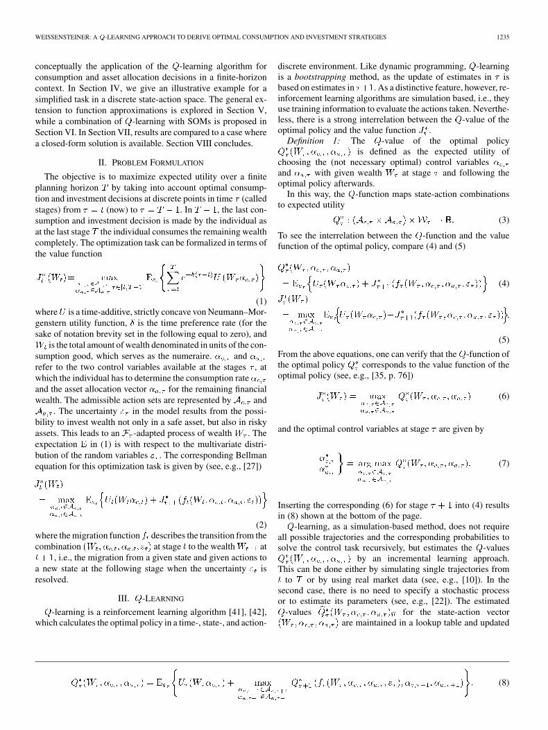
Fig. 1 illustrates the -learning process at a specific stage ,grouping the Cartesian product of consumption and investmentpossibilities, i.e., , on the -axis of the graphs.In the example used here, we allow for three consumption

and three investment possibilities, resultingin a total of nine action combinations for each discrete levelof wealth . On the -axis, we plot the wealth , whilethe -axis shows the corresponding -values. The estimated

-value for the optimal policy is indicatedby a black bullet.

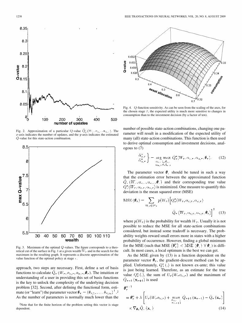
A total of 162 -values are tuned at this specific stage .During the learning process, each of them is updated. For aparticular -combination, these updates areillustrated in Fig. 2. In this way, the rather crumpled -surfacein the top graph of Fig. 1 becomes considerably smoother.Optimal consumption and investment decisions are taken ac-cording to (7). Given wealth , the individual will choose the

-combination with the highest estimated -value, i.e., the combination with the highest

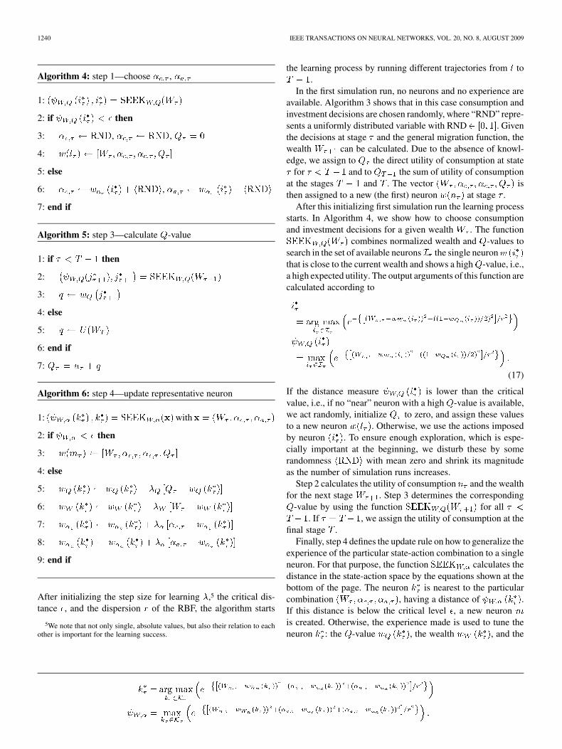
expected utility analogous to the value function of the optimalpolicy; see (6). This corresponds to a theoretical cut of thesurface in Fig. 1 at the given wealth and in the search forthe maximum in the resulting graph. Performing this calcu-lation for all discrete wealth levels and plotting the resulting


Fig. 1. �-learning process at a specific stage � . The graphic illustrates the �-learning process, grouping the Cartesian product of consumption and investmentpossibilities on the �-axis, the wealth on the �-axis, and the �-values on the �-axis. Each estimated �-value for the optimal policy � �� isindicated by a black bullet. During the learning process, they are updated, smoothing the �-surface in the top of the figure.

maximum -values in Fig. 3, we get a (discrete) approximationof the value function of the optimal policy at stage .

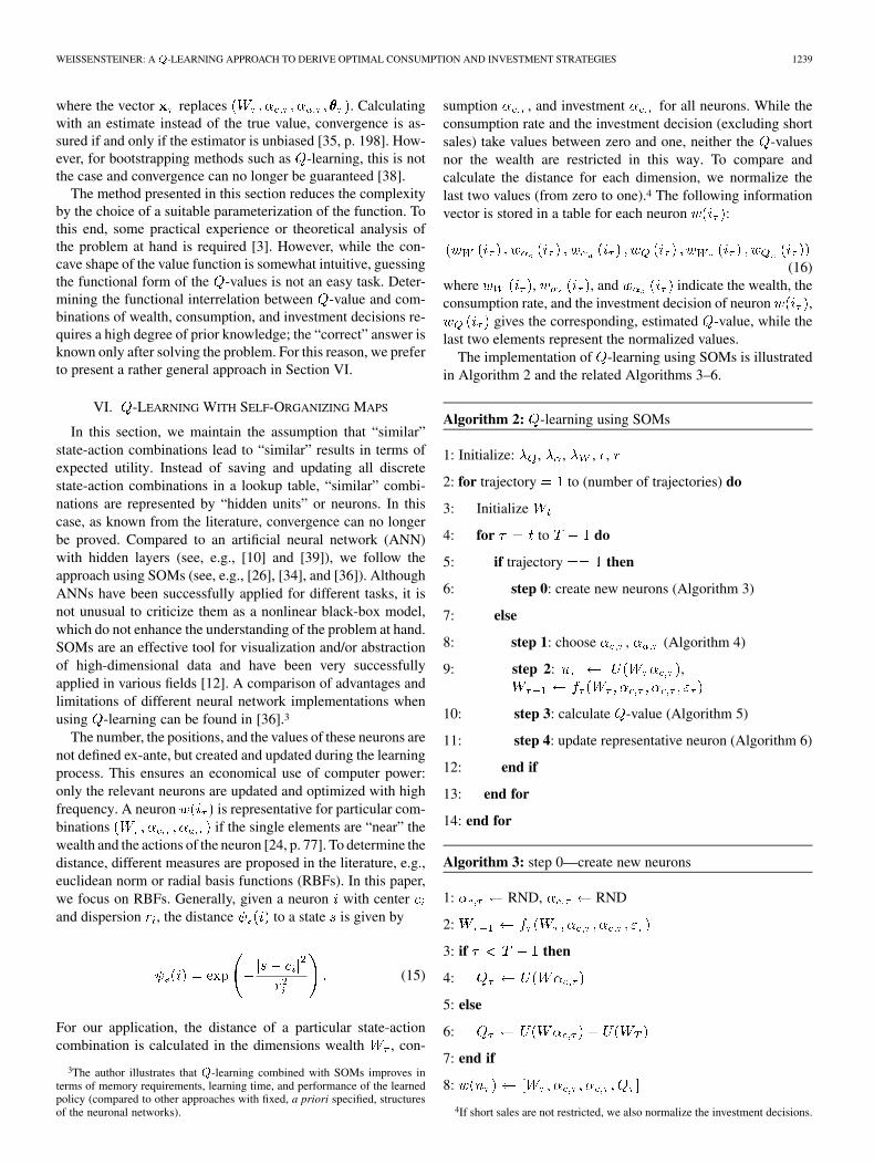
Next, we study the sensitivity of the -valueswith respect to different consumption/in-

vestment combinations at stage . The results are plotted inFig. 4. As can be seen from the scaling of the axes, for thechosen stage , the expected utility is much more sensitive tochanges in consumption than to the investment decision (by afactor of ten).

V. FUNCTION APPROXIMATION

Section IV presented an example for a discrete state-actionspace. For the sake of computational tractability, we restricted

the problem in two ways: the process of the risky asset wasmodeled by a binomial tree and the sets of consumption andinvestment possibilities were each limited to three elements, asthe computational complexity increases exponentially; see (11).For high-dimensional and continuous state-action spaces, someform of generalization is required [5]. Generalization methodsassume that “similar” wealth at a given stage will lead to“similar” expected utility. In this way, a compact storage oflearned information and a transfer of knowledge between “sim-ilar” states and actions can be established [22]. A classical formof generalization is function approximation.

Instead of saving all possible combinations at stage in alookup table, the -values are calculated by a function. For this


Fig. 2. Approximation of a particular �-value � �� . The�-axis indicates the number of updates, and the �-axis indicates the estimated�-value for this state-action combination.

Fig. 3. Maximum of the optimal �-values. The figure corresponds to a theo-retical cut of the surface in Fig. 1 at a given wealth � and in the search for themaximum in the resulting graph. It represents a discrete approximation of thevalue function of the optimal policy at stage � .

approach, two steps are necessary. First, define a set of basisfunctions to calculate . The intuition orunderstanding of a user in providing this set of basis functionsis the key to unlock the complexity of the underlying decisionproblem [32]. Second, after defining the functional form, esti-mate (or “learn”) the parameter vector .2

As the number of parameters is normally much lower than the

2Note that for the finite horizon of the problem setting this vector is stagedependent.

Fig. 4. �-function sensitivity. As can be seen from the scaling of the axes, forthe chosen stage � , the expected utility is much more sensitive to changes inconsumption than to the investment decision (by a factor of ten).

number of possible state-action combinations, changing one pa-rameter will result in a modification of the expected utility ofmany (all) state-action combinations. This function is then usedto derive optimal consumption and investment decisions, anal-ogous to (7)

(12)

The parameter vector should be tuned in such a waythat the estimation error between the approximated function

and their corresponding true valueis minimized. One measure to quantify this

deviation is the mean squared error (MSE)

(13)

where is the probability for wealth . Usually it is notpossible to reduce the MSE for all state-action combinationsconsidered, but instead some tradeoff is necessary. The prob-ability weights reward small errors more in states with a higherprobability of occurrence. However, finding a global minimumfor the MSE (such that MSE ) is diffi-cult. In most cases, a local optimum is the best we can get.

As the MSE given by (13) is a function dependent on theparameter vector , the gradient-descent method can be ap-plied. Unfortunately, is not known ex-ante; this valueis just being learned. Therefore, as an estimate for the truevalue , the sum of and the maximum of

is used

(14)


where the vector replaces . Calculatingwith an estimate instead of the true value, convergence is as-sured if and only if the estimator is unbiased [35, p. 198]. How-ever, for bootstrapping methods such as -learning, this is notthe case and convergence can no longer be guaranteed [38].

The method presented in this section reduces the complexityby the choice of a suitable parameterization of the function. Tothis end, some practical experience or theoretical analysis ofthe problem at hand is required [3]. However, while the con-cave shape of the value function is somewhat intuitive, guessingthe functional form of the -values is not an easy task. Deter-mining the functional interrelation between -value and com-binations of wealth, consumption, and investment decisions re-quires a high degree of prior knowledge; the “correct” answer isknown only after solving the problem. For this reason, we preferto present a rather general approach in Section VI.

VI. -LEARNING WITH SELF-ORGANIZING MAPS

In this section, we maintain the assumption that “similar”state-action combinations lead to “similar” results in terms ofexpected utility. Instead of saving and updating all discretestate-action combinations in a lookup table, “similar” combi-nations are represented by “hidden units” or neurons. In thiscase, as known from the literature, convergence can no longerbe proved. Compared to an artificial neural network (ANN)with hidden layers (see, e.g., [10] and [39]), we follow theapproach using SOMs (see, e.g., [26], [34], and [36]). AlthoughANNs have been successfully applied for different tasks, it isnot unusual to criticize them as a nonlinear black-box model,which do not enhance the understanding of the problem at hand.SOMs are an effective tool for visualization and/or abstractionof high-dimensional data and have been very successfullyapplied in various fields [12]. A comparison of advantages andlimitations of different neural network implementations whenusing -learning can be found in [36].3

The number, the positions, and the values of these neurons arenot defined ex-ante, but created and updated during the learningprocess. This ensures an economical use of computer power:only the relevant neurons are updated and optimized with highfrequency. A neuron is representative for particular com-binations if the single elements are “near” thewealth and the actions of the neuron [24, p. 77]. To determine thedistance, different measures are proposed in the literature, e.g.,euclidean norm or radial basis functions (RBFs). In this paper,we focus on RBFs. Generally, given a neuron with centerand dispersion , the distance to a state is given by

(15)

For our application, the distance of a particular state-actioncombination is calculated in the dimensions wealth , con-

3The author illustrates that �-learning combined with SOMs improves interms of memory requirements, learning time, and performance of the learnedpolicy (compared to other approaches with fixed, a priori specified, structuresof the neuronal networks).

sumption , and investment for all neurons. While theconsumption rate and the investment decision (excluding shortsales) take values between zero and one, neither the -valuesnor the wealth are restricted in this way. To compare andcalculate the distance for each dimension, we normalize thelast two values (from zero to one).4 The following informationvector is stored in a table for each neuron :

(16)where , , and indicate the wealth, theconsumption rate, and the investment decision of neuron ,

gives the corresponding, estimated -value, while thelast two elements represent the normalized values.

The implementation of -learning using SOMs is illustratedin Algorithm 2 and the related Algorithms 3–6.

Algorithm 2: -learning using SOMs

1: Initialize: , , , ,

2: for trajectory to (number of trajectories) do

3: Initialize

4: for to do

5: if trajectory then

6: step 0: create new neurons (Algorithm 3)

7: else

8: step 1: choose , (Algorithm 4)

9: step 2: ,

10: step 3: calculate -value (Algorithm 5)

11: step 4: update representative neuron (Algorithm 6)

12: end if

13: end for

14: end for

Algorithm 3: step 0—create new neurons

1: RND, RND

2:

3: if then

4:

5: else

6:

7: end if

8:

4If short sales are not restricted, we also normalize the investment decisions.


Algorithm 4: step 1—choose ,

1:

2: if then

3: , ,

4:

5: else

6: ,

7: end if

Algorithm 5: step 3—calculate -value

1: if then

2:

3:

4: else

5:

6: end if

7:

Algorithm 6: step 4—update representative neuron

1: with

2: if then

3:

4: else

5:

6:

7:

8:

9: end if

After initializing the step size for learning ,5 the critical dis-tance , and the dispersion of the RBF, the algorithm starts

5We note that not only single, absolute values, but also their relation to eachother is important for the learning success.

the learning process by running different trajectories from to.

In the first simulation run, no neurons and no experience areavailable. Algorithm 3 shows that in this case consumption andinvestment decisions are chosen randomly, where “RND” repre-sents a uniformly distributed variable with RND . Giventhe decisions at stage and the general migration function, thewealth can be calculated. Due to the absence of knowl-edge, we assign to the direct utility of consumption at state

for and to the sum of utility of consumptionat the stages and . The vector isthen assigned to a new (the first) neuron at stage .

After this initializing first simulation run the learning processstarts. In Algorithm 4, we show how to choose consumptionand investment decisions for a given wealth . The function

combines normalized wealth and -values tosearch in the set of available neurons the single neuronthat is close to the current wealth and shows a high -value, i.e.,a high expected utility. The output arguments of this function arecalculated according to

(17)

If the distance measure is lower than the criticalvalue, i.e., if no “near” neuron with a high -value is available,we act randomly, initialize to zero, and assign these valuesto a new neuron . Otherwise, we use the actions imposedby neuron . To ensure enough exploration, which is espe-cially important at the beginning, we disturb these by somerandomness with mean zero and shrink its magnitudeas the number of simulation runs increases.

Step 2 calculates the utility of consumption and the wealthfor the next stage . Step 3 determines the corresponding

-value by using the function for all. If , we assign the utility of consumption at the

final stage .Finally, step 4 defines the update rule on how to generalize the

experience of the particular state-action combination to a singleneuron. For that purpose, the function calculates thedistance in the state-action space by the equations shown at thebottom of the page. The neuron is nearest to the particularcombination , having a distance of .If this distance is below the critical level , a new neuronis created. Otherwise, the experience made is used to tune theneuron : the -value , the wealth , and the


decision variables and are updated toward, , , and . After some tuning period, consumption

and investment decisions can be selected according to neuronin (17).

In order to speed up learning in Algorithm 2, we propose twofurther improvements. First, as the -value measures expectedutility, we simulate more than one successor for the combina-tion and take the arithmetic mean of the re-sulting -values, instead of calculating step 2 and step 3 onlyfor one . This expected value is used in step 4 to updateour knowledge. Second, as the -value and the wealth are in-terrelated (the higher the wealth, the higher the expected utilityexpressed in terms of the -value), we divide the set intwo subsets: whose neurons have a wealth below ,and with a higher wealth. In both sets, we use (17) to find aneuron nearby and interpolate linearly their -values to approx-imate the value of wealth . Without such a correction, wewould have a bias in the estimates: given two neurons equallydistant from and both just tuned to the optimal policy,(17) will always choose the one with the higher wealth and thecorresponding higher -value.

VII. RESULTS USING SELF-ORGANIZING MAPS

In the following, we study the application of the algorithmproposed in Section VI. In order to compare the performance ofthe learned policy with the optimal policy, we choose a simpli-fied setting with four stages where a closed-form solution ex-ists. Hence, we use log utility, a risk-free rate set to 4%, andthe risky asset following a geometric Brownian motion (GBM)with a drift of 8% and volatility of 25%. From the lit-erature, we know that in this case the optimal consumption rateis given by the fraction , i.e., 25% at the first stage,and the optimal asset allocation to the risky asset is myopic with

, i.e., 64%.For the learning period, we use 20 000 simulated trajectories

and set the learning parameters by manual tuning to

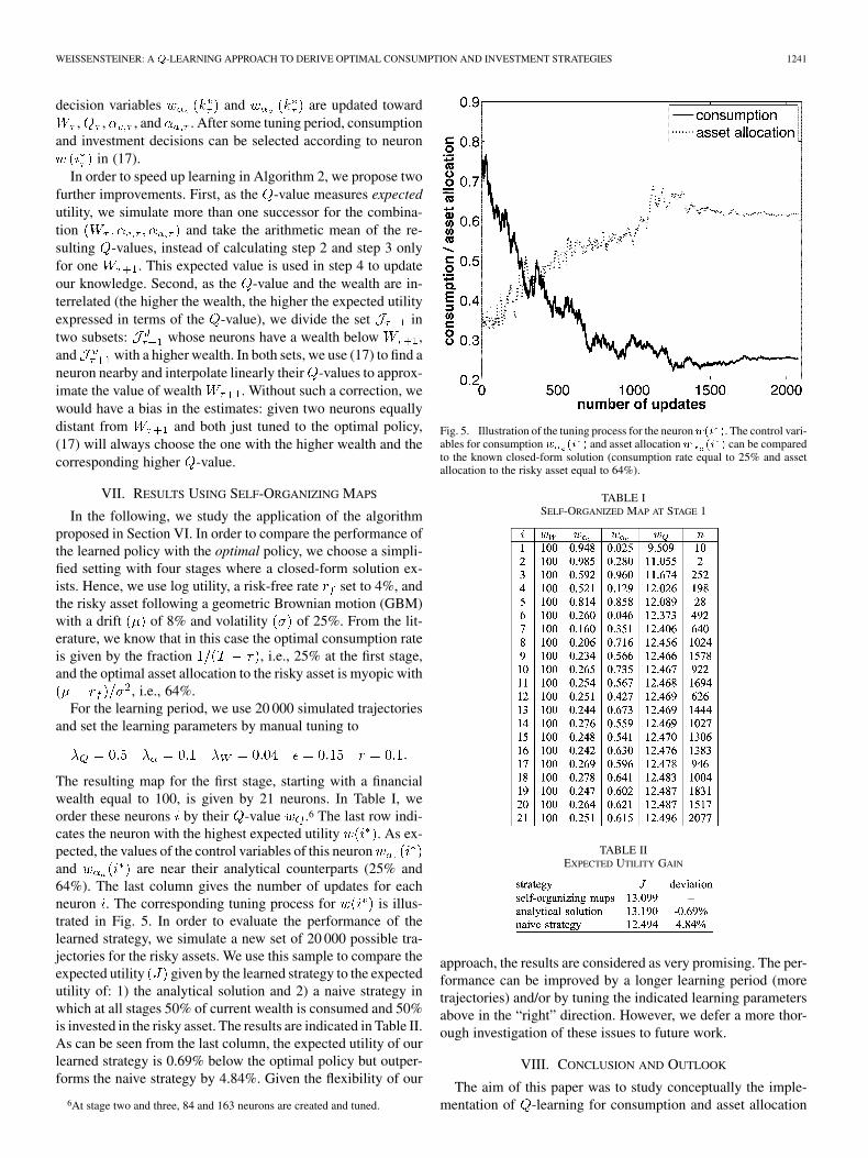
The resulting map for the first stage, starting with a financialwealth equal to 100, is given by 21 neurons. In Table I, weorder these neurons by their -value .6 The last row indi-cates the neuron with the highest expected utility . As ex-pected, the values of the control variables of this neuronand are near their analytical counterparts (25% and64%). The last column gives the number of updates for eachneuron . The corresponding tuning process for is illus-trated in Fig. 5. In order to evaluate the performance of thelearned strategy, we simulate a new set of 20 000 possible tra-jectories for the risky assets. We use this sample to compare theexpected utility given by the learned strategy to the expectedutility of: 1) the analytical solution and 2) a naive strategy inwhich at all stages 50% of current wealth is consumed and 50%is invested in the risky asset. The results are indicated in Table II.As can be seen from the last column, the expected utility of ourlearned strategy is 0.69% below the optimal policy but outper-forms the naive strategy by 4.84%. Given the flexibility of our

6At stage two and three, 84 and 163 neurons are created and tuned.

Fig. 5. Illustration of the tuning process for the neuron�� . The control vari-ables for consumption � �� and asset allocation � �� can be comparedto the known closed-form solution (consumption rate equal to 25% and assetallocation to the risky asset equal to 64%).

TABLE ISELF-ORGANIZED MAP AT STAGE 1

TABLE IIEXPECTED UTILITY GAIN

approach, the results are considered as very promising. The per-formance can be improved by a longer learning period (moretrajectories) and/or by tuning the indicated learning parametersabove in the “right” direction. However, we defer a more thor-ough investigation of these issues to future work.

VIII. CONCLUSION AND OUTLOOK

The aim of this paper was to study conceptually the imple-mentation of -learning for consumption and asset allocation


decisions. Many intuitive results were deduced from the figuresin Section IV. The main advantages of -learning are as fol-lows. First, time- and path-dependent utility functions, whichnormally are problematic for analytical tractability, can easilybe incorporated in the model. Second, the possibility to use thealgorithm without specifying the underlying stochastic processmakes this technique a candidate for online learning with realmarket data, where little is known about the driving parametersand where a changing market environment is the rule rather thanthe exception.

In the illustrative example of Section IV, we have assumedthat the estimates of the -values are represented by a tablewith one entry for each combination. This isa clear and instructive case, but it is limited to a task with asmall number of states and actions. The exponential growthof possible future wealth levels may lead to serious time andmemory problems in the calculation, known as the curse ofdimensionality. In this case, most -values will suffer frompoor updates as they will be reached rarely or never during thelearning process. However, also in this case, another argumentcan be reported in favor of -learning. The forward approachof -learning going from stage to ensures an “efficient use”of computer power: only the practically relevant combinations

, which are encountered often in the state-ac-tion space, are estimated with high accuracy.

Overall, -learning is most attractive when one is faced witha large and complex system which requires approximation: thesimulated trajectories are used to estimate a -function for con-tinuous state-action spaces, rather than to update explicitly everystate-action pair.

In the second part of the paper, we have illustrated the com-bination of -learning with SOMs. Compared to function ap-proximation methods, where after choosing the functional formthe parameter vector is tuned, SOMs try to set and calibrate afinite number of neurons to deduce an optimal strategy. The re-sults seem promising for future work.

ACKNOWLEDGMENT

The author would like to thank A. Geyer, M. Hanke, A. Matt,and G. Regensburger for helpful comments.

REFERENCES

[1] N. C. Barberis, “Investing for the long run when returns are pre-dictable,” J. Finance, vol. 55, pp. 225–264, 2000.

[2] D. P. Bertsekas, Dynamic Programming and Optimal Control. Bel-mont, MA: Athena Scientific, 1995, vol. 2.

[3] D. P. Bertsekas and J. N. Tsitsiklis, Neuro-Dynamic Programming.Belmont, MA: Athena Scientific, 1996.

[4] Z. Bodie, R. C. Merton, and W. F. Samuelson, “Labor supply flexibilityand portfolio choice in a life cycle model,” J. Econom. Dyn. Control,vol. 16, pp. 427–449, 1992.

[5] J. A. Boyan and A. W. Moore, “Generalization in reinforcementlearning: Safely approximating the value function,” in Advances inNeural Information Processing Systems, G. Tesauro, D. S. Touretzky,and T. K. Leen, Eds. Cambridge, MA: MIT Press, 1995.

[6] M. W. Brandt, A. Goyal, P. Santa-Clara, and J. R. Stroud, “A sim-ulation approach to dynamic portfolio choice with an application tolearning about return predictability,” Rev. Financial Studies, vol. 18,no. 3, pp. 831–873, 2005.

[7] M. J. Brennan, E. S. Schwartz, and R. Lagnado, “Strategic asset allo-cation,” J. Econom. Dyn. Control, vol. 21, pp. 1377–1403, 1997.

[8] J. Y. Campbell, Y. L. Chan, and L. M. Viceira, “A multivariate modelof strategic asset allocation,” J. Financial Econom., vol. 67, pp. 41–80,2003.

[9] J. Y. Campbell and L. M. Viceira, “Who should buy long-term bonds?,”Amer. Econom. Rev., vol. 91, no. 1, pp. 99–127, 2001.

[10] P. X. Casqueiro and A. J. Rodrigues, “Neuro-dynamic tradingmethods,” Eur. J. Operat. Res., vol. 175, pp. 1400–1412, 2006.

[11] G. Chacko and L. M. Viceira, “Dynamic consumption and portfoliochoice with stochastic volatility in incomplete markets,” Rev. FinancialStudies, vol. 18, no. 2, pp. 1369–1402, 2005.

[12] F.-J. Chang, L.-C. Chang, and Y.-S. Wang, “Enforced self-organizingmap neural networks for river flood forecasting,” Hydrological Pro-cesses, vol. 21, pp. 741–749, 2007.

[13] J. F. Cocco, F. J. Gomes, and P. J. Maenhout, “Consumption and port-folio choice over the life cycle,” Rev. Financial Studies, vol. 18, no. 2,pp. 491–533, 2005.

[14] M. A. H. Dempster, M. Germano, E. A. Medova, and M. Villaverde,“Global asset liability management,” British Actuarial J., vol. 9, pp.137–216, 2003.

[15] J. B. Detemple, R. Garcia, and M. Rindisbacher, “A Monte Carlomethod for optimal portfolios,” J. Finance, vol. 58, pp. 401–446, 2003.

[16] A. Geyer, M. Hanke, and A. Weissensteiner, “Life-cycle asset alloca-tion and optimal consumption using stochastic linear programming,” J.Comput. Finance, vol. 12, no. 4, pp. 1–22, 2009.

[17] A. Geyer and W. T. Ziemba, “The Innovest Austrian pension fund fi-nancial planning model InnoALM,” Operat. Res., vol. 56, pp. 797–810,2007.

[18] F. Gomes and A. Michaelides, “Optimal life-cycle asset allocation: Un-derstanding the empirical evidence,” J. Finance, vol. 60, pp. 869–904,2005.

[19] J. Gondzio and R. Kouwenberg, “High performance computing forasset-liability management,” Operat. Res., vol. 49, pp. 879–891, 2001.

[20] H. Heitsch and W. Römisch, “Scenario reduction algorithms in sto-chastic programming,” Comput. Optim. Appl., vol. 24, pp. 187–206,2003.

[21] H. K. øyland and S. W. Wallace, “Generating scenario trees for mul-tistage decision problems,” Manage. Sci., vol. 47, no. 2, pp. 295–307,2001.

[22] L. P. Kaelbling, M. L. Littman, and A. W. Moore, “Reinforcementlearning: A survey,” J. Artif. Intell. Res., vol. 4, pp. 237–285, 1996.

[23] T. S. Kim and E. Omberg, “Dynamic nonmyopic portfolio behavior,”Rev. Financial Studies, vol. 9, pp. 141–161, 1996.

[24] T. Kohonen, Self-Organizing Maps. New York: Springer-Verlag,1995.

[25] F. Longstaff and E. Schwartz, “Valuing American options by simula-tion: A simple least-square approach,” Rev. Financial Studies, vol. 14,no. 1, pp. 113–147, 2001.

[26] A. Matt and G. Regensburger, “An adaptive clustering method formodel-free reinforcement learning,” in Proc. IEEE 8th Int. MultitopicConf., 2004, pp. 362–367.

[27] R. C. Merton, “Lifetime portfolio selection under uncertainty: Thecontinuous-time case,” Rev. Economics and Statistics, vol. 51, pp.247–257, 1969.

[28] R. C. Merton, “Optimum consumption and portfolio rules in a contin-uous-time model,” J. Econom. Theory, vol. 3, pp. 373–413, 1971.

[29] J. Moody and M. Saffell, “Learning to trade via direct reinforcement,”IEEE Trans. Neural Netw., vol. 12, no. 4, pp. 875–889, Jul. 2001.

[30] R. Neuneiner, “Optimal asset allocation using adaptive dynamic pro-gramming,” in Advances in Neural Information Processing Systems, D.S. Touretzky, M. C. Mozer, and M. E. Hasselmo, Eds. Cambridge,MA: MIT Press, 1996, pp. 952–958.

[31] G. C. Pflug, “Optimal scenario tree generation for multiperiod financialplanning,” Math. Programm., vol. 89, no. 2, pp. 25–271, 2001.

[32] S. Roy, “Theory of dynamic portfolio choice for survival under uncer-tainty,” Math. Social Sci., vol. 30, pp. 171–194, 1995.

[33] P. A. Samuelson, “Lifetime portfolio selection by dynamic stochasticprogramming,” Rev. Econom. Statist., vol. 51, pp. 239–246, 1969.

[34] J. M. Santos and C. Touzet, “Exploration tuned reinforcement func-tion,” Neurocomputing, vol. 28, pp. 93–105, 1999.

[35] R. S. Sutton and A. G. Barto, Reinforcement Learning: An Introduc-tion. Cambridge, MA: MIT Press, 2000.

[36] C. Touzet, “Neural reinforcement learning for behaviour synthesis,”Robot. Autonom. Syst., vol. 22, Special Issue on Learning Robot: TheNew Wave, no. 3, pp. 251–281, 1997.

[37] J. N. Tsitsiklis, “Asynchronous stochastic approximation and�-learning,” Mach. Learn., vol. 16, pp. 185–202, 1994.


[38] J. N. Tsitsiklis and B. V. Roy, “An analysis of temporal-differencelearning with function approximation,” IEEE Trans. Autom. Control,vol. 42, no. 5, pp. 674–690, May 1997.

[39] N. J. van Eck and M. van Wezel, “Application of reinforcement learningto the game of Othello,” Comput. Operat. Res., vol. 35, pp. 1999–2017,2008.

[40] J. Wachter, “Portfolio and consumption decisions under mean-re-verting returns: An exact solution,” J. Financial Quantitative Anal.,vol. 37, no. 1, pp. 63–91, 2002.

[41] C. J. Watkins, “Learning from delayed rewards,” Ph.D. dissertation,Psychol. Dept., Cambridge Univ., Cambridge, U.K., 1989.

[42] C. J. Watkins and P. Dayan, “�-learning,” Mach. Learn., vol. 8, pp.279–292, 1992.

[43] W. T. Ziemba and J. Mulvey, Worldwide Asset and Liability Mod-eling. Cambridge, U.K.: Cambridge Univ. Press, 1998.

Alex Weissensteiner was born in Bolzano, Italy,on August 20, 1974. He received the M.Sc. andPh.D. degrees in social and economic sciences fromLeopold Franzens University, Innsbruck, Austria, in1998 and 2003, respectively.

Since 2006 he has been a Research Assistant atthe Department of Banking and Finance, LeopoldFranzens University. His research interests includestochastic (linear) programming, control theory,neural networks, and financial risk management.

a $q$-learning approach to derive optimal consumption and investment strategies

Documents