Effects of Hills on the Dynamics of Pyroclastic Density Currents, Mt. St. Helens, Washington

A Project by

Sean B O’Donnell

The University of Texas at Austin

Jackson School of Geosciences

Department of Geological Sciences

GIS and GPS Applications, Fall 2017

Abstract

The lateral blast of the May 1980 eruption of Mt. St. Helens created a large pyroclastic density current that flattened millions of trees north of the volcano. Near the edges of the blast area, it appears that some small hills affected the direction and internal dynamics of the currents as they encountered the hills. Mapping the direction of the trees around these hills shows how the currents reacted and changed direction once they encountered the hills. The direction of the blown-down trees seems to correspond only to the change in current direction and resultant eddy formation, not to any other aspect of the topography.

Problem

The May 18, 1980 eruption of Mt. St. Helens (MSH), Washington was different from many other Plinian eruptions of its kind. Instead of erupting a buoyant, rising column of ash, the north flank of the volcano collapsed at the beginning of the eruption, creating a lateral blast that turned into a (possibly two) really large pyroclastic density current (PDC) that quickly ravaged an area north of the volcano. In the path of the PDC were millions of conifer trees, which sustained different levels of damage depending on location. Closest to the volcano, the trees were buried and destroyed (or ended up floating Spirit Lake following a small tsunami caused by the giant landslide). Across most of the impacted area, the trees were burnt and knocked over (the blow-down zone), and at the edge of the area, where the PDC began to lift-off into a co-ignimbrite cloud, the trees were just burnt but not knocked over (the burnt zone). Within the blow-down zone, there lies some intriguing problems. In some area, out near the edge of the blow-down zone, there are small hills with burnt but still-standing trees on them. This indicates that at this point, the current was hot enough to burn the trees but did not have enough momentum (or something else occurred) to knock them down. Using ArcGIS to examine these areas of the blow-down zone can provide detail about the impact of changes in topography, especially these hills, on the internal dynamics of PDCs.

The trees blow down in the direction the current is moving, so mapping the trees in air photos taken soon after the eruption should tell provide information about the dynamics of the PDC. The hills toward the far end of the blow-down zone should have an impact on the PDC, as the current is losing momentum (compared to closer to the volcano) and is about to become buoyant. Statistics will be used to show how the dynamics of the current were affected by the hills.

Data Collection

In order to map the downed trees, three aerial images taken a few months after the eruption were downloaded from the USGS EarthExplorer database. These images are not orthophotos, nor are they spatially referenced. The process of spatial referencing requires using other data that is spatially referenced to compare the photos to. The state of Washington boundary and county boundary shapefiles were downloaded to create the working space. This followed with the Washington public roads data and the Washington hydrographic data to provide more reference points for the air photos.

Next, 10-meter DEM data for the Mt. St. Helens area was acquired. Multiple DEMs were required, as each DEM only covered the area of 7.5’ quadrangle. 15 DEMs in total were downloaded and used in the project. The other piece of data used for referencing is the USGS map of the eruption deposits made shortly after the eruption. It also had to be spatially referenced. All of the datasets downloaded and used are listed in Table 1.

Data File Type Source Air Photos TIF USGS EarthExplorer

https://earthexplorer.usgs.gov/ Geologic Map

PDF USGS Report 1250 https://pubs.er.usgs.gov/publication/pp1250

Washington State Boundary

Shapefile Washington DNR GIS Database https://fortress.wa.gov/dnr/adminsa/DataWeb/dmmatrix.html

Washington County Boundaries

Shapefile Washington DNR GIS Database https://fortress.wa.gov/dnr/adminsa/DataWeb/dmmatrix.html

Washington Public Roads

Geodatabase Washington DOT GIS Database http://www.wsdot.wa.gov/mapsdata/geodatacatalog/default.htm

Washington Waterbodies and Streams

Shapefile National Hydrographic Database http://prd-tnm.s3-website-us-west-2.amazonaws.com/?prefix=StagedProducts/Hydrography/NHD/State/HighResolution/Shape/

Digital Elevation Model

DEM Washington 10-m DEM by USGS quad http://gis.ess.washington.edu/data/raster/tenmeter/byquad/hoquiam/index.html

Table 1. Table of the sources and types of data used in this project

Preprocessing

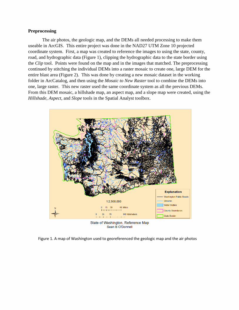
The air photos, the geologic map, and the DEMs all needed processing to make them useable in ArcGIS. This entire project was done in the NAD27 UTM Zone 10 projected coordinate system. First, a map was created to reference the images to using the state, county, road, and hydrographic data (Figure 1), clipping the hydrographic data to the state border using the Clip tool. Points were found on the map and in the images that matched. The preprocessing continued by stitching the individual DEMs into a raster mosaic to create one, large DEM for the entire blast area (Figure 2). This was done by creating a new mosaic dataset in the working folder in ArcCatalog, and then using the Mosaic to New Raster tool to combine the DEMs into one, large raster. This new raster used the same coordinate system as all the previous DEMs. From this DEM mosaic, a hillshade map, an aspect map, and a slope map were created, using the Hillshade, Aspect, and Slope tools in the Spatial Analyst toolbox.

Figure 1. A map of Washington used to georeferenced the geologic map and the air photos

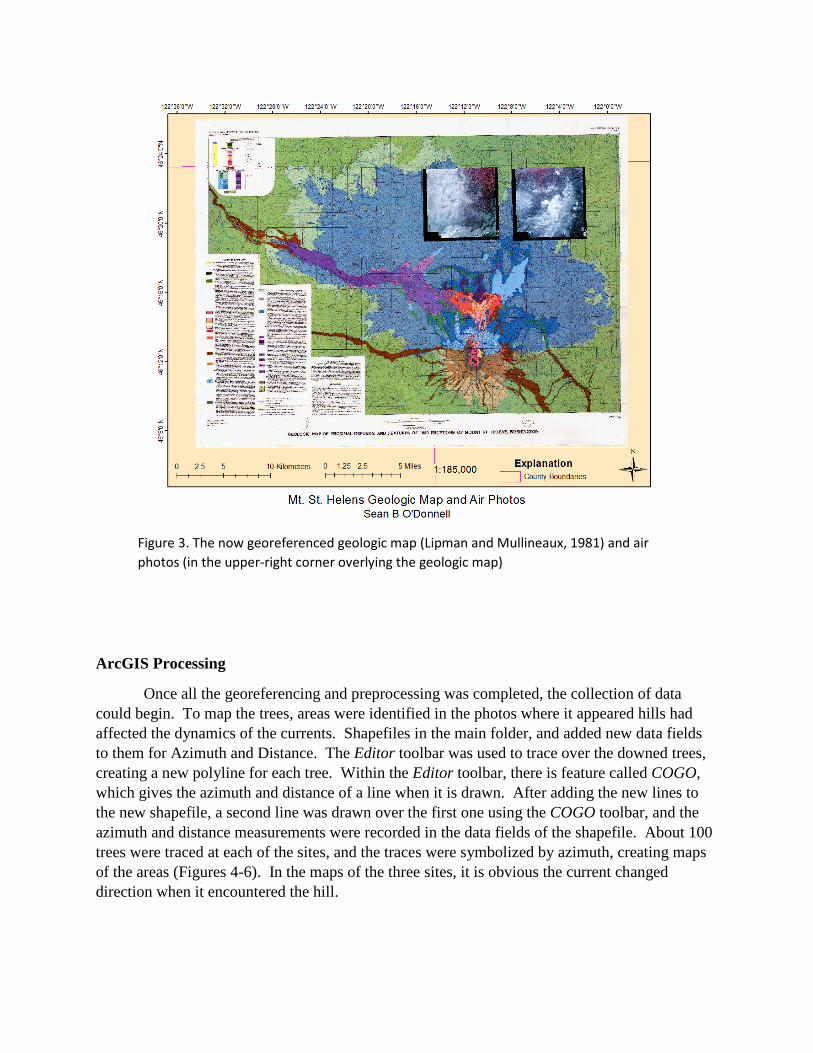
The air photos and geologic map were georeferenced using points that matched on the other spatially referenced files (Figure 3). This was done using the Georeferencing toolbar. Most of these points were county boundaries (for the geologic map only), lakes, and stream bends. Six reference points were selected on the geologic map and each of the three air photos to ensure that each image was properly referenced. Each image was also assigned the proper coordinate system in its Properties menu. Once the georeferencing was completed, the images were ready to be analyzed in ArcGIS.

Figure 2. A DEM of the Mt. St. Helens blast area. The high, large, blue, circular area in the bottom-right of the DEM is Mt. St. Helens. A Hillshade, Slope, and Aspect map were created from this raster.

ArcGIS Processing

Once all the georeferencing and preprocessing was completed, the collection of data could begin. To map the trees, areas were identified in the photos where it appeared hills had affected the dynamics of the currents. Shapefiles in the main folder, and added new data fields to them for Azimuth and Distance. The Editor toolbar was used to trace over the downed trees, creating a new polyline for each tree. Within the Editor toolbar, there is feature called COGO, which gives the azimuth and distance of a line when it is drawn. After adding the new lines to the new shapefile, a second line was drawn over the first one using the COGO toolbar, and the azimuth and distance measurements were recorded in the data fields of the shapefile. About 100 trees were traced at each of the sites, and the traces were symbolized by azimuth, creating maps of the areas (Figures 4-6). In the maps of the three sites, it is obvious the current changed direction when it encountered the hill.

Figure 3. The now georeferenced geologic map (Lipman and Mullineaux, 1981) and air photos (in the upper-right corner overlying the geologic map)

Points were created at the beginning of each of the lines using the Feature Vertices to Point tool. The azimuth, distance, aspect, slope, and elevation data was extracted from their respective files to these points using the Extract Multi-Values to Point tool, creating a large attribute table for these points. The attribute tables of these points were extracted to text files, and then to CSV files, to use and analyze in Excel.

Reference trees were measured to acquire a reference current direction to compare the direction of the current around the hills too. 16 reference trees were measured outside of the area impacted by the hill, and the azimuths averaged to create a reference azimuth.

Figures 4-6. Maps of the measured downed-trees around hills in the blow-down zone the PDCs. The colors represent azimuth, and there are burnt, standing trees in the center of the hills.

Results

The overall average data from all three sites is below in Table 2. The statistical measurements are taken from all 300 data points. The change in aspect represents the difference between the aspect at a point and the reference azimuth.

Azimuth Δ Azimuth Δ Aspect Mean 156.006 53.350 -108.071 Standard Deviation 135.394 68.896 117.447 Median 104.470 44.481 -123.193 Mode 315.000 82.050 38.050

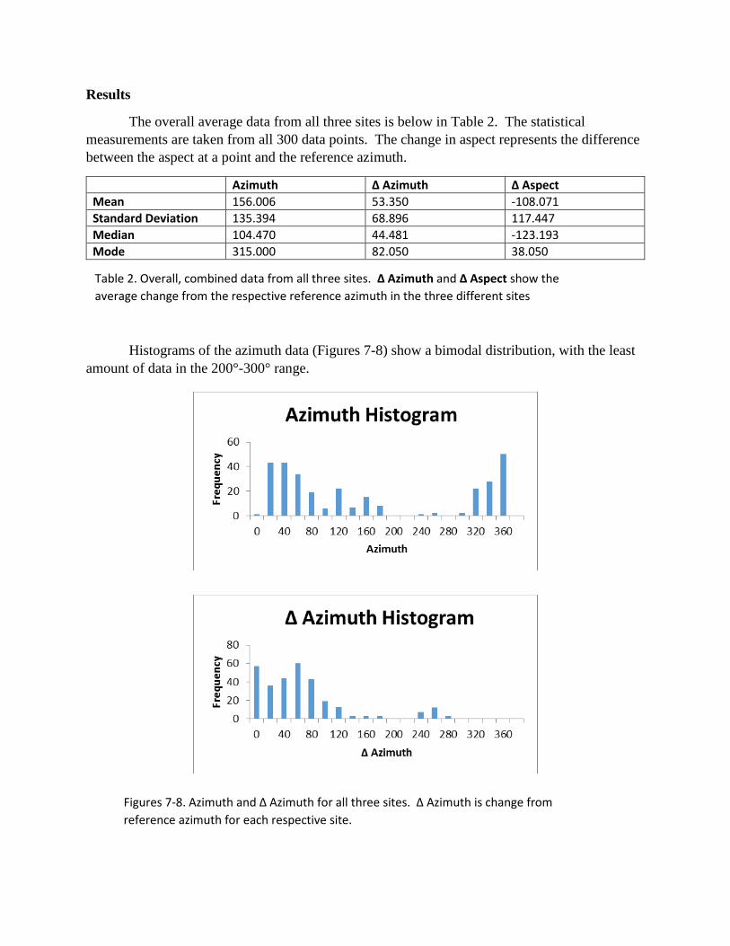
Histograms of the azimuth data (Figures 7-8) show a bimodal distribution, with the least amount of data in the 200°-300° range.

Table 2. Overall, combined data from all three sites. Δ Azimuth and Δ Aspect show the average change from the respective reference azimuth in the three different sites

Figures 7-8. Azimuth and Δ Azimuth for all three sites. Δ Azimuth is change from reference azimuth for each respective site.

Discussion

Azimuth and Δ Azimuth were compared to other sets of data to determine if there were any other controlling factors on current direction beside the hill itself. The azimuth was compared to slope at each point, aspect at each point, Δ aspect at each point, and elevation at each point. The results are shown in Figures 9-12.

Figures 9-10. Azimuth vs Slope and Aspect

There is very little to no correlation between Azimuth or Δ Azimuth and any of the other variables. The charts again do show the bimodal distribution of Azimuth, but not much of anything else. What this is showing then, is that when a current that is near buoyancy encounters an obstacle, such as a hill, it changes direction to get around the obstacle, but is not majorly affected by slope or aspect of the surrounding topography (a current not near buoyancy with a lot of momentum would just run over the hill). The controlling factor on the current dynamics is the hill itself, forcing the current to temporarily change direction to go around before continuing on its way beyond the hill. Eddies in the current also form in response to the hill and change in travel direction. Since the current does change direction, the direction of the blown-down trees

Figures 11-12. Azimuth vs Elevation and Δ Azimuth vs Δ Aspect

change with it and with any resultant eddies, but the direction the trees are blown down in is not majorly affected by the slope or aspect of the topography they are standing on before the current knocked them down.

Even though it appears that the current is controlled only by the obstacle in front of, and other major aspects of topography, there is still some more work that could be done in the future. Comparing the change in elevation from the top of the hill to the bottom, and the area in between to the blown-down trees may provide insight as to why the current when around the hill and did not jump it.