a probabilistic production simulation approach …
TRANSCRIPT

i
A PROBABILISTIC PRODUCTION SIMULATION APPROACH FOR
SYSTEMS WITH INTEGRATED CONCENTRATED SOLAR PLANTS
WITH THERMAL ENERGY STORAGE
BY
TI XU
THESIS
Submitted in partial fulfillment of the requirements
for the degree of Master of Science in Electrical and Computer Engineering
in the Graduate College of the
University of Illinois at Urbana-Champaign, 2015
Urbana, Illinois
Adviser:
Professor George Gross

ii
ABSTRACT
The global awareness of the impacts of climate change is a key driver of the quick pace
of development of renewable energy technologies. The concentrated solar plant (CSP)
technology has emerged as a promising approach to harness solar energy, with several
implementations under way around the world. Unlike PV and wind resources, a CSP
allows the deployment of the thermal energy storage (TES), which provides the CSP
operator the flexibility to produce electricity beyond the sunrise-to-sunset periods. For a
system with integrated CSPs at distinct locations on its footprint, the effective utilization of
the TES devices requires a scheduler to optimize the value of the total CSP-produced
energy for the system. However, the assessment of impacts of CSP resources poses major
challenges due to the inherent uncertainty, variability and intermittency of direct normal
irradiation (DNI), which markedly influence the times and the quantities of total CSP
energy production. The geographic correlations among the multi-site DNI and its intrinsic
seasonality further complicate the effective quantification of the multi-site CSP variable
effects in power systems into which they are integrated. Thus, the assessment of CSPs sets
up an acute need for a practical simulation approach to emulate operations of the systems
with integrated CSP resources and to evaluate their variable impacts. Such an approach
must explicitly represent the uncertainty, variability and intermittency of the CSP resources,
the geographic correlation among them, as well as the flexibility imparted by TES devices.
The approach also needs to take into account the seasonality of the CSP resources and their
interactions with the load seasonal changes.
To address these needs, we construct the multi-site CSP power output model and
formulate the associated scheduling problem (SP) under some specific TES operational

iii
objective in a system with integrated multi-site CSP resources. The power outputs of the
multi-site CSPs depend not only on the specific details of the CSP configurations and the
operational schedule, but also on the nature of the solar energy input. The identification of
distinct multi-site DNI data in a given season is a key step to obtain the analytic
representation of the multi-site CSP power outputs. We use statistical clustering techniques
to classify the distinct data into various groups – referred to as regimes – and utilize the
power output model to probabilistically characterize the multi-site CSP power outputs
based on the identified DNI regimes. We make detailed use of the conditional probability
concepts to incorporate the probabilistic model of the multi-site CSP power outputs into
the extended production simulation tool.
The major interest in the use of the extended production simulation approach is to
quantify the impacts of the integration of CSP resources into the system on the variable
effects over longer-term periods. We modify the Western Electricity Coordinating Council
(WECC) 240-bus model to construct a test system based on WECC geographic footprint,
using WECC historical load, DNI and system marginal price data. We present some
representative simulation results to provide insights into the multi-site CSP impacts on the
systems over longer-term periods and to illustrate the effectiveness of the extended
simulation approach.
The primary contribution of this thesis is to propose an approach capable of quantifying
the variable effects of the multi-site CSP resources on the system into which they are
integrated, with explicit representation of the uncertainty, variability and intermittency of
the solar resources as well as their interactions with the loads and other resources.

iv
For my family

v
ACKNOWLEDGMENTS
I would like to acknowledge the advice, guidance and support from my adviser,
Professor George Gross, throughout my courses and research at the University of Illinois. I
also thank Professor Peter W. Sauer, Professor Thomas J. Overbye and Professor Hao Zhu,
who gave me support on the completion of this thesis.
Special thanks to my dear friend, Chen Hu, with whom I spent a lot of time during the
past two years. I enjoyed his continuous presence and the moments when we worked,
studied and stayed together.
I would also like to thank all the power group students and staff for their help and
friendship. In particular, I enjoyed the wide range of the conversation topics with Kai,
Yannick, Mirat and Ada. We are always together fighting against challenges.
Finally, special thanks to my dear family without whom nothing is possible.

vi
TABLE OF CONTENTS 1. INTRODUCTION .......................................................................................................................... 1
1.1. Background and Motivation .................................................................................................... 1
1.2. Survey of the State of the Art .................................................................................................. 7
1.3. Scope and Contributions of the Thesis .................................................................................... 8
1.4. Outline of the Thesis Contents................................................................................................. 9
2. THE PROBABILISTIC MULTI-SITE CSP RESOURCE POWER OUTPUT MODEL ............ 11
2.1. The Deterministic Multi-site CSP Generation Model ........................................................... 11
2.2. The Multi-site DNI Model ..................................................................................................... 18
2.3. The Probabilistic Characterization of the CSP Power Outputs.............................................. 29
2.4. Summary ................................................................................................................................ 32
3. THE EXTENSION OF PROBABILISTIC SIMULATION APPROACH .................................. 33
3.1. Review of the Conventional Probabilistic Production Approach .......................................... 33
3.2. Reexamination of the Load Representation ........................................................................... 38
3.3. Extension of Production Simulation with Time-Dependent Resources................................. 41
3.4. Summary ................................................................................................................................ 42
4. ILLUSTRATIVE SIMULATION RESULTS .............................................................................. 43
4.1. The Test System and the Simulation Parameters ................................................................... 43
4.2. Study Set I: Impacts of the Deepening CSP Penetration ....................................................... 47
4.3. Study Set II: Sensitivity of the TES Capability ...................................................................... 52
4.4. Study Set III: Investigation of the Multi-site CSP Resource Ability to Replace Retired
Conventional Unit Capacity ......................................................................................................... 55
4.5. Study Set IV: Comparison of Two Different TES Operational Objective Impacts on the
Power Systems .............................................................................................................................. 57
4.6. Summary ................................................................................................................................ 59
5. CONCLUSION ............................................................................................................................. 61
5.1. Summary ................................................................................................................................ 61
5.2. Future Research ..................................................................................................................... 62
APPENDIX A: NOTATION ........................................................................................................... 63
APPENDIX B: THE SCALING ALGORITHM ............................................................................. 67
APPENDIX C: THE DESCALING ALGORITHM........................................................................ 69
REFERENCES ................................................................................................................................. 72

1
1. INTRODUCTION
In this thesis, we develop a probabilistic simulation approach for systems with integrated
concentrated solar plant (CSP) resources with thermal energy storage (TES) to evaluate the
impacts of the multi-site CSP integration on the system variable effects over longer-term
periods. In this introductory chapter, we present the background and motivation for this
research, briefly review the current state of the art, provide an overview of our proposed
methodology and outline the rest chapters of the thesis.
1.1. Background and Motivation
The growing concern over the impacts of global climate change has resulted in
legislation in numerous jurisdictions to encourage the implementation of renewable
resources for electricity supply so as to reduce fossil fuel energy dependence and to curtail
greenhouse gas emissions. For instance, more than half the U.S. states have set ambitious
goals through their Renewable Portfolio Standards specifying the percentage of the
electricity that needs to be served by renewable resources by specific target dates [1]. The
European Union has also established binding targets with the goal to derive 20 % of the
total European Union energy consumption from renewable energy sources by 2020 [2]. In
the solar energy technology arena, CSP technology has recently experienced a steady
growth, with nearly 11 GW of CSP projects under development around the world [3].
Typically, a CSP utilizes mirrors with tracking systems to focus direct normal irradiation
(DNI) to collect solar energy for conversion into thermal energy, which is used in a steam
turbine or heat engine that drives a generator to produce electricity [4]. Parabolic trough,

2
Solar tower, Dish stirling and Fresnel reflector are the four common forms of the CSP
technology [4]. Compared to the other two forms, parabolic trough and solar tower CSPs
are widely commercially deployed around the world [5]. The parabolic trough CSP
technology uses parabolic mirrors to concentrate solar rays onto the receivers positioned
along the mirrors’ focal line and the solar tower technology employs heliostats – flat
mirrors with dual-axis trackers – to focus DNI onto a central receiver [5]. Unlike PV
resources, CSP can make use only of the DNI – the direct component of the irradiation.
Furthermore, a salient characteristic of the CSP technology is the deployment of the TES to
store a fraction of the thermal energy for later conversion. Since the utilization of TES
allows CSP to produce electricity beyond the sunrise-to-sunset periods and to ensure that
the power outputs meet the forecasts with a better fidelity, the TES is a definite advantage
of CSP over the non-dispatchable PV resources. The added flexibility afforded by the TES
is a key reason for the growing interest in CSP [6], with the global installed capacity of
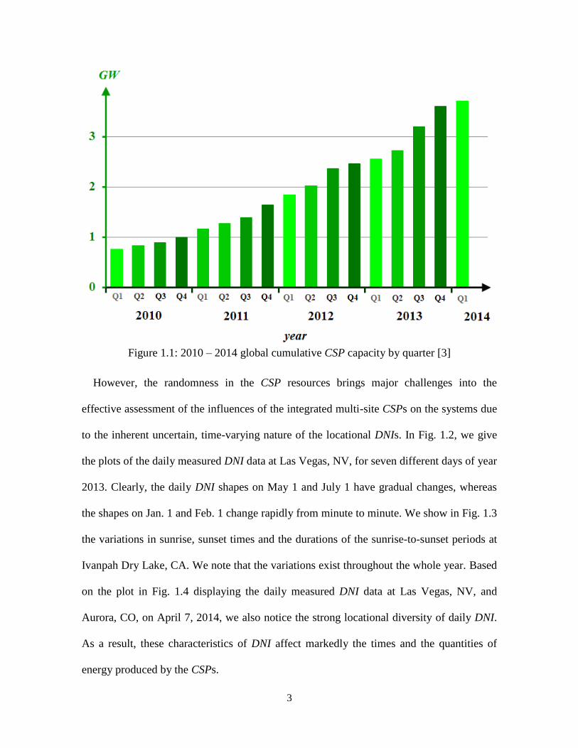
around 3,500 MW [3] by the end of 2013, shown in Fig. 1.1. Spain continued to lead the
world with the 2,304-MW total installed CSP capacity. The U.S. also installed 410 MW of
CSP in 2013, increasing its total CSP capacity by more than 80 %. Other countries
involved in wide commercialization of CSP resources include China, South Africa and
Australia. Therefore, the implementation of CSPs triggers an acute need for a simulation
tool to efficiently quantify, over longer-term periods, the variable effects of the power
systems with integrated CSP resources sited at distinct locations.
3
Figure 1.1: 2010 – 2014 global cumulative CSP capacity by quarter [3]
However, the randomness in the CSP resources brings major challenges into the
effective assessment of the influences of the integrated multi-site CSPs on the systems due
to the inherent uncertain, time-varying nature of the locational DNIs. In Fig. 1.2, we give
the plots of the daily measured DNI data at Las Vegas, NV, for seven different days of year
2013. Clearly, the daily DNI shapes on May 1 and July 1 have gradual changes, whereas
the shapes on Jan. 1 and Feb. 1 change rapidly from minute to minute. We show in Fig. 1.3
the variations in sunrise, sunset times and the durations of the sunrise-to-sunset periods at
Ivanpah Dry Lake, CA. We note that the variations exist throughout the whole year. Based
on the plot in Fig. 1.4 displaying the daily measured DNI data at Las Vegas, NV, and
Aurora, CO, on April 7, 2014, we also notice the strong locational diversity of daily DNI.
As a result, these characteristics of DNI affect markedly the times and the quantities of
energy produced by the CSPs.

4
Figure 1.2: Las Vegas daily DNI measurements for seven different days of year 2013 [7]
Figure 1.3: Ivanpah Dry Lake variations in sunrise/sunset times [8]

5
Figure 1.4: Las Vegas and Aurora daily DNI measurements on April 7, 2014 [3]
The CSP resources can output electricity whenever either solar energy or thermal energy
from TES is available. The efficient utilization of the TES requires a scheduler to optimize
the contribution of the CSPs to displace expensive and polluting conventional generation.
Thus, the extent to which the aggregated CSP energy production and the loads are
correlated is an important consideration in the evaluation of the multi-site CSP
contribution to the power systems. In contrast to the highly uncertain, variable and
intermittent CSP power outputs, the loads follow well-defined diurnal and weekly patterns
with higher demand during the weekdays than the weekends and with peaks, typically, at
similar periods of the weekdays and lower values at nights. We provide in Fig.1.5 the plots
of the hourly power outputs of the CSPs located in CAISO region in comparison with the
CAISO hourly loads [9] for March 10–16, 2014. The plots clearly indicate the weakly
correlated behavior of the CSP outputs with the loads, which considerably impacts the
multi-site CSP contribution to the power system where the CSPs are integrated. Due to the
seasonality of the DNI and the loads, such weak correlations are also strongly seasonally

6
dependent, which further complicates the assessment of the CSP contribution. Thus, the
proposed approach must be able to capture the time-varying nature of the CSP resources so
as to effectively quantify the variable effects of systems into which they are integrated.
Such a tool needs to explicitly represent the uncertainty sources in loads and resources, as
well as the interactions among them. It also needs to take into account the seasonality of
the loads and CSP resources, in addition to the TES operation scheduling and its impacts
on CSP outputs. In this thesis, we address those needs with the extension of the
conventional probabilistic simulation approach to construct a practical and versatile
simulation tool to emulate the operations of the power systems with integrated CSP
resources.
Figure 1.5: Plots of the chronological CAISO hourly loads and CSP power outputs for the
March 10–16, 2014 [9]

7
1.2. Survey of the State of the Art
The integration of the CSP resources into the electric grid has become increasingly
important in recent years with deepening CSP resource penetration. Here, we briefly
review the literature related to the issues we are dealing with in this thesis.
The modeling of the DNI and the CSP are the two key issues that need to be addressed
in the studies of systems with integrated CSP resources. The models’ complexity depends
on the nature of the study and the level of detail of the phenomena we want to capture. Due
to the time dependence of the earth’s and sun’s movements, the temporal effects are
always taken into account in the DNI modeling. For instance, the actual DNI value is
computed based on the clear-sky DNI value, which is determined by the time of the year,
and the atmospheric attenuation factor, which is approximated as a nonlinear function of
the geographical information [10]. For systems with dispersed CSP resources over a broad
area, the geographical correlations among the DNI also needs to be considered. In the solar
irradiation forecasting area, some computationally demanding methods are reported in [11],
[12] for PV resources. But those methods are only useful for short-term operational
decision and are inappropriate for longer-term planning.
Researchers have developed multiple models to emulate the behaviors of CSP resources.
Many of those techniques, described in [13], [14], [15], [16], focus on energy analysis and
consider only the energy production from the CSP resources without the evaluation of their
impacts on the system into which they are integrated. Although the methods in [17]
probabilistically represent the load, the controllable resources and the renewable energy
resources and the interplay among the resources and loads, the utilization of Monte Carlo
methods is computationally demanding to simulate larger power systems, and

8
modifications are required to simulate the operations of the systems with integrated CSP
resources. Several comprehensive studies have also studied the impacts of the wind and PV
resource integration for several U.S. systems [18], based on chronological production
simulations where the system operations are simulated step by step.
As a result, the electric power industry recognizes the need for new methods to
effectively assess the impacts of uncontrollable renewable energy sources [19] and is
intensified by the deepening renewable energy penetration.
1.3. Scope and Contributions of the Thesis
Little work has been done to construct a probabilistic simulation approach to emulate the
realistic power system operations with integrated multi-site CSP resources, particularly over
longer-term periods. The major challenge is to incorporate the additional uncertain and
time-varying effects of CSPs into the approach [20], [21]. Such an approach needs to take
into account the seasonality of loads and CSP resources, in addition to the TES operation
scheduling and its impacts on CSP outputs. It also needs to explicitly represent interactions
among loads and conventional controllable units. We address those needs to develop such
an approach in this thesis.
We extend the conventional probabilistic simulation tool to construct a practical and
versatile approach to effectively assess, over longer-term periods, the variable effects of
systems with integrated CSPs at different sites. We develop a multi-site CSP power output
model and formulate a TES scheduling problem (SP) to determine the daily multi-site CSP
power outputs using the given daily DNI values. For the effective use of the historical DNI
measurements to simulate the CSP power outputs, we introduce a common time scale to
9
allow the meaningful comparison of daily multi-site DNI data in a specific season and
deploy statistical clustering techniques to obtain an analytic characterization of the daily
multi-site DNI to construct the DNI regimes. We use the CSP power output model and the
regime-based DNI characterization to probabilistically represent the power outputs of CSPs
at distinct sites. We apply conditional probability concepts to incorporate the probabilistic
multi-site CSP power output representation into the extended probabilistic simulation
framework.
As such, the proposed methodology explicitly represents the uncertainty, variability and
intermittency of the CSP power outputs, the flexibility imparted by TES, as well as the
interactions among loads and resources. It also captures the seasonality of the loads and
CSP resources. The primary application of the extended approach is to evaluate the
contribution of integrated CSP resources to the power system over longer-term periods. We
illustrate the effectiveness of the proposed approach using representative results from the
extensive studies we performed on systems in different geographic regions under a wide
range of conditions. The studies we discuss provide a realistic assessment of the impacts of
the multi-site CSP resource integration on the systems’ reliability, economic and
environmental metrics.
1.4. Outline of the Thesis Contents
This thesis consists of four additional chapters. In Chapter 2, we focus on the
probabilistic characterization of the multi-site CSP resources for the simulation purposes.
We start with the modeling of the development of a deterministic model of the multi-site
CSP power output. Then, we focus on the DNI data processing for utilization to analytically

10
characterize the multi-site CSP resources. In Chapter 3, we briefly review the conventional
probabilistic production simulation tool and describe the steps to extend the production
simulation with integrated CSP resources. We describe the modified version of the WECC
test system in Chapter 4 and select some representative results from the extensive studies
we performed to illustrate the application of the extended probabilistic simulation approach.
We conclude our contributions and provide directions for future work in Chapter 5. There
are three appendixes at the end of the thesis. In Appendix A, we summarize the notations
used in this thesis. We describe in detail the scaling and descaling algorithms in Appendix
B and C, respectively.
11
2. THE PROBABILISTIC MULTI-SITE CSP RESOURCE
POWER OUTPUT MODEL
The quantification of the variable impacts, over longer-term periods, of the multi-site
CSP resources integrated into a power system requires the construction of a multi-site CSP
power output model, which explicitly represents the uncertainty, intermittency and
variability of the locational DNI and their impacts on the CSP outputs. We devote this
chapter to the description of the proposed multi-site CSP generation model and its
deployment to probabilistically characterize such outputs.
This chapter contains three sections. In Section 2.1, we derive a solution for an
optimization problem to determine the multi-site CSP power outputs, using the given DNI
values. In Section 2.2, we develop the probabilistic characterization of the locational DNIs
and introduce the notion of multi-site DNI regimes to explicitly represent the salient DNI
patterns in distinct geographical areas. We use the scaling algorithm to scale the historical
DNI data onto a common time scale so as to identify the days with similar scaled DNI
shapes. We introduce the descaling algorithm to convert the scaled DNI samples onto the
actual sunrise-to-sunset period of the day for simulation purposes. In Section 2.3, we
analytically characterize the multi-site CSP power outputs and describe the approximation
of the regime-conditioned distribution functions of the CSP power output random variables
(r.v.s). We use the notations defined in Appendix A.
2.1. The Deterministic Multi-site CSP Generation Model
We start this section with a brief description of the behavior of a stand-alone CSP. Many
conventional and nuclear power plants use heat to boil water to produce high-pressure

12
steam, which expands through the turbine to spin the generator rotor to produce electricity.
CSP technology extracts the heat from the solar energy and, in a way similar to the
conventional or nuclear plants, produces steam to generate electricity. A typical CSP set-up
includes four primary components: collectors that concentrate solar rays, receivers that
collect and convert solar energy into thermal energy, the TES that stores thermal energy for
later use, and a power block that converts thermal energy into electricity. We refer to the
collection of collectors and receivers as the solar field. We summarize in Fig. 2.1 the
energy flows in a typical CSP.
Figure 2.1: Energy flows in a typical CSP
For a power system with integrated CSPs at multiple locations, the power output of each
CSP depends on the DNI at its location, the specific CSP configuration and the utilization
schedule of the TES. The aggregated power produced by the CSPs must take into account
the correlations among the DNIs at the multiple locations. The CSP converts the solar
energy into thermal energy, used instantaneously either to generate electricity in the
turbines or to be stored in the TES for later conversion. The utilization of the TES allows

13
the CSP to produce electricity even outside the sunrise-to-sunset periods and to smooth the
total output of the CSP units. Moreover, the TES deployment enables the CSP operator to
construct a multi-site TES schedule to meet some specific operational objective, such as
the maximization of the total energy produced by the multi-site CSPs or the provision of a
smoothed, aggregated multi-site CSP power output. Such TES schedules lead to the inter-
temporal and spatial coupling of CSP operations at the different locations. We note that the
thermal energy can be charged into/discharged from the TES without the violation of each
TES’s maximum/minimum capability. The TES physical capability refers to the maximum
amount of thermal energy that can be stored in the TES. The storage hour capability is
expressed as the ratio of the physical capability to the maximum input of power block for
electricity generation [22]. The charging/discharging rate of each TES device must be
within its capacity range and the TES device operates at any point in time in only one of its
operational states – charge, discharge or idle. A TES device cannot charge and discharge
simultaneously. Typically, due to the nature of TES, the thermal energy also incurs losses
over time [23]. Such losses are specified either in terms of % or as a loss rate of energy in
units of MWh t /h.
We construct the power output model of a system with integrated CSPs at S sites to
emulate the multi-site CSP operations with TES for each day in a simulation period. For
simplicity, we assume that there is a single CSP at each site s. In the case of multiple CSPs
at a site s, we construct an equivalent single CSP to represent the aggregated individual
CSP outputs at the site. We decompose each day into H equal-duration sub-periods. We
assume that each variable of interest, except the value of stored energy, remains constant
during a sub-period. Since the energy storage is of critical interest, we adopt the

14
convention that we represent the value of each variable, including thermal energy stored, at
the end of each sub-period. The system loads and the DNI values for each sub-period are
assumed given. A sub-period is the smallest, indecomposable unit of time and determines
the resolution of the simulation. Any phenomenon of shorter duration than a sub-period
cannot be represented and so is ignored.
The instantaneous solar-to-thermal energy conversion at site s is given by the nonlinear
mapping ( )s , whose argument is the DNI d
s hu . Since the plant design of CSP is out of
the scope of the thesis, ( )s is not explicitly formulated in this work. We rely on the Solar
Advisor Model [22] – a dynamic model developed by NREL – to determine the amount of
thermal energy collected by the solar field in each sub-period for the geographic, weather
and time input data of the CSPs. The nonlinear mapping ( )s , whose argument is the
thermal energy d
s hz , is used to instantaneously convert the thermal energy into electricity:
4 3 2 1
,4 ,3 ,2 ,1 ,0
d d d d
s s s s
s s s s smax max max max
s s s s
dss s
h h h hh
z
z z z zz c
z z z
(2.1)
Here sc represents the site s CSP capacity, maxsz represents the thermal energy input rate
needed to guarantee that the site s power block produces electricity at its rated capacity and
,s i are function coefficients, i = 0, 1, …, 4 [22]. We utilize the TES status variables d
s hv ,
d
s h {0,1} to define the operational state of a TES device. d
s hv ( d
s h ) is equal to 1
when the TES charges (discharges). Both are 0 when the TES device is idle. ds h denotes
the stored thermal energy at the end of the sub-period h. We represent the TES charging

15
(discharging) efficiency by the constant s (
s ) (0,1] . We also denote the thermal
energy loss rate, expressed in units of percent per sub-period, by the constant s
ψ . The TES
physical and operational capability limits are given by mins and max
s * . The sub-period
charging (discharging) rate d
s hk ( d
s hq ) has values within its allowed min max
s s,k k
(min max
s s,q q ) range.
We formulate the scheduling problem (SP) [13], [14], [22], [23], [24], [25], to
determine the optimal day d operational trajectory of each CSP with TES, using the hourly
DNI values in the array 1 2
d d d
S ... u u u . The SP is formulated as a constrained
optimization problem. The set of constraints comes from the TES physical characteristics
and operational limits. For the specified TES objective function, each coefficient d
sh
can be determined either from historical data or from forecasts or be some given values.
The detailed statement of the daily SP for day d is:
1 1
{
, 1,2,..., , 1,2,... }
(2.2 )d d d d ds s s s s
d ds s
H Sd d
s s
h sk h ,v h ,q h , h , h ,
hz p, h h H s S
h h max p a
subject to
* The physical capability
maxs , expressed in the units of MWht, refers to the maximum amount of stored
thermal energy; the storage capability is expressed as the ratio of the physical capability to maximum input of
power block for electricity generation. The TES capability, expressed in hour units, is the ratio of maxs to
max
sz .

16
1(1 )
1
s
d d d d
s s s s s s H
d d
s s
d d d d
s s s s s
d d
s s s
min d max
s s s
min d max
s s s
d min d d max
s s s s s
d min d d max
s s s s s
d
s
h h h h
h h
h h h h
h h
h
h
h h h
h h h
ψ k q
v
z u k q
p z
z z z
v k k v k
q q q
v
(2.2 )
(2.2 )
(2.2 )
(2.2 )
1 2 ...
(2.2 )
1 2 ...
(2.2 )
(2.2 )
(2.2 )
{0 1} (2.2 )d
s
, , ,
, , ,
, ,h h
b
c
d
e
h = H
f
s = S
g
h
i
j
For the given DNI values, the solution of the deterministic SP in (2.2) determines the
optimal multi-site CSP operations and power outputs for each sub-period of day d. Without
TES, no scheduler is needed since all the thermal energy is instantaneously converted to
electricity with
d d
s s s s = h hp u (2.3)
To illustrate the application of SP in our work, we provide in Figure 2.2 the plots of the
hourly power outputs for day 180 of year 2007 of a CSP located at Midland, Texas,
without/with a TES device. The CSP parameters are: 0 95s s . , 0.03sψ , 0min
s ,
t840 MWhmaxs 0 or , t50 MWmin
sz , t140 MWmax
sz ,min max min max
s s s s, ,k k q q
t0,140 MW , 60MWsc and ,4 ,3 ,2 ,1, , , ,s s s s ,0 0, 0, 0, 0, 0.3s . Each

17
objective function coefficient is set to 1.
(a) without TES
(b) with 6-hour TES
Figure 2.2: The CSP power outputs without TES in (a) and with 6-hour TES in (b) for day
180 DNI (dotted line) in year 2007 at Midland, Texas

18
As shown in Fig.2.2 (a), the CSP energy production at each hour without TES is totally
determined by its hourly DNI value. When the DNI value is low, the CSP power output is
low, and when the DNI value is high, the CSP power output is high but cannot violate its
capacity. In Fig.2.2 (b), the TES stores thermal energy for electricity production and
mitigates the impacts of DNI intermittency on the CSP energy production. The two plots
in this example illustrated the capability of SP formulation to emulate the behavior of CSP
resource without and with TES.
The SP forms the basis to characterize the multi-site CSP power outputs. However, for
each day d, the locational DNI values are highly uncertain and so we represent them as the
realizations of the DNI random variables (r.v.s) at the S sites. The historical data
1 2
d d d
S ... u u u are indeed the measured values of these r.v.s. As such, the SP solution
maps these DNI realizations into the realizations of the power output r.v.s.
1 2
d d d
S ... p p p . In this way, we probabilistically characterize the multi-site CSP
power outputs.
2.2. The Multi-site DNI Model
As the first step in the probabilistic characterization of the CSP power outputs, we analyze
the multi-site DNI data obtained from the measurements at the S sites. A single
measurement is used in each sub-period at each site. We assume that these measurements
are made simultaneously at all the S sites in each sub-period during each site’s sunrise-to-
sunset period. For a probabilistic characterization, we use as many data points as we can
collect. However, the analysis of these data is complicated by the variations in the sunrise-

19
to-sunset periods at the S sites. We consider a data set of I days in a given season, with
possibly several years of data collected. The date of each day i in the data collection is
known, as are the corresponding sunrise and sunset times at each site s. From the i
sM DNI
measurements ˆ i
s mu taken at equal intervals during the sunrise-to-sunset period in day i,
we construct the corresponding DNI measurement vector :
1ˆ
ˆ ˆ
ˆ
is
i
s
Mi i
s s
i
sis
m
M
u
u
u
u (2.4)
To allow the effective comparisons of the DNI data from different days of a season, we
introduce a scaling scheme over the sunrise-to-sunset period of each day into the common
time scale with J equal-duration time-scaled sub-periods. The scaling process maps the
measurement elements in ˆ i
su into the computed vector i J
s y on the common time scale.
Mathematically, we represent the scaling process as the transformation from isM into J
and express it as:
1
ˆ( )
i
s
i i i Jis s s s
i
s
j
J
y
y
y
y u (2.5)
We visualize the time scaling process as shown in Fig. 2.3.

20
Figure 2.3: The time scaling process in day i at the S sites produces the computed DNI
values for J equal time-scaled sub-periods from sunrise to sunset
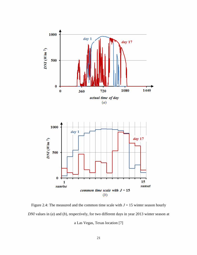
We provide in Fig. 2.4 an illustrative example of the application of this scaling process to
the single Las Vegas, Texas, DNI shapes for year 2013. The detailed steps of scaling
algorithm are discussed in Appendix B in [26].
We continue with the discussion on the use of the common-time-scaled computed
variables i
sy . For each day i, we construct the scaled DNI array
1 2
i i i i S
S
J ... Y y y y (2.6)
using the S vectors i
sy , s = 1, 2, …, S. iY represents realizations of the daily multi-site
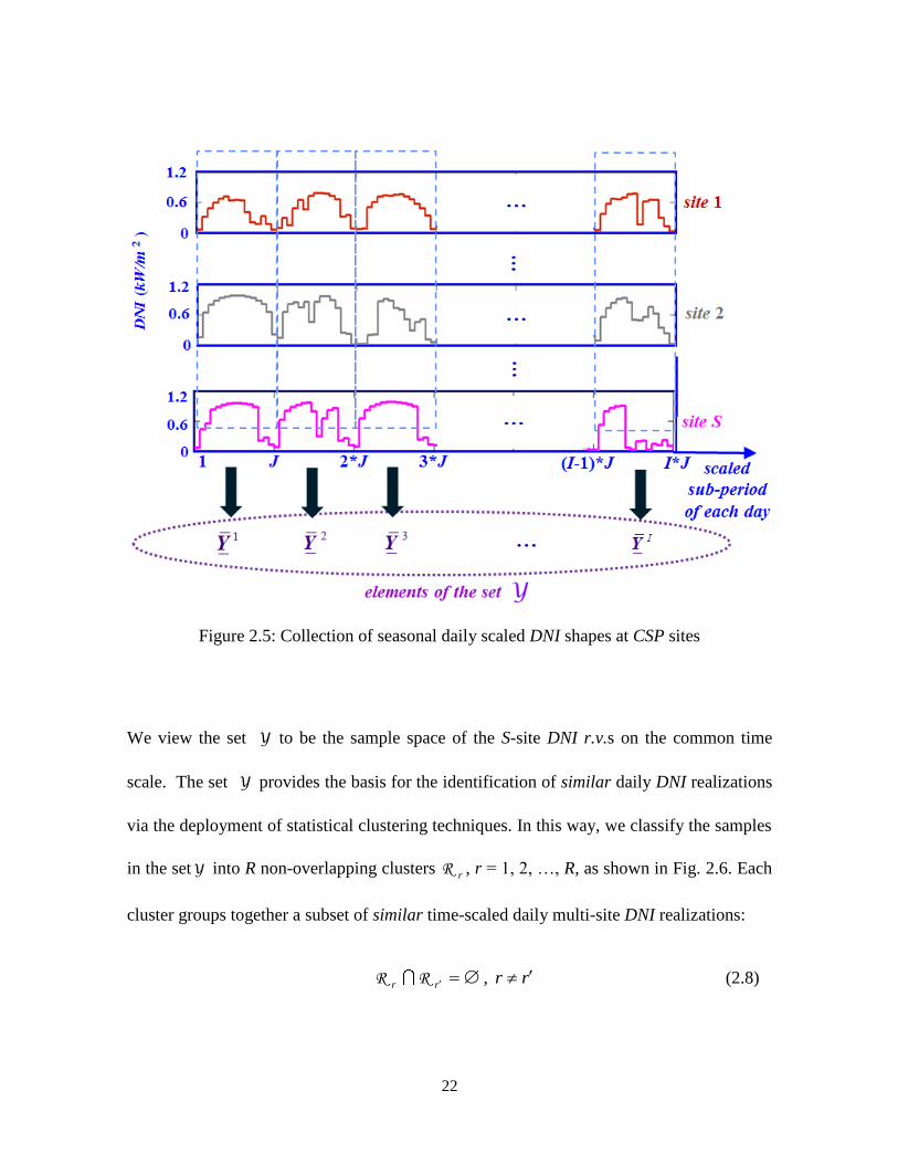
DNI on the common time scale at the S sites. As shown in Figure 2.5, we collect arrays
iY for I days and construct the set
= { : 1, 2, }i i ... , IYY (2.7)
21
Figure 2.4: The measured and the common time scale with J = 15 winter season hourly
DNI values in (a) and (b), respectively, for two different days in year 2013 winter season at
a Las Vegas, Texas location [7]
22
Figure 2.5: Collection of seasonal daily scaled DNI shapes at CSP sites
We view the set Y to be the sample space of the S-site DNI r.v.s on the common time
scale. The set Y provides the basis for the identification of similar daily DNI realizations
via the deployment of statistical clustering techniques. In this way, we classify the samples
in the setY into R non-overlapping clusters rR , r = 1, 2, …, R, as shown in Fig. 2.6. Each
cluster groups together a subset of similar time-scaled daily multi-site DNI realizations:
r r R R , r r (2.8)
23
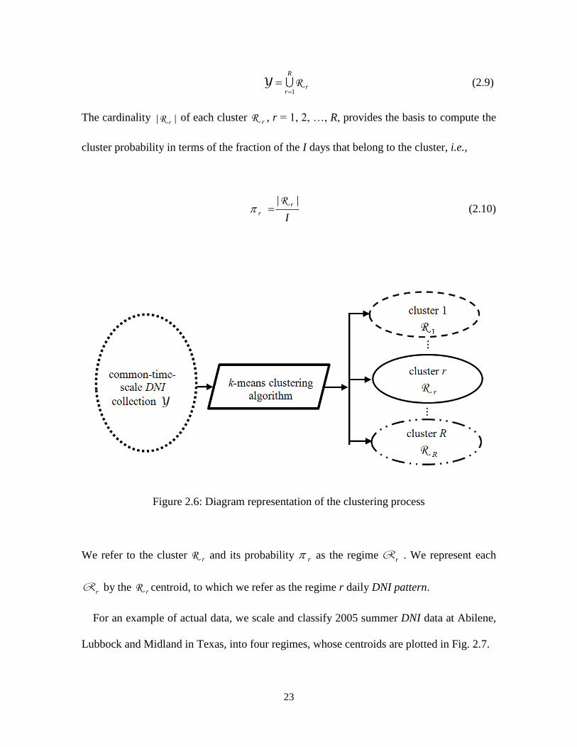
1
R
rr
Y R (2.9)
The cardinality | |rR of each cluster r
R , r = 1, 2, …, R, provides the basis to compute the
cluster probability in terms of the fraction of the I days that belong to the cluster, i.e.,
| |r
rI
R
(2.10)
Figure 2.6: Diagram representation of the clustering process
We refer to the cluster rR and its probability r as the regime
rR . We represent each
rR by the r
R centroid, to which we refer as the regime r daily DNI pattern.
For an example of actual data, we scale and classify 2005 summer DNI data at Abilene,
Lubbock and Midland in Texas, into four regimes, whose centroids are plotted in Fig. 2.7.

24
Figure 2.7: The centroids of the common-time-scale computed values of the four DNI
regimes with J = 80, obtained via the k-means clustering algorithm [27], for the summer
DNI data at the three Texas sites – Abilene, Lubbock and Midland
prob: 0.49 prob: 0.23
prob: 0.17 prob: 0.11

25
Figure 2.8: The representation of the sampling of the physical measurements and the
descaling process for the computation of the day d data at the S CSP sites
We make effective use of conditional probability to probabilistically characterize the
multi-site CSP resources in terms of the R regime representation [28]. We draw random
samples from each cluster rR to use as inputs into the multi-site CSP power output model.
The simulation of a specified day d in the given season requires that a sample be
appropriately descaled into the day d multi-site sunrise-to-sunset periods. We descale the J
DNI values at each site s in the drawn common time scale sample into the computed DNI
values 1T
d d ,b d d ,b d d ,e
s s s s s sh h hu , u , ... , u for the ( 1d ,e d ,b
s sh h ) equal-duration
sub-periods in the day d sunrise-to-sunset period at each site s. We represent the descaling

26
process by the transformation d
s . We summarize in Fig. 2.8 the sampling and descaling
step.
To maintain consistency of the midnight-to-midnight representation of the loads, we use
the components of the descaled vector 1T
d d ,b d d ,b d d ,e
s s s s s sh h hu , u , ... , u to
construct the augmented daily vector for the entire H-sub-period day with
1d
s
d d ,b
s s
d H
s
d d , e
s s
d
s
h
h
H
u
u
u
u
u (2.11)
where d
su represents the day d site s DNI realizations from midnight to midnight, with:
0ds hu for , ,[1 1] [ 1 ]d ,b d ,e
s sh h h H (2.12)
To illustrate the descaling and the augmented vector construction, we provide in Figure 2.9
the plots of the common time scale DNI data and the daily descaled DNI for day 165 of
year 2013 at Austin, Texas. The vector d
su is simply a realization of the r.v. vector:
1d
s
d Hds s
d
s
h
H
U
U
U
U (2.13)

27
Figure 2.9: The common time scale with J = 20 values of a sample we used to construct the
DNI vector for day 165 of year 2013 at Austin, Texas in (a) with the corresponding values
of the daily descaled DNI vector (H = 24) in (b) [7]

28
We denote the realization of the r.v. vector d
sU conditioned on the cluster rR , i.e., d
s rU ,
by the augmented vector d
s ru . We construct the DNI r.v. array d
U from the S vectors:
1 2
d d d d
S
H S ...
U U U U (2.14)
and the corresponding DNI r.v array conditioned on cluster r
R :
1 2
d d d d
Sr r
H S
r r ...
U U U U (2.15)
For given DNI values, the solution of the SP that maximizes the objective function in
(2.2a) in (2.2) is the optimal multi-site CSP power outputs at the S sites. In particular, for a
given sample of conditioned multi-site DNI r.v.s – 1
d
rU , 2
d
rU , …,
d
Sr
U , the solution
obtained the corresponding optimal sample of conditioned multi-site CSP power output
r.v.s – 1
d
rP , 2
d
rP , …,
d
Sr
P , which are conditioned on cluster rR . We depict the
mapping process in Figure 2.10 to indicate that the deterministic SP solution maps each
sample into the conditioned optimal outputs. In this way, we obtain the multi-site CSP
power output r.v. sample space, which we can deploy to approximate the multi-site CSP
resource power output r.v.s cumulative distribution function (c.d.f.).
Thus, the SP together with multi-site DNI clusters provides the probabilistic
characterization the multi-site CSP resource power output r.v.s . We devote the next
section to the probabilistic characterizations of the CSP power outputs based on SP and the
multi-site DNI model.

29
Figure 2.10: Mapping from the multi-site DNI r.v. sample space into the multi-site CSP
power output r.v. sample space using the SP
2.3. The Probabilistic Characterization of the CSP Power Outputs
The regime-based DNI model provides the basis to construct the probabilistic model of
the CSP power outputs. The SP solution for each input DNI sample drawn from a cluster
rR determines the corresponding conditioned CSP power output realization. We represent
such a conditioned realization by the array d
rP :
1 2
d d d d
Sr r r r
H S...
P p p p (2.16)
Mathematically, d
rP is the corresponding realization of the multi-site CSP power output
r.v. array dP conditioned on cluster r
R , where:

30
1 2
d d d d
Sr r
H S
r r...
P P P P (2.17)
The computation of the day d multi-site CSP power output requires that we sample from
each cluster r
R , r = 1, 2, …, R, and determine the corresponding conditioned realization
of d
rP . We use the conditioned realization of the power output for each sample drawn
from a cluster rR to construct the subspace of the sample space of d
P , with multiple
samples from that particular cluster rR . We systematically repeat such a procedure for
each regime r
R and obtain the R subspaces for each conditioned d
rP , r = 1, 2, …, R.
The sample space of dP is simply the union of the non-overlapping subspaces that we
construct for the repeated sampling from the R clusters.
We compute the total aggregated conditioned power outputs of the CSPs at the S sites
for each sub-period h to be:
, 1
Sd d d
sh r r rs=
h hp p p
(2.18)
We then construct the daily power output vectors:
1
Sd d
s rr s=
p p (2.19)
For each sub-period h, we approximate the c.d.f. ( )d
h , rP
F
and its moments by using the
sample space of d
rP . In terms of the conditional probabilities, we state the c.d.f.

31
( )d
hP
F
to be:
1
1
( )
{ }
= ( )
{ }
= { }
= { }
(2.20)
d
h
d
h , r
r
r
d
P h
d
r h
Rd
r h , r
R
rP
x x
x on each
Pro
x
b
Prob
Prob Pr
x
ob
F
F = P
P
P
R
R
Also, for the day d, we approximate the joint c.d.f. ( ... )
r
d F , , ,
P
for the H hourly values
of d
rP – the sum of the conditioned r.v.s.
1
d
rP ,
2
d
rP , …, d
S rP , which we use to
compute the ( ... )
r
d F , , ,
P
with
1
1 2
1 2
( ... )
= ( ... )
1, 2, ...
{ }
(2.21)
d
d
rr
d
H h h
R
H r
x x x Prob x
x
h
x x
F , , , = P , ,H
F , , ,
P
P
The probabilistic characterization of the multi-site CSP resource power outputs in (2.16)
– (2.21) is the foundation of the extension of the conventional probabilistic production
simulation approach to represent the multi-site CSP power outputs in a system with
integrated CSPs.
32
2.4. Summary
This chapter provides a description of the construction of a probabilistic model for the
multi-site CSP resource power outputs, using sets of seasonal DNI data at the S sites with
CSPs. We first formulate an optimization problem used to compute the multi-site CSP
power outputs. Then we scale the seasonal daily DNI data into a common time scale so
that we are able to compare the data of different days in a meaningful way. We classify the
time-scaled DNI data into several clusters. For simulation purposes, we de-scale the
samples drawn from each cluster and use them to compute the corresponding multi-site
CSP power outputs for the day of interest. We use these samples to approximate the
conditional distributions of the CSP output random variables.
In the next chapter, we provide a brief review of the conventional probabilistic
production simulation approach and describe the steps needed to incorporate the multi-site
CSP output model into the probabilistic production simulation framework.

33
3. THE EXTENSION OF PROBABILISTIC SIMULATION
APPROACH
The probabilistic simulation approach is widely deployed in the evaluation of the
expected energy production by each unit over a specified study period, the reliability
metrics, the expected system production costs, the expected greenhouse gas emissions and
any other metric of interest to measure the variable effects. The conventional probabilistic
simulation is a computer-based emulation of the power system supply- and demand-side
resource operations to assess how effectively the demand is met over a specified period.
However, the conventional approach cannot represent time-varying resources such as CSPs.
In this chapter, we review the probabilistic production simulation tool basics and discuss
the necessary modifications to incorporate the model developed in chapter 2 to represent
the integrated multi-site CSP resources. We also discuss some implementation aspects of
the extended simulation approach.
3.1. Review of the Conventional Probabilistic Production Approach
To realistically emulate the operation of a power system, we decompose a multiple-year
study horizon into W non-overlapping simulation periods. We specify each simulation
period in such a way that no changes in the resource mix, unit commitment and the policy
environment occur during its duration. Such changes may occur, however, in subsequent
periods. We denote the index set of sub-periods in each simulation period by T :
={1, 2, ..., }TT (3.1)

34
For concreteness in this description, we choose a week as the simulation period and one
hour as the smallest, indecomposable unit of time with T = 168 and H = 24. We illustrate
the general structure of our scheme in Fig. 3.1. We note that the structure of the scheme is
sufficiently general to accommodate any desired granularity.†
Figure 3.1: The general structure of the scheme based on the partitioning of the study
period into W simulation periods, with each simulation period partitioned into T simulation
sub-periods and each sub-period equal to the smallest, indecomposable unit of time
The load and resource characteristics, as well as the unit commitment in each simulation
period are inputs into the simulation. Based on the chronological load data for the given
simulation period, we develop a probability distribution to represent the load r.v. L . To do
so, we ignore the time information and rearrange the loads in order of decreasing values
from the highest to the lowest and construct the load duration curve (l.d.c.). The reordered
load values contain no temporal information and all the inter-temporal effects are also lost
in this representation. As an example, we plot in Fig. 3.2 the ERCOT chronological load
data for Monday, July 25, to Sunday, July 31, 2011. We display in Fig. 3.3 the
† With the consideration of the thermal dynamic process, we adopt the granularity no less than 15 minutes as
one sub-period. If, however, granularity smaller than 15 minutes is chosen for the simulation, the
modifications of the SP are needed to take into account the dynamics of the thermal processes.

35
corresponding l.d.c.. We can identify the maximum/minimum load values from the l.d.c.
during the simulation period. We interpret the l.d.c. as the complement of the c.d.f. of L .
Consider an arbitrary point ( , h ) on the l.d.c.. We also interpret such a point as the
statement that the load exceeds the value of for h hours during the T hours of the
simulation period. The normalization of the time provides the fraction h/T, which we view
to be the probability that the load exceeds the value in the simulation period. Thus, we
use the inverted l.d.c. L to analytically characterize c.d.f. ( )LF of L :
( ) ( ) 1 ( ) 1 ( ) LProb L Prob L F L (3.2)
Figure 3.2: The ERCOT system chronological hourly load from Monday, July 25, to
Sunday, July 31, 2011 [18]

36
Figure 3.3: The l.d.c. for Monday, July 25, to Sunday, July 31, 2011.
A unit generates energy to serve the load, once it is committed and dispatched [29]. In
each simulation period w, wE is the index set of the committed conventional units and can
be viewed as a subset of the E – the set of conventional generation units, where:
={ , 1, 2, ..., }i i E E| | (3.3a)
={ :1 and unit is committed in simulation period }w i i i w E E| | (3.3b)
We model the availability of each controllable unit by its multi-state available capacity r.v.
[29]. Each unit may be represented by a single-block or a multi-block model. The blocks of
the committed units in wE are loaded to meet the load in the order of their non-decreasing
marginal prices during the period w. In this way, we construct the period w loading order

37
of committed units and we refer to this order as the loading list. The probabilistic
simulation approach uses the notion of the equivalent load r.v. kL – the remaining
uncertain load served by the blocks in the loading list after the first 1k blocks are loaded.
The recursive relation
1 0k k k with =L L A L L (3.4)
computes the equivalent load r.v. kL iteratively, where kA represents the available
capacity r.v. of the loading block k. We assume that each unit is independent of each other
unit and the load, and compute the 1 L , 2
L , … functional values rapidly by convolution
to evaluate the variable effects of the power system in each simulation period. Here, kL is
the inverted l.d.c. corresponding to the equivalent load r.v. kL . As an example, we use
1 kL to determine the expected energy production k of loading block k over the
simulation period:
1
1( )
k
k
k
C
k
C
d
L (3.5)
with
1
1, 2, ...k
k q
q
C c k
(3.6)
where qc is the capacity of the block q.
Given the heat rate and fossil fuel data for each loading block q, we can compute the
block k expected production costs and emissions during the simulation period. In addition,

38
the production simulation also provides, as a byproduct, the values of the system reliability
metrics of interest. Since the l.d.c. of the equivalent load r.v. after all the blocks are loaded
provides the complement of the c.d.f. of the load that remains unserved, we can derive the
relations to determine the loss of load probability (LOLP w) and the expected unserved
energy (EUE w) by:
w w
w
K KLOLP CL (3.7)
( )w
wK
w
K
C
EUE d
L (3.8)
where K w is the number of blocks loaded during the simulation period w. We make use of
(3.7) and (3.8) in the evaluation of the metrics of interest.
3.2. Reexamination of the Load Representation
To mesh the probabilistic simulation framework with the probabilistic model of the
multi-site CSP power outputs, we need to reexamine the load sample space. In each weekly
simulation period, we collect the H daily load values to construct the load r.v. sample
space of the T load values, where T is the total number of sub-periods in the simulation
period. We use the aggregated CSP power output r.v. d
hP
in each sub-period h to meet
part of the corresponding load of the sub-period. To do so, we partition the load r.v. sample
space into H non-overlapping subsets, with each subset containing realizations of the load
r.v. conditioned on the sub-period h. Consequently, we may view the sample space as a
39
matrix with D rows and H columns. Let 1 2, , ... ,
HT T T be the H subsets of
T , with
each subset h
T being a subset of the indices, one for each day, of the sub-period h for
the D days in the simulation period w . Thus, we write
1
H
hh
T T (3.9)
h h
for h h
T T (3.10)
Figure 3.4: The load representation for the partitioned r.v. sample
We use the samples in the set { , }j hjT to approximate the c.d.f. ( )
hL
F of the load
r.v. conditioned on the sub-period h. We summarize in Fig. 3.4 the visualization of the

40
load r.v. sample space partition we use in this analysis. Since each of the H non-
overlapping subsets has an equal probability 1/H, the application of conditional probability
allows us to restate the c.d.f. ( )LF of L in terms of the conditioned c.d.f.s of h
L . Thus,
1
1
( ) { }
= { }
= { } { }
1= ( ) (3.11)
|
L
H
h
H
L hh
in each sub - period h
hour h h
F = Prob L
Prob L
Pro our hb L Prob
FH
Under the assumption that each unit has uniform characteristics during the entire
simulation period, we express the c.d.f. ( ) k
LF of the equivalent load r.v. k
L similarly in
terms of the conditioned c.d.f.s of k
hL . In this way,
1
1( ) { }= ( )
k hk
H
L k L h
F = Prob L FH
(3.12)
where ( )k h
L
F denotes the probability of the equivalent load r.v. conditioned on the sub-
period h. We restate all the probabilistic simulation relations in terms of the conditional
probability with the conditioning on the sub-period h of each day in the simulation period.

41
3.3. Extension of Production Simulation with Time-Dependent Resources
We incorporate the representation of the multi-site CSP resource impacts by making use
of the load sample space partitioning in combination with the regime-based multi-site CSP
power outputs. The multi-site CSP power output r.v. meets some of the demand, with the
conventional controllable resources serving the other part. We use the term “controllable
load” C to represent the remaining “net” load r.v. that is met by the conventional units,
explicitly taking into account the output provided by the CSPs. We use the conventional
assumption that the load and multi-site CSP power output r.v.s are statistically independent.
We approximate the c.d.f. ,
( )C
h rF of the controllable load r.v. conditioned on the cluster
rR for the sub-period h making repeated use of the convolution operation. We then restate
the c.d.f. ,
( )C
h rF of the controllable load r.v. conditioned on the cluster r
R as:
1,
|1
{ }( ) = ( ) h
H
rC C r h r
Prc cobF = FcCH
R (3.13)
Once the approximation of ( )C
rF for a regime r is obtained, the probabilistic simulation
for the controllable resources proceeds exactly as under the conventional case. The
expected value of each metric of interest in a simulation period is evaluated as the cluster-
probability-weighted average of the conditional expected values.
For the entire study period, the expected value of each metric, such as a reliability index,
an economic measure or an environmental emission value, is computed as the sum of the
expected values in each simulation period.

42
3.4. Summary
In this chapter, we present a review of the probabilistic production simulation
framework for systems whose resource mix is constituted only of controllable units. We
devote the rest of this chapter to discuss the extension of its capability to explicitly include
the representation of CSP resources. We modify the load representation so that it is
compatible with the regimes-based CSP power probabilistic representation developed in
Chapter 2. In the next chapter, we discuss the application of the extended probabilistic
simulation approach to assess the variable effects of systems with integrated CSP resources.
43
4. ILLUSTRATIVE SIMULATION RESULTS
The extended probabilistic approach has a wide range of applications, including resource
planning, production costing issues, environmental assessments, reliability and policy
analysis. We carried out extensive simulation studies with the extended probabilistic
approach and devote this chapter to presenting representative results that illustrate the
capabilities of the approach to quantify the variable effects of a system with integrated
multi-site CSP resources. We start out with a description of the test system characteristics
used in the representative studies discussed here. We present the results of the four study
sets selected for the discussion in this chapter. In the study set I, we focus on the
investigation of the impacts of deepening CSP penetration. We discuss the impacts of the
TES capability in the study set II. The study set III results provide insights into the
capability of the multi-site CSPs to replace the retired conventional generation capacity.
We analyze the impacts of two different TES operational objectives on the simulation
results for the study set IV.
4.1. The Test System and the Simulation Parameters
We use a single test system for the four study sets reported in this chapter. In our
discussion, each simulation study is considered for the year 2004 so as to focus on the
nature of the results and the insights they provide. The test system is a modified version of
WECC 240-bus system [30]. The test system represents only the resources and loads
without the network. We scale the 2004 WECC load data so that the annual peak load is
81,731 MW. The test system has 902 conventional generation units with a total nameplate
capacity of 96,443 MW and we explicitly represent the unit maintenance schedule. The
44
reserves are maintained at 15 % level throughout the year. We use the outage probability
and the economics of every block for each conventional unit from [30]. The fuel costs and
CO 2 emission rate data are also those given in [30]. Each case study considers CSPs with
equal capacity installed at six selected sites. The six sites selected for the CSPs are all on
the WECC footprint, namely Barstow, Blythe and Lancaster in California, Lovelock and
Mercury in Nevada, and Tucson in Arizona. Each CSP uses the parabolic trough structure
with a solar multiple of 2. We use historical DNI measurement data with M = 24 from
2002 – 2004 [31] to identify the DNI clusters for our studies. We assume that each TES is
operated to maximize the total energy production of the aggregated CSP units. For the SP
objective function, each coefficient d
s h is assumed to be 1.
We partition the 52 weeks of the study year into four seasons and use one hour as the
smallest indecomposable unit of time for each day with H = 24. Given the importance of
the J value in the DNI pattern representation, the J choice involves a trade-off between the
accuracy of the solar pattern representation and the computational burden. We determine
the J value from a sensitivity study over the [0,100] interval. For each value of J, we scale
and then descale DNI data and evaluate the average absolute difference between the
descaled DNI data and its measured value expressed in per unit of the measured DNI value.
For the specified M and H values, we plot in Fig. 4.1 the average error for the range of
study for J. As J increases, the average error decreases. In our simulations, we use J = 80
to obtain an average error at or below 1 % level for the equal-duration common time-
scaled sub-periods in the CSP model.

45
Figure 4.1: The average error as a function of J
Figure 4.2: The centroids (J = 80) of DNI regimes for R = 3, using k-means clustering
algorithm for the autumn season at the six sites selected for simulation
An important parameter to be determined is the number of regimes to use in the DNI
representation. To gain some insights into the value of R, we scale the 2002 – 2004 data

46
and classify them into a specified number R of clusters, with R = 3, 4, 5. We display the
corresponding results for the autumn season in Fig 4.2 – 4.4, respectively. We plot the
patterns of each regime and provide the probability of each regime for each R we choose.
We note that for the autumn season at least one regime has a probability smaller than 0.10
when R exceeds 4, and that there is one dominant regime with probability higher than 0.6
when R is less than 4. Based on these results, we can obtain an acceptable approximation
of the DNI uncertainty with R = 4. All the studies discussed in this chapter are obtained
with R = 4 for each season.
Figure 4.3: The centroids (J = 80) of DNI regimes for the autumn season with R = 4

47
Figure 4.4: The centroids (J = 80) of DNI regimes for the autumn with R = 5
4.2. Study Set I: Impacts of the Deepening CSP Penetration
In the study set I, we use the test system with varying amounts of the total installed CSP
capacity from 0 MW – the base case – to 3,000 MW in 600-MW increments with a 1-hour
TES capability at each CSP. We start out the discussion of the results of study set I with the
base case for the supply system consisting only of the controllable conventional resources.

48
We summarize in Table 4.1 the values of the reliability metrics – the LOLP and the EUE –
and the expected production costs and the CO 2 emissions for the single year period.
Table 4.1: Simulation results for study set I base case
metric LOLP EUE
(MWh)
expected production
costs ($)
expected CO 2
emissions (lbs)
value 1.12 × 10 – 3 253 1 × 10
10 3 × 10 11
We next discuss the sensitivity cases with increments of the CSP capacity. For each
case, we evaluate metrics of interest and their percentage changes w.r.t. the base case
results. We display the results in Fig. 4.5. The LOLE and EUE reductions reflect the
reliability improvements in the system due to the multi-site CSP integration. The results
clearly indicate the diminishing returns in the reliability improvements: although the CSP
integration with higher total capacity further reduces the LOLP and the EUE values, the
reliability improvement of each successive capacity increment has smaller impacts than the
preceding increment. In addition, we note that the annual expected production costs and
CO 2 emissions decrease almost linearly as the total CSP capacity increases. Such results
are reasonable since every additional unit of the CSP generation displaces the energy
produced by the more costly and polluting units. The production costs and CO 2 emissions
of each conventional unit are assumed to be linearly dependent on the unit energy
production and so the annual expected production costs and CO2 emissions behave
accordingly. Similar behavior in reliability improvements, costs and CO 2 emissions is also
evident in the wind and PV resource integration studies performed earlier [29], [26].

49
Figure 4.5: The annual value of each metric with the corresponding percentage change
w.r.t. the base case value for the CSP penetration sensitivity study for installed CSP
capacity from 0 – 3,000 MW
We focus on the simulation results for four seasons for the case with 1,200-MW CSP
resources and examine the relationship of the annual metric values to their seasonal
components. In Table 4.2, we give the simulation results for the four seasons and also for
the entire year. Since summer has the highest energy demand, the LOLP in the summer is
almost 100 times of that of the spring season. The expected CO 2 emissions in the winter
are 10 % lower than those in the summer. These simulation results are representative of the

50
general nature of these metrics and explicitly demonstrate the seasonal variations of
reliability and economic impacts of the integrated CSP resources and the relative influence
of each season.
Table 4.2: Seasonal and yearly values of the metrics of interest for the case with 1,200-
MW CSP capacity
metric
season entire 2004
year spring summer autumn winter
LOLP (10 – 4 ) 0.16 15.9 5.23 2.92 6
EUE (MWh) 1.8 112.4 8.2 0.6 123
production
costs (10 9 $)
2.43 2.60 2.47 2.24 9.74
expected CO 2
emissions
(10 10 lbs)
7.91 7.34 7.72 6.60 29.6
We next explore the impacts of DNI regime in the evaluation of the metrics of interest.
We display in Table 4.3 the metric values for the summer season conditioned on the cluster
rR , r = 1, 2, 3, 4, together with the regime probability weighted average. From these
results, it follows that the metrics have markedly different contributions for each regime to
the metrics in the summer period. For instance, the LOLP conditioned on cluster 4R is
about 23 % larger than the LOLP conditioned on cluster 1R . This is because those daily
DNI patterns in cluster 1R represent the DNI pattern with the higher solar energy content.
The simulation results clearly illustrate the strong dependence of reliability and economic

51
impacts of the CSP resources on the different daily DNI patterns. However, we also note
the trivial contribution of LOLP and EUE values conditioned on cluster 4R to the system
overall LOLP and EUE values. This is because the overall metric value is the weighted
average of the results conditioned on each cluster. Compared to other three clusters, the
cluster 4R has a lower probability and so has a smaller contribution to the system overall
reliability metric values. Thus, the product of a metric conditioned on each cluster with the
cluster’s probability determines the contribution of each cluster to the overall value of the
metric.
Table 4.3: Seasonal simulation results for the summer in case with 1,200-MW CSPs
metric
regime
summer 1
R 2
R 3
R 4
R
LOLP (10 - 4) 15.5 16.4 15.9 19.1 15.9
EUE (MWh) 107 114 109 131 112.4
production
costs (10 9 $)
2.59 2.60 2.59 2.63 2.61
expected CO 2
emissions
(10 10 lbs)
7.33 7.44 7.39 7.38 7.34
In study set I, we observe the greater contributions of the CSP resources to the system
with significantly diminishing returns as their installed capacity increases. For a fixed
installed CSP capacity, seasonal variations are noted in the values of each metric of interest
in the four seasons of the year. Those variations indicate that each of the four seasons

52
poses different challenges for system operations, reliability and economic effects.
Additionally, the simulation results in each of the regimes demonstrate that regime-based
representation effectively captures the variations for different DNI pattern clusters and
their contributions to each metric.
4.3. Study Set II: Sensitivity of the TES Capability
For the study set II, we fix the total installed CSP capacity in the test system at 1,200
MW. Our focus is on the impacts of the TES capability as it varies from 0 hour – the base
case – to 6 hours, in 1-hour increment increases. These increments are applied at all the
sites in a uniform way. The base case metric results are presented in Table 4.4.
Table 4.4: Annual metric values for the study set II base case
metric LOLP EUE
(MWh)
expected production
costs ($)
expected CO 2
emissions (lbs)
value 6.4 × 10 – 4 135 9.77 × 10
9 2.97 × 10 11
We next consider the sensitivity results for each capability increment. We present in
Fig. 4.6 the percentage changes in the value of each metric w.r.t. the base case. As the TES
capability increases and more thermal energy can be stored during the insolation hours for
later conversion into electricity, the expected value of each metric decreases. However, the
impacts of each successive capability increment become smaller and for the reliability

53
metrics, an increment above 4 hours results in a negligibly small change. This result is due
to the fact that the solar energy in each day is insufficient for the CSP to take full
advantage of the larger capability TES.
Figure 4.6: The percentage changes in the expected value of each metric w.r.t. the base
case value for the TES capability sensitivity study
We discuss a second sensitivity study on TES capability in which we investigate the
impacts of the choice of location of a CSP installation. The CSP capacity of each site is set

54
at 200 MW. In each case, we perform a simulation study with the CSPs sited at only 5 out
of the 6 locations. The CSP resource at one of the three sites – Barstow, Blythe and
Lancaster – is not installed. Each simulation is run with the TES capability from 0 to 4
hours for 200-MW CSP at each of the 5 sites. We display the results for LOLP and CO 2
emissions in Fig. 4.7 and also include for comparative purposes the results for the case
with the CSP at each of the six sites. The behavior of these two metrics of interest in the
sensitivity study cases under different TES capability values is quite similar. We note that,
among the three possible sites without a CSP installation, the CSP resource installed at
Blythe has the most marked impacts on the annual LOLP and the expected CO2 emission
values. Such results indicate clearly that the Blythe site has more solar energy, on average,
for the CSP to harness than that in either the Barstow or the Lancaster sites. Consequently,
the TES capacity investment at Blythe results in greater benefits to the multi-site CSP
installation than that at either Barstow or Lancaster.
From the simulation results of study set II, we note that the installation of the TES
enables CSPs to harness more solar energy so as to further improve the system reliability
and reduce more emissions. However, it is not cost-effective to expand TES once TES
capability reaches a threshold level because solar energy harnessable by the CSP cannot
take full advantage of the TES with the larger capability. We also observe the strong
location-dependence of the reliability metrics and CO 2 emissions under various TES
capability conditions.

55
.
Figure 4.7: The LOLP and annual expected CO2 emissions in the sensitivity study of the
site choice for TES installation
4.4. Study Set III: Investigation of the Multi-site CSP Resource Ability to
Replace Retired Conventional Unit Capacity
For the study set III, our aim is to investigate the ability of the multi-site CSP resources
to replace retired conventional unit capacity from a purely reliability point of view. The
base case of this study set is the test system without any CSP resource with the supply
system consisting of all the controllable conventional units. We study the replacement of

56
1,000-MW conventional unit capacity by the multi-site CSP resources for each 120-MW
increment of the total CSP capacity from 600 to 3,000 MW. We compute the LOLP and
EUE for each additional increment. To gain some insights into the impacts of the TES
capability, we perform each case with and without a 3-hour TES at each site. For the results
shown in Fig. 4.8 and 4.9, we deduce that the 2,520-MW total CSP capacity without TES is
able to replace the 1,000-MW conventional generation capacity with the annual LOLP and
EUE remaining unchanged from the base case values. Without TES, the multi-site CSP
resources have a much weaker ability to replace the retired conventional unit capacity from
a purely reliability point of view. A similarly weak ability of wind resources to replace the
retired conventional generation capacity is reported in [32]. With all other conditions
remaining unchanged, the 3-hour TES reduces the needed total CSP capacity to 1,800 MW
– about a 30 % reduction in capacity. Such a reduction in the installed CSP capacity
indicates the TES “value” added to the multi-site CSP resource installation from a purely
system reliability viewpoint.
Figure 4.8: The annual LOLP metric values with/without the 3-hour TES for the set III
sensitivity study
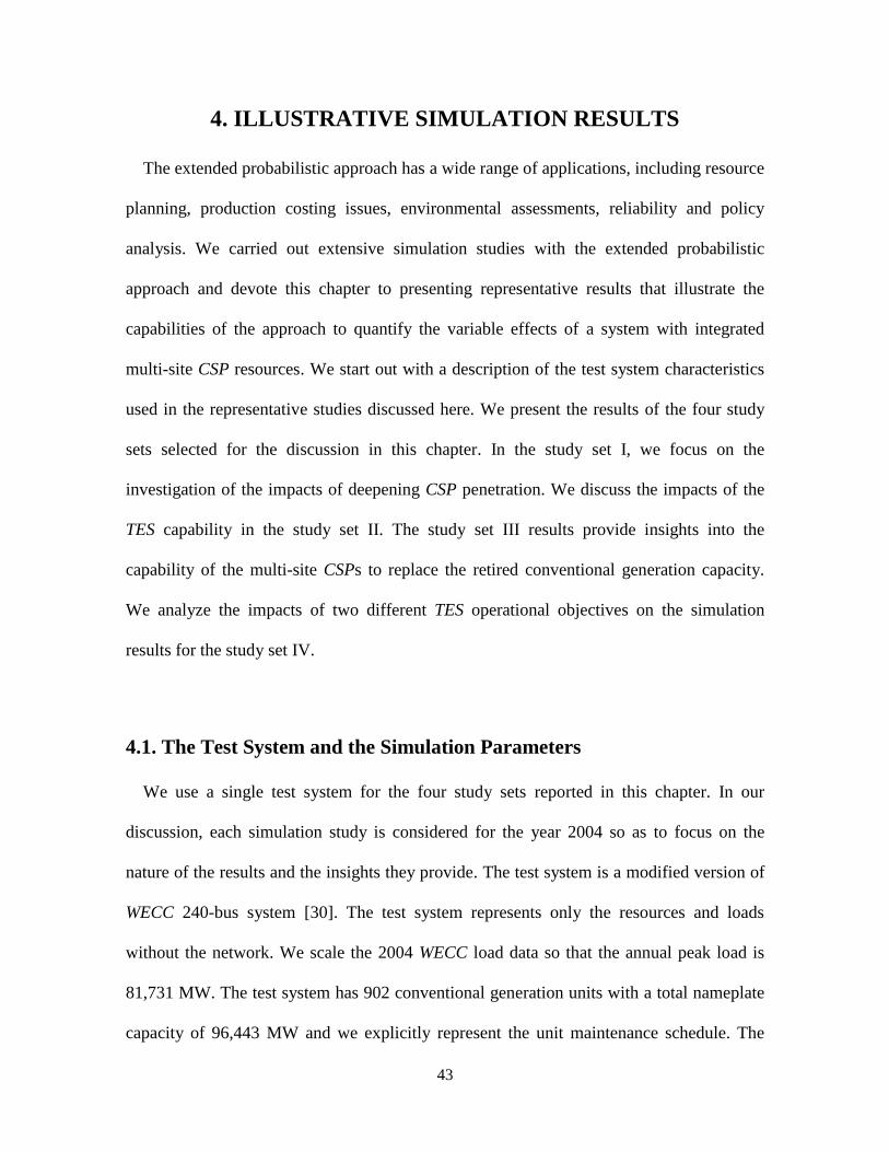
57
Figure 4.9: The annual EUE metric values with/without the 3-hour TES for the set III
sensitivity study
Based on the reliability metrics in study set III, we conclude that the CSP resources
without TES have weak ability to substitute for the retired generation capacity of
conventional units. The incorporation of TES devices can improve considerately this
ability of CSP resources and result in a reduced CSP capacity to replace the retired
conventional unit capacity.
4.5. Study Set IV: Comparison of Two Different TES Operational
Objective Impacts on the Power Systems
The purpose of the study set IV simulations is to compare the impacts of two different
TES operational objectives at the multi-site CSP on the system variable effects. To make
the investigation meaningful in light of the limited controllability of the CSPs without TES,

58
we consider the test system with 1,500-MW total installed CSP capacity with 3-hour TES
at each location with the installations located at only three California sites: Barstow,
Blythe and Lancaster. We compare the results of two case studies: in case 1, the objective
is to maximize the total CSP-produced energy, and in the case 2, the objective is to
maximize the total CSP-produced energy revenues based on forecasted system marginal
prices. We treat case 1 as the base case and compare the values of the metrics of interest, as
well as the additional metric that measures the costs of the CSP energy production under
the two objectives. We normalize all metrics w.r.t. the base case values and display the
results in Fig. 4.10.
Figure 4.10: Comparison of the metric values for the cases of energy maximization (base
case) and revenue maximization for the study set IV
The results in case 1 objective use forecasts of system marginal prices for each hour of
the simulation period. Under the objective in case 2 to maximize the CSP revenues for
energy production, the contribution of the multi-site CSP resources leads to poorer
reliability, higher production costs and higher CO 2 emissions than those under the

59
objective in case 1 to maximize the total CSP energy production. While the CSP owner
receives higher revenues under the case 2 objective for the postulated system marginal
price forecasts, the system is overall worse off. In the objective of case 1, the maximization
assumes that each unit of energy has exactly the same economic value – no time
differentiated system marginal prices as under the case 2 objective. The losses over time in
the energy stored in the TES contribute to the reduction of benefits to the system under the
case 2 optimization.
The study set IV simulations under the two different TES operational objectives provide
insights into the importance of the selected objective. The choice of operational objective
for a CSP has impacts on the overall system benefits gained from CSP resources. Because
different objective functions may produce different results, the CSP owner faces a trade-off
between the improved reliability, environmental metric values of the system and the higher
revenues for CSP-produced energy.
4.6. Summary
In this chapter, we discussed the results of our investigations of the impacts of the CSP
resource spatial and temporal variability on the power system. We have shown the extent
to which the integrated CSP resources and the incorporated TES result in an increase in the
reliability and a reduction in the production costs and in the emissions of the power system.
We have noted that the site choice for CSP installation is an important factor when
investors decide to develop CSP resources. We have also quantified the replacement ability

60
of the multi-site CSP resources with explicit consideration of the variability and
intermittency effects of solar energy.
61
5. CONCLUSION
In this chapter, we summarize the work presented in this thesis and identify directions
for future work.
5.1. Summary
In this thesis, we presented the development and testing of an extended probabilistic
simulation approach to assess, over longer-term periods, the variable effects of systems
with integrated multi-site CSP resources. Throughout the thesis, we described in detail the
successive steps essential to extend the conventional production simulation framework for
systems with integrated multi-site CSP resources. We also present some of the simulation
results we obtained from extensive study so as to demonstrate the capabilities of the
extended tool and the usefulness of our work.
We started with the construction of the deterministic multi-site CSP power output model
– so called SP – which maps the temporally and spatially correlated daily multi-site DNI
data into daily multi-site CSP power outputs. To deal with the uncertainty, variability and
intermittency effects of multi-site DNI data, we utilized the insights we gained to develop
the multi-site DNI model that probabilistically represents the multi-site DNI data. We made
use of the SP and the multi-site DNI model to obtain the probabilistic characterization of
the multi-site CSP power outputs, which we integrated into the extended probabilistic
production simulation tool for systems with the multi-site CSP resources. We selected
representative simulation results to illustrate the influences of multi-site CSP integration on
the system variable effects for a wide variety of parametric studies. Our work provides

62
valuable insights into the role that multi-site CSP resources can play in the effective
harnessing of solar energy and the utilization of TES in the deployment of such resources.
The extension of the probabilistic simulation approach to incorporate the representation
of uncertain, time-varying CSP resources constitutes a significant improvement in the
capability to emulate systems with variable energy resources. The capability to quantify
the impacts of CSP resources on the economics of electricity supply, the emissions and the
system reliability effects make the extended approach very useful for planning, investment
decision, regulatory filing, and policy analysis applications. Our illustrative examples
demonstrate the ability of the approach to answer a broad range of what-if questions on
power systems with integrated multi-site CSPs.
5.2. Future Research
The proposed extension to the conventional production simulation approach is a good
basis to develop a comprehensive simulation framework to evaluate the variable effects of
systems with integrated CSP and wind resources at distinct sites. In addition, we can make
use of the extended simulation tool to investigate the impacts of different TES operational
objectives on the CSP contribution to power systems. We can also explore the stochastic
simulation of systems with integrated CSP resources with the explicit representation of the
day-ahead markets. Indeed, the advantages of the regime-based approach to capture both
the seasonal and diurnal variability of the time-dependent resources can be exploited in
other areas. We will report on such efforts in future publications.

63
APPENDIX A: NOTATION
S number of CSP sites
s subscript to denote the CSP site index with s = 1, 2, …, S
H number of smallest, indecomposable sub-periods from midnight to midnight in
each day in the production simulation framework
h the index of the smallest, indecomposable sub-period with h = 1, 2, …, H
H duration of the sub-period in the production simulation framework, computed
by the ratio of 24 to H
sc CSP nameplate capacity in MW
( )s nonlinear mapping of the DNI into the solar field thermal power output
(s ) nonlinear mapping of the thermal energy flow rate into the CSP power output
in MW
d
s hk rate of charge of thermal energy into the TES in MW t
d
s hv TES charging state status variable {0, 1}
d
s hq rate of discharge of thermal energy from the TES in MW t
d
s h TES discharging state status variable {0, 1}
d
s h thermal energy stored in the TES in MWh t
d
s hz flow rate of thermal energy in MW t to used for electricity generation
d
s h objective function coefficient in the scheduling optimization
min maxs s , lower, upper bound on the TES capability in MWh t

64
min maxs sk k, lower, upper bound on the TES charging capacity in MW t
s TES charging efficiency(0, 1]
min maxs sq q, lower, upper bound on the TES rate of discharge of thermal energy in MW t
s TES discharging efficiency (0, 1]
sψ TES thermal energy loss factor [0, 1]
min maxs sz z, lower, upper bound on the rate of thermal energy delivery for electricity
generation in MW t
I number of days in a seasonal DNI data collection
i superscript to denote the day index of the DNI measurements with i = 1, 2, …, I
i
sM number of DNI measurements collected from each equal-duration sub-period
from sunrise to sunset
m index of the sub-period with m = 1, 2, …, i
sM
M number of equal-duration sub-periods from midnight to midnight with the
identical time resolution as used for the DNI measurements
J number of time-scaled sub-periods in the sunrise-to-sunset period
j index of the time-scaled sub-period with j = 1, 2, …, J
R number of identified DNI clusters
r subscript to denote the index of the identified DNI cluster with 1,2,...,r = R
rR DNI cluster r
rπ probability of the DNI cluster
rR

65
Rr DNI regime r
d superscript to denote the index of the day in the year for a specified season
ˆ i
s mu DNI measurement for the sub-period m
ˆ i
su vector 1 2ˆ ˆ ˆis
T Mi i i iss s s Mu , u , ... , u
i
s jy computed common-time-scaled DNI value used in the clustering analysis
i
sy vector 1 2T
i i i J
s s s Jy , y , ... , y
iY array 1 2
i i J Si
S ... y y y
, ,ˆ ˆ,d b d e
s st t actual sunrise, sunset time
, ,,
d b d e
s sh h sub-period that satisfies ,ˆ{ : }d b
H smax h h t , ,ˆ{ : }d e
H smin h h t
, ,,d b d e
s st t sunrise, sunset time determined by , , , ,
,d b d b d e d e
s s H s s Ht h t h
d
s hU sub-period h DNI r.v.
d
s rhU sub-period h DNI r.v. conditioned on the cluster
rR
d
sU DNI r.v. vector
d
s rU DNI r.v. vector conditioned on the cluster
rR
dU DNI r.v. array
d
rU DNI r.v. array conditioned on the cluster
rR
d
s hu sub-period h computed DNI value obtained from a random sample
dsu vector 1 2
Td d d
s
H
s s Hu , u ... , u
d
s P h sub-period h CSP power output r.v.

66
d
s r
P h sub-period h CSP power output r.v. conditioned on the cluster
rR
d
s p h sub-period h CSP power output
d
sp vector 1 2T
d Hd d
s s sp , p ,, ... , p H
W number of the simulation periods in the study period
w index of the simulation period with w = 1, 2, …, W
T index set of the sub-periods in the simulation period w
E index set of the conventional generation units
wE index set of the committed conventional units in the simulation period w
L load r.v.
hL load r.v. conditioned on sub-period h
kL “remaining” load be served by the blocks of units in the loading list after the
first ( 1k ) blocks are loaded
kL complement of the c.d.f. – the so-called load duration curve (l.d.c.) – of
kL
C controllable load r.v.
J ratio of
i
sM to J

67
APPENDIX B: THE SCALING ALGORITHM
The scaling process is essential to undertake the comparison of the computed DNI data in
a meaningful way. We present the scaling algorithm and state the general expression to
compute i
sy from ˆ i
su . We also provide an illustrative example.
We start out with a statement of the scaling algorithm:
Step B0: Define i
s
J
M
J ; initialize i
s y 0 ; set 0 , j = 1 and 1m .
Step B1: If J
m j , set ˆi i i
s s sj jy y u m m and m and continue; else, go
to step B3.
Step B2: If m =i
sM , go to step B4; else, m = m + 1 and go to step B1.
Step B3: Set ˆi i i
s s s Jj jy y u m j
and J
j and computei
i ss
J
jj
yy
.
Step B4: If j = J , stop; else, set j = j + 1 and go to step B1.
The scaling algorithm may be used to derive the explicit expression for the determination
of i
s jy in the day i at the site s:
1
20 1 2
1
( 1)
Δ
i
s J
i
i is
J s s J
j
y m m j
yy m y m j m
m
mm /
M
MM M M
(B.1)
where
0
1
2
0 1 2 0 1 2
{ : ( 1) , 1 }
{ : ( 1) ( 1) , 1 }
{ : ( 1) ( 1) , 1 }
/ ( ) { : , and }.
i
J J s
i
J s
i
J s
M
M
M
m j m j m
m m j m m
m m j m m
m m m m
M
M
M
M M M M M M

68
We illustrate the scaling process graphically in Fig. B.1. The value of i
sjy
is
determined in terms of the area under the step function for the measured DNI values,
constructed from ˆ i
su , over the duration that corresponds to the common time scale sub-
period j .
(a)
1 2 3 J
common time scale
...
(b)
DN
I (k
W/m
2)
DN
I (k
W/m
2)
Figure B.1. The scaling process uses the measured values of thei
sM sub-periods in the sunrise-to-
sunset period to obtain the common time scale sub-period j computed value i
sjy
, j=1, 2, …, J
1i
sy
2i
sy
3i
sy
i
s Jy

69
APPENDIX C: THE DESCALING ALGORITHM
The descaling process is essential in the determination of the computed DNI data in the
common time scale for a given day d. We present a statement of the descaling algorithm
and derive a formula for the determination of the DNI value d
su h
for each sub-period h
such that d d
b, s e, sh h h in the day d at the site s. We also illustrate the application of the
algorithm with a graphical example.
We start out with a statement of the scaling algorithm:
Step C0: Define 24
HH
,d ,e d ,b
s s
J
t t
J
; initialize d
s u 0 ; set ,
,
d b
d b s
s
H
th
and
,
,
d e
d e s
s
H
th
;
set ,d b
sh , j = 1 and ,d b
sh h .
Step C1: If ,d b
s J Ht j h , set ,d d i d b
s s s s Jh h ju u y t j
and set ,d b
s Jt j ,
continue; else, go to step C3.
Step C2: If j = J, go to step C4; else, set j = j + 1, go to step C1.
Step C3: Set d d i
s s s Hh h ju u y h
and h
h and d
d ss
H
hh
uu
.
Step C4: If h = ,d e
sh , stop; else, set h = h + 1 and go to step C2.
The steps above provide the basis for the explicit expression to determine d
shu for
each h that satisfies , ,d b d e
s sh h h in the day d at the site s. We can show that:
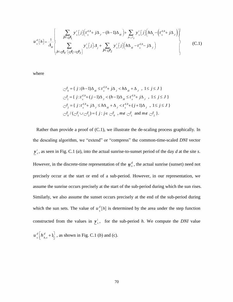
70
2
, ,
1
,
1
20 1 2
1
( 1)i d b i d b
s s J H s s Jj
d
s i i d b
H s j s H s J
j j
hj j
y t j h y h t j
uy y h t j
j
jj
J
/
J
JJ J J
(C.1)
where
,
0
, ,
1
, ,
2
0 1 2 0 1 2
{ : ( 1) , 1 }
{ : ( 1) ( 1) , 1 }
{ : ( 1) , 1 }
/ ( ) { : , and }.
d b
H s J H J
d b d b
s J H s J
d b d b
s J H J s J
j h t j h j J
j t j h t j j J
j t j h t j j J
j j m m
J
J
J
J J J J J J
Rather than provide a proof of (C.1), we illustrate the de-scaling process graphically. In
the descaling algorithm, we “extend” or “compress” the common-time-scaled DNI vector
i
sy , as seen in Fig. C.1 (a), into the actual sunrise-to-sunset period of the day d at the site s.
However, in the discrete-time representation of the dsu , the actual sunrise (sunset) need not
precisely occur at the start or end of a sub-period. However, in our representation, we
assume the sunrise occurs precisely at the start of the sub-period during which the sun rises.
Similarly, we also assume the sunset occurs precisely at the end of the sub-period during
which the sun sets. The value of d
shu is determined by the area under the step function
constructed from the values in i
sy , for the sub-period h. We compute the DNI value
1d d
s b, su h
, as shown in Fig. C.1 (b) and (c).
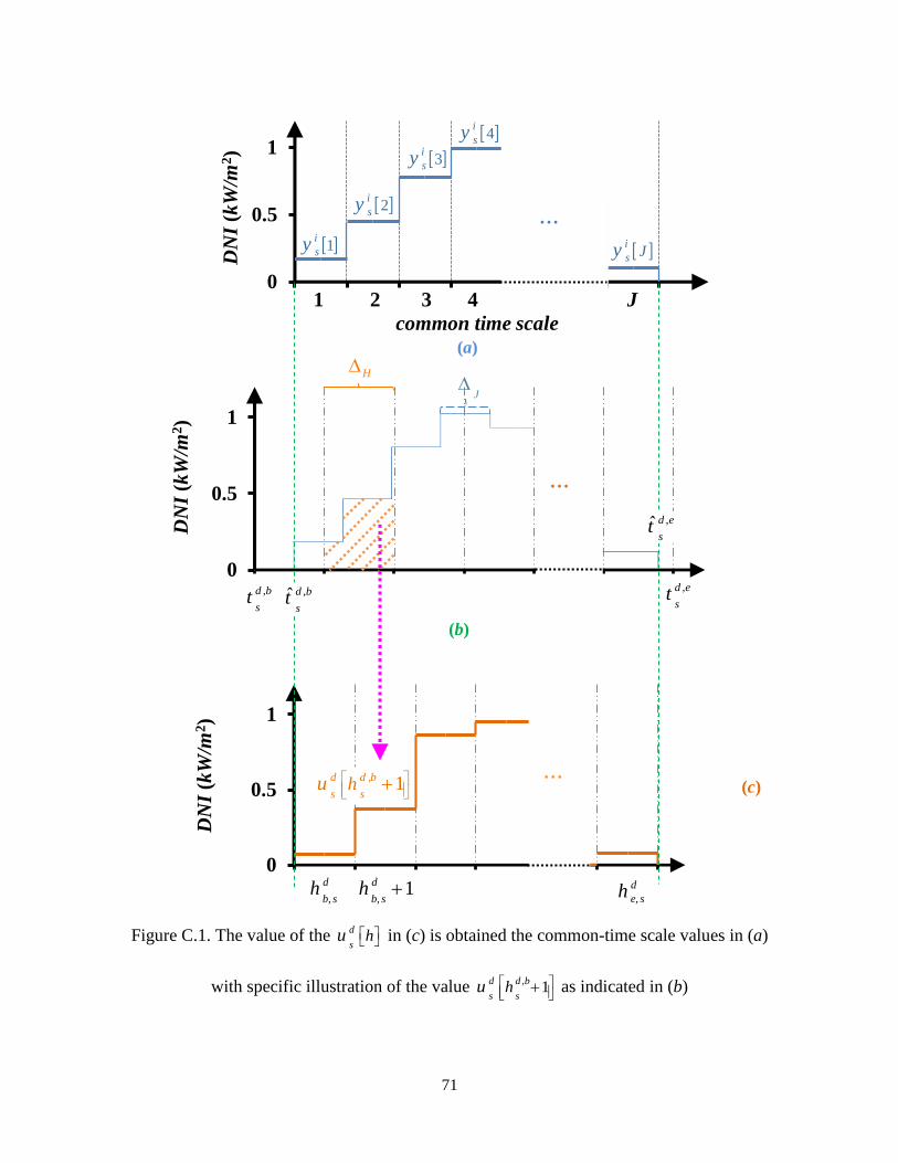
71
Figure C.1. The value of the d
shu in (c) is obtained the common-time scale values in (a)
with specific illustration of the value ,1
d d b
s shu
as indicated in (b)
0
0.5
1
0 2 4 6 8 10 12 141 2 3 4 J
common time scale
...D
NI
(kW
/m2)
0
0.5
1
0 2 4 6 8 10 12
DN
I(k
W/m
2)
...
0
0.5
1
0 2 4 6 8 10 12
...
DN
I(k
W/m
2)
(a)
(b)
(c)
,ˆ d b
st
H
J
1i
sy
2i
sy
3i
sy
4i
sy
i
s Jy
,ˆ d e
st
1d d ,b
s shu
1d
b, sh d
b, sh d
e, sh
,d b
st
,d e
st

72
REFERENCES
[1] DSIRE—Database of State Incentives for Renewables & Efficiency. [Online].
Available: http://www.dsireusa.org/.
[2] P. Brown, “European Union wind and solar electricity policies: overview and
considerations,” 2013. [Online]. Available: https://www.fas.org/sgp/crs/row/
R43176.pdf.
[3] Concentrating Solar Power Projects. [Online]. Available: http:// www.nrel.gov /csp.
[4] U. Wang, “The rise of concentrating solar thermal power,” 2011. [Online]. Available:
http://www.renewableenergyworld.com/rea/news/article/2011/06/the-rise-of
concentrating-solar-thermal-power.
[5] IRENA, “Concentrating solar power,” Renewable Energy Technologies: Cost
Analysis Series, vol.1, no.2, Jun.2012.
[6] CSP Alliance, “The economic and reliability benefits for csp with thermal energy
storage.” [Online]. Available: http://www.csp-alliance.org/updated-cspa-report-
september-2014/.
[7] MIDC – Measurement and Instrumentation Data Center [Online]. Available: http://
www.nrel.gov/midc/.
[8] Sunrise Sunset Calendar [Online]. Available: http:// www. sunrisesunset.com/usa.
[9] CAISO, “Reports and data,” 2014, California Independent System Operator, Folsom,
CA. [Online]. Available: http://www.caiso.com/market/Pages/ReportsBulletins/Daily
RenewablesWatch.aspx.
[10] M. Masters, Renewable and Efficient Electric Power Systems, second edition, John
Wiley & Sons Inc., Hoboken, NJ, 2013.
[11] T. Soubdhan et al., “Classification of daily solar radiation distributions using a
mixture of Dirichlet distributions,” Solar Energy, vol. 83, no. 7, pp. 1056-1063, July
2009.
[12] E. Lorenz et al., “Irradiance forecasting for the power prediction of grid-connected
photovoltaic systems,” IEEE Journal of Selected Topics in Applied Earth
Observations and Remote Sensing, vol. 2, no. 1, pp. 2-10,Jan. 2009.
[13] S. Madaeni et al., “Estimating the capacity value of concentrating solar power plants:
A case study of the southwestern United States,” IEEE Trans. Power Syst., vol. 27,
no. 2, pp.1116–1124, May 2012.

73
[14] R. Sioshansi and P. Denholm, “The value of concentrating solar power and thermal
energy storage,” IEEE Trans. Sustain. Energy, vol. 1, no. 3, pp. 173–183, Oct. 2010.
[15] R. Dominguez et al., “Optimal offering strategy for a concentrating solar power
plant,” Applied Energy, vol. 98, pp.316-325, 2012
[16] Y. Zhang and S. Smith, “Long-term modeling of solar energy: analysis of
concentrating solar power (CSP) and PV technologies,” 2011. [Online]. Available:
http://www.pnl.gov/main/ publications/external/technical_reports/pnnl-16727.pdf
[17] D. Halamay and K. Ted, “Monte Carlo analysis of the impacts of high renewable
power penetration,” in 2011 IEEE Energy Conversion Congress and Exposition
(ECCE), Sep. 2011, pp. 3059-3066.
[18] J. Price and J. Goodin, “Reduced network modeling of WECC as amarket design
prototype,” in Proceedings of the IEEE PES General Meeting, Detroit, July 24-28
2011, pp. 1-6.
[19] M. Milligan, “Methods to model and calculate capacity contributions of variable
generation for resource adequacy planning (IVGTF1-2): Additional discussion,”
National Renewable Energy Laboratory, Atlanta, GA, Tech. Rep., Jan. 2011.
[20] A. Wood, B. Wollenberg and G. Sheblé, Power Generation, Operation and Control,
John Wiley & Sons Inc., Hoboken, NJ, 2013.
[21] S. Karaki et al., “Probabilistic performance assessment of autonomous solar-wind
energy conversion systems,” IEEE Trans. Energy Convers., vol. 14, no.3, pp. 766–
772, Sept. 1999.
[22] NREL, “Solar Advisor Model,” 2012, National Renewable Energy Laboratory,
Golden, CO. [Online]. Available: https://sam.nrel.gov/.
[23] A. Rovira et al., “Energy management in solar thermal power plants with double
thermal storage system and subdivided solar field,” Applied Energy, vol.88, no.11, pp.
4055-4066, Nov. 2011.
[24] J. Usaola, “Operation of concentrating solar power plants with storage in spot
electricity markets,” IET. Renewable Power Generation, vol. 6, no.1, pp. 59-66, Jan.
2012.
[25] K. Powell and T. Edgar, “Modeling and control of a solar thermal power plant with
thermal energy storage,” Chemical Engineering Science, vol. 71, pp. 138-145, Mar.
2012.

74
[26] R. Bhana, “A production simulation tool for systems with integrated photovoltaic
energy resources.” Dept. Elect. & Comput. Eng. Univ. Illinois, Urbana-Champaign,
2011.
[27] R. Xu and D. Wunsch, “Partitional clustering”, in Clustering, John Wiley & Sons
Inc., Hoboken, NJ, pp. 67-72, 2009.
[28] N. Maisonneuve and G. Gross, “A production simulation tool for systems with
integrated wind energy resources,” IEEE Trans. Power Syst., vol. 26, no. 4, pp. 2285-
2292, Nov. 2011.
[29] G. Gross, “Electricity Resource Planning,” class notes for ECE 588, Dept. Elect. &
Comput. Eng. Univ. Illinois, Urbana-Champaign, Fall 2012.
[30] J. Price and J. Goodin, “Reduced network modeling of WECC as a market design
prototype,” in Proceedings of the IEEE PES General Meeting, Detroit, July 24-28
2011, pp. 1-6.
[31] NOAA, “Climate data for stations,” National Oceanic and Atmospheric
Administration, Silver Spring, MD. [Online]. Available:
http://www7.ncdc.noaa.gov/CDO/dataproduct.
[32] Y. Degeilh and G. Gross, “Stochastic simulation of power systems with integrated
intermittent renewable resources,” submitted to IEEE Trans. on Power Systems.