a precise measurement of the left-right asymmetry …
TRANSCRIPT
SLAC-452 UC-414
(W
A PRECISE MEASUREMENT OF THE LEFT-RIGHT ASYMMETRY OF 2 BOSON PRODUCTION
AT THE SLAC LINEAR COLLIDER
Ross C. King Stanford Linear Accelerator Center
Stanford University, Stanford, CA 94309
September 1994
Prepared for the Department of Energy under contract number DE-AC03-76SF00515
Printed in the United States of America. Available from the National Technical Information Service, U.S. Department of Commerce, 5285 Port Royal Road, Springfield, Virginia 22161.
*Ph.D. thesis.

Abstract
We present a precise measurement of the left-right cross section asymmetry of Z boson pro-
duction (A& observed in 1993 data at the SLAC linear collider. The A, experiment
provides a direct measure of the effective weak mixing angle through the initial state cou-
plings of the electron to the Z. During the 1993 run of the SLC, the SLD detector recorded
49,392 Z events produced by the collision of longitudinally polarized electrons on unpolar-
ized positrons at a center-of-mass energy of 9 1.26 GeV. A Compton polarimeter measured
the luminosity-weighted electron polarization to be (63.4 + 1.3)%. Am was measured to be
0.1617 X!I O.O071(stat.) + O.O033(syst.), which determines the effective weak mixing angle
to be sin 2 0, eff = 0.2292 + O.O009(stat.) + O.O004(syst.). This measurement of ALR is incom-
patible at the level of two standard deviations with the value predicted by a fit of several
other electroweak measurements to the Standard Model.
ii

Acknowledgments
First thanks go to my adviser, Morris Swartz, for knowing everything about particle physics
and statistics as well, and for always having the time and patience to teach me.
Thanks also to:
Peter Rowson, Mike Woods, Mike Fero, Dave Calloway, and Bruce Schumm, for provid-
ing further instruction and camaraderie, as well as for creating and maintaining the spirit of
the Compton Cowboy.
My fellow graduate students, Amit Lath and Tom Junk, for sharing their knowledge and
skills during our tenure together. Special thanks to Kevin Pitts, John Yamartino, Ram Ben-
David, and Rob Elia, for paving the way.
David Williams, for tips on PAW, and Suzanne Williams, for help with FRAMEMAKER,
publications plots, and for the food.
And finally, thanks to my wife, Karin, for providing me with the incentive to reach my pri-
mary goal: being able to bench-press my own weight. Thanks also for the incentive
necessary to finish this document. : )
iii

Table of Contents
Abstract ii
Acknowledgments iii
List of Tables ix
List of Figures X
Chapter 1: Physics Background and Motivation 1
1.1 TheStandardModel.. ............................................. .2
1.1.1 TheGaugeBosons ........................................... .2
1.1.2TheFermions ................................................ .
1.1.3 Spontaneous Symmetry Breaking ................................ .4
1.2 The 2 Production Cross Section ..................................... .7
1.2.1 Defining Polarization .......................................... 8
1.2.2ThePhotonExchange.. ........................................ .
1.2.3TheZExchange .............................................. .
1.2.4 Z-y Interference .............................................. 10
1.3 Standard Model Tests ............................................. 11
1.3.1 Electroweak Asymmetries ..................................... 12
1.3.2 Width of the Z Resonance ...................................... 14
1.4 Radiative Corrections .............................................. 16
iv

1.4.1 Initial State Radiation ......................................... 16
1.4.2 Oblique Corrections .......................................... 17
1.4.3 Vertex Corrections .......................................... .20
1.4.4 Box Corrections ............................................. 21
1.4.5 QCD Corrections ............................................ 21
1.5 Properties of Am ................................................ .21
1.51 The Measured Left-Right Asymmetry ........................... .22
1.52 Advantages of Am .......................................... .23
1.6 The Weak Mixing Angle .......................................... .24
1.6.1 s: ...................................................... ..2 5
1.6.2 ~5 and sz .................................................. 25
-1.6.3 sin20~....................................................2 6 1.6.4 Converting to the Weinberg Angle .............................. .27
1.7 Thesis Outline .................................................. .28
Chapter 2: Experimental Apparatus
2.1ThePolarizedSLC................................................2 9 2.1.1 Polarized Electron Source ..................................... .31
2.1.2 Flat Beam Operation ......................................... .39
2.1.3 Spin Dynamics ............................................. .40
2.1.4SpinTransport...............................................4 0
2.2 Mplller Polarimetry ............................................... .46
2.2.1 MollerTargets .............................................. .48
2.2.2 The Extraction Line Moller Polarimeter .......................... .48
2.2.3 The Linac Moller Polarimeter .................................. .50
2.3 The Compton Polarimeter ......................................... .51
2.3.1 The Compton Polarized Target ................................. .53
2.3.2 The Cherenkov Detector ...................................... .58
2.3.3 The Proportional Tube Detector ................................ .61
V

2.3.4 Data Acquisition ............................................ .63
2.4 The Energy Spectrometer ......................................... -66
2.5 The SLD Detector ............................................... .67
2.5.1 SLD Subsystems ............................................. 68
2.5.2 The Liquid Argon Calorimeter ................................. .70
Chapter 3: Compton Polarimetry 73
3.1 Compton Scattering Kinematics .................................... .73
3.1.1 Laboratory Frame Scattering Kinematics ......................... .75
3.1.2 Radiative Corrections ........................................ .76
3.2 Extracting the Beam Polarization from Compton Scattering .............. .77
3.2.1 The Analyzing Bend Magnet .................................. .78
3.2.2 The Experimental Asymmetry ................................. .79
3.3 Measuring the Experimental Asymmetry ............................. .8 1
3.3.1 Compton Asymmetries ....................................... .81
3.3.2 Detector Linearity ........................................... .82
3.3.3 Electronic and Laser Noise Pickup .............................. .85
3.3.4 Saturated Pulses ............................................. 87
3.4 Determination of the Analyzing Powers .............................. .87
3.4.1 Endpoint Calibration ......................................... .88
3.4.2 Zero Asymmetry Point ....................................... .89
3.4.3 The Beamstrahlung Shield .................................... .91
3.4.4 Detector Response Function ................................... .92
3.4.5 Interchannel Consistency ..................................... .94
3.5 Target Polarization ............................................... .96
3.5.1 optics ........................................... ......... .96
3.5.2 Pre-AUTOPOCKSCAN Analysis .............................. .98
3.5.3 AUTOPOCKSCAN Analysis .................................. 101
3.6 Absolute Sign Determination ....................................... 103
vi

3.6.1 Sign of the Compton Scattering Asymmetry ...................... 104
3.6.2 Helicity of the Target Photons ................................. 105
3.7 Polarimeter Data Selection ........................................ 107
3.7.1 Run-specific Cuts ........................................... 108
3.7.2 Channel-specific Cuts ........................................ 109
3.7.3 TheFinalComptonPolarization ................................ 111
3.8 Polarimeter Systematic Errors ...................................... 111
3.9 The Luminosity-weighted Polarization ............................... 112
Chapter 4: 2 Event Selection and Background Estimation
4.1 The LAC Energy Scale ........................................... 114
4.2 Event Triggers .................................................. 115
4.2.1Muons.. ................................................ ..116
4.2.2 LAC ENERGY Trigger ...................................... 116
4.3 Selection Criteria ................................................ 117
4.3.1 Pass One Selection .......................................... 117
4.3.2EventReconstruction ...................................... ..119
4.3.3 Pass Two Selection .......................................... 119
4.3.4 Polarimeter Cuts ............................................ 122
4.3.5 Result .................................................... 124
4.3.6 Tracking-based Event Selection ................................ 124
4.4 Background Estimation ........................................... 125
4.4.1Bhabhas...................................................12 5
4.4.2 Cosmic Rays ............................................... 135
4.4.32~Events..................................................13 6
4.4.4yyEvents.. .............................................. ..13 7
4.4.5 Beam Background Events ..................................... 137
4.4.6 Background Summary ....................................... 140
4.5 The Background Asymmetry ....................................... 140
vii

Chapter 5: Analysis and Results 142
5.1 The Chromaticity Effect .......................................... 142
5.1.1 The Chromaticity Model ...................................... 143
5.2 Additional Corrections to Au ...................................... 149
52.1 Luminosity Asymmetry ...................................... 150
5.2.2 Energy Asymmetry .......................................... 150
5.2.3 Efficiency Asymmetry. ....................................... 15 1
5.2.4PositronPolarization.........................................15 1 5.2.5 Summary of Small Corrections ................................ .152
5.3 Systematic Cross-checks .......................................... 153
5.3.1 Fixed Polarizer Test ......................................... 153
5.3.2 Current Asymmetry Test. ..................................... 153
5.3.3 IP-Compton Spin Precession .................................. 155
5.3.4 Bit Integrity ................................................ 156
5.3.5 Helicity Synchronization ..................................... 157
5.3.6 Cut Bias ................................................... 158
5.3.7 Total Systematic Uncertainty .................................. 161
5.4 Results and Comparisons .......................................... 162
5.4.1 Extracting Am .............................................. 162
5.4.2 Extracting the Weinberg angle from A,TJ ......................... 162
5.4.3 Comparison with LEP data .................................... 163
5.4.4 Comparison with the Standard Model ........................... 164
5.5 Future Experimental Precision ...................................... 166
References 168
viii

List of Tables
l-l The couplings of fermions to the Z in the Standard Model ................. .7
l-2 Present experimental parameterization of the Standard Model. ............. 11
l-3 Properties of various electroweak asymmetries. ........................ .24
2-l Results of Linac Mgller Polarimeter measurements. ..................... .51
3-l 1993 Endpoint Scan Results ........................................ 89
3-2 Nominal Positions and Analyzing Powers by Period .................... .91
3-3 Ideal and Corrected Analyzing Powers ................................ 93
3-4 Thick and Thin Pre-radiator Comparison ............................. .94
3-5 Results of best fits to the Cherenkov spectrum. ......................... .94
3-6 P, measurements during the pre-AUTOPOCKSCAN era. ................ 100
3-7 Inferred Electron Helicity during 1993 run ............................ 106
3-8 Total Systematic Error for Individual Channels and Combined Channels .... 112
4-l Results of Method 1 Bhabha background estimate: Barrel Region .......... 131
4-2 Results of Method 1 Bhabha background estimate: Endcap Region ......... 131
4-3 Summary of 1993 background estimate. .............................. 140
5-l Parameters of beam transport simulation. ............................. 148
5-2 Summary of corrections to Au. ..................................... 152 5-3 Total systematic uncertainty on the A, measurement. ................... 161
5-4 Converting the observed value of ALR into ALR ........................ 163
5-5 ZFI’M’ER predictions for top mass and Au at the Z peak ................ 165
ix

List of Figures
l-l Fermions in the Standard Model. ...................................... 3
l-2 Definition of the weak mixing angle. ................................. .6
l-3 Standard Model tree-level process e -e+ + ff. ......................... .8
l-4 Initial state radiation. .............................................. 16
l-5 Radiative corrections to the Z peak cross section. ........................ 17
l-6 Families of oblique corrections. ...................................... 18
l-7 Lowest order electroweak vertex diagrams. ........................... .20
l-8 Lowest order electroweak box diagrams. .............................. 21
2-l ThePolarizedSLC................................................3 0
2-2 The SLC polarized electron source .................................. .32
2-3 Energy level diagram for a Gallium Arsenide photocathode ................ 32
2-4 Energy level diagram for a strained Gallium Arsenide photocathode ......... 34
2-5 Measurements of various photocathode materials ....................... .35
2-6 The SLC Polarized Electron Gun ................................... .38
2-7 The time history of SLC luminosity. ................................. .39
2-8 Spin rotation in the North Damping Ring ............................. .41
2-9 General spin rotation system ....................................... .42
2-10 Vertical orbit and spin components over the first 23 achromat sections ...... .44
2-11 The dependence of polarization on energy ............................ .46
2-12 The extraction line MoIIer polarimeter ................................ 49
X

2-13 2-14
2-15
2-16
2-17
2-18
2-19
2-20
2-21 2-22
2-23
2-24 2-25
2-26
3-l 3-2
3-3
3-4
3-5
3-6
3-7
3-8
3-9
3-10
3-11
3-12
3-13
3-14
The linac Moller polarimeter. ....................................... 50
The Compton polarimeter .......................................... 53
The CLS laser bench. ............................................. .54
The Compton laser transport system. .................................. 56
The CLS analysis box optics ....................................... .58
Overhead view of the Compton Cherenkov and proportional tube detectors. .. .59
The Compton proportional tube detector. .............................. 61
The PTD electronics ............................................. .62
The PTD linearity from 1993 data. ................................... 63
Schematic representation of the Compton polarimeter data acquisition ...... .64
The electron extraction line energy spectrometer. ........................ 66
Cutaway view of the SLD detector. .................................. .68
Quadrant view of the SLD detector. ................................. .71
LACbarrelEMandHADmodules .................................. .72
Tree-level Compton scattering. ..................................... .74
The Compton cross section and asymmetries. .......................... .77
The analyzing bend magnet of the Compton polarimeter. ................. .78
Luminosity-weighted Compton Asymmetries .......................... .83
Cherenkov Channel 6 Linearity Calibration ............................ 84
Cherenkov Channel 7 Linearity Calibration ............................ 85
A time history of the laser noise pick-up for Cherenkov channel 6. .......... 86
Monte Carlo results showing the effect of saturated pulses. ............... .88
Compton kinematic edge scan. ..................................... .89
Time history of the location of the Compton zero-asymmetry point. ........ .90
Cherenkov detector response function for channel 7 ...................... .93
Comparison of the measured Compton asymmetry and the theoretical asymmetry, including the EGS detector response function. ............... .95
Introduction of an arbitrary phase shift. ................................ 97
pr” in the Pre-AUTOPOCKSCAN era. .............................. 100
xi
3-15 Time history of Pr during the AUTOPOCKSCAN era. .................. 103
3-16 The 1993 Compton measured polarization. ............................ 113
4-l Pass One events in EHI-EL0 space .................................. 118
4-2 Pass One events in Energy versus Imbalance space ..................... 121
4-3 Tree-level Bhabha scattering ....................................... 122
4-4 A summary of the Pass Two event selection. ......................... .123
4-5 Normalized cluster multiplicity distributions for Bhabha and hadronic events. 127
4-6 Bhabha selection Method 1 ....................................... .129
4-7 The distributions of EEHIl+EEHI2 and EHTOT ....................... 130
4-8 Bhabha selection Method 2. ........................................ 134
4-9 (A) The 2y process. (B) The ‘yy process. .............................. 136
4-10 The Pass One data in I versus iVclus variable space. ...................... 138
4-11 Imbalancedistributions ......................................... ..13 9
4-12 The angular distribution of the identified Bhabha sample. ................ 141
5-l (a) N,-(E), (b) o,,(E), and (c) P,(E) in the chromaticity model. ............. 145
5-2 The position of the SL-3 collimator vs. the measured Compton polarization. . 147
5-3 Predictions of the chromaticity model. ............................... 149
5-4 The fixed-polarizer test. ........................................... 154
5-5 The induced current asymmetry test. ................................. 155
5-6 The PLS/CLS pseudo-random number generator. ....................... 156
5-7 The measured asymmetry versus Pass Two cut variables ................. 159
5-8 The measured asymmetry versus other event variables. .................. 160
5-9 A comparison of LEP and SLD sin20f measurements. ................. 164
5-10 The projection of electroweak observables in S-T space. ................. 165
5-11 Standard Model fit to electroweak observables. ........................ 167
5-12 The projected error on the effective weak mixing angle. ................. 167
xii

Chapter 1
Physics Background and Motivation
The SLAC’ Linear Collider (SLC) is a machine designed to accelerate and collide electrons and positrons at high energy (50 GeV per beam). Recent upgrades to the SLC electron
source allow for the production of spin-polarized electron bunches. The use of polarized
electrons at SLC opens a unique window to the world of electroweak interactions. Elec-
troweak asymmetries in particular offer systematically clean experiments with a high
sensitivity to new physics. The left-right asymmetry of Z boson production, known as Am,
provides a particularly good probe of electroweak radiative corrections. The measurement
of Am is the principle goal of the current SLC/SLD program [ 11, and a detailed description
of this measurement using data recorded during 1993 is the topic of this document.
In this chapter, we will outline the theory of electroweak interactions and its predictions
for the 2 production cross section and various related asymmetries. We will describe vari-
ous tests of the theory and the advantages of A m in particular. Finally, we will discuss the
effect of radiative corrections, and a parameterization of these corrections that includes the
effects of new physics.
1. Stanford Linear Accelerator Center
1
I .I The Standard Model 2
1.1 The Standard Model
During the 1960’s, Glashow [2], Salam [3], and Weinberg [4] constructed a new model of
particle interactions that unified the weak and electromagnetic forces. This model is now
known as the Standard Model of Electroweak Interactions, or simply the Standard Model,
as it will be referred to throughout this document. This theory is concerned with the unifi-
cation of the electromagnetic and weak nuclear forces (to be distinguished from Quantum Chromodynamics, or QCD, the theory of the strong nuclear force). The Standard Model has
so far proven to be very successful, predicting, among other things, the existence of a mas-
sive neutral intermediate vector boson, the Z boson.
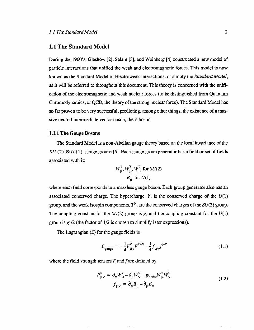
1.1.1 The Gauge Bosons
The Standard Model is a non-Abelian gauge theory based on the local invariance of the
SU (2) @ U ( 1) gauge groups [Sj. Each gauge group generator has a field or set of fields
associated with it: W$ Wi, Wi for SU(2)
B, for U(1)
where each field corresponds to a massless gauge boson. Each group generator also has an
associated conserved charge. The hypercharge, Y, is the conserved charge of the U(1)
group, and the weak isospin components, p, are the conserved charges of the SU(2) group.
The coupling constant for the SU(2) group is g, and the coupling constant for the U(1)
group is g’/2 (the factor of l/2 is chosen to simplify later expressions).
The Lagrangian (0 for the gauge fields is
where the field strength tensors F andfare defined by
F;V = a,w; - a,w: + g&&,w;w~
f pv = v, - $4
(1.1)
(1.2)
I .l The Standard Model 3
In these expressions, 3, = a/ax’, and &abc is the completely anti-symmetric Levi-Chivita
tensor.
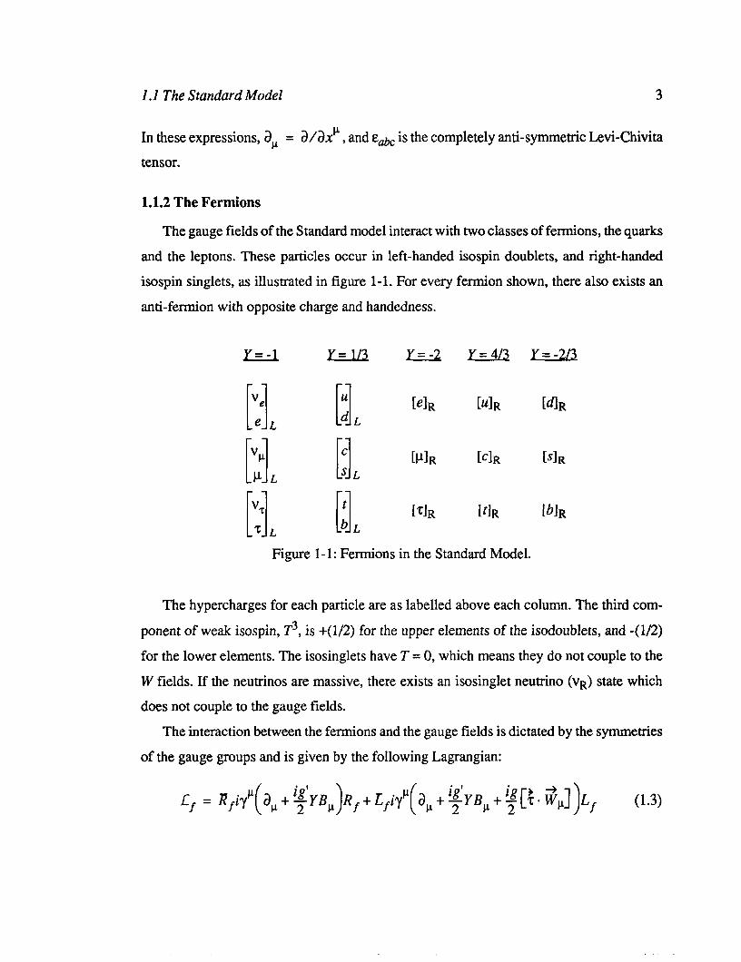
1.1.2 The Fermions
The gauge fields of the Standard model interact with two classes of fermions, the quarks
and the leptons. These particles occur in left-handed isospin doublets, and right-handed
isospin singlets, as illustrated in figure l-l. For every fermion shown, there also exists an
anti-fermion with opposite charge and handedness.
y=-1 Y= l/3 y=-2 y=4/3 y=-2/3
iL iL Ie]R L”]R [6JR
1 L [:I, [p]R Fc]R IsIR
[::I, [;jL i2]R rt]R Ib]R
Figure l-l: Fermions in the Standard Model.
The hypercharges for each particle are as labelled above each column. The third com-
ponent of weak isospin, T3, is +(1/2) for the upper elements of the isodoublets, and -(l/2)
for the lower elements. The isosinglets have T = 0, which means they do not couple to the
W fields. If the neutrinos are massive, there exists an isosinglet neutrino (vR) state which
does not couple to the gauge fields.
The interaction between the fermions and the gauge fields is dictated by the symmetries
of the gauge groups and is given by the following Lagrangian:
Lf = Kfiy’(a,+~YB,)Rf+Lfiy’(a,+~YB,+~[:.~~])Lf (1.3)

I .I The Standard Model 4
where R f = f(1 +ys)f and Lf = f ( 1 - yS) f are general fermion isosinglets and iso-
doublets, f are the Dirac matrices, and % is the generator of SU(2) rotations, normally rep-
resented by the Pauli matrices.
1.1.3 Spontaneous Symmetry Breaking
One difficulty of the theory at this point in its development is that the gauge bosons are
all massless. This is all well and good for electromagnetism, but the weak nuclear force is
observed to have a finite range which implies that a massive boson is exchanged. Another problem is that global SU(2) invariance prevents us from writing down any mass terms for
our fermions, which are of course observed to have mass. The ingenious solution to this problem was suggested by Higgs (for whom the Higgs
boson is named) and others [6]. Weinberg and Salam applied these ideas by introducing a
complex doublet of scalar fields
(1.4)
which transforms as and SU(2) isodoublet with hypercharge Yq = 1. We then add some new
terms to the overall Lagrangian, first
where tc and p are dimensional parameters and the covariant derivative D, is defined by
D, = a,+$YB,+$[:.&]. (1.6)
In addition, we wish to couple the scalar field (the Higgs field) to the fermions, which is
accomplished through a Yukawa-type interaction Lagrangian:
L cp, f = A, [Rf (q+Lfl + Lf ((PRf) I (1.7)
where $ is an arbitrary dimensionless constant. This interaction is invariant under
SU (2) QD U ( 1) transformations and is a Lorentz scalar.

1 .l The Standard Model 5
Now we assume I&O and expand the Higgs field about the minimum of the scalar potential, 2) = 4/-lc2/lpI :
cp = GP,) + O = [ 1 rl/Jz where (‘po) is the vacuum expectation value of the scalar field, which breaks both the isos-
pin and hypercharge symmetries, and TJ is the perturbation of the vacuum. The only
remaining symmetry in the theory is the strange combination of operators
(T3+;Y)@J = Q<q,> = 0 (1.9)
where Q is now identifiable as the electric charge operator. This is the essence of the spon-
taneous-symmetry breaking process: the original gauge symmetries are broken, leaving
only the physically observed conserved quantity, the electric charge.
Expanding various terms in the Lagrangian about the vacuum expectation value of the
Higgs field has very interesting results:
L ‘(a”q)@,q) -~~q~+$[g~1W;-iW;~~+(g.BpgW:)3 scalar = 2 (1.10)
plus interaction terms. The IJ field has become the physical manifestation of the Higgs
boson with mass mi = -2~~. We further identify the charged gauge fields
with a mass of RZ W’
= gu/2, and a neutral gauge field
zP = cosBwWl - sin0,B,
(1.11)
(1.12)
where we have introduced the weak mixing angle, Ow, which is related to the original gauge
coupling constants as shown in figure 1-2.

I .l The Standard Model 6
Figure l-2: Definition of the weak mixing angle.
This neutral field has a mass mZ = mw/cosBw . The orthogonal combination of the orig-
inal gauge fields yields an additional neutral field
A, = sinBwWi + COS~~B,, (1.13)
which is massless. A, may now be identified as the vector potential of the photon field.
The Yukawa potential of equation (1.7) now has the form
(1.14)
which introduces a mass term for the fermions, as well an interaction term for fermions with
the physical Higgs, q. Unfortunately, the constants $ are arbitrary and offer no real insight
into the question of fermion mass.
The interaction Lagrangian now has two distinct parts: the charged-current part and the
neutral current part. The charged-current interaction for leptons has the following form:
.c charged = ~2[vfYpu -Y~)fW;+.TY”(l -Ys)vfwJ (1.15)

1.2 The Z Production Cross Section 7
and the neutral-current interaction for leptons, expressed in terms of electroweak operators,
is given by
L = gsinewJj~fA,-gsinew~~~ 2sin2ew
neutral sin28, Qf fZP I (1.16)
This interaction can be compactly written as
L neutral = efy’f A, - e.M bf - afYsl fz, (1.17)
where we have identified the electric charge, e = g sin 8,) and the vector (vf) and axial
vector (af) coupling constants are defined as follows
Vf = T; - 2sin20,Qf /sin28, .
af = T;/sin2tIw
The values of these constants for all fermions in the theory are listed in table l-l.
Fermion
v,, vp v,
e-, pm, 2-
u, c, t
d, s, b
af. sin28w
1 z
-- 1 2
1 z
1 -- 2
vfe sin2eW
1 z
-- 1 + 2sin2ew 2
23 tsin2e w 1 -
l -23 + hI12e w
Table l-l: The vector and axial-vector couplings of fermions to the Z in the Standard Model
1.2 The 2 Production Cross Section
(1.18)
At this point we wish to demonstrate what physics can be explored with a polarized elec-
tron/positron collider. The Standard Model provides the tools necessary to calculate the
cross section for the process e-e+ + ff, which is diagrammed in figure l-3. The special
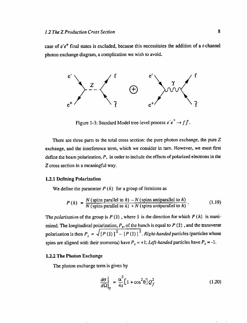
1.2 The Z Production Cross Section 8
case of e-e+ final states is excluded, because this necessitates photon exchange diagram, a complication we wish to avoid.
the addition of a t-channel
Figure l-3: Standard Model tree-level process e-e+ + ff .
There are three parts to the total cross section: the pure photon exchange, the pure Z
exchange, and the interference term, which we consider in turn. However, we must first
define the beam polarization, P, in order to include the effects of polarized electrons in the
Z cross section in a meaningful way.
1.2.1 Defining Polarization
We define the parameter P (2) for a group of fermions as
P(A) = N (spins parallel to ii) - N (spins antiparallel to A) N (spins parallel to 2) + N (spins antiparallel to 2) *
(1.19)
The polarization of the group is P (i) , where 2 is the direction for which P (;i) is maxi-
mized. The longitudinal polarization, P,, of the bunch is equal to P (2) , and the transverse
polarization is then P, = [P (S) ] 2 - [P (2) ] 2. Right-handed particles (particles whose
spins are aligned with their momenta) have P, = +l; Left-handed particles have Pz = - 1.
1.2.2 The Photon Exchange
The photon exchange term is given by
do dny
= $1 +cos20]Q; (1.20)

1.2 The Z Production Cross Section 9
where a is the fine-structure constant, equal to the electric charge-squared divided by 47c,
s is equal to the center-of-mass energy-squared, and 8 is the polar angle and Qftbe electric
charge of the emergent fermion.
AttheZpole(s = rni ) the photon exchange cross section is approximately 800 times
smaller than the Z-exchange. The photon exchange is a parity-conserving process that
dilutes any electroweak asymmetry and must be accounted for in a precision measurement.
1.2.3 The Z Exchange
Given our definition of polarization, the complete polarization-dependent Z pole cross
section in the limit of light final state fermions (p + 1) is
(1.21)
+(p:-P;)[2( 1 +c2)v~a~(v~+a~)+4c(v:+af)vfaf]
where a is the electromagnetic fine structure constant, s is the square of the center of mass
collision energy, r, is the resonant width of the Z, and c is the cosine of the polar angle of
the outgoing fennion. The superscripts “-” and “+” refer to the electron and positron beams,
respectively. The subscripts “3 and 7” refer to longitudinal and transverse polarization
components, respectively. The angle <D is defined by 0 = 2$- @- - 0’ , where + is the azi-
muthal angle of the outgoing fermion, and $* are the azimuthal angles of the electron and

I .2 The Z Production Cross Section 10
positron transverse polarizations. Equation (1.21) simplifies somewhat in the case of lon- gitudinal electron polarization only:
do dn :Iz = cmzx
f ((1 +c2)(v:+at)(v;+a:)+8cvp,vfaf
(1.22)
-p,[2( 1 +c2)vea,(v;+a$+4c(vf+af)vfaf]l
where the longitudinal polarization of electrons is now denoted as P,, a definition that will
be used throughout this document. We can integrate equation (1.22) over the symmetric
detector acceptance limit x (a symmetric co& limit) to find
(1.23)
We will show that the asymmetry term A, is equivalent to A, in section 1.3.1. The gm-
metric factor F(x) is given by
F(x) = (1.24)
1.2.4 Z-y Interference
The Z-y interference term is given by
(1.25)
{( ) 1 + c* v,vf + 2ca,af-P, [ ( 1 1 + c* vfa, + 2cveaf] }

I .3 Standard Model Tests 11
which vanishes rigorously at the Z pole. However, due to the effects of initial state radia-
tion, no real experiment takes place at exactly the Z pole energy. Therefore the interference
diagram, which does have parity-violating terms, must be taken into account for precision
electroweak measurements.
1.3 Standard Model Tests
It is the goal of electroweak physics to test the Standard Model to the limits of experi-
mental precision. However, no single measurement is sufficient for this task. I
Parameter Standard Model Dependence Value a gg’/4r( g2 + s12J 1 / 137.0359895(61) [7]
GF 1/[J%12] 1.16637(2) x 10m5 GeV2 [7]
“2Z Jii
91.190(4) GeV [8]
Table l-2: Present experimental parameterization of the Standard Model.
At tree level, low-energy (& 5 100 GeV ) electroweak phenomena depend on three
parameters of the Standard Model: the gauge coupling constants g and g’, and the vacuum
expectation value of the Higgs field, u/A. These parameters have been accurately spec-
ified by the measurements listed in table l-2. However, beyond tree-level, higher order (loop-level) corrections involve summations
over all heavy particles (heavy meaning m2/s for a given particle is not negligible). There-
fore, electroweak observables are sensitive to the Standard Model Higgs boson mass (mH)
and the top quark mass (ml), as well as to heavy physics beyond the Standard Model. At
present, the Higgs mass is unknown, and the top mass is only weakly specified [9]. As a
result of the loop-level dependence on unknown parameters, measuring a single observable
does not test the Standard Model. To make a meaningful test, we must measure several quantities with different dependences on m, and rnw

1.3 Standard Model Tests 12
There are two possible approaches to such a test. One is to simultaneously fit all mea-
surements to the model and use this fit to estimate the unknown parameters. The goodness
of fit is then taken as an indicator of the validity of the model. The problem with this
approach is that it is not particularly sensitive to the new physics, which may manifest itself
in only a few observables. The second approach involves parameterizing deviations from
the Standard Model in a model-independent way, and including such parameters in the
measurement fits. This is a more direct method for searching for new physics, and will be
discussed further in section 1.4.2.
To reiterate: ALR does not on its own test the Standard Model or make any predictions
about the unknown parameters such as the top quark mass. It must be considered in context
with other measurements in order to draw conclusions about the Standard Model or new
physics. Therefore we present an overview of some other electroweak measurements in
order to provide this context.
1.3.1 Electroweak Asymmetries
The structure of the polarized Z cross section allows for various probes of the fermion cou-
pling constants. By measuring cross section asymmetries, one avoids the systematic errors
associated with the measurement of an absolute cross section. There are many asymmetry
possibilities, some of which make use of polarized initial states.
General Fermion Asvmmetrv
One of the basic asymmetries is the left-right Z production asymmetry for fermions. At
the Z pole, we rigorously define the general fermion asymmetry, Af, as
where OcfL [R] .f + Z) is the total cross section for the given tree-level process at the
Z pole when the incident fermion is left[right]-handed. This particular combination of cou- pling constants appears again and again in electroweak physics.
I .3 Standard Model Tests 13
The Left-Right Asvmmetrv
The left-right asymmetry of Z boson production is measured by observing the final
states from the process e+e - + Z + ff , and forming the number asymmetry between
states created with left-handed electrons (P, = - 1) and right-handed electrons (P, = 1) [ 101:
FJJ _: $(PL=-l)dc-c~X %(P,=l)dc
ALR = / f /
g(P,=-l)dc+cjx_: g(P,=l)dc f f
(1.27)
where c is the cosine of emergent fermion polar angle, xf is the limit of the detector accep-
tance for a given femrion final state, and we sum over all fermion final states (excepting e+e-). Substitution of (1.22) reduces this expression to
A LR (1.28)
Thus the left-right asymmetry Au is equivalent to Af defined in equation (1.26), when the
initial state fermions are electrons and positrons. The beauty of the Am measurement is now apparent. The final states couplings have dropped out of the asymmetry, as well as any
dependence on detector acceptance.
Forward-Backward Asymmetries
In order to appreciate the properties of Am, one should consider at some other elec-
troweak asymmetries that do not involve polarized electrons. Examination of the Z cross
section indicates some interesting angular dependence even when P, = 0, namely the terms
dependent on co&. This indicates that final state distributions are not symmetric in the for-
ward and backward hemispheres. The forward-backward asymmetry is defined by [ 1 l]
Af FB =
I 1 do -dc -1 dc
= iAt?Af (1.29)

1.3 Standard Model Tests 14
The value of this asymmetry varies from ~1% for charged leptons to =9% for d-type quarks.
It is experimentally easiest to measure AFB for leptons; however, these quantities are the
least sensitive to sin20W. The forward-backward asymmetry for quarks has higher sensi-
tivity, but many more experimental difficulties in terms of final state identification, residual
backgrounds, and QCD corrections. The b-quark final state offers high sensitivity and ma-
sonable identification through vertexing, but is affected by uncertainties in b - 6 mixing.
. Tau P-t ion Asvmmetrv
The fact that fermions produced from Z decays tend to be highly polarized can be
exploited to form the fermion polarization asymmetry [ 1 l]
Pf(COSB) = &) - $$fR)
= A,cosO +p,( I+ cos28)
(1.30) $+L) + $$fR) 1 + cos28 + 2A,Af case
which, when integrated over symmetric azimuthal acceptance, eliminates the dependence
on the initial state couplings to yield
The Standard Model r-lepton decays via a pure V-A current into low multiplicity final
states and is the most obvious candidate for a polarimeter. In principle, the angular distri-
butions of the various tau decay modes are functions of P,, and one determines the
polarization by fitting to these distributions. In practice, the cross section and acceptance
for this process is statistically limited, and the identification of the final states and back-
grounds makes for a non-trivial analysis with many systematic effects to consider.
1.3.2 Width of the Z Resonance
In addition to the electroweak asymmetries described thus far, there are many more
electroweak observables that one could include in a Standard Model fit. For instance, the
mass of the W boson, extracted from transverse lepton mass distributions in proton-antipro-
ton colliders, or the total hadronic cross section of the Z boson, extracted from
1.3 Standard Model Tests 15
measurements of the Z lineshape. We present details about one such observable, I’z, because it is one of the most precisely measured and is also somewhat orthogonal to ALR in
terms of sensitivity to new physics.
The width of the Z resonance, rz, appears in the Z propagator term of equation (1.21),
and eliminates the singularity in the cross section at s = rni . This width has a tree-level
dependence on the Standard Model parameters and the particle content of the theory. The
total width is the sum of the partial widths, r f f, for the decay into each fermion-antifer-
mion final state:
rz = Cr GFm; f ff
= -CCf[vy+a;] 24hn f
The constant Cf is defined up to first-order corrections by
1+3cc 2 GQf for leptons Cf =
1+3aQ2+a, 4x f x I
for quarks
(1.32)
(1.33)
where a, is the strong QCD coupling constant.
The determination of r, (along with mz) is made by measuring the cross section for the
process e+e- + Z + f3 as a function of center-of-mass energy, and fitting the results to
the theoretical Z lineshape, with rz among the free parameters. This method is insensitive
to the absolute energy and normalization, but is sensitive to relative energy and luminosity
of each scan point. The present best determination of rz comes from a combined measure-
ment of the LEP’ collaborations [8]
TZ = 2.4969 f 0.0038 GeV (1.34)
which probes the Standard Model with a sensitivity comparable to that of the A, measure-
ment presented in this document.
1. The LEP (Large Electron Project) collaboration consists of four detector experiments, ALEPH, DELPHI, L3, and OPAL at the international laboratory CEFW in Geneva, Switzerland.
I .4 Radiative Corrections 16
1.4 Radiative Corrections
There are two principle types of radiative corrections: those involving the emission of real
particles from the initial state, called initial state radiation (or sometimes external radia-
tion), and those involving the emission and absorption of virtual particles, called the virtual
corrections. Of the virtual corrections, we will discuss three distinct types: the oblique cor-
rections, the vertex corrections, and box corrections.
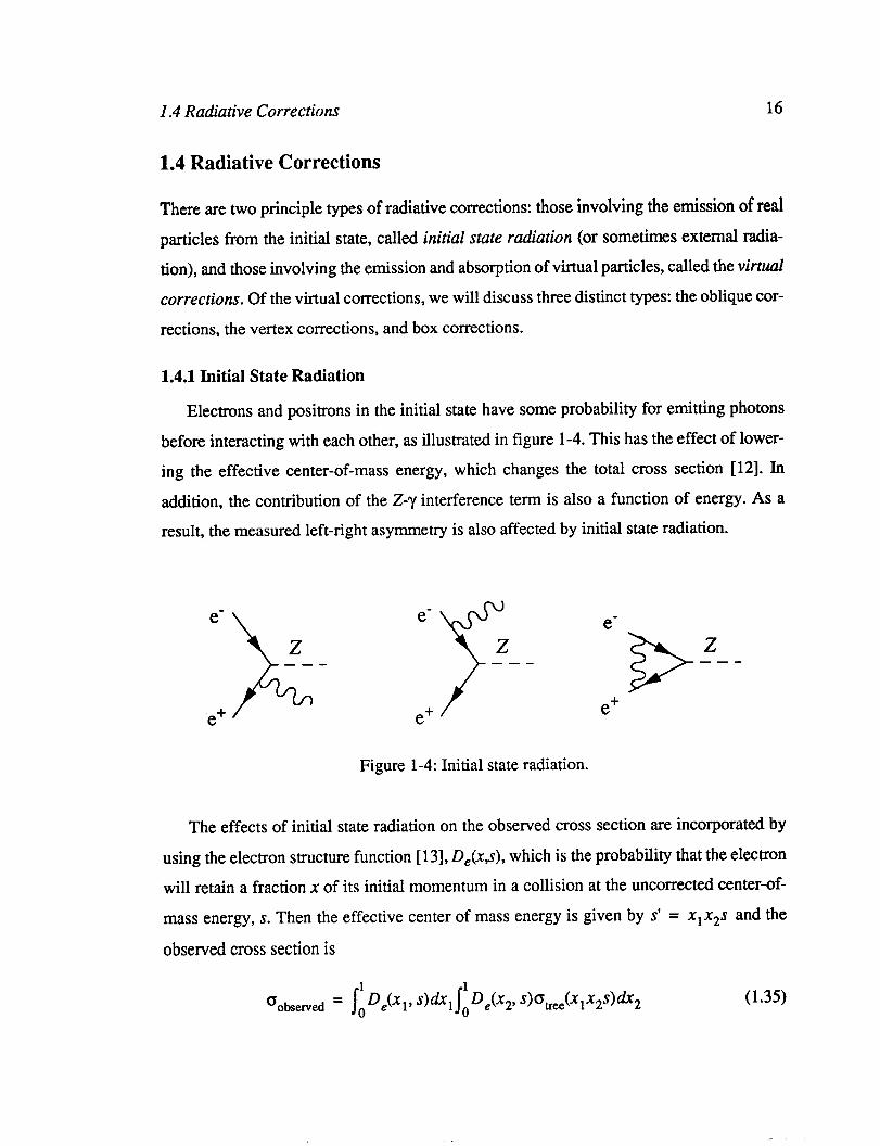
1.4.1 Initial State Radiation
Electrons and positrons in the initial state have some probability for emitting photons
before interacting with each other, as illustrated in figure l-4. This has the effect of lower-
ing the effective center-of-mass energy, which changes the total cross section [12]. In
addition, the contribution of the Z-y interference term is also a function of energy. As a result, the measured left-right asymmetry is also affected by initial state radiation.
e’ z
h
---
e+
e- z
F
---
e+
e-
c, z --- e+
Figure l-4: Initial state radiation.
The effects of initial state radiation on the observed cross section are incorporated by
using the electron structure function [ 131, D&S), which is the probability that the electron
will retain a fraction x of its initial momentum in a collision at the uncorrected center-of-
mass energy, S. Then the effective center of mass energy is given by s’ = x1x2s and the
observed cross section is
(1.35)

I .4 Radiative Corrections 17
At tree level, the function D,(x,s) was calculated by Bonneau and Martin [14], which
leads to a -29% correction to the tree-level cross section, shown in figure 1-5. Such a large
correction suggests that higher order terms are called for [ 151
where P = f
The effect of this correction is also shown in figure l-5.
b
3-m
0 I I I -
88 88 90 90 92 92 94 94 96 96 E E c.m. (GW c.m. (GW 6661A15 6661A15
Figure 1-5: Radiative corrections to the 2 peak cross section. Figure 1-5: Radiative corrections to the 2 peak cross section.
(1.36)
1.4.2 Oblique Corrections
Vacuum polarizations affect the interactions by modifying the gauge boson propagators
(and thereby the coupling constants). This is why they are referred to as oblique corrections,
as compared to the direct (vertex and box) corrections which modify the form of the inter-
.
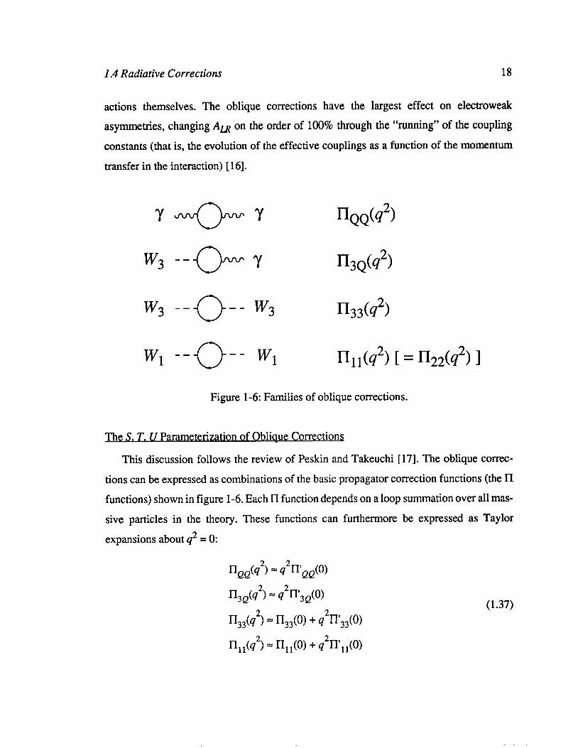
I .4 Radiative Corrections 18
actions themselves. The oblique corrections have the largest effect on electroweak
asymmetries, changing A,IJ on
constants (that is, the evolution
transfer in the interaction) [ 161.
Y
w3 -- 0 --
Wl -- 0 --
the order of 100% through the “running” of the coupling
of the effective couplings as a function of the momentum
Y nQQh2)
Y 2
&Q(q )
w3 H33(q2)
w1 n,,(92) [ = b2(q2) 1
Figure l-6: Families of oblique corrections.
The S, T. U Parameterization of Oblique Corrections
This discussion follows the review of Peskin and Takeuchi [17]. The oblique correc-
tions can be expressed as combinations of the basic propagator correction functions (the II
functions) shown in figure l-6. Each II function depends on a loop summation over all mas-
sive particles in the theory. These functions can furthermore be expressed as Taylor
expansions about q2 = 0:
(1.37)

I .4 Radiative Corrections 19
where II’ is equal to dWdq2 in these expressions. The QED Ward Identity assures that
II,,(O) = II3a(O) = 0. These expansions are valid only to the order of (mdmv>2, where
mN is the energy scale of any new physics phenomena.
Under this scheme the manifestations new physics through the oblique corrections are
encompassed by six parameters. Three independent precision measurements, listed in table l-2, fix three of these functions, leaving three undetermined parameters.
On their own, many of the II functions contain ultraviolet divergences. However, the
comparison of physical observables always involves the diference of these functions. It is
therefore reasonable to define the following independent combinations, which are all ultra-
violet finite, as the remaining three parameters in electroweak interactions:
s 4e2 = a W&O) - ~‘qp>l
TE 2 W,,(O) - I-@31 as c mz
u = g [rr,,(O) -n’,,(O)]
(1.38)
where s and c are the sine and cosine of the Weinberg angle.
Reference values of observables can be calculated for the Standard Model (that is, by
including only Standard Model particles), given an assumption of the top quark mass (m,)
and the Higgs mass (mH). It is then assumed that deviations from the model are the result of new heavy physics entering through small oblique corrections. Then the observable 0’
can be expressed as a Standard Model reference value expanded to first order in S, T and
U, that is
0’ = O’(m,, mH)lSlandard Model + a’S + b’T + c’U (1.39)
where the expansion coefficients a, b, and c are theoretically determined for each observ-
able. Note that these coefficients are independent of m, and mm A compilation of such
coefficients is found in Reference [ 171.
1.4 Radiative Corrections 20
A general system for testing the Standard Model through oblique corrections is avail-
able through the scheme described above. It is particularly easy to discuss the case of
neutral current observables (all those described in this chapter with the exception of the W
mass), which are independent of the Uparameter. Therefore, the measurement and error for a given neutral current observable defines a confidence band in S-T space, with a slope
equal to the ratio of the expansion coefficients, -ai/bi. The combination of measurements
with different expansion coefficients then defines a region in S-T space, which may be con-
sistent with the Standard Model (S = T = 0), or some non-zero values of S and T, which would be indicative of new physics. We will use this system to compare the SLD A, mea-
surement to the Standard Model in Chapter 5.
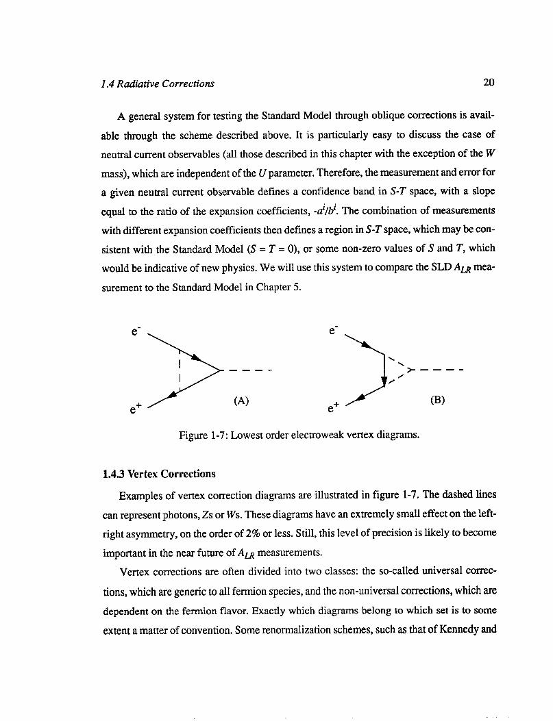
e-
e+ (4
e-
e+ (B)
Figure l-7: Lowest order electroweak vertex diagrams.
1.4.3 Vertex Corrections
Examples of vertex correction diagrams are illustrated in figure l-7. The dashed lines
can represent photons, Zs or Ws. These diagrams have an extremely small effect on the left-
right asymmetry, on the order of 2% or less. Still, this level of precision is likely to become
important in the near future of Am measurements. Vertex corrections are often divided into two classes: the so-called universal correc-
tions, which are generic to all fermion species, and the non-universal corrections, which are
dependent on the fermion flavor. Exactly which diagrams belong to which set is to some
extent a matter of convention. Some renormalization schemes, such as that of Kennedy and

I .5 Properties of ALR 21
Lynn [ 181, include a particular set of universal vertex corrections as well as oblique correc-
tions in the definition of the weak mixing angle, a point that is amplified in section 1.6.
Figure l-8: Lowest order electroweak box diagrams.
1.4.4 Box Corrections
Examples of box diagrams are illustrated in figure l-8. The dashed lines can represent
photons, 2s or Ws. Corrections to ALL arising from such diagrams are less than 0.5% and
are negligible in this analysis.
1.4.5 QCD Corrections
All of the corrections discussed so far arise from the electroweak sector. Corrections
arising from QCD effects are generally ignored. It has been shown that all QCD radiative
corrections to the left-right asymmetry are suppressed to all orders by at least one factor of
a [ 191. Such corrections are therefore at least an order of magnitude smaller than elec-
troweak corrections. Furthermore, effects arising from final state interactions and
fragmentation rigorously cancel in the asymmetry, up to the level of the box diagrams.
Even in box diagrams, QCD only enters in at the level of 10% (the factor of CXJ compared
to the electroweak corrections.
1.5 Properties of ALR
Now that we have discussed the necessary background, we describe how the left-right
asymmetry is measured experimentally, and discuss the advantages of the measurement.

I.5 Properties of ALR 22
In this section and throughout this document we will refer to the left-right asymmetry
of some quantity Q as AQ, defined by
A I (QL-QR>
Q (QL+QR> ww
where QL refers to the quantity Q associated with left-handed electrons, and QR refers to the quantity associated with right-handed electrons. For instance, the polarization asymme-
try is the difference between the polarization of left-handed (PL> and right-handed (PR)
electron bunches, normalized to the sum of those polarizations, and is denoted by Ap.
1.51 The Measured Left-Right Asymmetry
Given the form of the cross section in equation (1.23), the expected number of left-
handed 2 productions, NL, and the expected number of right-handed 2 productions, NR,
over some period of running, T, is
(1.41)
NR = ‘R%npj LR(t) [ 1 - P,(t)A,,l df 0
where E is the detection efficiency, a function of the detector acceptance assumed to be con-
stant in time. L is the luminosity, and P is the longitudinal electron polarization, both of
which change with time. The unpolarized cross section o,, is defined in equation (1.23).
If we assume that the AQ are zero, that is, EL = ER, LL = LR = L, and PL = PR = P,, it follows
from (1.41) that the measured number asymmetry, AN, is
(Nr, - NR> AN= (NL+NR) = (Pe)ALR (1.42)
1.5 Properties of ALA 23
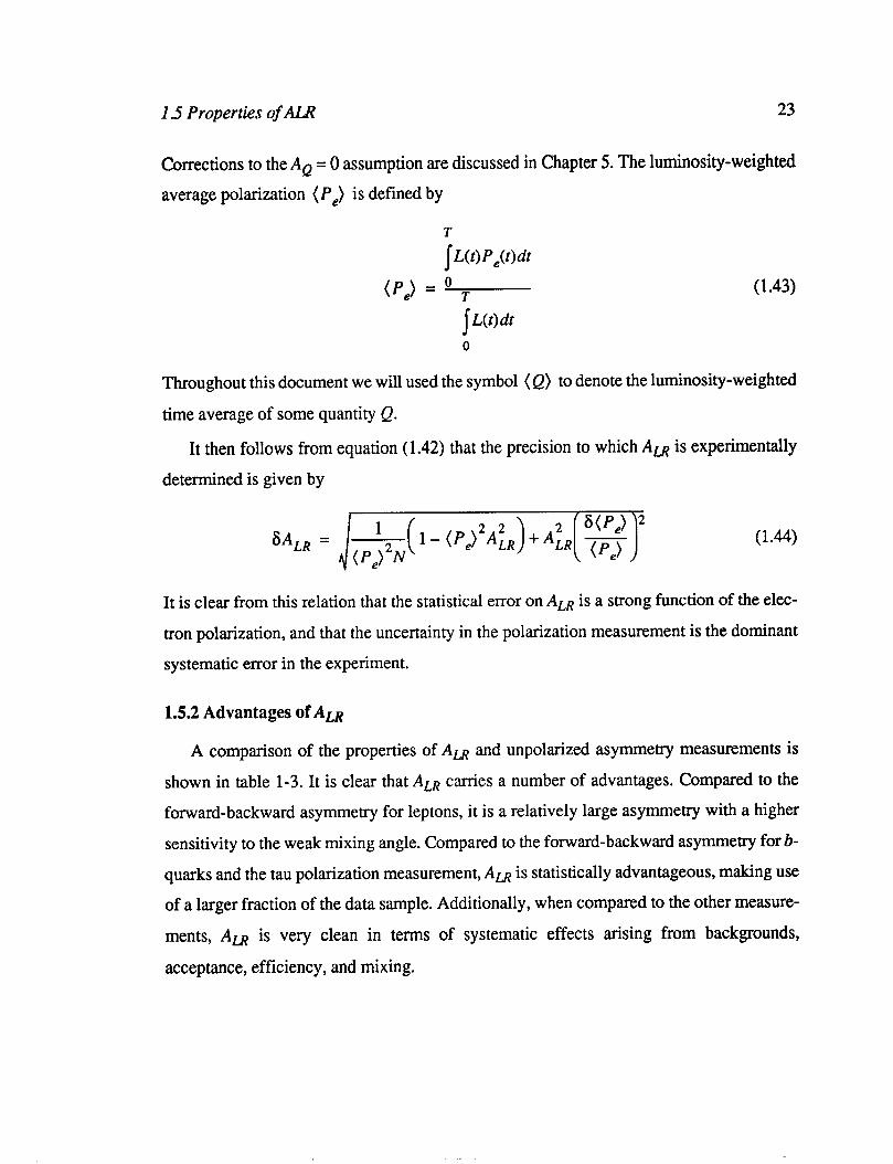
Corrections to the AQ - - 0 assumption are discussed in Chapter 5. The luminosity-weighted
average polarization (PJ is defined by
lp,> = ’ T
I L(t)dt
0
(1.43)
Throughout this document we will used the symbol (Q) to denote the luminosity-weighted
time average of some quantity Q.
It then follows from equation (1.42) that the precision to which Am is experimentally
determined is given by
6ALR = ’ “I (PJ2N
(’ - (pe)2Af,) + AiR (1.44
It is clear from this relation that the statistical error on A, is a strong function of the elec-
tron polarization, and that the uncertainty in the polarization measurement is the dominant
systematic error in the experiment.
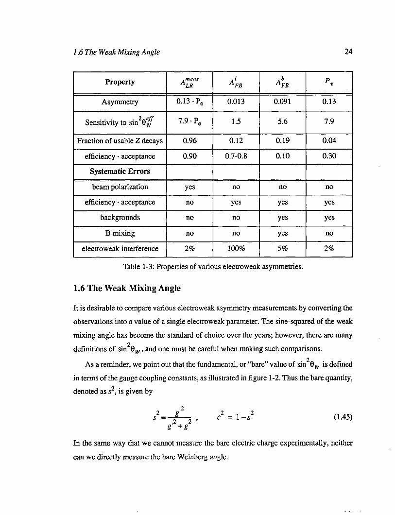
1.5.2 Advantages of ALR
A comparison of the properties of Am and unpolarized asymmetry measurements is
shown in table l-3. It is clear that ALR carries a number of advantages. Compared to the
forward-backward asymmetry for leptons, it is a relatively large asymmetry with a higher
sensitivity to the weak mixing angle. Compared to the forward-backward asymmetry for b-
quarks and the tau polarization measurement, Am is statistically advantageous, making use of a larger fraction of the data sample. Additionally, when compared to the other measure-
ments, Am is very clean in terms of systematic effects arising from backgrounds,
acceptance, efficiency, and mixing.
I .6 The Weak Mixing Angle 24
Table l-3: Properties of various electroweak asymmetries.
1.6 The Weak Mixing Angle
It is desirable to compare various electroweak asymmetry measurements by converting the
observations into a value of a single electroweak parameter. The sine-squared of the weak
mixing angle has become the standard of choice over the years; however, there are many
definitions of sin28 w, and one must be careful when making such comparisons.
As a reminder, we point out that the fundamental, or “bare” value of sin2C$+, is defined
in terms of the gauge coupling constants, as illustrated in figure 1-2. Thus the bare quantity,
denoted as s2, is given by
S2 g J
s-
gt2 + g2 , C2 = l-s2 (1.45)
In the same way that we cannot measure the bare electric charge experimentally, neither
can we directly measure the bare Weinberg angle.

I .6 The Weak Mixing Angle 25
It has been shown that the effects of the oblique corrections and a particularly defined
set of universal vertex corrections can be absorbed into the coupling constants and propa-
gators of the electroweak matrix elements, without altering the form of the interactions
themselves [18]. In this case, the neutral current Lagrangian is given by
L neutral = e,j?y’f A, - sff [ ( 1 - ys) T; - s:Q~] f 2, * * (1.46)
from which it follows that the left-right asymmetry, now corrected for all orders of vacuum polarization, is
A,&*) 2 [ 1 4&l*)]
-
= [ 1 - 4&s*)] * * 1 + (1.47)
This quantity is essentially what is directly measured by experiment, to within the small
non-universal vertex corrections and box corrections.
1.6.2 sz and ~3
One definition of the electroweak mixing angle in terms of measured quantities is sug-
gested by Sirlin [20]:
(1.48)
This quantity has the disadvantage in being related to the W mass, which is not one of the
best-measured electroweak parameters. The currently most precise measurement [21]
determines the Sirlin angle to be
S5 = 0.2256 f 0.0047 (1.49)

I .6 The Weak Mixing Angle 26
A more accurate determination of the mixing angle is suggested by [22]
(1.50)
where a*, is the running electromagnetic coupling, renormalized by oblique corrections to
the photon propagator, accounting only for known quarks and leptons. This value is calcu-
lated to be [23]
2 -1 a*,(mz) = 128.80 Z!I 0.12 (1.51)
which, when combined with the values given in table l-2, yields a value
St = 0.23135 +_ 0.00031 (1.52)
This extremely accurate reference value may now serve as a basis for detecting new heavy
physics through oblique radiative corrections. Of particular interest:
Standard Model
1.6.3 sin 2 eff 8,
(1.53)
The most logical choice of definition for experimentalists is the eflective weak mixing
angle, sin * eff The effective mixing angle is strictly defined at the 2 pole, such that 8, .
4R = ALR(mi) = 2 [ 1 - 4sin*$j
1 + [l-4sin*$~*
and
eff
sin * err=: 8, - - t 1 12cf at?
(1.55)

I .6 The Weak Mixing Angle 27
where the electron weak coupling constants v, and a, have been renormalized to the energy
scale of the Z mass to from effective coupling constants. The effective mixing angle implic-
itly includes the oblique corrections and universal vertex corrections, as well as the non-
universal electron vertex corrections. The effects of initial state radiation are not and cannot
be included in a general definition, because they depend on detector acceptance. Therefore
each experiment must account for initial state radiation, and the electroweak interference
that accompanies a real measurement away from the Z pole, when converting an observa- 2 eff tion into a value of sin 8, .
The relationship between the effective mixing angle and other mixing angle definitions
is made explicit in the following equations:
sin 8, * eff = (1 + AK,) st(rni)
(1.56)
where AK, is the weak form factor associated with the electron/positron vertex which
parameterizes the difference between st and sin * eff. This form factor is calculated to 8,
have a Standard Model value of AK, = 0.0226 [24]. It can be further broken down into uni-
versal and non-universal parts, Atcuniv and Av?‘~~-~~“. As discussed in the previous section,
the universal part is absorbed into the definition of s* * . The remaining non-universal part is
small, with a calculated Standard Model value of AK”on-u”iv = 0.003 [25]. Hence the value 2 eff of sin 8, is substantially different from that of ~5 but very close to that of s:.
1.6.4 Converting to the Weinberg Angle
The machinery used to convert a measurement of Am into sin*8: is the software
package ZFITTER [24]. The result of many man-years of effort, ZFIITER is a flexible pro-
gram that calculates Standard Model cross sections and asymmetries by various methods.
The primary method employs analytic formulae with higher order corrections, including
the oblique, vertex, and box diagram corrections discussed above, to first order. This is the

I .7 Thesis Outline 28
method used for the Standard Model fits presented in this document. Other methods use
model-independent approaches based on effective couplings or partial decay widths.
In addition, ZFITIER includes the effects of initial state radiation, either employing no
cuts on the bremsstrahlung photon phase space, or a cut on the maximum allowed energy of a bremsstrahlung photon, or simultaneous cuts on the energy and acollinearity of the
final state fermions.
1.7 Thesis Outline
The remainder of this thesis deals with the experimental aspects of the Aa measurement.
Chapter 2 describes the hardware necessary to create, transport, and collide polarized
electrons and positrons, as well as the hardware components of the Moller and Compton
polarimeters and the SLD detector. Chapter 3 concentrates the details of Compton scattering kinematics, the Compton
polarimeter analysis and associated systematic errors, and presents the resulting average
luminosity-weighted polarization.
Chapter 4 describes the analysis of SLD data, the event selection criteria, and the back-
ground estimation, and gives the result for the measured Z asymmetry.
Chapter 5 discusses the corrections to the measured polarizations and asymmetries (in
particular the chromaticity correction) and the various systematic cross-checks that were
made, and gives the result for Am and the associated estimate of systematic errors. This
result is then converted into a measurement of sin*8: and compared to other experiments
and the Standard Model.
Chapter 2
Experimental Apparatus
Given the definition of Am, it is clear that we require certain experimental apparatus in
order to carry out the measurement, specifically:
l A source of polarized electrons
l An electron accelerator and spin transporter l A beam polarization monitor
l A Z boson detector
The fulfillment of these requirements is met in turn by the SLAC Linear Collider (SLC),
the Moller and Compton polarimeters, and the SLD detector. The hardware components
and general operation of the SLC, the SLD detector, and the polarimeters are the subjects
of this chapter.
2.1 The Polarized SLC
The SLAC Linear Collider is the world’s first linear e+e’ collider, producing head-on
collisions of electrons and positrons accelerated in the SLAC linear accelerator (or Zinuc).
These collisions result in the production of massive resonant particles such as the Z boson.
The SLC is also the first and only accelerator to produce 2 bosons with polarized electron beams [26].
29
2.1 The Polarized SLC 30
Compton Polarimeter
Linac -’ Moller 4 Polarimeterx
e- Spin Vertical-“’ Linac
e+ Source
-$1 e+ Return Line
e- Damping e+ Damping Ring
Electron Spin Direction Polarized e- Source
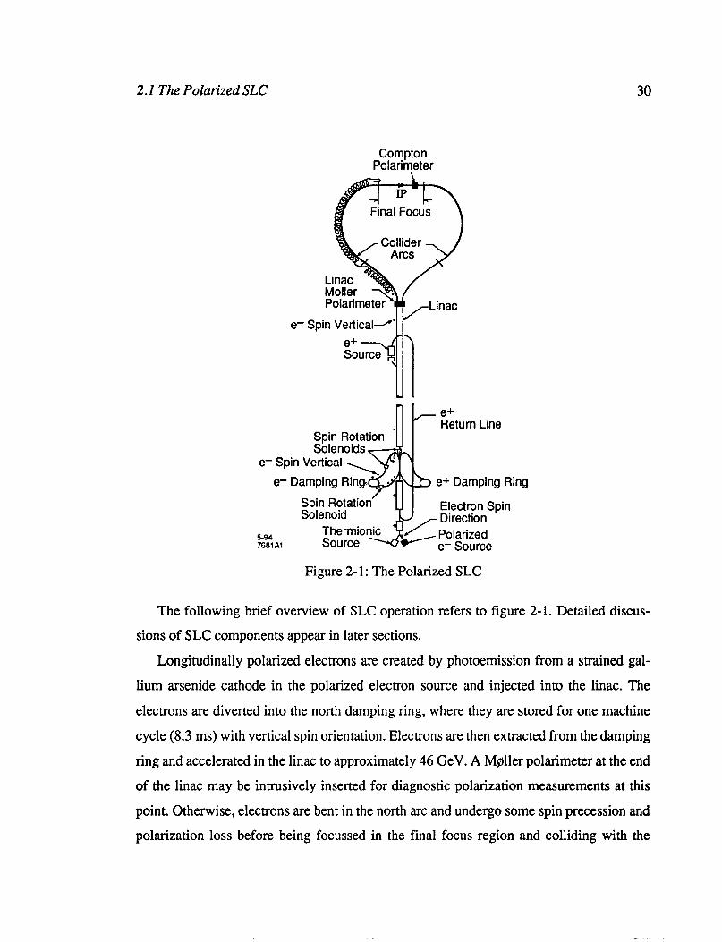
Figure 2- 1: The Polarized SLC
The following brief overview of SLC operation refers to figure 2- 1. Detailed discus-
sions of SLC components appear in later sections.
Longitudinally polarized electrons are created by photoemission from a strained gal-
lium arsenide cathode in the polarized electron source and injected into the linac. The
electrons are diverted into the north damping ring, where they are stored for one machine
cycle (8.3 ms) with vertical spin orientation. Electrons are then extracted from the damping
ring and accelerated in the linac to approximately 46 GeV. A Moller polarimeter at the end
of the linac may be intrusively inserted for diagnostic polarization measurements at this
point. Otherwise, electrons are bent in the north arc and undergo some spin precession and polarization loss before being focussed in the final focus region and colliding with the

2.1 The Polarized SLC 31
positron bunch at the SLD interaction point. Collision products are measured by the SLD
detector. The electron bunch then continues past the interaction point and collides with the
Compton polarimeter polarized target. The products from this collision are scattered in to
the Compton Cherenkov detector, which provides a continuous monitor of the longitudinal
electron polarization. The main electron bunch continues down the arc, where it finally
encounters the energy spectrometer magnets before entering the electron dump. Synchro-
tron photons from the spectrometer magnets are detected in the Wire Imaging Synchrotmn
Radiation Detector, which provides a continuous precision beam energy measurement.
2.1.1 Polarized Electron Source
Polarized electron beams have been in use at SLAC since the spring of 1992. The SLAC
Linear Collider injector requires that two 2 ns pulses of 4.5-5.5~10’~ electrons, separated
by 61 ns, to be produced at 120 Hz [27]. These specifications are met by the Polarized Elec-
tron Source (PES), which consists of a diode-type electron gun in which electrons are
extracted from a gallium-arsenide photocathode by a laser operating near the semiconduc-
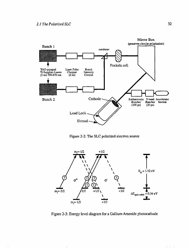
tor band gap energy. A schematic representation of the PES is shown in figure 2-2. A
discussion of the main PES components follows.
Gallium-Arsenide (GaAs) Photocathodes
It has been long known that polarized electrons can be extracted by photoemission from
a semiconductor surface [28]. Figure 2-3 shows an energy level diagram for gallium-ars-
enide. The solid lines indicate transitions induced by right-handed photons and the dotted
lines indicate transitions induced by left-handed photons. The numbers in circles are the
relative Clebsh-Gordon coefficients for each transition.
From this diagram, we see that photons with an energy 1.52 eV 5 E,,< 1.86 eV only
excite transitions from the Pjl, level of the valence band. If we further assume that the pho-
tons are right-handed (that is to say, they have positive helicity, or their angular momentum
and momentum are parallel), only two transitions are possible: the P state with m. = -3/2
can make a transition to the S state with mj = -l/2, and the P state with mj = -l/2 can make
a transition to the S state with mi = +1/2. The former transition ejects an electron with spin
2.1 The Polarized SLC 32
Mirror Box (preserves circular polr
I Bunch 1 ization)
I Pockels cell \ Ti: S apphiie Lasers (3 ns) 750-870 nm
Bunch 2
Figure 2-2: The SLC polarized electron source
m;=-l/2 +I/2
IIlj=- l/2 +1/2
\ \
\ 3 Q
E, = 1.52 eV
Figure 2-3: Energy level diagram for a Gallium Arsenide photocathode

2.1 The Polarized SLC 33
antiparallel to the incident photon direction (that is, parallel to its ejected momentum, or right-handed), and has a probability three times greater than the latter transition, which
ejects left-handed electrons. In other words, the absorption of right-handed photons pro-
duces a preferentially right-handed electron bunch, with a maximum polarization given by
P 3-l max = - = 50% 3+1 (2.1)
The symmetry of the energy levels shows that left-handed photons produces a bunch of left-
handed electrons with the same polarization.
Of course, all that has been shown at this point the that we can create polarized electrons
in the conduction band of GaAs. In normal GaAs, the energy gap between the conduction
band and the free electron state (referred to as the work function of the material) is on the
order of 2.5 eV, and even under the large electric fields applied in the gun, pure GaAs is a
poor photoemitter. Photoemission quality is quantified by the quantum eficiency or QE of a material,
which is the probability that an electron will be emitted when a photon is incident on the
material surface.
It turns out that a surface application of cesium serves to bring the work function to zero
or even negative, vastly increasing the QE of the cathode. During normal source operation,
in order to activate the highest quantum efficiency, the cathode is heated to 610 OC for one
hour, cooled to room temperature, and then treated with Cs until the photocurrent peaks.
To fix the cycle, the cathode is treated with a codeposition of Cs and NF3.
We have seen that in normal Gallium arsenide, the energy degeneracy in the P3,2 level
makes 50% the theoretical upper maximum achievable polarization. If there were some
way to break this degeneracy, then the theoretical maximum polarization would be 100%.
It turns out that the use of a strained lattice cathode, added to the polarized source in 1993
and one of the keys to the success of the run, does just that.
2.1 The Polarized SLC 34
Strained GaAs Cathodes
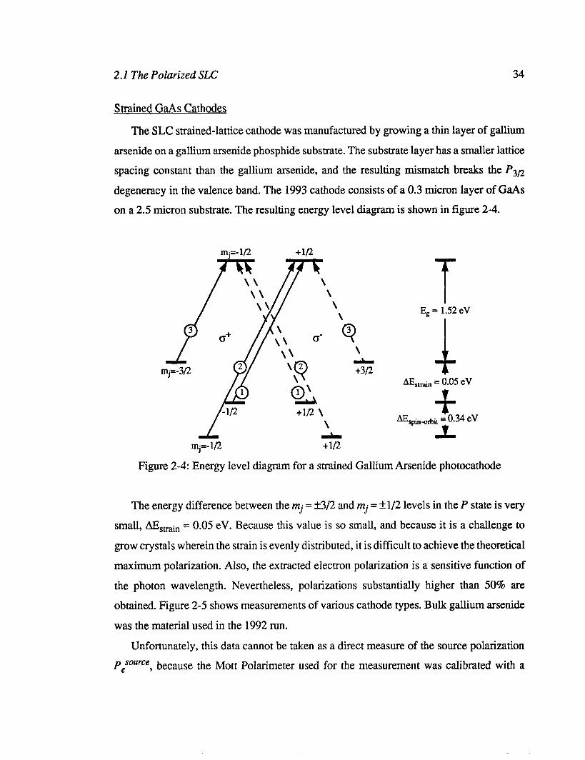
The SLC strained-lattice cathode was manufactured by growing a thin layer of gallium
arsenide on a gallium arsenide phosphide substrate. The substrate layer has a smaller lattice
spacing constant than the gallium arsenide, and the resulting mismatch breaks the P3n
degeneracy in the valence band. The 1993 cathode consists of a 0.3 micron layer of GaAs on a 2.5 micron substrate. The resulting energy level diagram is shown in figure 2-4.
mj=-l/2 +1/2
Eg = 1.52 eV
AEsth = 0.05 eV
t AEsp,**it=O.34 eV
L
Figure 2-4: Energy level diagram for a strained Gallium Arsenide photocathode
The energy difference between the mj = f3/2 and mj = &l/2 levels in the P state is very
small, AE,,h = 0.05 eV. Because this value is so small, and because it is a challenge to
grow crystals wherein the strain is evenly distributed, it is difficult to achieve the theoretical
maximum polarization. Also, the extracted electron polarization is a sensitive function of
the photon wavelength. Nevertheless, polarizations substantially higher than 50% are
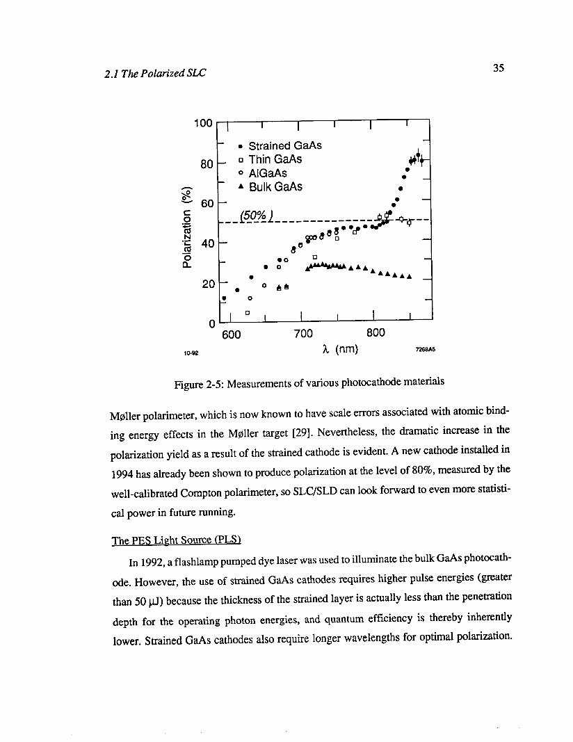
obtained. Figure 2-5 shows measurements of various cathode types. Bulk gallium arsenide
was the material used in the 1992 run.
Unfortunately, this data cannot be taken as a direct measure of the source polarization
P ‘Ource, e because the Mott Polarimeter used for the measurement was calibrated with a
2.1 The Polarized SLC 35
l Strained GaAs 0 Thin GaAs 0 AlGaAs * Bulk GaAs
0 I I I I I 600 700 800
lo-92 h (nm) 725SA5
Figure 2-5: Measurements of various photocathode materials
Moller polarimeter, which is now known to have scale errors associated with atomic bind-
ing energy effects in the Moller target [29]. Nevertheless, the dramatic increase in the
polarization yield as a result of the strained cathode is evident. A new cathode installed in
1994 has already been shown to produce polarization at the level of 80%, measured by the
well-calibrated Compton polarimeter, so SLCXLD can look forward to even more statisti-
cal power in future running.
The PES Light Source (PLSl
In 1992, a flashlamp pumped dye laser was used to illuminate the bulk GaAs photocath-
ode. However, the use of strained GaAs cathodes requires higher pulse energies (greater
than 50 ClJ) because the thickness of the strained layer is actually less than the penetration
depth for the operating photon energies, and quantum efficiency is thereby inherently
lower. Strained GaAs cathodes also require longer wavelengths for optimal polarization.

2 .I The Polarized SLC 36
Referring to figures 2-3 and 2-4 we see that a bulk GaAs can be illuminated by energies as
high as 1.86 eV, or wavelengths as short as 667 nm, whereas strained GaAs cannot go
higher than 1.57 eV, or lower than 790 nm. There were in fact no commercial lasers avail-
able with the required specifications, so the necessary system was developed at SLAC. The only commercially available solid state laser material which operates over the
required wavelength range at the required power and repetition rate is titanium-doped sap-
phire (TI+3:AlZ03), and the 1993 PLS was designed around this material. Two Ti-sapphire
resonant cavities, each operating at 120 Hz, are both pumped by two frequency doubled Nd:YAG lasers, each operating at 60 Hz. The first Ti-sapphire laser runs is at 864 nm as
extracts electrons for collision. The second runs at 707 nm and extracts electrons for the
positron source. A complex feedback system reduces the output jitter of the lasers to less
than 3% RMS [27].
Both beams pass through the circularly polarizing Pockels cell at the same voltage set-
ting. A Pockels cell consists of a KD*P’ crystal sandwiched between two plates that
generate an electric field along the longitudinal (or z) axis of the crystal. When light passes
through the crystal, a phase shift is generated between field components projected along the
fast (x) axis and the slow (y) axis. This phase shift is proportional to the voltage applied to
the plates. Thus the Pockels cell acts as a variable phase shift generator. A given Pockels
cell has a unique voltage at which it operates as a quarter wave plate, called the quarter-
wave voltage (QWV), for a given frequency of light. When +QWV is applied to the source
Pockels cell, the source laser is circularly polarized with one handedness. When -QWV is
applied to the cell, the source laser is circularly polarized with the opposite handedness
(which handedness is created depends on the cell alignment and must be calibrated
experimentally).
The sign of the source Pockels cell QWV is chosen randomly on a pulse-by-pulse basis,
which controls the helicity of the source laser, which in turn controls the helicity of the
extracted electrons. Thus the helicity of the beam pulse is chosen randomly, and this infor-
mation is transmitted and incorporated into the SLD data acquisition. The helicity bits are
1. Potassium Dideuterium Phosphate

2 .I The Polarized SLC 37
transmitted on three redundant systems: the KVM (Klystron Veto Module) system, the
Mach line (direct signal wires from the PLS to SLD), and the PMON (Polarization MON-
itor) system. The helicity bit transmission has been rigorously tested (see section 5.3).
Higher currents are required in the second electron bunch, in order to extract enough positrons from the positron source to match the first electron bunch. For this reason the sec-
ond Ti-sapphire laser operates at a lower wavelength, in order to increase the quantum
efficiency and avoid the charge limit effect (see below). Therefore, the nth machine pulse
(and nth PLS Pockels cell voltage setting) has two electron pulses associated with it, a polarized bunch for collisions, and a bunch for the positron source, with a low but unknown
polarization. Here is the important point: even if the second electron bunch retains some
polarization information, and if this information were somehow imparted to the positrons
created by this bunch, this would still have no effect on the Au experiment. This is because
the positrons extracted by the nth unpolarized electron bunch are used to collide with the
(n+l)th polarized electron bunch whose polarization state is completely uncorrelated with the nth bunch (since the polarization of any bunch is chosen randomly). Therefore, any
effect stemming from residual positron polarization of this type rigorously vanishes when
averaged over time.
The Electron Gun
The SLC polarized electron gun, shown in figure 2-6, employs a conventional diode
design. During operation, the cathode potential is -120 kV, which draws a space-charge
limited current of 8.9 amperes, or 1.1~10” electrons in a 2 ns bunch. However, as dis-
cussed in the next section, this is not the limiting factor on current from the PES.
The high voltage end of the gun is connected to the so-called load lock, which allows a
new photocathode to be installed in the gun without affecting the gun’s ultra-high vacuum
[30]. The load lock system provides three major advantages over the previous system. First,
without the load lock system, the gun must be brought to atmosphere in order to change
cathodes, and then re-baked each time with the cathode in place. This degrades both the
high voltage performance of the gun and the quantum efficiency of the cathode. The second
advantage of the load lock system is that the time required to load a new photocathode is

2 .I The Polarized SLC 38
Polarized Gun II
Figure 2-6: The SLC Polarized Electron Gun
reduced from three weeks to a matter of hours. Finally, the cathode is easily removed for
high voltage processing of the gun electrodes.
The Charge Limit
For low source laser currents, the number of electrons extracted from the source is pro-
portional to the laser pulse energy. However, the dependence becomes strongly non-linear
at higher wavelengths and pulse energies, and the number of extracted electrons eventually
saturates around 7x10” electrons per pulse. This number is well below the inherent space
charge limit of the gun, which is estimated at 1.1~10~’ electrons per pulse [31]. The exact cause of the charge limit effect has yet to be determined, although it is
hypothesized to be a result of charge trapping at the cathode surface. However, the effect
carries a hidden advantage: by operating in the charge limit regime of the photocathode
response, effects arising from intensity jitter in the electron beam are minimized.
2.1 The Polarized SLC 39
2.1.2 Flat Beam Operation
The SLC was designed to operate with round beams, in which the horizontal and verti-
cal beam emittance are equal (E, = E$. This mode of operation facilitates optical matching
in beam lines with cross-plane coupling elements such as the solenoidal spin rotator mag-
nets and the SLC arcs. However, storage rings naturally produce flat beams, in which E, >>
E,,, and the collision of flat beams produces higher luminosity.
Tests in 1992 demonstrated the technical feasibility of flat beam operation in the SLC
[32]. A number of new accelerator techniques were required [33], not the least of which
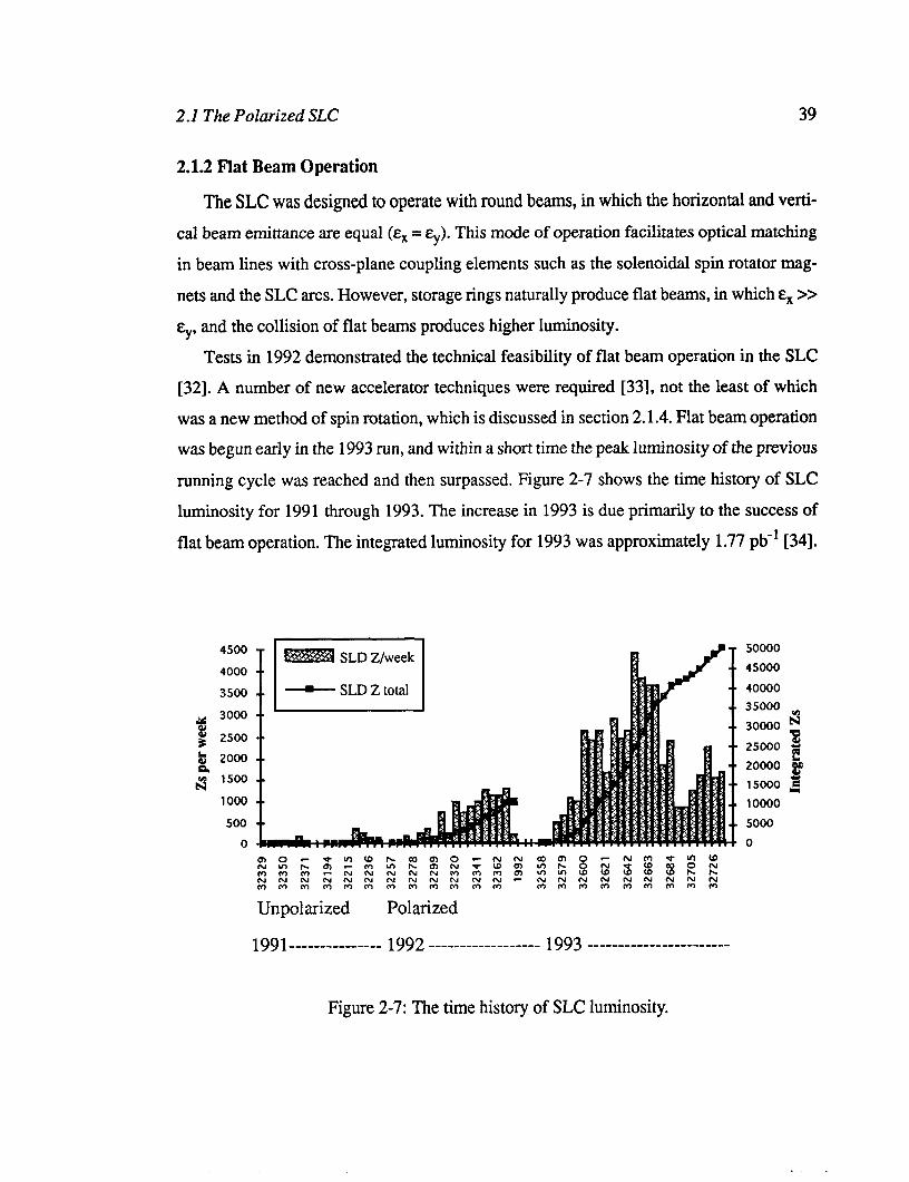
was a new method of spin rotation, which is discussed in section 2.1.4. Flat beam operation was begun early in the 1993 run, and within a short time the peak luminosity of the previous
running cycle was reached and then surpassed. Figure 2-7 shows the time history of SLC
luminosity for 1991 through 1993. The increase in 1993 is due primarily to the success of
flat beam operation. The integrated luminosity for 1993 was approximately 1.77 pb-’ [34].
4500 50000
4000 45000
3500 - SLD Z total 40000 35000
t 3000 2500 30000 A
25000 F k 2000 $ 20000
gJ
8 1500 15000 g 1000 10000
500 5000
0 0
1gg1__-----_____-__ 1992 ___.._____-____---_ 1993 __---__----------------
Figure 2-7: The time history of SLC luminosity.
2.1 The Polarized SLC 40
2.1.3 Spin Dynamics
It is of course not sufficient merely to have a source of polarized electrons. We also
require a method of maintaining and manipulating the spin in the accelerator. In order to
describe spin transport in the SLC, we must first discuss some general principles of electron
spin dynamics.
The precession of electron spins in magnetic fields is described fully by the BMT equa-
tions [35]. In the limit of planar motion through transverse magnetic fields, the spin
precession angle of the electrons, 8,, is directly related to the momentum precession angle
of the electrons, 8b, by the following equation
0, = y ( 1 9 8, (2.2)
where (g-2)/2 = 1.163x1 Om3 is the anomalous magnetic moment of the electron, and y is the
Lorentz factor, which is equal to Eb / m, in the limit of large beam energy, Eb The combi-
nation of these two coefficients is known as the spin tune, (v) which has a value on the order
of 100 at the full SLC energy.
In the case of solenoidal magnetic fields, the spin precession angle is given by
e _ eL(i;x3) s- m,cY
(2.3)
where L is the length of the magnet, B is the solenoidal field strength and 3 is the spin direc-
tion unit vector. Note that a solenoidal field precesses only transverse spin components.
2.1.4 Spin Transport
The main experimental goal regarding spin transport in the SLC is to maximize the lon-
gitudinal polarization at the SLD interaction point. This translates into three SLC
operational goals. First, spins must be oriented vertically in the North Damping Ring in
order to prevent loss of polarization. Second, spin orientation must be controlled at the IP.
Finally, spin diffusion (defined below) in the North Arc must be minimized.
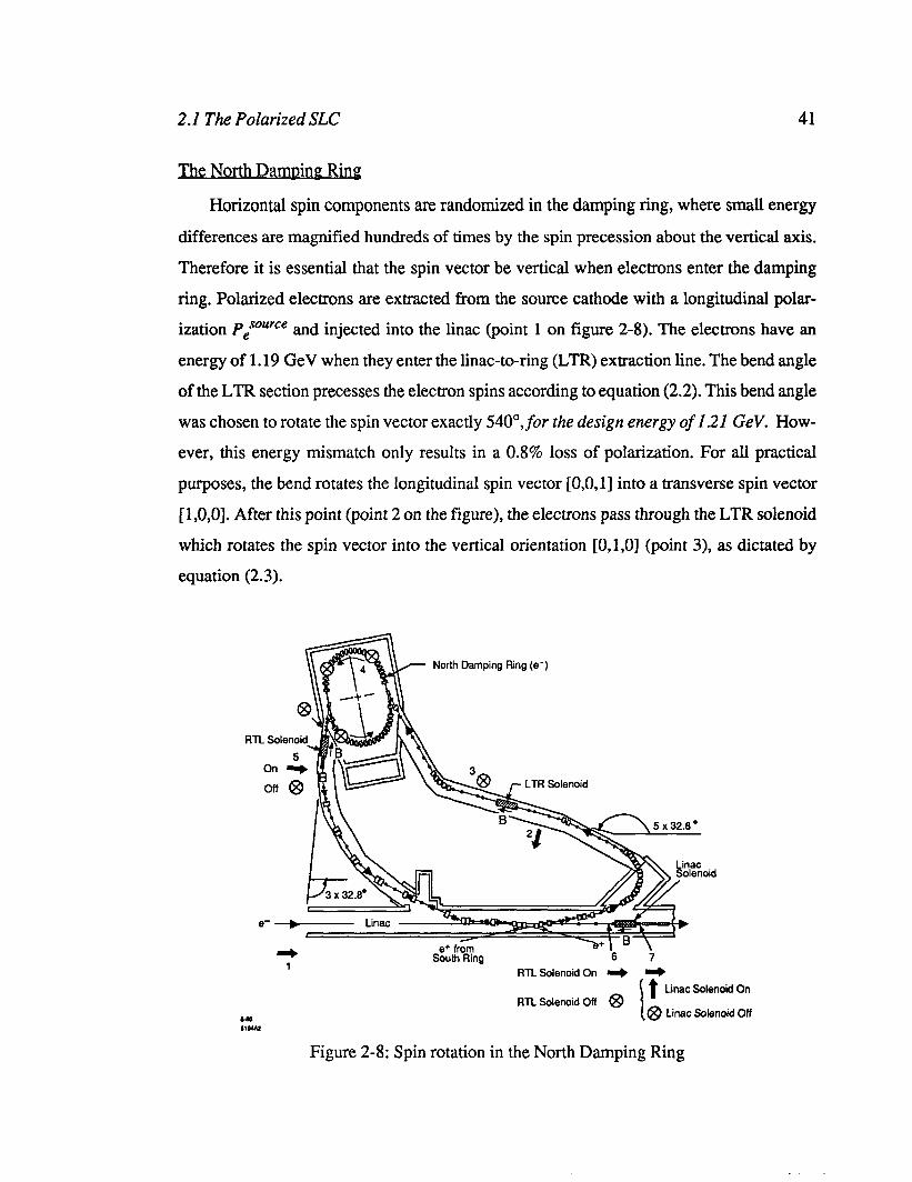
2 .I The Polarized SLC 41
The North Damning Ring
Horizontal spin components are randomized in the damping ring, where small energy
differences are magnified hundreds of times by the spin precession about the vertical axis.
Therefore it is essential that the spin vector be vertical when electrons enter the damping
ring. Polarized electrons are extracted from the source cathode with a longitudinal polar- ization P,“““” and injected into the linac (point 1 on figure 2-8). The electrons have an
energy of 1.19 GeV when they enter the linac-to-ring (LTR) extraction line. The bend angle
of the LTR section precesses the electron spins according to equation (2.2). This bend angle
was chosen to rotate the spin vector exactly 540”,for the design energy of I.21 GeV. How-
ever, this energy mismatch only results in a 0.8% loss of polarization. For all practical
purposes, the bend rotates the longitudinal spin vector [O,O,l] into a transverse spin vector
[ l,O,O]. After this point (point 2 on the figure), the electrons pass through the LTR solenoid
which rotates the spin vector into the vertical orientation [O,l,O] (point 3), as dictated by
equation (2.3).
North Damping Ring (e-)
LTR Solenoid
e+ from South Ring 6 7
e- - Linac I-
RTL Solenoid On I) r+
t Linac Solenoid On
RTL Solenoid Off @ @ Linac Solenoid Off
Figure 2-8: Spin rotation in the North Damping Ring

2.1 The Polarized SLC 42
After being cooled (cooling is the process of reducing the energy spread of the electron
bunch through synchrotron radiation damping) for 8.3 ms, the electrons are extracted from
the damping ring with the flat beam profile (E, = 9~~) and accelerated down the linac to
their full energy (46 GeV). The RTL and linac solenoids are turned off during normal run-
ning, in order to avoid rotating the flat beam profile, and the spin vectors remain in the
vertical orientation. At the end of the linac, the bunch has a transverse polarization denoted
by P;-, which differs from P,sowce by less than 1.0%.
Soin Rotation
A spin rotation system is required to manipulate the spin orientation from vertical at the
end of the linac to longitudinal at the IP. A general spin rotation system must induce con-
trolled rotations about two orthogonal axes. One possible implementation of such a system
is shown in figure 2-9.
I I
[Tl *
90’ spin
General Suin Transport
Interaction Point
the longitudinal axis
Figure 2-9: General spin rotation system
The purpose of the general spin rotation system is to set the spin vector at the interaction
point, SIP, equal to (O,O,l), that is, to a purely longitudinal spin state. This involves setting
the spin at some point in the machine, SG, such that the spin precession in the rest of the
machine, characterized by the transport matrix T, produces the desired SF If one can make
two arbitrary rotations about two orthogonal axes, one can satisfy this relation T.SG =
(O,O,l) for an arbitrary T. The first element of the general spin rotator makes one arbitrary
rotation. Then, after allowing normal spin transport to induce a 90’ spin phase advance and
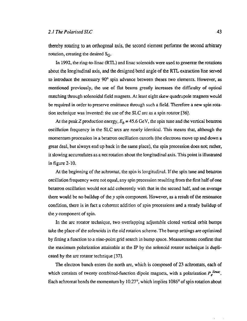
2.1 The Polarized SLC 43
thereby rotating to an orthogonal axis, the second element performs the second arbitrary rotation, creating the desired S,.
In 1992, the ring-to-linac (RTL) and linac solenoids were used to generate the rotations
about the longitudinal axis, and the designed bend angle of the RTL extraction line served
to introduce the necessary 90’ spin advance between theses two elements. However, as
mentioned previously, the use of flat beams greatly increases the difficulty of optical
matching through solenoidal field magnets. At least eight skew quadrupole magnets would
be required in order to preserve emittance through such a field. Therefore a new spin rota- tion technique was invented: the use of the SLC arc as a spin rotator [36].
At the peak 2 production energy, Eb = 45.6 GeV, the spin tune and the vertical betatron oscillation frequency in the SLC arcs are nearly identical. This means that, although the
momentum procession in a betatron oscillation cancels (the electrons move up and down a
great deal, but always end up back in the same place), the spin precession does not; rather,
it slowing accumulates as a net rotation about the longitudinal axis. This point is illustrated
in figure 2- 10.
At the beginning of the achromat, the spin is longitudinal. If the spin tune and betatron
oscillation frequency were not equal, any spin precession resulting from the first half of one
betatron oscillation would not add coherently with that in the second half, and on average
there would be no buildup of the y spin component. However, as a result of the resonance
condition, there is in fact a coherent addition of spin precessions and a steady buildup of
the y component of spin.
In the arc rotator technique, two overlapping adjustable closed vertical orbit bumps
take the place of the solenoids in the old rotation scheme. The bump settings are optimized
by fitting a function to a nine-point grid search in bump space. Measurements confum that the maximum polarization attainable at the IP by the solenoid rotator technique is dupli-
cated by the arc rotator technique [37].
The electron bunch enters the north arc, which is composed of 23 achromats, each of
which consists of twenty combined-function dipole magnets, with a polarization Pelinac.
Each achromat bends the momentum by 10.27’, which implies 1086” of spin rotation about
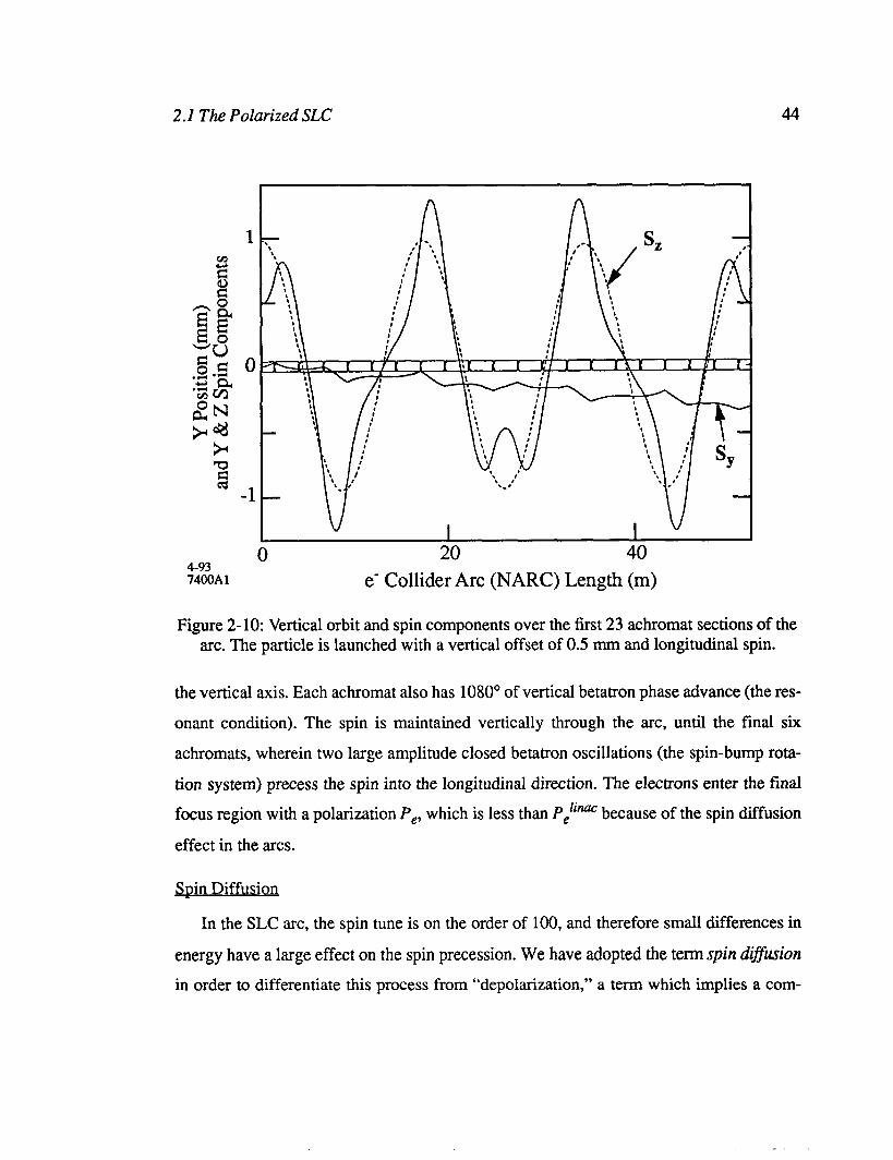
2.1 The Polarized SLC
4-93 7400A 1 e-
20 Collider Arc (NARC) Length
40
(ml
Figure 2-10: Vertical orbit and spin components over the first 23 achromat sections of the arc. The particle is launched with a vertical offset of 0.5 mm and longitudinal spin.
the vertical axis. Each achromat also has 1080’ of vertical betatron phase advance (the res-
onant condition). The spin is maintained vertically through the arc, until the final six
achromats, wherein two large amplitude closed betatron oscillations (the spin-bump rota-
tion system) precess the spin into the longitudinal direction. The electrons enter the final focus region with a polarization P,, which is less than P,lim because of the spin diffusion
effect in the arcs.
Snin Diffusion
In the SLC arc, the spin tune is on the order of 100, and therefore small differences in
energy have a large effect on the spin precession, We have adopted the term spin diflwion
in order to differentiate this process from “depolarization,” a term which implies a com-

2.1 The Polarized SLC 45
plete loss of polarization information. Polarization is not irretrievably lost during spin diffusion, as we will illustrate in the following example:
Suppose the SLC electron arc consisted of perfectly uniform positive and negative ver-
tical magnetic fields, and that the electrons are 100% longitudinally polarized. In the first section of the arc (the reverse-bend), the electron momentum is rotated exactly n/2 radians.
Following equation (2.2), the spin precesses approximately 26 times. However, the beam
has some energy spread, typically 0.2% RMS, and off-energy electrons will have different
precession angles. The precession angle is correlated with the energy except for the small
effect of synchrotron radiation induced randomization. The precession difference A.8 is
approximated by: A0 = v @E/E) = 0.21 radians. Thus the polarization of the beam at this
point is about 98%. After the second section of the arc, the central electrons are again
rotated 1t/2 radians, in the opposite direction. The polarization at this point is again lOO%!
The spin diffusion has been cancelled by an equal and opposite momentum precession, and
in this sense polarization is not truly lost. Diffusion occurs again through the final section
of the arc, leaving P, = 0.98.P,1imc.
Of course, the real SLC arc is not quite so simple. The arc is not perfectly planar, and the spin, which starts vertically, precesses about all three axes in a non-commuting manner.
Fortunately, we directly measure the dependence of spin on energy through experiments
with very low energy spread beams, where AE/E < 0.1%. Generation of such narrow energy
spreads requires low current running (=lO” e-/pulse) that is not suitable for normal physics
operation. A special machine experiment was run [37], during which the central energy of
the nearly monoenergetic beam was scanned, and polarization dependence on energy was
measured by the Compton polarimeter. Results from this experiment are shown in figure
2- 11 .The data were fit to the function
Pi = P;. cos 2xN. (2.4)
where PiZ is the measured polarization and Ei the measured energy of the ith scan point, PZc
was the optimized polarization measured by the Compton polarimeter at the nominal
2.2 h@ller Polarimetry 46
energy, E,, and N is the effective number of spin rotations in the arc x-z plane. The fit
results give N = 17.9 f 0.4, an number smaller than the 26 rotations predicted by the simple
planar model, as expected, since the spin has a significant vertical component throughout
the arc. This mode of operation has the advantage of lowering spin diffusion loss and also
reducing the polarization-energy correlation, an important property which is discussed fur-
ther in chapter 5. The loss of polarization due to spin diffusion is approximately 1.4% for a Gaussian energy spread of 0.15%.
0.7
Energy Offset @I.+‘)
Figure 2-l 1: The dependence of polarization on energy
2.2 Mplller Polarimetry
In the ALR experiment, it is of course necessary to monitor the polarization of the electron
beam. There are two methods employed to do this, both taking advantage of spin-dependent
QED cross-sections. One method is Mflller (electron-electron) scattering, and the other is
Compton (electron-photon) scattering. Each system requires a polarized target and a detec-
tor for the scattering products. The combination of target, detector, and data acquisition
system is referred to as a Polarimeter.
Moller polarimetry is based on the scattering of electrons off of polarized atomic elec-
trons in a magnetized target [38]. In the case where the center-of-mass energy of the two
2.2 Mdller Polarimetry 47
electron system, S, is much greater than the electron mass squared, the tree-level cross sec- tion for the scattering process in the center-of-mass frame is given by
_ cg( 3+cos20)2 do dS2 s sin48
[ 1 - P;P;AZ(B) - P;P;A’(B)cos (29 - 4~ - (j+-)] (2.5)
where a is the fine structure constant, 9 is the center-of-mass frame scattering angle, and cp
is the azimuthal angle of the scattered electrons. The subscripts B and T refer to the beam
and target, respectively; p is the longitudinal polarization, Pt is the transverse polarization,
and 4 is the azimuth of the transverse polarization vector. Finally, A’(0) and A’(O) are the
longitudinal and transverse asymmetry functions, given by
A’(0) =
A’@) = hi
(2.6)
These asymmetry functions are maximized at a scattering angle of 90’ in the center-of- mass frame, and approach zero in the forward and backward scattering limits.
In a general Moller polarimeter, the electron beam strikes a magnetically polarized tar-
get. A collimator downstream of the target defines the angular range (and thereby the
momentum range) and azimuth of the scattered electrons that continue towards the detec-
tor. A dipole magnetic field decouples the momentum and scattering angle, and further
separates the scattered electrons from the main beam, reducing detector backgrounds. The
Moller electrons then appear in the detector as an elastic scattering peak. The signal asym-
metry in a given detector channel, AN, is formed by the observed number of Moller
electrons, NM, for positive and negative beam/target polarization products such that
A, = N,(+P&j> - &f(-P,P,) N,(+P,P,) + N,W,P,)
= -Pi PkaZ - PL Pka’cos (29 - $B - (PT)
(2.7)

2.2 Mailer Polarimetry 48
where the longitudinal and transverse analyzing powers, aZ and a’, are complex convolu- tions of the detector acceptance, the momentum distribution of the target electrons, and the
asymmetry functions defined in (2.6).
There were originally two MoIler polarimeters designed for the SLC, the Linac Mgller and the Extraction Line Mprller. Each of these designs employs the same target material and
target assembly.
2.2.1 Mailer Targets
Both polarimeters use permendur’ foils of various thicknesses and orientations as tar-
gets. The magnetization density of a foil is measured in the laboratory, and the target
polarization, corrected for spin-orbit effects, is extracted from this measurement. A typical
target is around 8% polarized when placed in a saturating magnetic field. The foil polariza- tion measurement is the limiting systematic uncertainty in Meller polarimetry, introducing
a relative error of approximately 3%. Within either polarimeter, five target foils are mounted on an aluminum target holder
whose position relative to the electron beam can be changed remotely. A set of three Helm-
holz coils generate a saturating field of 120 Gauss in any direction around the target. All
analyzed data makes use of longitudinal foils, canted 20” with respect to the beam, satu-
rated by longitudinal magnetic fields. By switching the sign of the magnetic field between
runs, systematic effects related to background and current asymmetries are minimized.
2.2.2 The Extraction Line Mprller Polarimeter
The original Extraction Line Moller (XLM) polarimeter design (figure 2-12 A) was
found to be incompatible with the system of energy spectrometer magnets. Electrons that
lose energy through bremsstrahlung in the Meller target are dispersed by the vertical bend
magnet of the spectrometer and strike apertures, flooding the downstream area (including
the detector) with background radiation. Various shielding arrangements proved ineffec-
tive, and the project was shelved in 1991.
1. Permendur (actually Va2-permendur) is an alloy, consisting of 49% Iron, 49% Nickel, and 2% Vanadium, with high magnetic susceptibility.

2.2 Mdler Polarimetry 49
During the summer of 1993, an apparently unresolvable difference between the Comp- ton and Linac Mgller polarimeter measurements prompted a revived interest in the XLM.
A new design, shown in figure 2-12 B, was proposed, wherein the energy spectrometer
magnets are turned off, the WISRD itself is removed, and the Moller scattered electrons are separated from the main beam by a septum magnet.
A (side view)
Mdler Energy SWuOmekr Target Magnets
BeZtm Dump
B (top view)
Figure 2- 12: The extraction line Moller polarimeter (A) The original layout. (B) The 1993 layout.
A massive concerted effort commissioned the XLM in just over three weeks. Unfortu-
nately, aperture problems limited the usefulness of the data taken with the new system.
However, during the course of XLM data analysis, an essential aspect of Moller polarime-
try was realized. The atomic binding energy of the target electrons has a large (lo-15%)
effect on the scattering peak which is apparent in detectors with high angular resolution [29]. This so-called “Levchuk Effect,” turns out to be the key to the reconciliation of the
polarization measurements at SLAC. This effect was applied to the analysis of the Linac
Mailer Polarimeter, described in the next section.
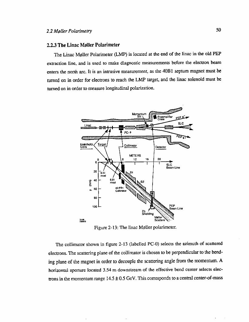
2.2 M@ller Polarimetry 50
2.2.3 The Linac Maller Polarimeter
The Linac Mgller Polarimeter (LMP) is located at the end of the linac in the old PEP
extraction line, and is used to make diagnostic measurements before the electron beam
enters the north arc. It is an intrusive measurement, as the 40Bl septum magnet must he
turned on in order for electrons to reach the LMP target, and the linac solenoid must be turned on in order to measure longitudinal polarization.
loa
Figure 2-13: The linac Moller polarimeter.
The collimator shown in figure 2- 13 (labelled PC-O) selects the azimuth of scattered
electrons. The scattering plane of the collimator is chosen to be perpendicular to the bend-
ing plane of the magnet in order to decouple the scattering angle from the momentum. A horizontal aperture located 3.54 m downstream of the effective bend center selects elec-
trons in the momentum range 14.5 Z!I 0.5 GeV. This corresponds to a central center-of-mass
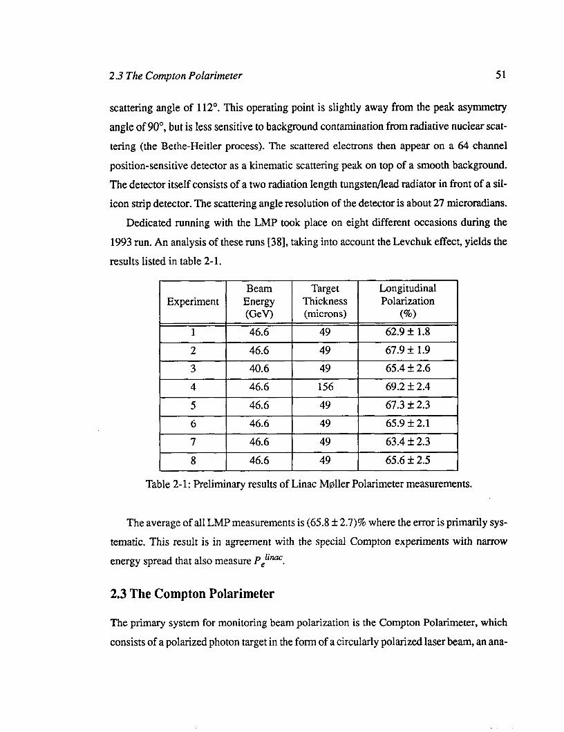
2.3 The Compton Polarimeter 51
scattering angle of 112’. This operating point is slightly away from the peak asymmetry
angle of 90”, but is less sensitive to background contamination from radiative nuclear scat- tering (the Bethe-Heitler process). The scattered electrons then appear on a 64 channel
position-sensitive detector as a kinematic scattering peak on top of a smooth background.
The detector itself consists of a two radiation length tungsten/lead radiator in front of a sil-
icon strip detector. The scattering angle resolution of the detector is about 27 microradians.
Dedicated running with the LMP took place on eight different occasions during the
1993 run. An analysis of these runs [38], taking into account the Levchuk effect, yields the
results listed in table 2- 1.
-‘.‘4... 2 I 46.6
I
7 46.6 8 I 46.6
Target Thickness (microns)
Longitudinal Polarization
(%I I
49 I 62.9 f 1.8 49 I 67.9 f 1.9 49 I 65.4 + 2.6 156 I 69.2 f 2.4
49 I 67.3 AI 2.3 49 65.9 + 2.1 49 63.4 AI 2.3
49 I 65.6 f 2.5
Table 2-l: Preliminary results of Linac Moller Polarimeter measurements.
The average of all LMP measurements is (65.8 f 2.7)% where the error is primarily sys-
tematic. This result is in agreement with the special Compton experiments with narrow
energy spread that also measure PeliMc.
2.3 The Compton Polarimeter
The primary system for monitoring beam polarization is the Compton Polarimeter, which
consists of a polarized photon target in the form of a circularly polarized laser beam, an ana-
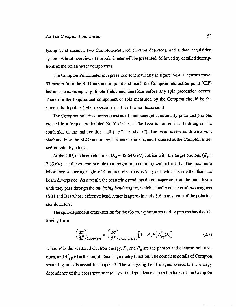
2.3 The Compton Polarimeter 52
lyzing bend magnet, two Compton-scattered electron detectors, and a data acquisition
system. A brief overview of the polarimeter will be presented, followed by detailed descrip- tions of the polarimeter components.
The Compton Polarimeter is represented schematically in figure 2-14. Electrons travel
33 meters from the SLD interaction point and reach the Compton interaction point (CIP)
before encountering any dipole fields and therefore before any spin precession occurs.
Therefore the longitudinal component of spin measured by the Compton should be the
same at both points (refer to section 5.3.3 for further discussion).
The Compton polarized target consists of monoenergetic, circularly polarized photons
created in a frequency-doubled Nd:YAG laser. The laser is housed in a building on the
south side of the main collider hall (the “laser shack”). The beam is steered down a vent shaft and in to the SLC vacuum by a series of mirrors, and focussed at the Compton inter-
action point by a lens. At the UP, the beam electrons (Eb = 45.64 GeV) collide with the target photons (I?,,=
2.33 eV), a collision comparable to a freight train colliding with a fruit-fly. The maximum
laboratory scattering angle of Compton electrons is 9.1 prad, which is smaller than the
beam divergence. As a result, the scattering products do not separate from the main beam
until they pass through the analyzing bend magnet, which actually consists of two magnets
(SB 1 and B 1) whose effective bend center is approximately 3.6 m upstream of the polarim-
eter detectors.
The spin-dependent cross-section for the electron-photon scattering process has the fol-
lowing form
where E is the scattered electron energy, P, and P, are the photon and electron polariza-
tions, and A’,jE) is the longitudinal asymmetry function. The complete details of Compton scattering are discussed in chapter 3. The analyzing bend magnet converts the energy
dependence of this cross section into a spatial dependence across the faces of the Compton
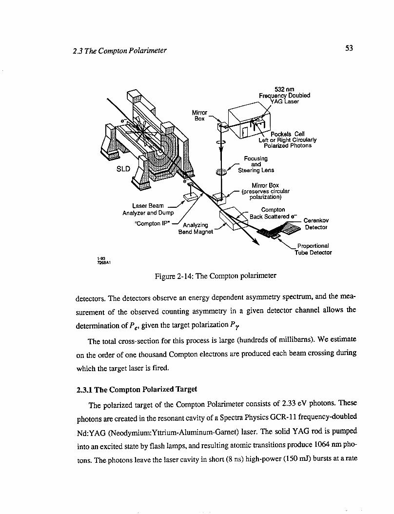
2.3 The Compton Polarimeter 53
532 nm Frequu[~~bled
e/
lady ns
Mirror Box
Cerenkov Detector
l-93 72QQAl
\ \ Proportional Tube Detector
Figure 2-14: The Compton polarimeter
detectors. The detectors observe an energy dependent asymmetry spectrum, and the mea-
surement of the observed counting asymmetry in a given detector channel allows the
determination of P,, given the target polarization P,,
The total cross-section for this process is large (hundreds of millibarns). We estimate
on the order of one thousand Compton electrons are produced each beam crossing during which the target laser is fired.
2.3.1 The Compton Polarized Target
The polarized target of the Compton Polarimeter consists of 2.33 eV photons. These
photons are created in the resonant cavity of a Spectra Physics GCR-11 frequency-doubled
Nd:YAG (Neodymium:Yttrium-Aluminum-Garnet) laser. The solid YAG rod is pumped
into an excited state by flash lamps, and resulting atomic transitions produce 1064 nm pho-
tons. The photons leave the laser cavity in short (8 ns) high-power (150 mJ) bursts at a rate
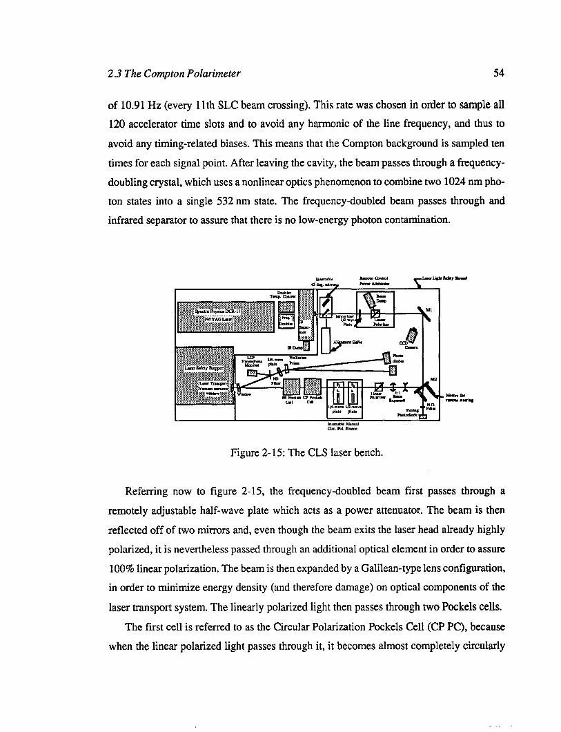
2.3 The Compton Polarimeter 54
of 10.91 Hz (every 1 lth SLC beam crossing). This rate was chosen in order to sample all 120 accelerator time slots and to avoid any harmonic of the line frequency, and thus to
avoid any timing-related biases. This means that the Compton background is sampled ten
times for each signal point. After leaving the cavity, the beam passes through a frequency-
doubling crystal, which uses a nonlinear optics phenomenon to combine two 1024 nm pho-
ton states into a single 532 nm state. The frequency-doubled beam passes through and
infrared separator to assure that there is no low-energy photon contamination.
Figure 2-15: The CLS laser bench.
Referring now to figure 2-15, the frequency-doubled beam first passes through a
remotely adjustable half-wave plate which acts as a power attenuator. The beam is then
reflected off of two mirrors and, even though the beam exits the laser head already highly
polarized, it is nevertheless passed through an additional optical element in order to assure
100% linear polarization. The beam is then expanded by a Galilean-type lens configuration,
in order to minimize energy density (and therefore damage) on optical components of the
laser transport system. The linearly polarized light then passes through two Pockels cells.
The first cell is referred to as the Circular Polarization Pockels Cell (CP PC), because
when the linear polarized light passes through it, it becomes almost completely circularly
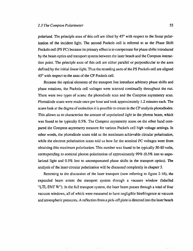
2.3 The Compton Polarimeter 55
polarized. The principle axes of this cell are tilted by 45’ with respect to the linear polar-
ization of the incident light, The second Pockels cell is referred to as the Phase Shift Pockels cell (PS PC) because its primary effect is to compensate for phase shifts introduced
by the beam optics and transport system between the laser bench and the Compton interac- tion point. The principle axes of this cell are either parallel or perpendicular to the axes
defined by the initial linear light. Thus the retarding axes of the PS Pockels cell are aligned
45’ with respect to the axes of the CP Pockels cell. Because the optical elements of the transport line introduce arbitrary phase shifts and
phase rotations, the Pockels cell voltages were scanned continually throughout the run.
There were two types of scans: the photodiode scan and the Compton asymmetry scan. Photodiode scans were made once per hour and took approximately 1.2 minutes each. The
scans look at the degree of extinction it is possible to create in the CP analysis photodiodes.
This allows us to characterize the amount of unpolarized light in the photon beam, which
was found to be typically 0.5%. The Compton asymmetry scans on the other hand com-
pared the Compton asymmetry measure for various Pockels cell high voltage settings. In
other words, the photodiode scans told us the maximum achievable circular polarization, while the electron polarization scans told us how far the nominal PC voltages were from
obtaining this maximum polarization. This number was found to be typically 50-80 volts,
corresponding to nominal photon polarization of approximately 99% (0.5% lost to unpo-
larized light and 0.5% lost to uncompensated phase shifts in the transport optics). The
analysis of the laser circular polarization will be discussed completely in chapter 3. Returning to the discussion of the laser transport (now referring to figure 2-16), the
expanded beam enters the transport system through a vacuum window (labelled
“LTL ENT W”). In the full transport system, the laser beam passes through a total of four
vacuum windows, all of which were measured to have negligible birefi-ingence at vacuum
and atmospheric pressures. A reflection from a pick-off plate is directed into the laser bench
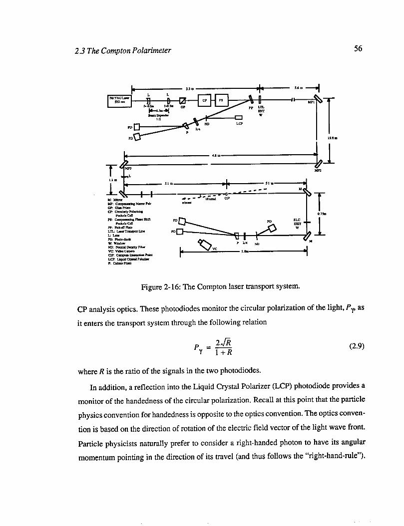
2.3 The Compton Polarimeter 56
- 1.3m I- 5.6m 4
I II
Pn I I 19.6 m
Figure 2-16: The Compton laser transport system.
CP analysis optics. These photodiodes monitor the circular polarization of the light, P, as
it enters the transport system through the following relation
2rR Py = - l+R (2.9)
where R is the ratio of the signals in the two photodiodes.
In addition, a reflection into the Liquid Crystal Polarizer (LCP) photodiode provides a
monitor of the handedness of the circular polarization. Recall at this point that the particle
physics convention for handedness is opposite to the optics convention. The optics conven-
tion is based on the direction of rotation of the electric field vector of the light wave front.
Particle physicists naturally prefer to consider a right-handed photon to have its angular
momentum pointing in the direction of its travel (and thus follows the “right-hand-rule”).
2.3 The Compton Polarimeter 57
In this convention, right-handed photons and right-handed electrons have the same momen- tum characteristic. The particle physics convention is adhered to throughout this document.
Note that there are two reflections which ensures that the handedness going into the LCP
is the same as that entering the transport line.
The transport system itself was at first evacuated, then later run with nitrogen, and
finally filled with 3-5 psi overpressure of helium, in order to minimize optics damage. 1993
running was plagued by optics damage; much more so than 1992. For example, the YAG
rod itself and the Q-switch optics were both replace once during the 1993 run; neither had
any problems during the 1992 runThis was probably due to degradation of the resonant
cavity, which caused “hot-spots” (points of very high energy density) to appear in the laser
beam profile. Such hot spots quickly react with any impurities and escalate damage and
burns on optical surfaces.
An important component of the laser transport system is the mirror-box. The mirror-
box is a construction that allows the beam to be reflected 90’ while maintaining the photon helicity. This is accomplished by having the beam bounce off of two mirrors instead of one
for any change of direction, so that the polarization changes sign after the first bounce, and
then changes sign again after the second bounce. Also, by using identical (i.e. manufactured
at the same time) dielectric mirrors, any phase-delay introduced by surface effects in the
first mirror is exactly compensated for and removed by the second mirror.
After the CLS laser beam passes through three such mirror-boxes, it enters the lens box,
where a remotely moveable 5 m focal length lens focuses and steers the beam for collision
with the electrons. After one more mirror-box reflection, the photons enter the SLC vacuum
through a window at an angle of 10 milliradians with respect to the electron beam. At the
CIP, the RMS electron beam size is 350 microns, and the photon beam size is 500 microns.
After collision, the laser beam exits the SLC vacuum, and is reflected by an uncompensated
mirror into the laser analysis box. The analysis box contains CP analysis optics in the same
configuration as on the laser bench, see figure 2-17. The final uncompensated reflection
introduces a large phase shift between the CIP and the analysis box, which is why the anal-
ysis box data cannot be taken as a direct measurement of the laser polarization at the CIP.

2.3 The Compton Polarimeter 58
Figure 2-17: The CLS analysis box optics
2.3.2 The Cherenkov Detector
The ideal polarimeter detector requires good position resolution and background sup-
pression. The position spectrum of the scattered electrons must be carefully measured in
order to extract the beam polarization. With these requirements in mind, a simple Cheren-
kov design was selected. The Cherenkov detector consists of nine 1 cm x 1 cm polished
aluminum channels, filled with static sys-trans-2-butene gas at atmospheric pressure, end-
ing at nine Hamamatsu R1398 photomultiplier tubes with custom bases designed at the
Lawrence Berkeley Laboratory. The phototube base is also an important component of the overall detector design. In
order to fully calibrate the detector, it is necessary to determine the linearity characteristics
of the phototubes. This is done by monitoring the asymmetry in one channel with a fixed signal height, and comparing this to the asymmetry measure in a channel whose signal
height is varied. As the phototube saturates, the larger (parallel electron-photon spins) sig- nal is measured lower than its true value, and the asymmetry in this channel decreases
relative to the control channel. The problem is, that in order to change the signal height in
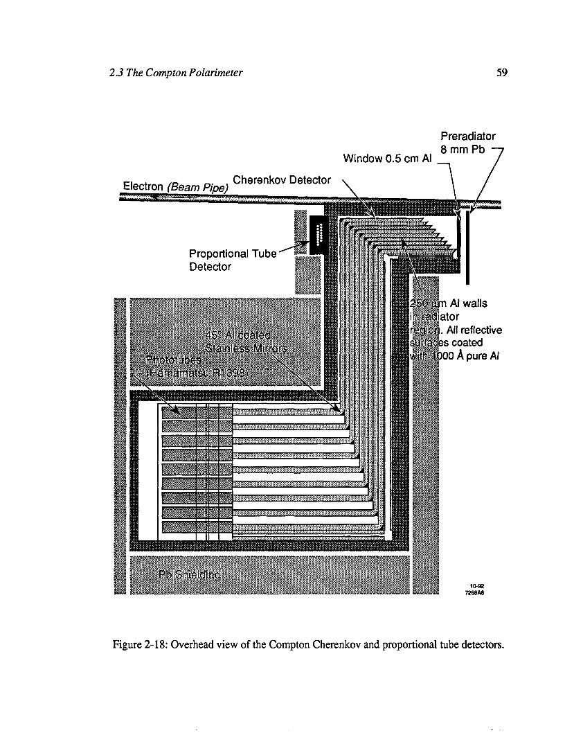
e 8 1 \

2.3 The Compton Polarimeter 60
a channel, one must change the gain of the phototube, which in turns changes the space- charge characteristics of the amplifying stages, which in turn changes the saturation char-
acteristic. The purpose of the LBL phototube base design is to allow the voltage on the
front-end of the dynode chain to be varied, thus changing the gain of the phototube, and yet
keep the back-end voltages fixed, thus maintaining a constant space-charge and thereby a constant saturation characteristic. Without this important characteristic, any measurement
of the phototube linearity involving gain adjustments would be suspect. This base design is
discussed in greater detail in Reference [39]. When Compton-scattered electrons leave the SLC vacuum through a thin window, they
pass through a lead radiator. The high energy shower products enter the Cherenkov chan-
nels through a 0.5 cm aluminum window, where they travel faster than the speed of light in
that medium and thus emit Cherenkov light (the Cherenkov threshold of the gas is approx-
imately 10 MeV). This light travels down the aluminum channels, is reflected off of
polished, aluminum-coated stainless steel mirrors, and is detected in the photomultiplier
tubes. The amount of Cherenkov light produced is proportional to the number of Compton
scattered electrons.
The Cherenkov detector housing is surrounded by lead in order to shield the phototubes
from any backgrounds. The detector assembly rests on a thick aluminum plate, which
moves perpendicular to the beam-line on a set of precision bearings. The plate (henceforth
referred to as the table) is driven by a stepping motor and its position is monitored by a lin-
ear potentiometer. The table is nominally at the inner-most position (as close to the main
beam as possible), resting against a physical stop. The potentiometer reference voltage and
position voltage are read by a SAM (smart analog module) at the end of every polarimeter
run, so that the detector has no systematic uncertainty associated with the table being out
of position.
The table movement is a useful tool for the determination of the absolute location of the
detector relative to the main beam, which is in turn an essential input for the calibration of
the detector analyzing powers. Such a determination is called an edge scan. Edge scans rely
on the fact that the Compton cross-section has a sharp kinematic endpoint, corresponding
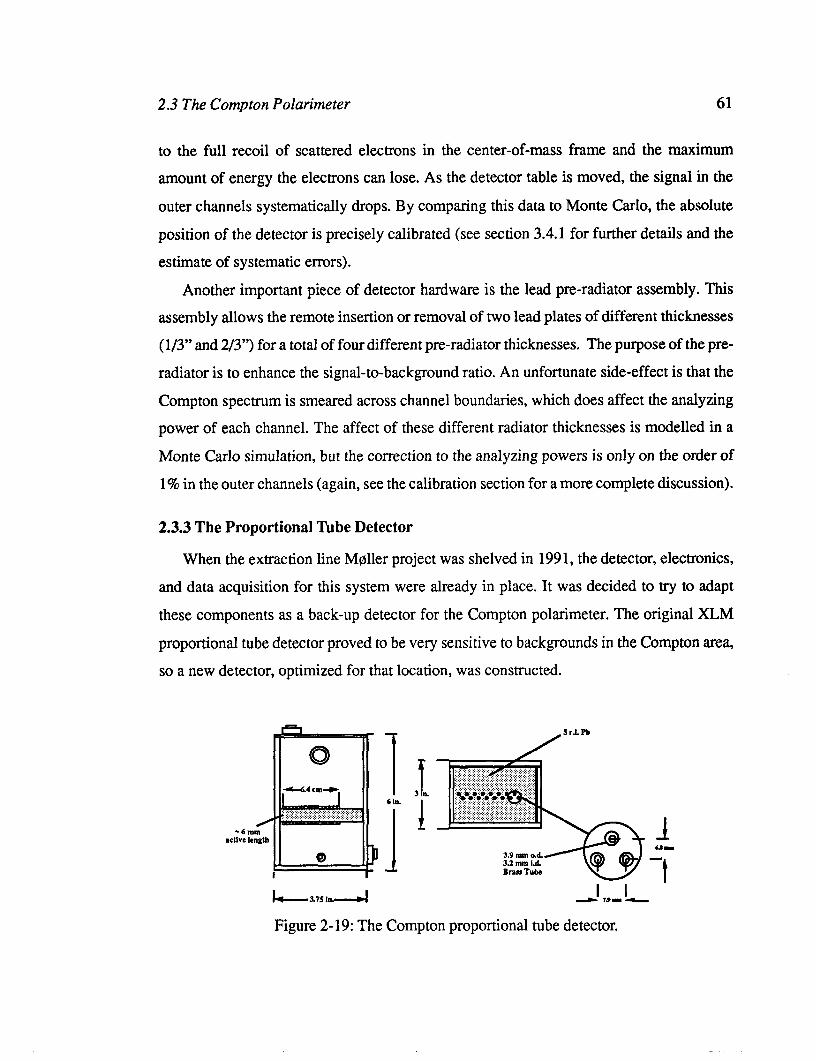
2.3 The Compton Polarimeter 61
to the full recoil of scattered electrons in the center-of-mass frame and the maximum
amount of energy the electrons can lose. As the detector table is moved, the signal in the
outer channels systematically drops. By comparing this data to Monte Carlo, the absolute
position of the detector is precisely calibrated (see section 3.4.1 for further details and the
estimate of systematic errors).
Another important piece of detector hardware is the lead pre-radiator assembly. This assembly allows the remote insertion or removal of two lead plates of different thicknesses
(l/3” and 2/3”) for a total of four different pre-radiator thicknesses. The purpose of the pre-
radiator is to enhance the signal-to-background ratio. An unfortunate side-effect is that the
Compton spectrum is smeared across channel boundaries, which does affect the analyzing
power of each channel. The affect of these different radiator thicknesses is modelled in a
Monte Carlo simulation, but the correction to the analyzing powers is only on the order of
1% in the outer channels (again, see the calibration section for a more complete discussion).
2.3.3 The Proportional tibe Detector
When the extraction line Moller project was shelved in 1991, the detector, electronics,
and data acquisition for this system were already in place. It was decided to try to adapt
these components as a back-up detector for the Compton polarimeter. The original XLM
proportional tube detector proved to be very sensitive to backgrounds in the Compton area,
so a new detector, optimized for that location, was constructed.
6 la. 1
Figure 2-19: The Compton proportional tube detector.
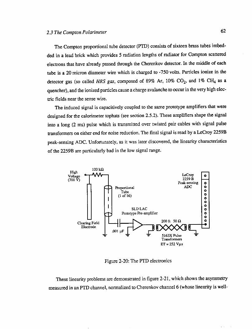
2.3 The Compton Polarimeter 62
The Compton proportional tube detector (PTD) consists of sixteen brass tubes imbed-
ded in a lead brick which provides 5 radiation lengths of radiator for Compton scattered
electrons that have already passed through the Cherenkov detector. In the middle of each
tube is a 20 micron diameter wire which is charged to -750 volts. Particles ionize in the
detector gas (so called HRS gas, composed of 89% Ar, 10% COZ, and 1% CH4 as a
quencher), and the ionized particles cause a charge avalanche to occur in the very high elec- tric fields near the sense wire.
The induced signal is capacitively coupled to the same prototype amplifiers that were designed for the calorimeter tophats (see section 2.5.2). These amplifiers shape the signal
into a long (2 ms) pulse which is transmitted over twisted pair cables with signal pulse transformers on either end for noise reduction. The final signal is read by a LeCroy 2259B
peak-sensing ADC. Unfortunately, as it was later discovered, the linearity characteristics
of the 2259B are particularly bad in the low signal range.
C > Proportional Tube
LeCroy 2259 B
Peak-sensing ADC
I (1 of 16)
I SLD LAC Prototype Pre-amplifier
Clearing Field Electrode
0
0 0 0 0 0
1 0 0 0 0 0 0
Transformers ET = 252 Vps
Figure 2-20: The PTD electronics
These linearity problems are demonstrated in figure 2-21, which shows the asymmetry
measured in an PTD channel, normalized to Cherenkov channel 6 (whose linearity is well-

2.3 The Compton Polarimeter 63
understood, see section 3.3.2) as a function of the PTD pulse height. So far, the PTD system
has not provided a precise independent measurement of the beam polarization, as hoped.
Figure 2-21: The PTD linearity from 1993 data.
2.3.4 Data Acquisition
The polarimeter data acquisition, represented in figure 2-22, consists of three stages:
The CAMAC crates, the M2ELN microvax, and the SLDACQ VAX. One CAMAC crate
is located in the mezzanine above the SLD control room; two others are located in the laser
shack. The microvax is also located in the SLD mezzanine, directly above the first
CAMAC crate. The interface between the microVax and the CAMAC crates is a Kinetic
Systems Serial Highway driver. Ribbon cables connect M2ELN to the first CAMAC crate.
A fiber optic line connects crate one to the laser shack crates 2 and 3. M2ELN is in turn
linked to the SLDACQ VAX cluster via an ethernet connection.

2.3 The Compton Polarimeter 64
SLD VAX Cluster
SLD Data Tape
Data Logger
- M2ELN pvax & ’ E POLSERVER d 2 : POLXP 4 - Ethernet
KS 2160 connection SLDACQ SLD User Terminal
I
CAMAC b CAMAC CAMAC Crate 1 4 Crate 2 Crate 3
fiber optic line \
Figure 2-22: Schematic representation of the Compton polarimeter data acquisition
Every beam crossing, an SLC base rate trigger (TRBR) triggers ADC gates on modules
in the three CAMAC crates. These triggers are farmed out through delay generators in order
to properly gate each module. The very last gate to be initiated triggers a CAMAC LAM
(“Look-At-Me”) which causes the M2ELN microvax to read all of the modules. Fifty-three
words (106 bytes) of Polarimeter data are collected every beam crossing. This raw data is
stored in a local ring buffer. Once 150 beam crossings have been accumulated in the ring
buffer, M2ELN sends the entire buffer to the SLD VAX via ethernet, where it is handled
by the POLSERVER process. POLSERVER logs data in two modes simultaneously. In the first mode, the raw data
packet of 150 beam crossings is written to SLD data tape in a sparsified manner, with only
one background (laser off) state per signal (laser on) state, instead of the available ten to
one ratio, in order to minimize tape input/output. Background pulses are chosen two beam
crossings before the signal crossing, in order to measure background on the same (even or
odd) time slot, with no signal-related bias. During 1993, raw polarimeter data accounted for
ten to twenty percent of data written to SLD tape.
2.3 The Compton Polarimeter 65
In the second mode, histograms of sums and sums-squared are accumulated by the
POLSERVER process. The PLS helicity state is decoded from the crate 1 register and can
have three possible values: left-handed, right-handed, and error. During the 1993 run, the
Polarimeter relied on the Mach line transmission of the PLS helicity bits. The CLS helicity
state is decoded from the crate 3 data register and can have four possible values: left-
handed, right-handed, unpolarized, and off. Machine data (toroids and beamstrahlung) are
binned in histograms based on the PLS helicity state. Laser data (photodiodes) are binned
based on the CLS helicity state. Detector data (Cherenkov and PTD channels) are binned
based on the CLS and PLS helicity states.
If any of the following conditions are true for a given beam crossing, the data from that
beam crossing is not summed into any histogram: North electron toroid less than 100 ADC
counts (eliminates missing electron pulses), north positron toroid less than 100 ADC counts (eliminates missing positron pulses), and Cherenkov channel 9 signal greater than 200
ADC counts (eliminates very noisy pulses in the Cherenkov detector). The veto conditions are selected by operators through the POLSERVER process. Oper-
ators interface with the POLSERVER process through SCPs (SLAC Control Panels).
Although the default running conditions automatically activate all vetoes, it is possible for
data to be accumulated with one or many of the vetoes inactive. Polarimeter runs for which
the normal vetoes were inactive are removed during the analysis phase (see section 3.7).
After a designated number of accumulated beam crossings (typically 20,000),
POLSERVER requests a read of the crate 3 SAM, which monitors the table position and
detector voltages, and a read of an IDIM which monitors the lead pre-radiator status. Then
the summary buffers and SAM data are also written to SLD data tape. The main polarimeter
analysis makes use of these summary data banks.
In addition to the data acquisition described above, which is driven by beam crossing
triggers, there is data taken on an hourly basis, initiated automatically. Each hour, the read
and write lines of each CAMAC crate are tested with SLD crate verifiers. Additionally, the
Pockels cell voltages are scanned about the nominal points, and the resulting photodiode
readings are written to SLD data tape.

2.4 The Energy Spectrometer 66
There is one further complication in normal data acquisition. Since April 27, 1993, the so-called AUTOPOCKSCAN running mode was made the default running condition. In
this mode, the CLS Pockels cell voltages are set away from nominal for two out of three
polarimeter runs. In this manner, we effectively scan the Compton asymmetry as a function
of Pockels cell voltage. These scans are fit off-line for the laser polarization as a function
of the voltage settings (refer to section 3.5 for full details). The implementation of this scan-
ning mode has enabled us to reduce the systematic error on laser polarization to below 1%.
In theory, all runs could be used, if properly corrected for the voltage offsets. However, the
error associated with the correction is a steep function of the offset itself; therefore electron
polarizations for the A,Q analysis are calculated only using runs in which both the CP and
PS Pockels cells are at their nominal voltage settings (we will hereby refer to such runs as
nominal runs).
2.4 The Energy Spectrometer
The last hardware element encountered by electrons before they enter the beam dump is an
energy spectrometer [40]. The layout of this spectrometer is shown in figure 2-23. The
positron energy is measured by an identical spectrometer in the positron extraction line.
Spectrometer Quadrupole Magnet
hrotron Radiation
2-90
Figure 2-23: The electron extraction line energy spectrometer.
In each spectrometer, the beam passes through three dipole magnets, of which the sec-
ond is a precision analysis magnet. The first and third magnets bend the beam perpendicular
2.5 The SLD Detector 67
to the bend plane of the analysis magnet, and cause the beam to emit to parallel stripes of
synchrotron radiation. A detector known as the WISRD (Wire Imaging Synchrotron Radi-
ation Detector) is located approximately 15 m downstream of the analysis magnet. The WISRD consists of two screens of 96 copper wires each (the synchrotron stripes are
detected via Compton scattering of electrons off of the wires) which measure the distance
between the two synchrotron stripes. This distance (approximately 26 cm) determines the
deflection angle of the beam, 6, through the analysis magnet which is in turn related to the
beam energy, Eb through
(2.10)
where B is the magnetic field of the analysis magnet and dl lies along the beam path.
Because Am is a function of center-of-mass energy, a precise measurement of this
quantity is essential to the experiment. The spectrometer is capable of measuring an instan-
taneous energy of a single beam to within 22 MeV. Most of this error is due to electronic
noise, which averages out over many pulses. Therefore the average energy of a single beam
is measure to within 12 MeV [41]. During the 1993 run, the energy spectrometer measured
the average center-of-mass energy at 91.26 f 0.02 GeV, and the average electron beam
energy at 45.64 + 0.01 GeV.
2.5 The SLD Detector
The SLC Large Detector, or SLD, was proposed in 1984 [42] and was intended to be the
main detector for SLC 2 physics. The detector was completed in 1991 and replaced the
Mark II detector at the main interaction point. A cutaway view of the detector is shown in
figure 2-24. The design incorporates all the elements of modem detectors, including a pre-
cision silicon vertex detector and a Cherenkov ring imaging detector.
The ALR measurement is not dependent on an analysis of the Z decay final states, and
need not make use of the tracking and particle identification systems. It has been suggested
that, for the purpose of this measurement, the entire detector could be replaced by a few
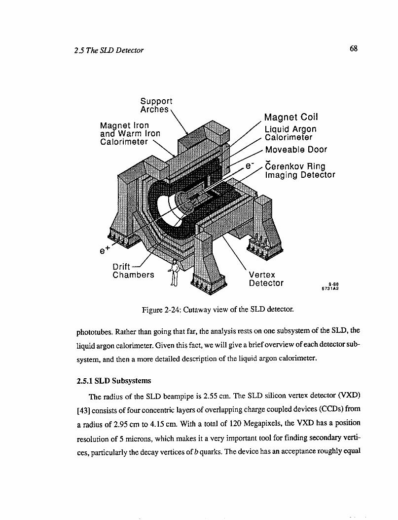
2.5 The SLD Detector 68
support Arches
Ma net Iron an 8 Warm Iron Calorimeter \
Moveable Door
ing Detector
Drift J Chambers
b Detector 9-88 C-J.a.1”
Figure 2-24: Cutaway view of the SLD detector.
phototubes. Rather than going that far, the analysis rests on one subsystem of the SLD, the
liquid argon calorimeter. Given this fact, we will give a brief overview of each detector sub-
system, and then a more detailed description of the liquid argon calorimeter.
2.5.1 SLD Subsystems
The radius of the SLD beampipe is 2.55 cm. The SLD silicon vertex detector (VXD)
[43] consists of four concentric layers of overlapping charge coupled devices (CCDs) from
a radius of 2.95 cm to 4.15 cm. With a total of 120 Megapixels, the VXD has a position
resolution of 5 microns, which makes it a very important tool for finding secondary verti- ces, particularly the decay vertices of b quarks. The device has an acceptance roughly equal
2.5 The SLB Detector 69
to that of the central drift chamber, and data from these two systems can be combined in order to improve the overall momentum measurement.
The luminosity monitor (LUM) [44] is encountered by particles with a very small scat-
tering angle (35 mrad < 8 < 68 mrad). This system has a small angle, high precision
electromagnetic calorimeter at both the north and south ends of the detector. Each calorim-
eter consists of 23 tungsten radiator plates approximately one radiation length thick,
instrumented with silicon detectors in the plate gaps. The e+e- scattering process is domi-
nated by t-channel photon exchange at small angles, and the LUM system detects these
electrons at a rate which is approximately two times the Z production rate, with an energy
resolution of approximately 3.0% for a 50 GeV electron.
A particle traveling with slightly larger scattering angle (> 700 mrad) encounters the
central drift chamber (CDC). The drift chamber is a cylindrical array of sense wires,
extending from a radius of 0.2 m to 1.0 m. In the presence of the 0.6 Tesla solenoidal mag-
netic field provided by the SLD magnet, the CDC provides momentum and position
measurements of charged particles. The measured momentum resolution for the CDC was
approximately (0.0095)2/p2 + (0.0049)2 with a local spatial resolution of 100 microns. In
addition to the CDC, the SLD is also instrumented with four endcap drift chambers (EDCs)
which were to complement the CDC measurement in the forward region (]cos0] > 0.71).
The next radial system is the Cherenkov Ring Imaging Device (GRID) [45], which was
designed to provide particle identification over a large range of momenta. The GRID
employs a hybrid system of gas (CsF12) and liquid (C6F14) Cherenkov radiators and
TMAE-based TPC detectors in order to achieve the widest possible momentum acceptance. The CRID also has separate central and endcap subsystems, neither of which is yet used in
physics analysis.
The SLD calorimetric system is a hybrid of lead-liquid argon and iron-gas sampling
calorimeters. The inner system, the Liquid Argon Calorimeter (LAC), is described in the
next section. The massive outer structure of the Warm Iron Calorimeter (WIG) [46] acts as
a muon identifier and a magnetic flux return, as well as a calorimeter, and is also subdivided
into central and endcap subsystems. The central system consists of eight chambers arranged
2.5 The SW Detector 70
octagonally, each chamber consisting of seven alternating steel/air-gap layers. The air gaps
are instrumented with streamer tubes. The WIG system provides a o/E measurement of 8O%/fi, as well as some tracking information.
2.5.2 The Liquid Argon Calorimeter
Liquid argon sampling calorimeters have several desirable properties that lend them-
selves to Z physics. They allow large solid angle coverage and have excellent energy
resolution and uniformity of response. They may have arbitrarily fine segmentation and they offer good radiation resistance, allowing for operation close to the beamline within the
magnetic fields.
The location of the SLD liquid argon sampling calorimeter with respect to the rest of
the detector is most clearly shown in figure 2-25. The LAC is composed of a cylindrical
barrel calorimeter and two endcap calorimeters [47]. The barrel section covers the region of 8 2 33” (Icosel I 0.84) and is composed of 288 modules mounted in a cylindrical cry-
ostat. In the radial direction, two separate types of modules are mounted on top of each
other, the electromagnetic (EM) modules and the hadronic (HAD) modules. The endcap
calorimeters cover the region 8’ < 8 < 35” (0.82 > 1~0~01 > 0.99), and are composed of 16
wedge-shaped modules, each module also containing an EM and HAD section.
Endcap modules differ from barrel modules in design and construction, but are func-
tionally identical, so we will describe the barrel-type module only, which is pictured in
figure 2-26. The modules are constructed as parallel plate ionization chambers, with alter-
nate planes of lead sheets and segmented lead tiles serving as the absorber, with liquid
argon filling the gaps between the planes. The tile geometry forms projective towers, rep-
resented by dashed lines in figure 2-25, which point toward the interaction point. The LAC is longitudinally divided into four compartments, two electromagnetic fol-
lowed by two hadronic. The first EM compartment contains 8 cells for a total of 6 radiation
lengths (6 X0). The second EM compartment contains 20 cells for a total of 15 radiation
lengths. This total EM thickness contains 98% of the energy from a 50 GeV electron. The
EM sections are followed by two HAD compartments of 13 cells and 1 absorption length

2.5 The SLB Detector 71
Maanet Coil
Endcap WIG
Detector Monitor Beamline 10-92
7282A2
Figure 2-25: Quadrant view of the SLD detector.
(1 ho) each. The total thickness of the EM and HAD sections is 2.8 ho, which contains 80-
90% of the energy from a hadronic shower. The LAC is divided transversely into 32,448
towers in the barrel section, 8,640 towers in the endcap, and covers the full solid-angle up
to lcosej 50.98.
The first step LAC data acquisition chain is a set of electronics called tophats, which
are mounted on the detector itself and provide amplification and digitization of the tower
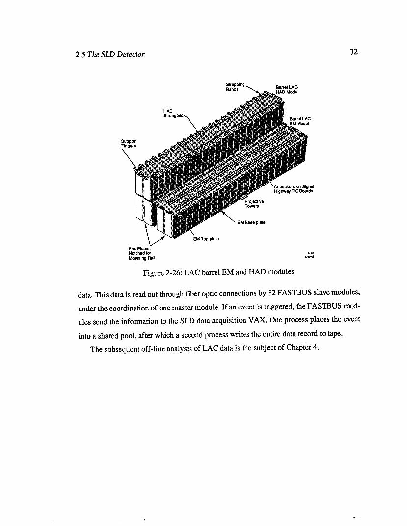
2.5 The SLB Detector 72
End Plates; Notched for Mounting Rail
Figure 2-26: LAC barrel EM and HAD modules
data. This data is read out through fiber optic connections by 32 FASTBUS slave modules,
under the coordination of one master module. If an event is triggered, the FASTBUS mod- ules send the information to the SLD data acquisition VAX. One process places the event
into a shared pool, after which a second process writes the entire data record to tape.
The subsequent off-line analysis of LAC data is the subject of Chapter 4.

Chapter 3
Compton Polarimetry
Electron polarization is the most unique and important aspect of the Am experiment and
also contributes the largest systematic uncertainty to the experiment. The Compton Pola-
rimeter provides a precise monitor of the longitudinal beam polarization through the well- understood QED process of Compton scattering. This chapter will address the details of
Compton scattering kinematics, polarization extraction (polarimetry), polarimeter data
selection, and systematic errors.
3.1 Compton Scattering Kinematics
The elastic scattering of an electron and photon, known as Compton scattering, is
described, to lowest order in QED, by an s-channel and u-channel electron exchange, as
illustrated in figure 3-l.
As was previously described, the energy of the photon in the laboratory frame is
2.33 eV, while the energy of the electron is 45.6 GeV. This makes working in the labora-
tory frame somewhat cumbersome. However, the analyzing magnets and polarimeter
detectors live in the laboratory frame, so we require cross sections in this frame. We will
start with the known cross section in the rest frame of the electron and then outline the
transformation of variables from the rest frame to the laboratory frame.
73
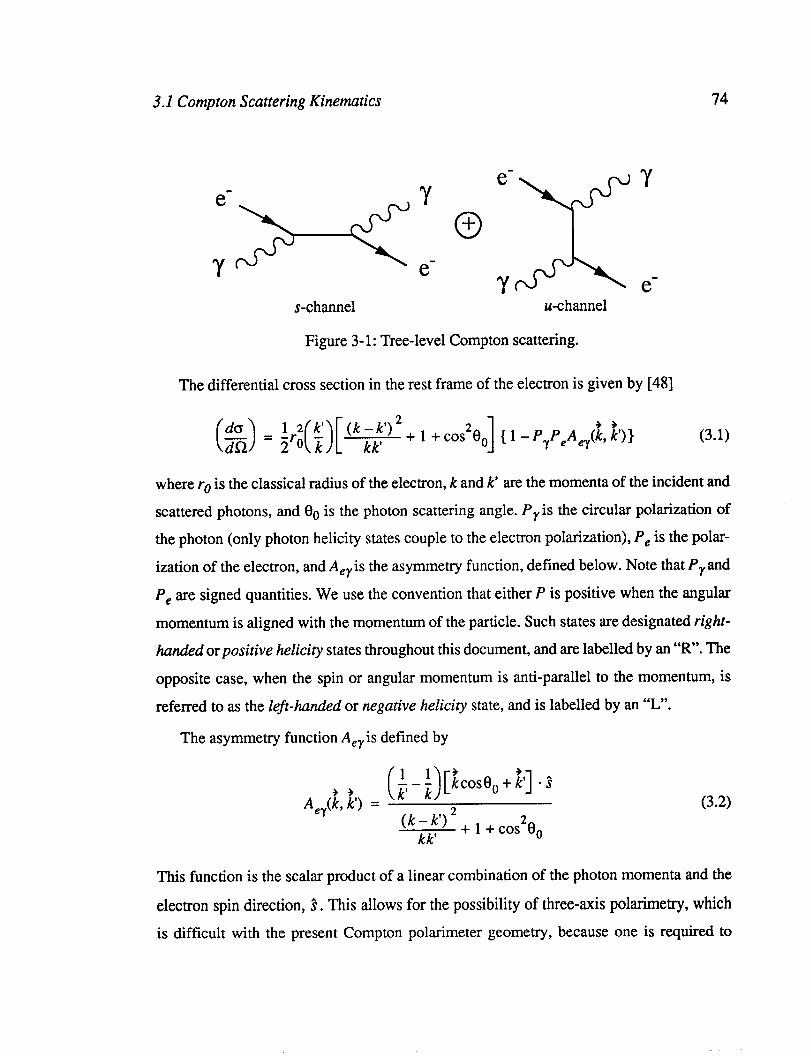
3.1 Compton Scattering Kinematics 74
s-channel u-channel
Figure 3- 1: Tree-level Compton scattering.
The differential cross section in the rest frame of the electron is given by [48]
+ 1 + cos28u ] { 1 - P,PcA$, ;I)} (3.1)
where rO is the classical radius of the electron, k and k’ are the momenta of the incident and
scattered photons, and 00 is the photon scattering angle. P,is the circular polarization of
the photon (only photon helicity states couple to the electron polarization), P, is the polar-
ization of the electron, and A,,is the asymmetry function, defined below. Note that P,and
P, are signed quantities. We use the convention that either P is positive when the angular
momentum is aligned with the momentum of the particle. Such states are designated right-
handed orpositive helicity states throughout this document, and are labelled by an “R”. The
opposite case, when the spin or angular momentum is anti-parallel to the momentum, is
referred to as the left-handed or negative helicity state, and is labelled by an ‘I”.
The asymmetry function A,,is defined by
(3.2)
This function is the scalar product of a linear combination of the photon momenta and the
electron spin direction, ?. This allows for the possibility of three-axis polarimetry, which is difficult with the present Compton polarimeter geometry, because one is required to
3.1 Compton Scattering Kinematics 75
detect the scattered photons, which diverge only minimally from the beamline. Neverthe-
less, research and development for a three-axis Compton polarimeter at SLAC is already
underway. The 1993 Compton polarimeter, which detects only scattered electrons, is only
useful for longitudinal polarization measurements, a point which is discussed in section
(3.2.2) below.
3.1.1 Laboratory Frame Scattering Kinematics
We define E and K to be the incident energies of the electron and photon, and E’ and K’ to be the scattered energies of the electron and photon. We now introduce the Compton
scattering y parameter which is the ratio of the minimum scattered electron energy to the
incident electron energy:
(3.3)
E min = Ey
The electron has it’s minimum energy in the case of complete backscattering in the center- of-mass frame. The emission angle of the scattered photon is then related to the scattered
photon energy through the following expression
K’ = K’,,[l +y(~)3-1_g’max.x (3.4)
wherein the kinematic variable x is defined. The values of x range from zero (no scattering)
to one (full backward scattering, the kinematic endpoint).
The transformation between the electron rest frame and the laboratory frame variables
is defined through the following equations:
K 1 - coseu X
= - = 2y+ (1 +y) (1 -cose(J K’ max
(3.5)

3.1 Compton Scattering Kinematics 76
Applying this transformation to equations (3.1) and (3.2) yield the expression for the cross section in the laboratory frame, in terms of the laboratory variables x and y:
{ 1 -P, [P:A&) + P:cos@(&J] 1 (3.6)
where $ is the is the azimuthal angle of the photon with respect to the transverse polariza-
tion component of the electron, and the superscripts z and t refer to the longitudinal and
transverse polarization components, respectively. The unpolarized cross section is given by
(3.7)
and the longitudinal and transverse asymmetries are defined by
Ah = riy[l -x(1 +y)] l- 1
wxu-Y>12 (3.8)
Figure 3-2 shows these asymmetries and the cross section plotted as a function of the kine- matic variable x.
3.1.2 Radiative Corrections
The first-order radiative corrections to polarized Compton scattering have been calcu-
lated [49]. The effects are less than 0.3% on the unpolarized cross section and less than
0.1% on the asymmetry of the outer channels. It is conceivable that these corrections will
become important in a future analysis that would use the full Compton spectrum and
attempt to measure the polarization to within 0.5%. However, radiative corrections are
ignored in the 1993 analysis.

3.2 Extracting the Beam Polarization from Compton Scattering 77
6-93
600 600 I I I I I I I I I I I I I I I I I I 1.2 1.2 4 4 * * /- /-
--were- --were- 200 200 - - 0.4:
E
I I I I I I I I I I I I ,Az I ,Az I I I -0.2 -0.2 0 0 0.2 0.2 0.4 0.4 0.6 0.6 0.8 0.8 1.0 1.0
x=K'/K',, x=K'/K',, 6004A14 6004A14
Figure 3-2: The Compton cross section and asymmetries. Figure 3-2: The Compton cross section and asymmetries.
3.2 Extracting the Beam Polarization from Compton Scattering
The remainder of this chapter deals with the specifics of Compton polarimeter analysis,
including the bend magnets, the target, and the detectors. The first detailed account of Cher-
enkov detector analysis appears in Reference [SO]. An updated account for the 1993 run
follows, much of which is derived from the content of Reference [Sl].
We have shown that the QED process of Compton scattering has an intrinsic asymme-
try and that the cross section can be separated into polarized and unpolarized parts. In this section we discuss how the analyzing bend magnet of the polarimeter translates an asym-
metry as a function of energy into an asymmetry as a function of distance. We then describe
how this new function is measured as an experimental asymmetry in a detector.

3.2 Extracting the Beam Polarization from Compton Scattering 78
3.2.1 The Analyzing Bend Magnet
In the laboratory frame, Compton electrons are scattered very much in the forward
direction. The maximum electron scattering angle of 9.1 radians is considerably less than
the beam divergence. Thus the Compton scattered electrons travel colinearly with the main
electron beam until they pass through the first dipole bending magnets (B31 and B32, the
so-called soft and hard bending magnets), the combination of which is referred to as the
analyzing bend magnet of the polarimeter. These magnets provide a transverse momentum kick to the electrons and thereby couple the scattered electron energy E, with a spatial dis-
tance s, measured perpendicularly from the infinite momentum line, through the following
relation
BD BD S Z-E
E E,[~-~U-Y)I (3.10)
where B is the effective bend strength of the two magnets, D is the distance from the effec-
tive bend center of the magnets along the neutral beam line from which s is measured, Eb
is the beam energy, and x and y are the kinematic parameters defined in section 3.1.1. In the
case of the polarimeter, s is measured at the entrance of the Cherenkov detector channels.
For the nominal beam and target energies, y = 0.3804.
I I
effective I
Figure 3-3: The analyzing bend magnet of the Compton polarimeter.
3.2 Extracting the Beam Polarization from Compton Scattering 79
The geometry of the analyzing bend magnet is clarified in figure 3-3 (the angles and
distances are not drawn to scale). The design bend angle of magnet SBl is 1.0 mrad. The
design bend angle of magnet Bl is 17.27 n-n-ad. The distance d between the bend centers of
the magnets is 385.7 cm. Thus the effective bend center occurs at a distance 1 = 22.3 cm
from the center of B 1. The effective bend angle of the combined analyzing magnet is
18.27 mrad (833.2 MeV/c). The distance from the effective bend center to the face of the detector, D, has been measured to be 355.8 cm. Therefore s1 (the distance from the neutral
beamline to the main beamline) is (BD)/Eb = 6.50 cm, and s2 (the distance from the neutral
beamline to the Compton kinematic endpoint) is (BD)/(Eby) = 17.08 cm.
The combination of these numbers with equation (3.10) gives us the transformation
Jacobian necessary to go from the cross section as a function of the energy variable x to the
cross section as a function of the space variable s:
(3.11)
where the differential cross section with respect to x is fully defined by equations (3.6)
through (3.9).
3.2.2 The Experimental Asymmetry
Because the laboratory scattering angles are so small in the Compton polarimeter, all
scattered electrons are swept into the same energy-space correlation by the bending mag-
nets, regardless of their azimuth. Thus the detector effectively integrates over the azimuthal
distribution and eliminates the transverse asymmetry term in the cross section. We simplify
the expression for the cross section even further by absorbing the unpolarized cross section
(including dxlds) into the function U(s), and the remaining polarization-dependent part into
the function A(s), writing
U(s) [ 1 + Pf’:A(s)] (3.12)
where s is the transverse spatial coordinate at the detector.

3.2 Extracting the Beam Polarization from Compton Scattering 80
It follows from (3.12) that the observed or measured asymmetry in a given channel i,
A;, is directly related to the product of the electron and photon polarizations
A; = NF + NY-NY - N$ Ny+Ny+Ny+N$
= PYPfai (3.13)
XY where Ni = O;‘-B;
The number of observed Compton electrons in channel i, Ni”, is equal to the average num-
ber of counts observed in the channel in the given helicity combination XY, Oixy, minus
the background observed in that channel when the laser is off, Bix. Note that the back-
ground term does depend on the electron helicity state; this takes into account any
background-related asymmetry. The two superscripts refer to the helicity state of the elec-
trons and photons respectively. The LR and RL states corresponds to a J~D spin combination, when the electron and photon angular momenta are parallel. The LL and RR
states represents the J~D combination, where the photon and electron angular momenta are
anti-parallel. The J3/2 case is the larger cross section in Compton scattering [52]. Py is the
circular polarization of the laser, P,’ is the electron polarization measured at the Compton
interaction point, and ai is the analyzing power of channel i.
The analyzing power is defined by the following expression
a i
= /‘(s) A(s) Pi(S>dS
I u(S) Pi(S)dS (3.14)
where p is response function (acceptance as a function of s) for channel i. The analyzing
power of a channel is the average of the Compton asymmetry, weighted by the unpolarized
cross section (which is relatively flat across the detector acceptance) and the detector
response function, p, for that channel. If we recast equation (3.13), we see that the measure-
ment of the beam polarization, P,‘, rests on the measurement of the experimental

3.3 Measuring the Experimental Asymmetry 81
asymmetry, the determination of the analyzing powers, and the measurement of the laser
polarization.
A; pf = -
a.P i Y
(3.15)
The quantities on the right hand side of equation (3.15) are the topics of the following
sections.
3.3 Measuring the Experimental Asymmetry
This section describes four potential problems facing the experimental asymmetry mea-
surement: contamination by other asymmetries such as photon and/or electron current asymmetries, the effects of non-linear detector response, the effects of signal-correlated
background noise, and the effects of saturated detector pulses.
3.3.1 Compton Asymmetries
Measurement of the experimental asymmetry rests on a proper accounting of the four
Compton asymmetries that affect the observed asymmetry: the left-right asymmetries in the
electron and photon currents, and the left-right polarization asymmetries of the electron and
photon beams. We define these asymmetries (the A quantities) through the following
relations:
p: = (1 +AP,)P;
P; = (1 +APy,P;
t = ( 1 + AI,) Ze
I; = (1 +A$)$,
p: = (1 -AP,)P;
P; = (1 -AP,) P;
I,” = (1 -AZ&
Z; = (1-AI&
It can be shown that the measured asymmetry A; defined in the previous section is
independent of all the A quantities defined above, to first order in those asymmetries.
Therefore the measured asymmetry A; is the correct quantity to use in the Am analysis,
as described in section 1.5.1 However, we are also interested in making corrections to the

3.3 Measuring the Experimental Asymmetry 82
assumption that the polarization asymmetry is zero, in which case it is necessary to use more polarimeter information.
It can also be shown that the “asymmetry asymmetries” in a given channel i are related
to the A quantities in the following manner:
+-NY NfR-N; - = Nr+Ny Ny+Ny
2 [AI, + AfAPy - A;A; (AI, + Ape)] (3.16)
NF-NY I$“-N; - = N;+N; Ny+N;
2 [AI, + A;APe - A;Af (AI, + AP,)] (3.17)
Each channel makes an independent measurement of the quantities defined in equations
(3.16) and (3.17). There are four unknowns, and therefore a combination of measurements
from two channels is sufficient to extract the Compton asymmetries through a system of
linear equations. Channels 1 and 6 were used in the 1993 analysis for this purpose; channel
6 was used because it was the best understood of the outer channels, and channel 1 was
included because the greatest statistical power is obtained by using two channels whose
measured asymmetries are maximally different. Note that the determination of the A quan-
tities is independent of the analyzing powers and laser polarization.
The A quantities are calculated, along with the measured asymmetry, A;, for each
channel, for every nominal polarimeter run. These numbers are luminosity weighted by
associating each 2 event with the measurement made closest in time to that event, and aver-
aging the resulting list of measurements. The results are shown in figure 3-4. Of particular
interest is the electron polarization asymmetry, measured to be
AP, = (- 3.3 f 0.1) X1o-3 (3.18)
3.3.2 Detector Linearity
The Cherenkov detector phototubes employ a special base design that allows one to
vary the voltage on the photocathode, and thereby vary the gain, while maintaining a con-
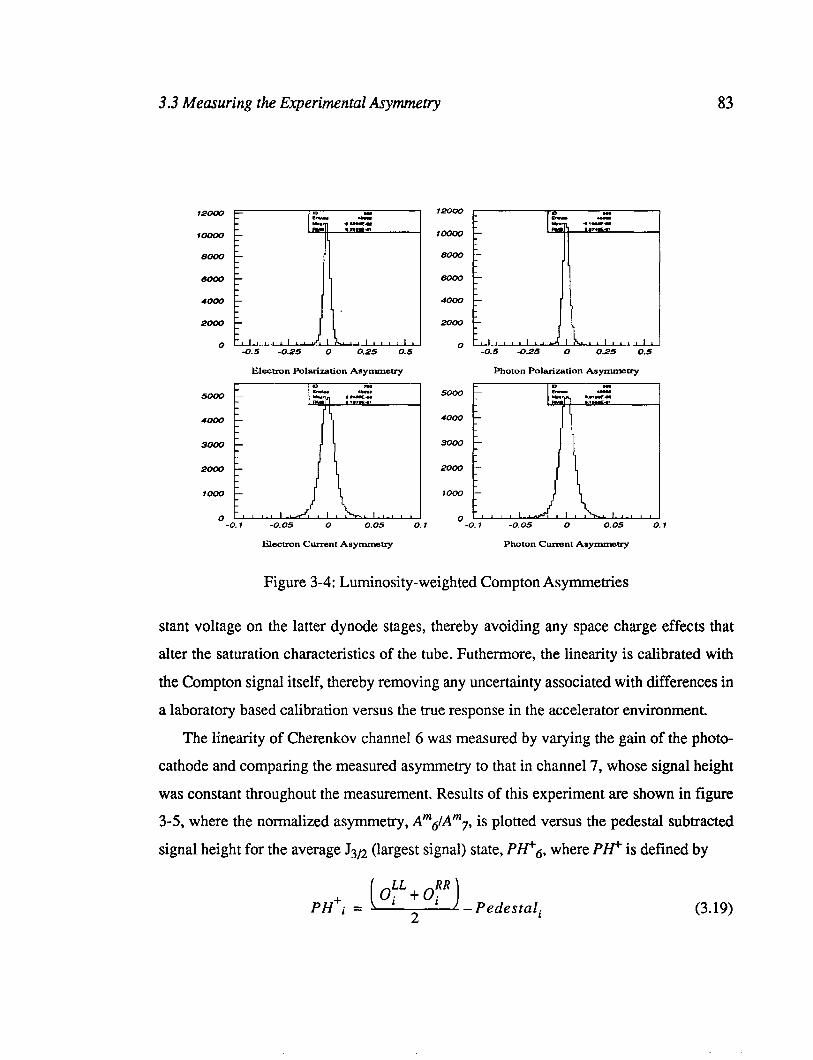
3.3 Measuring the Experimental Asymmetry 83
Boo0 Boo0 - -
6000 6000 - -
4000 4000 - -
2000 2000 - -
0.5 0.5 -0.25 -0.25 0 0 0.25 0.25 0.5 0.5
10000 - , HI1 *17-w
8000 - I
8000 -
4000 -
2000 -
0 ~‘~~t~‘~~J’ L. , , I I 1 I , I , -0.5 -0.25 0 0.25 0.5
Electron Polarization Asymmetry Photon Polarization Asymmetry
:g ,,),,, ,i,i ,,,,,, j
-0.1 -0.05 0 0.05 0.
5000
4000
3000
2000
1000
0 t Photon Cumnt Asymmetry
Figure 3-4: Luminosity-weighted Compton Asymmetries
stant voltage on the latter dynode stages, thereby avoiding any space charge effects that
alter the saturation characteristics of the tube. Futhermore, the linearity is calibrated with
the Compton signal itself, thereby removing any uncertainty associated with differences in
a laboratory based calibration versus the true response in the accelerator environment.
The linearity of Cherenkov channel 6 was measured by varying the gain of the photo-
cathode and comparing the measured asymmetry to that in channel 7, whose signal height
was constant throughout the measurement. Results of this experiment are shown in figure
3-5, where the normalized asymmetry, Amg/Am7, is plotted versus the pedestal subtracted
signal height for the average J~D (largest signal) state, PH+,, where PH+ is defined by
pH+i = LkL?zF.l -Pedestal 2 i (3.19)
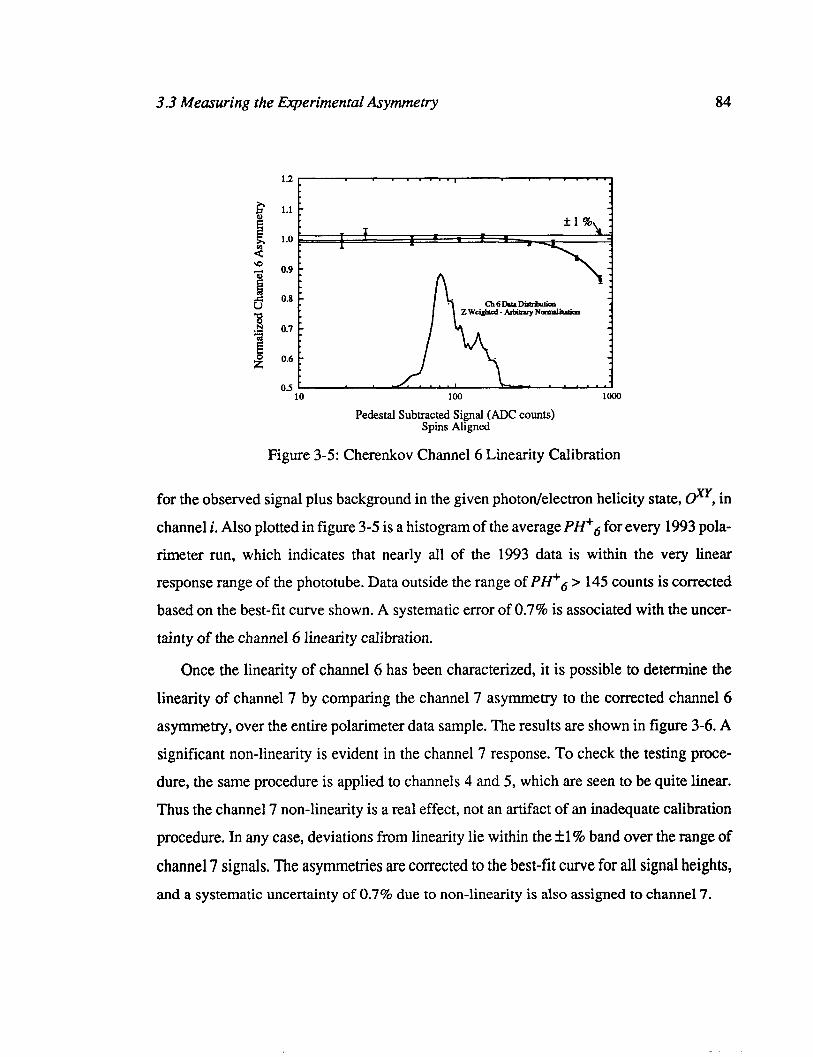
3.3 Measuring the Experimental Asymmetry 84
0.8
0.6
Ch6hhDismh1im ZWeigIued- Arbiumy Nmmliurim
100
Pedestal Subtracted Signal (ADC counts) Spins Aligned
Figure 3-5: Cherenkov Channel 6 Linearity Calibration
for the observed signal plus background in the given photon/electron helicity state, dyy, in
channel i. Also plotted in figure 3-5 is a histogram of the average PH+b for every 1993 pola-
rimeter run, which indicates that nearly all of the 1993 data is within the very linear
response range of the phototube. Data outside the range of PH+6 > 145 counts is corrected
based on the best-fit curve shown. A systematic error of 0.7% is associated with the uncer-
tainty of the channel 6 linearity calibration.
Once the linearity of channel 6 has been characterized, it is possible to determine the
linearity of channel 7 by comparing the channel 7 asymmetry to the corrected channel 6
asymmetry, over the entire polarimeter data sample. The results are shown in figure 3-6. A
significant non-linearity is evident in the channel 7 response. To check the testing proce-
dure, the same procedure is applied to channels 4 and 5, which are seen to be quite linear.
Thus the channel 7 non-linearity is a real effect, not an artifact of an inadequate calibration
procedure. In any case, deviations from linearity lie within the fl% band over the range of
channel 7 signals. The asymmetries are corrected to the best-fit curve for all signal heights, and a systematic uncertainty of 0.7% due to non-linearity is also assigned to channel 7.
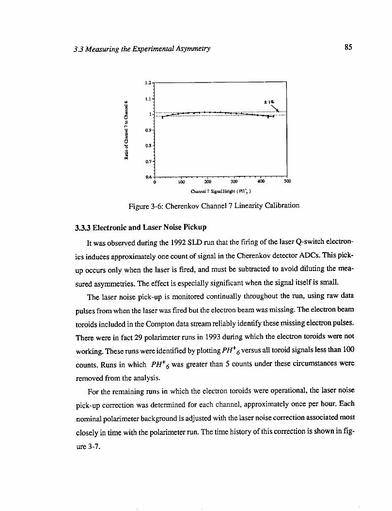
3.3 Measuring the Experimental Asymmetry 85
l.l- \D f 1%
1 6 9 e rt 0.9 -
% 0.8 -
d d
0.7 -
Channel 7 SignalHeight ( PH’, )
Figure 3-6: Cherenkov Channel 7 Linearity Calibration
3.3.3 Electronic and Laser Noise Pickup
It was observed during the 1992 SLD run that the firing of the laser Q-switch electron-
ics induces approximately one count of signal in the Cherenkov detector ADCs. This pick-
up occurs only when the laser is fired, and must be subtracted to avoid diluting the mea-
sured asymmetries. The effect is especially significant when the signal itself is small. The laser noise pick-up is monitored continually throughout the run, using raw data
pulses from when the laser was fired but the electron beam was missing. The electron beam
toroids included in the Compton data stream reliably identify these missing electron pulses.
There were in fact 29 polarimeter runs in 1993 during which the electron toroids were not
working. These runs were identified by plotting PH+, versus all toroid signals less than 100
counts. Runs in which PH+6 was greater than 5 counts under these circumstances were
removed from the analysis.
For the remaining runs in which the electron toroids were operational, the laser noise
pick-up correction was determined for each channel, approximately once per hour. Each
nominal polarimeter background is adjusted with the laser noise correction associated most
closely in time with the polarimeter run. The time history of this correction is shown in fig-
ure 3-7.

3.3 Measuring the Experimental Asymmetry 86
:0
Time (Days since Jan. 1 1993)
Figure 3-7: A time history of the laser noise pick-up for Cherenkov channel 6.
From the local spread of the measurements, we infer a statistical error of approximately
0.3 counts on any given correction. However, the ultimate number of significance in the
A, analysis is the average polarization. This means that only the average correction
directly affects the error on Am, and the error on the average correction shrinks with the
number of measurements, which is on the order of 3000. Therefore the error on the laser
noise pick-up correction has a negligible contribution to the overall systematic error, once
the correction is applied.
Electronic noise arising from channel-to-channel cross-talk has been studied in two
ways: first by searching for signal in all other tubes when only one tube has voltage applied,
and second by searching for signal in one unenergized tube when all other tubes have a volt-
age applied. The first study showed that no unenergized tube measured more than 0.1% of
the signal from the energized channel. The complementary study showed no measurement
greater that 0.5% of the normal signal in an unenergized tube induced by cross-talk from
all other energized tubes. However, the effect of such cross-talk on the measured asymme-
try in a given channel is much smaller. We therefore assign a conservative estimate of 0.2%
systematic uncertainty due to electronic noise.
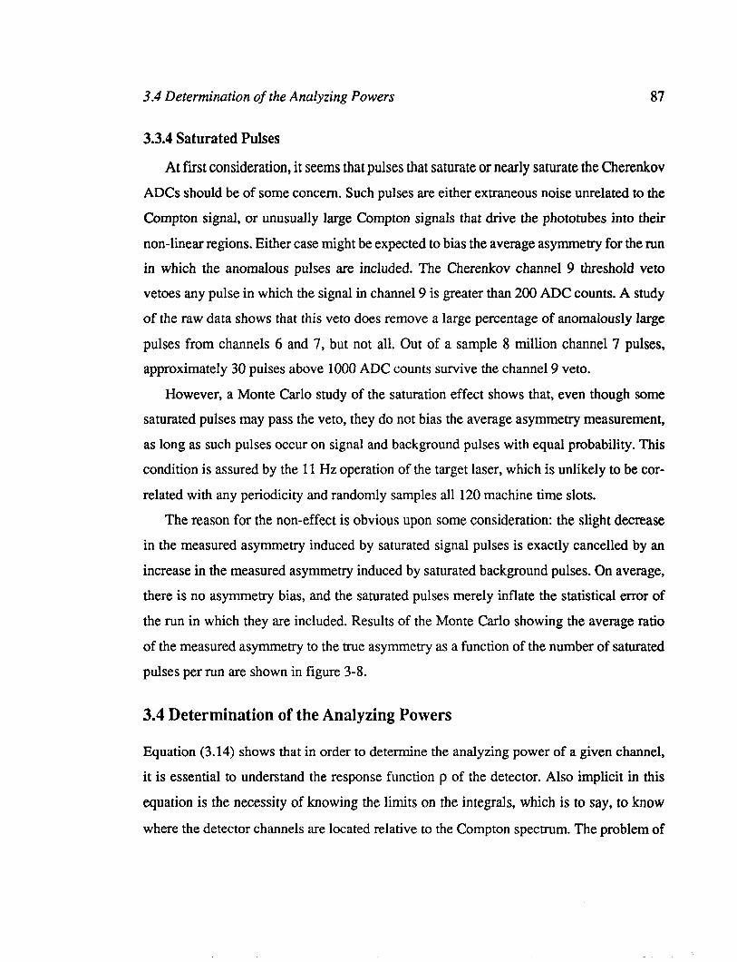
3.4 Determination of the Analyzing Powers 87
3.3.4 Saturated Pulses
At first consideration, it seems that pulses that saturate or nearly saturate the Cherenkov ADCs should be of some concern. Such pulses are either extraneous noise unrelated to the
Compton signal, or unusually large Compton signals that drive the phototubes into their
non-linear regions. Either case might be expected to bias the average asymmetry for the run
in which the anomalous pulses are included. The Cherenkov channel 9 threshold veto
vetoes any pulse in which the signal in channel 9 is greater than 200 ADC counts. A study
of the raw data shows that this veto does remove a large percentage of anomalously large
pulses from channels 6 and 7, but not all. Out of a sample 8 million channel 7 pulses, approximately 30 pulses above 1000 ADC counts survive the channel 9 veto.
However, a Monte Carlo study of the saturation effect shows that, even though some
saturated pulses may pass the veto, they do not bias the average asymmetry measurement,
as long as such pulses occur on signal and background pulses with equal probability. This
condition is assured by the 11 Hz operation of the target laser, which is unlikely to be cor-
related with any periodicity and randomly samples all 120 machine time slots.
The reason for the non-effect is obvious upon some consideration: the slight decrease
in the measured asymmetry induced by saturated signal pulses is exactly cancelled by an
increase in the measured asymmetry induced by saturated background pulses. On average,
there is no asymmetry bias, and the saturated pulses merely inflate the statistical error of
the run in which they are included. Results of the Monte Carlo showing the average ratio
of the measured asymmetry to the true asymmetry as a function of the number of saturated
pulses per run are shown in figure 3-8.
3.4 Determination of the Analyzing Powers
Equation (3.14) shows that in order to determine the analyzing power of a given channel,
it is essential to understand the response function p of the detector. Also implicit in this
equation is the necessity of knowing the limits on the integrals, which is to say, to know
where the detector channels are located relative to the Compton spectrum. The problem of
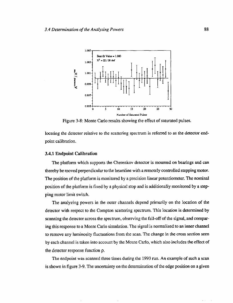
3.4 Determination of the Analyzing Powers 88
Bat-fit Value = 1 .OOO . . X2 -22/28dof
1.003-
~995!....,....,....,....,....,.... 0 5 10 15 20 25
Number of Saturated Pulses
3
Figure 3-8: Monte Carlo results showing the effect of saturated pulses.
locating the detector relative to the scattering spectrum is referred to as the detector end-
point calibration.
3.4.1 Endpoint Calibration
The platform which supports the Cherenkov detector is mounted on bearings and can
thereby be moved perpendicular to the beamline with a remotely controlled stepping motor.
The position of the platform is monitored by a precision linear potentiometer. The nominal
position of the platform is fixed by a physical stop and is additionally monitored by a step-
ping motor limit switch.
The analyzing powers in the outer channels depend primarily on the location of the
detector with respect to the Compton scattering spectrum. This location is determined by
scanning the detector across the spectrum, observing the fall-off of the signal, and compar-
ing this response to a Monte Carlo simulation. The signal is normalized to an inner channel to remove any luminosity fluctuations from the scan. The change in the cross section seen
by each channel is taken into account by the Monte Carlo, which also includes the effect of
the detector response function p.
The endpoint was scanned three times during the 1993 run. An example of such a scan
is shown in figure 3-9. The uncertainty on the determination of the edge position on a given

3.4 Determination of the Analyzing Powers 89
+ +
/
$ •b
0.6 +a
+ 0.4 .
+ I
Distance from Nominal Position (cm)
Figure 3-9: Compton kinematic edge scan.
Date Edge Position (cm) 4/26/93 0.86 f 0.04 5/02/93 0.84 f 0.02 7/15/93 0.87 AI 0.02
Table 3-l : 1993 Endpoint Scan Results
scan is less than 200 microns. The results of the three scans are shown in table 3-l; the
quoted position is the distance from the kinematic endpoint to the inner (closest to the beam
line) wall of channel 7.
3.4.2 Zero Asymmetry Point
It is not sufficient to determine the location of the endpoint at specific times during the
run; we also require a relative position monitor throughout the run in order to bridge the
gap between scans and take into account any potential beam motion that may have occurred during these periods. Such a monitor is provided by following the quantity
A, = A* I I A3-A2
(3.20)
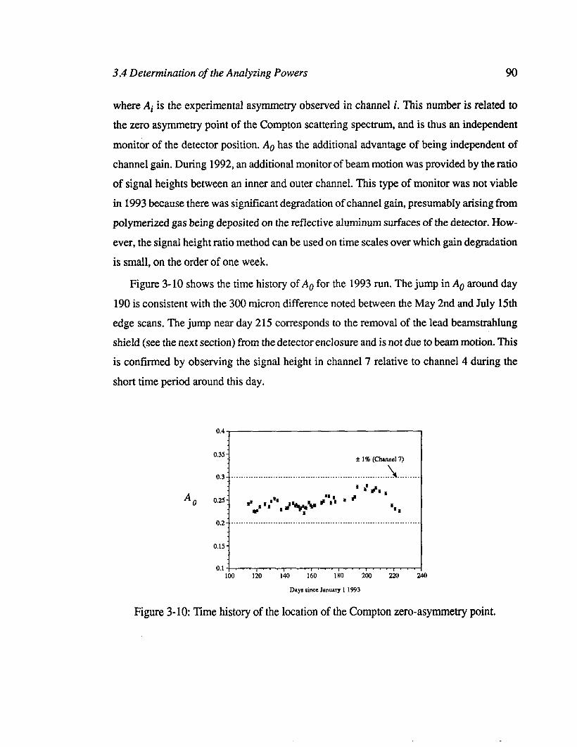
3.4 Determination of the Analyzing Powers 90
where Ai is the experimental asymmetry observed in channel i. This number is related to the zero asymmetry point of the Compton scattering spectrum, and is thus an independent
monitor of the detector position. A0 has the additional advantage of being independent of
channel gain. During 1992, an additional monitor of beam motion was provided by the ratio
of signal heights between an inner and outer channel. This type of monitor was not viable
in 1993 because there was significant degradation of channel gain, presumably arising from
polymerized gas being deposited on the reflective aluminum surfaces of the detector. How-
ever, the signal height ratio method can be used on time scales over which gain degradation
is small, on the order of one week.
Figure 3-10 shows the time history of A, for the 1993 run. The jump in A, around day
190 is consistent with the 300 micron difference noted between the May 2nd and July 15th
edge scans. The jump near day 215 corresponds to the removal of the lead beamstrahlung
shield (see the next section) from the detector enclosure and is not due to beam motion. This
is confumed by observing the signal height in channel 7 relative to channel 4 during the
short time period around this day.
1 f f A, 0.25 f if f
ff f ‘tfff JQ+ ;‘A f l c lff
0.1 .“~“.,‘..,“.,“‘,..‘,.‘. 100 120 140 160 180 200 220 :
Days since January 1 1993
lo
Figure 3-10: Time history of the location of the Compton zero-asymmetry point.

3.4 Determination of the Analyzing Powers 91
Figure 3-10 shows that the beam is position is quite stable between edge scans. The
combination of data from edge scans and the A0 monitor were used to set three calibration
periods, and three sets of analyzing powers were calculated based on the determined posi-
tions during these periods. The results are presented in table 3-2.
Period Calibrated Position a6 a7 4/24 - 7/10 0.84 -t 0.025 0.6151 0.7020 7/10 - 8/4 0.87 f 0.025 0.6118 0.7007
1 8/4 - 9/l 1 0.88 + 0.025 1 0.6107 1 0.7003 1
Table 3-2: Nominal Positions and Analyzing Powers by Period
3.4.3 The Beamstrahlung Shield
For the majority of the 1993 run, a 0.1 inch thick lead shield sat between the innermost
Cherenkov detector channel (channel 1) and the aluminum gas containment cannister of the
detector. This lead was inserted in order to absorb soft radiation from the beamstrahlung
monitor, which is located directly across the beam pipe from the Compton detectors.
During the run, it was discovered that the ratio of the asymmetry measured in a given
channel with the lead radiator in place to that measured with no radiator was slightly higher
than expected. More detailed EGS simulations indicated that the presence of the beam-
strahlung shielding was very likely contaminating the inner detector channels with low
asymmetry showering, because the shielding itself was located very near the minimum of
the Compton asymmetry curve. The extent of the contamination could not be precisely
modeled due to the strong dependence on the shield position and angle, which were not well
known. However, the simulations predicted negligible effects on the asymmetries mea-
sured in the outer channels.
The beamstrahlung shield was removed on July 15, 1993. Comparison of data taken
after the removal versus data taken before the removal agrees with the EGS Monte Carlo
predictions and confirms the hypothesis that the outer channels were unaffected by low-
asymmetry contamination. An upper limit of 0.2% is placed on the uncertainty in the outer
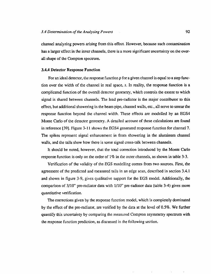
3.4 Determination of the Analyzing Powers 92
channel analyzing powers arising from this effect. However, because such contamination
has a larger effect in the inner channels, there is a more significant uncertainty on the over-
all shape of the Compton spectrum.
3.4.4 Detector Response Function
For an ideal detector, the response function p for a given channel is equal to a step func-
tion over the width of the channel in real space, s. In reality, the response function is a complicated function of the overall detector geometry, which controls the extent to which
signal is shared between channels. The lead pre-radiator is the major contributor to this
effect, but additional showering in the beam pipe, channel walls, etc., all serve to smear the response function beyond the channel width. These effects are modelled by an EGS4
Monte Carlo of the detector geometry. A detailed account of these calculations are found
in reference [39]. Figure 3-l 1 shows the EGS4 generated response function for channel 7.
The spikes represent signal enhancement in from showering in the aluminum channel walls, and the tails show how there is some signal cross-talk between channels.
It should be noted, however, that the total correction introduced by the Monte Carlo
response function is only on the order of 1% in the outer channels, as shown in table 3-3.
Verification of the validity of the EGS modelling comes from two sources. First, the
agreement of the predicted and measured tails in an edge scan, described in section 3.4.1
and shown in figure 3-9, gives qualitative support for the EGS model. Additionally, the
comparison of 3/10” pre-radiator data with l/10” pre-radiator data (table 3-4) gives more
quantitative verification.
The corrections given by the response function model, which is completely dominated
by the effect of the pre-radiator, are verified by the data at the level of 0.5%. We further quantify this uncertainty by comparing the measured Compton asymmetry spectrum with
the response function prediction, as discussed in the following section.
3.4 Determination of the Analyzing Powers 93
Detector Response Function Channel 7
Pb Radiator = 0.762 cm
Pb Shield = 0.0 cm
cm from undeflected beamline
45
40
35
30
25
20
15
10
5
0 76 18 20
cm from undeflected beamline
Figure 3-11: Cherenkov detector response function for channel 7. The first graph does not include the beamstrahlung shield, the second does.
Channel 6
Ideal a
0.6179 Corrected a % difference
0.6107 1.17
I 7 1 0.7120 1 0.7003 1 1.64 1 L I I I I
Table 3-3: Ideal and Corrected Analyzing Powers
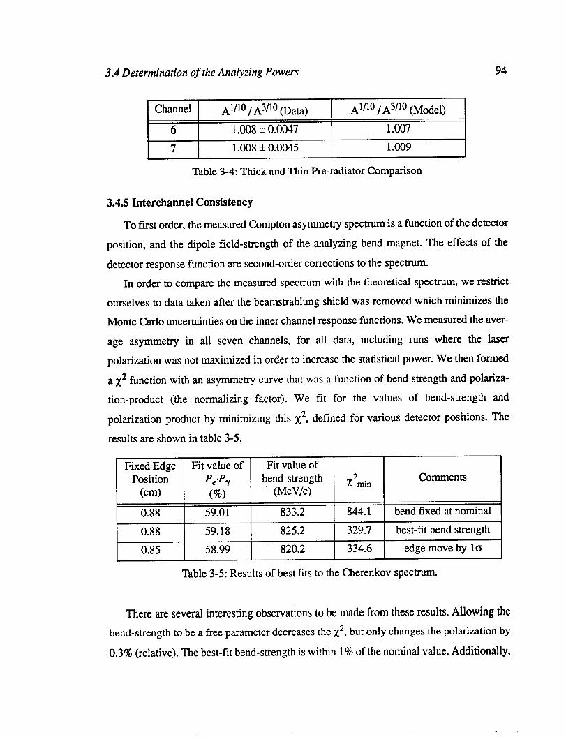
3.4 Determination of the Analyzing Powers 94
Channel
6
A’/” / A3/*0 (Data) 1.008 f 0.0047
A1’lo /A3/lo (Model) 1.007
I I
7 1.008 + 0.0045 1.009
Table 3-4: Thick and Thin Pre-radiator Comparison
3.4.5 Interchannel Consistency
To first order, the measured Compton asymmetry spectrum is a function of the detector
position, and the dipole field-strength of the analyzing bend magnet. The effects of the
detector response function are second-order corrections to the spectrum. In order to compare the measured spectrum with the theoretical spectrum, we restrict
ourselves to data taken after the beamstrahlung shield was removed which minimizes the Monte Carlo uncertainties on the inner channel response functions. We measured the aver-
age asymmetry in all seven channels, for all data, including runs where the laser
polarization was not maximized in order to increase the statistical power. We then formed
a x2 function with an asymmetry curve that was a function of bend strength and polariza-
tion-product (the normalizing factor). We fit for the values of bend-strength and
polarization product by minimizing this x2, defined for various detector positions. The
results are shown in table 3-5.
Fixed Edge Fit value of Fit value of Position pe*p, bend-strength xzrni, Comments
(cm) v4 (MeV/c)
0.88 59.01 833.2 844.1 bend fixed at nominal 0.88 59.18 825.2 329.7 best-fit bend strength 0.85 58.99 820.2 334.6 edge move by 10
Table 3-5: Results of best fits to the Cherenkov spectrum.
There are several interesting observations to be made from these results. Allowing the bend-strength to be a free parameter decreases the x2, but only changes the polarization by
0.3% (relative). The best-fit bend-strength is within 1% of the nominal value. Additionally,
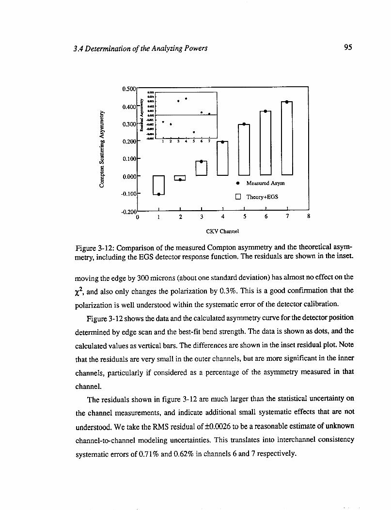
3.4 Determination of the Analyzing Powers 95
-
r-l 0.200 ZL-LJ I 234361
0.100
l Measured Asym
0 Theory+EGS
-0.200’ I I I I I I I J
0 1 2 3 4 5 6 7 8
CKV Channel
Figure 3-12: Comparison of the measured Compton asymmetry and the theoretical asym- metry, including the EGS detector response function. The residuals are shown in the inset.
moving the edge by 300 microns (about one standard deviation) has almost no effect on the
x2, and also only changes the polarization by 0.3%. This is a good confirmation that the
polarization is well understood within the systematic error of the detector calibration.
Figure 3- 12 shows the data and the calculated asymmetry curve for the detector position
determined by edge scan and the best-fit bend strength. The data is shown as dots, and the
calculated values as vertical bars. The differences are shown in the inset residual plot. Note
that the residuals are very small in the outer channels, but are more significant in the inner
channels, particularly if considered as a percentage of the asymmetry measured in that
channel.
The residuals shown in figure 3-12 are much larger than the statistical uncertainty on
the channel measurements, and indicate additional small systematic effects that are not
understood. We take the RMS residual of f0.0026 to be a reasonable estimate of unknown
channel-to-channel modeling uncertainties. This translates into interchannel consistency
systematic errors of 0.71% and 0.62% in channels 6 and 7 respectively.

35 Target Polarization 96
3.5 Target Polarization
The largest systematic error affecting the polarimeter is the determination of the circular polarization of the target laser at the Compton interaction point, Py The problem is that the
CW is inside the SLC vacuum and analysis optics cannot be placed there. Pr is measured
at two other points: on the optics bench, after the beam has been circularly polarized, and
in the analysis box, after the beam has exited the SLC vacuum. However, phase shifts
induced by the laser transport optics prevent either of the monitors from directly measuring
P, A complete description of the 1993 Compton target polarization determination is found
in Reference [53], the highlights of which are presented in this section.
3.5.1 Optics
At this point, a brief clarification of some classical optics is called for. A monochro-
matic, coherent packet of arbitrarily polarized (also called elliptically polarized) photons
can be described by the superposition of linear polarizations about orthogonal axes:
Z(t) = Ex [I = EY Axei~‘el”xt - -1 pyeiwtei~yt
(3.21)
where E is the electric field, t is time, o is the classical frequency of the light, and ~x,~ are
the absolute phases of the x and y components. The light is considered linearly polarized
when the phase difference between the x and y components of the electric field vector, A<p
(= <px - cp,), is zero. The light is considered circularly polarized if Acp = 7r/2 and the mag-
nitude of each component is equal, that is, A, = A,. This state has a physical interpretation
in terms of photons: it is the one in which all photons in the bunch are in the same helicity
eigenstate. The circular polarization (i.e. the degree to which the light is in a helicity eigen-
state) for the arbitrary light described in equation (3.21) is given by
ReCExl~m~Eyl --Im~E,)ReWyl P, = 2.
lEx12 + lEY12 (3.22)
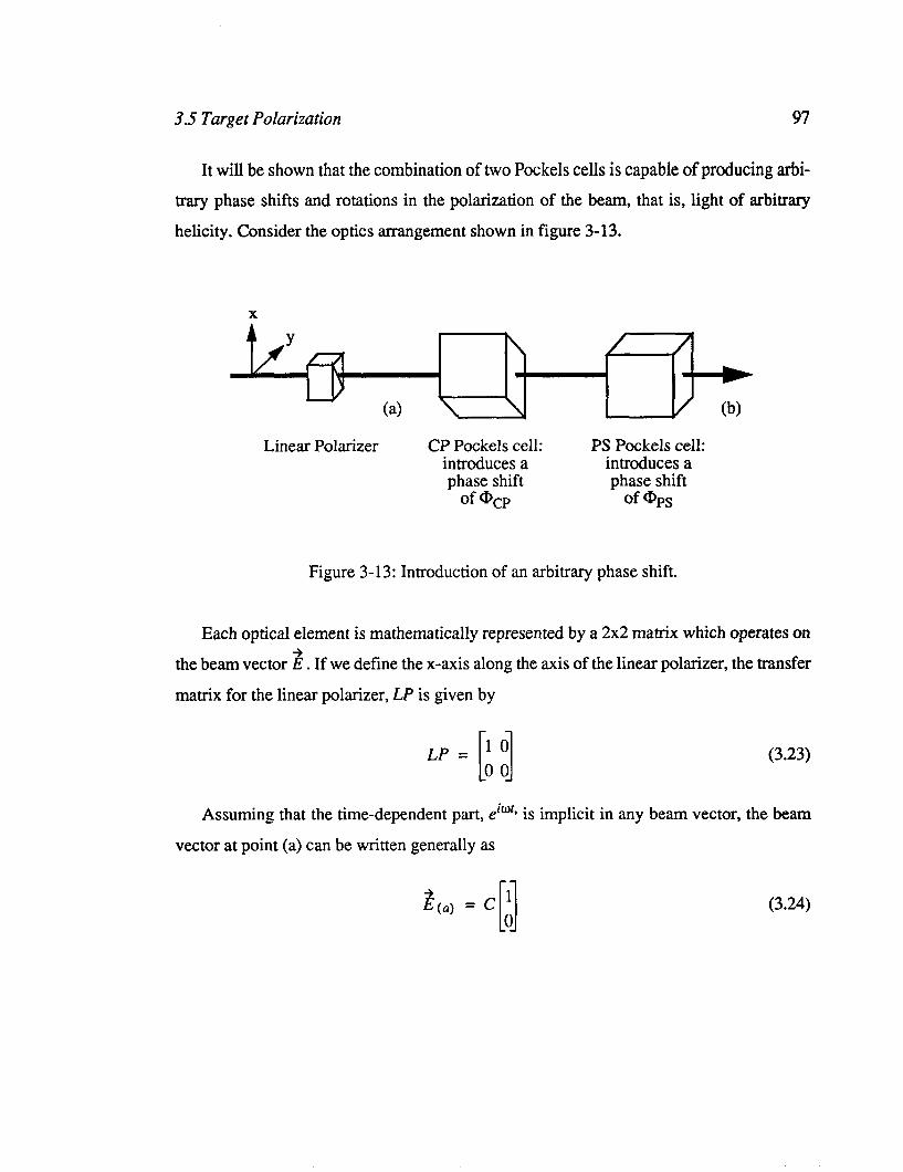
3.5 Target Polarization 97
It will be shown that the combination of two Pockels cells is capable of producing arbi- trary phase shifts and rotations in the polarization of the beam, that is, light of arbitrary
helicity. Consider the optics arrangement shown in figure 3-13.
Linear Polarizer CP Pockels cell: introduces a phase shift
of %P
PS Pockels cell: introduces a phase shift
of- QPS
Figure 3-13: Introduction of an arbitrary phase shift.
Each optical element is mathematically represented by a 2x2 matrix which operates on
the beam vector 2. If we define the x-axis along the axis of the linear polarizer, the transfer
matrix for the linear polarizer, LP is given by
LP= ;; [I
(3.23)
Assuming that the time-dependent part, eior* is implicit in any beam vector, the beam
vector at point (a) can be written generally as
2 (a) = c 1 [I 0 (3.24)
3.5 Target Polarization 98
The CP Pockels cell has its principle axes aligned 45’ with respect to the linear polar- izer axis (the x-axis). Therefore its effect on the beam vector, represented by the matrix CP,
is given by
CP =
7c 7t cos- -sin- 4 410 L I[] lr n Oe i@CP
sin- cos- 4 4
where the rotation matrices are shown explicitly. The PS Pockels cell has its principle axes
aligned with the x-y axes, so its transformation matrix, PS, is simply given by
1 0 PS = [ 1 o ei%, '
The beam vector at point (b) is therefore
&I = (PS) (CP) &u)
(3.26)
(3.27)
Thus the CP Pockels cell controls the relative amplitude of the x-y components, and the PS
Pockels cell controls the relative phase between the components (Acp = (I$$. The circular
polarization of this light is calculated through equation (3.22) to be
pY = sinDcPcos<DPS. (3.28)
3.5.2 Pre-AUTOPOCKSCAN Analysis
At the beginning of the 1993 run, we took the following approach: An intrusive mea-
surement was made at the Compton IP by breaking the SLC vacuum. Pr was found to be
(98 f l)%. It was then assumed that the transport line phase shifts were constant in time.
Under this assumption, the analysis box optics could measure the stability of P, although
not Pr itself. This period of time during which this assumption was the basis of the laser
light analysis is now called the pre-AUTOPOCKSCAN era, which lasted through April 27,
3.5 Target Polarization 99
1993. All running beyond this date is referred to as the AUTOPOCKSCAN era, which is described in the next section.
As it turns out, the phase shifts induced by the laser transport system were not constant in time. This fact is illustrated in figure 3-14, which is a time history of the laser polariza-
tion measured in the analysis box, PrAB, for the first forty days of the 1993 run. This era is
divided into seven epochs, based on the stability of the asymmetry measurements. The
jumps in PyAB during a given epoch do not correspond to any changes in the measured
Compton asymmetry and are therefore due to changes in the transport line phase shifts
rather than real changes in Py The larger jumps were probably a result of optical damage
(or the replacement of damaged optical components) caused by laser “hot-spots” (points of
unusually high intensity within the beam profile). These hot-spots were in turn caused by
a failing Q-switch mechanism in the laser head, which was eventually replaced. The small
jumps (between epochs II and III for instance) are probably related to Pockels cell align-
ment, and may also be related to environmental factors such as temperature.
During the first three epochs of this era, there was only one Pockels cell (the CP cell)
installed on the laser bench. However, between epochs II and III the principal axes of this
cell were rotated by 45’. This means that the combination of the manual voltage scans taken
in each of these two eras actually serves to map the phase shifts along two orthogonal axes,
and thus an overall Pu for the two eras is determined. (The method by which Pu is deter-
mined through Pockels cell voltage scans is described in the next section.)
Starting with epoch IV, the PS Pockels cell was installed on the CLS laser bench. Man-
ual voltage scans of both cells in epochs IV, V, and VI, allow determinations of P, for each
of those epochs. Automated scans were implemented at the end of epoch VII, and because
there were no optics or transport line changes between epoch VII and the start of the scan-
ning era, the determinations made during the first auto-scans are projected backward in
time to include epoch VII. A summary of the P, determinations and methods used for this
era is given in table 3-6.
The systematic error on all Pr measurements in the pre-AUTOPOCKSCAN era is esti-
mated to be 2.1%. Approximately 27% of all Z data was taken during this era.

3.5 Target Polarization 100
0.65
0.6
Prescan ETOZ Analysis Box Light Polarization. Diode 1 Prescan ETOZ Analysis Box Light Polarization. Diode 1
((ARl-ALl)/(ARl+ALl)) VS ST Days Since January 1.1993
Figure 3-14: PyM in the Pre-AUTOPOCKSCAN era.
Epoch
I II
P, 0.98 0.96
Method by which Py is determined
Intrusive direct measurement at CIP Manual scan of CP phase
III 0.96 Manual scan of PS phase IV 0.93 Manual scan of both cells
V 0.99 Manual scan of both cells
VI 0.97 Manual scan of both cells
VII 0.99 Automated scanning implemented -
Table 3-6: P, measurements during the pre-AUTOPOCKSCAN era.

3.5 Target Polarization 101
3.53 AUTOPOCKSCAN Analysis
Once the phase shift instability of the transport optics became apparent, a new strategy
for monitoring said phase shifts and measuring P, was implemented. This strategy involves
two different types of automated scanning: one in which the Pockels cell voltages are
scanned versus the measured Compton asymmetry (EPOL scan), and the other in which the
voltages are scanned versus the analysis box photodiode signals (LP scan). EPOL scans
allow us to determine how far from the maximum achievable polarization we are at a given voltage setting. LP scans allow us to determined the value of the maximum achievable
polarization. Only the combination of both types of scans allows an absolute measurement
of Py for a given time period.
Nominal voltages on the Pockels cells are defined by those voltages which maximized
the Compton asymmetry during a previous scan. In both types of scans, the voltages on
each Pockels cell are scanned independently, that is, one cell is held at nominal voltage
while the other cell is scanned (Voffset = +800, f600, &400, and &200 volts) beyond its nom-
inal setting. When the CP cell was scanned, it voltage was flipped pseudo-randomly during
each run between &(V%,,, +VorrseJ, while the PS cell was held at its nominal voltage.
When the PS cell was scanned, the CP cell alternated between f(VCPnom& while the PS cell
was set to (VpsnOm~,+VOK~et).
EPOL scans take place continually. The cell voltages are set, and a normal 20,000 event
Compton run is taken. A nominal run (i.e. both cells set to nominal voltages) is taken in
between each pair of scan points. That means (2 cells)x(4 voltage offsets)x(3 voltage set-
tings per offset [&Voflsti and Vnominal 1) = 24 runs per scan, which takes slightly more than one
hour to complete. During this time, eight nominal runs are taken, approximately one nom- inal run every eight minutes.
At the end of each EPOL scan, an LP scan is scheduled. The LP scan consists of eighty
points, forty scanning the CP voltages and 40 scanning the PS voltages. Each point consists
of 100 beam crossings, therefore the total length of the scan is 8000 beam crossings, or just over one minute.

3.5 Target Polarization 102
A combination of off-line best-fits to the two types of scans determines P, The photo-
diode signals measured during an LP scan, PDki, during which the Pockels cell voltages are
set to v’cp and V’ps, are fit to the following function
PLI: = G*[1+~~sin[(“~~~“)~]cos[[‘~~~~)~]) (3.29)
Here, the “+” (,‘-“) photodiode is defined to be the one which sees a large signal with a pos- itive (negative) voltage on the CP Pockels cell. G is the gain of the photodiode, U is the
fraction of unpolarized light in the laser beam, and the QAB are the uncompensated phase
shifts along the CP and PS axes observed in the analysis box, in units of volts.
There are two phases of LP scan analysis. During the first phase, the unpolarized frac-
tion U is set to zero, and aA’ and Vu4 are free parameters of the fit. During the second
phase, all variables except U are fixed, and U is determined by fitting only the data very
near the minimum of the photodiode extinction curve. This is done because all information
on the unpolarized fraction, which is related to the deviation of the minimum from zero,
comes from points in this neighborhood, and because the fit convergence improves greatly
with this restriction.
EPOL scans are fit to the following function
A Ti = (P,P,) sin[[ “zF]:]cos[( v”;,F);] (3.30)
where the measured asymmetry Am is as defined in equation (3.13) and the polarization
product is a single parameter. For this fit the quarter-wave voltages are fixed at the values
determined by the most recent LP scan. The 0”’ represent the uncompensated phase shifts
at the Compton interaction point. Note that as the Qc” become larger, the uncertainties on
the Qc” have a greater effect on the determination of Py For this reason, the nominal volt-
ages were reset by polarimeter experts whenever either Qc” > 200 V. Ideally, we would nominal set V,,
CIP = vy’p” + a,,
nominal and VP, = @gP at the end of each EPOL scan, but this

3.6 Absolute Sign Determination 103
is not possible without on-line fitting and would be dangerous because of the possibility of
a bad fit setting the voltages far away from the true nominal.
The laser polarization from a set of LP and EPOL scans is now given by
p, = (1-U)sin [ ( v:mi;;je-j] cos [ ( Gmi;;~4Y);] (3.31)
where the quarter-wave voltages are determined by the first phase of the LP fits, U is deter- mined by the second phase of the LP fits, and the iDc” are determined by the EPOL fits.
Figure 3-15 shows the time history of all Pr measurements in the AUTOPOCKSCAN
era. Approximately 73% of the Z data was taken during this time period. The systematic
uncertainty on P, during this era is 0.6%.
: . .
e 0.96
t l
140 160 180 200
Time (Days since Jan. 1 1993)
Figure 3-15: Time history of P, during the AUTOPOCKSCAN era.
3.6 Absolute Sign Determination
The determination of the absolute sign of the electron polarization is of course essential to the Am analysis, since Am requires counting the number of left and right-handed Zs. Recall
3.6 Absolute Sign Determination 104
from equation (3.13) that the measured asymmetry is equal to the product of the laser polar-
ization, the electron polarization, and the analyzing power Given these inputs, we have
sufficient information to determine the sign of the electron polarization. We have discussed
the asymmetry measurement in section 3.3. The analyzing power is calculated from the the-
oretical Compton asymmetry, this sign of which is discussed below. The absolute target
helicity is monitored on a pulse-by-pulse basis, and is also described in this section.
3.6.1 Sign of the Compton Scattering Asymmetry
In 1992, there was a period of excitement due to the fact that the measured value of A,
was negative, contrary to the expectations of the Standard Model. This discrepancy was
traced to a theoretical error on the sign of the Compton scattering asymmetry. Most refer-
ences deftly avoid mentioning the sign of the asymmetry, and of those that do make a claim,
some are incorrect. The correct result is that fully backward Compton scattering (corre-
sponding to the Compton kinematic endpoint) has a larger cross section when the electron
and photon helicities are parallel [52].
This result can be understood through the following argument: Consider the high-
energy limit of fully-backward Compton scattering, when both the electron and photon
exist in helicity eigenstates. Given that the longitudinal component of angular momentum,
j,, must be conserved, it follows that the spin direction of the electron and photon in the
final state must be the same as in the initial state. This means that the helicities of the photon
and electron will change sign. If angular momentum is also conserved at each vertex of the
exchange diagrams (figure 3-l), it also follows that the& = 3~ initial state must be prefer-
entially occur through the u-channel exchange, while the j, = I/2 initial state must
preferentially occur through the s-channel diagram. All that remains to be seen is that the
contribution from the u-channel, whose propagator (in the denominator) is proportional to
the electron mass-squared, is greater than the s-channel, whose propagator is proportional
to the center-of-mass energy-squared.
To summarize, for fully backward scattering, the u-channel dominates the s-channel,
and only thej, = 3~ state contributes to the u-channel. Therefore, the state in which the inci-

3.6 Absolute Sign Determination 105
dent photon and electron helicities are parallel (corresponding to thej, = 3/2 state) has the
larger cross section at the Compton kinematic endpoint.
3.6.2 Helicity of the Target Photons
A quarter-wave plate is an optical element which, for a given wavelength, imparts 90’
of phase advance for fields projected along the fast axis relative to those along the slow
axis. In order to measure the helicity of polarized light, one requires a quarter-wave plate
with an identified slow axis. In 1992, the PLS and CLS quarter-wave plates were calibrated
by several optical techniques, which are discussed in detail in Reference [54], and are
briefly described below.
Fresnel Total Internal Reflection
This method relies on the fact that after a total internal reflection, the components of linear polarization parallel and perpendicular to the plane of reflection undergo different
phase shifts. This is considered the primary method of quarter-wave plate calibration
because the results are derived from first-principles [55]. Subsequent techniques rely on
commercial optics equipment and standards.
. . ircular Dtchroism
This technique relies on the fact that certain materials in solution preferentially transmit
one handedness of polarized light. We used a standard reference solution of cyano-cobal-
amin (vitamin B-12) and a commercial circular-dichroism spectropolarimeter at a Stanford
biochemistry laboratory, and tested four quarter-wave plates.
Berek Comnensator
A Berek Compensator is an adjustable retarder plate consisting of a single birefringent
crystal (MgF2) whose slow axis is oriented perpendicular to the plate surface. At the proper
setting, the Berek Compensator acts as a quarter-wave plate with an identified slow axis,
and such a quarter-wave plate can be used to find the slow axis of a second quarter-wave
plate. Two of the CLS quarter-wave plates were tested in a commercial laboratory using
this technique.

3.6 Absolute Sign Determination 106
Liauid Crvstal Polarizer
Each of the above slow-axis determinations agreed with the other, as well as with the
manufacturer’s marking of the slow axis, on those plates that had unambiguous markings.
From this extensive research came a relatively simple tool for photon helicity determina-
tion: the liquid-crystal polarizer, or LCP technique.
A liquid crystal polarizer is a commercial device that transmits light of right-handed
helicity and reflects light of left-handed helicity with an extinction ratio of several hundred
to one. In 1992, two LCPs purchased by SLAC were used to test quarter-wave plates, and
agreed with the previous calibrations. In 1993 a LCP optimized to the Compton laser wave-
length was installed on the optics bench to provide a continuous monitor of the light
helicity. Because all light transport between the laser bench and the Compton interaction
point involves mirror pairs mounted in mirror boxes (discussed in section 2.3.1), it is guar-
anteed that there are an even number of reflections between these points. Since each single
reflection changes the handedness of the polarization, it therefore follows that the handed-
ness at the CIP must be the same as that measured on the bench. A study of the LCP
photo&ode signals for the entire run shows that the CLS 01 state corresponded to the right-
handed photon state, and that the meaning of this assignment never changed.
Given this information, it is possible to infer the electron beam helicity assignments for
the entire run, given the sign of the measured Compton asymmetry at the kinematic end-
point (measured by Am,). The sign of Am7 changed only once during the run, on June 10,
1993. This corresponded to the time at which the current on the LTR solenoid was reversed,
changing the orientation of spins in the damping ring, and reversing the meaning of the CLS
helicity assignments.
Era CLS 01 state corresponds to this helicity:
sign of PLS Olstate corresponds to Ae7 this helicity:
I
4/10 - 6/10 1 I
6/10-9/l 1
R
R
I I
negative R 1 I I
positive L
Table 3-7: Inferred Electron Helicity during 1993 run

3.7 Polarimeter Data Selection 107
Changing the sign of the LTR solenoidal field is one of many methods by which sys- tematic errors affecting Am may be reduced. Future experiments may benefit by more
frequent reversals of this type. The LCP provides a simple and safe monitor of the PLS and
CLS helicity assignments, which will change when such reversals are made.
3.7 PoIarimeter Data Selection
The operation of the polarimeter has been described in chapter 2. The important details are
the following: data for each Cherenkov channel are acquired in twelve histograms, based
on 3 possible electron beam states (left polarized, right polarized, and unpolarized) and 4
possible Compton target states (left polarized, right polarized, unpolarized, and off). A typ-
ical polarimeter run consists of 20,000 beam crossings, or approximately three minutes of
live beam time. Runs may be cut short by loss of the electron beam or operator overrides.
At the end of each run, a number of run-stable quantities are read, such as detector voltages
and detector position, and are included in the data structure for the run.
The data are required to satisfy a number of run-specific and channel-specific selection
criteria. Every run must pass all run-specific cuts in order to be included in the analysis. If
neither channel 6 nor channel 7 passes all of the channel-specific cuts then the run is
dropped from the analysis. If both channels 6 and 7 pass all of the channel-specific cuts,
then the polarization for the run is the average measurement for the two channels (this has
the effect of lowering the total systematic error; refer to the following section). Otherwise
the measurement is reported only for the channel that passed all of the channel-specific
cuts.
Runs which pass all run-specific cuts and have at least one channel that passes the chan-
nel-specific cuts form a data set from which the luminosity-weighted polarization, (Pz) ,
is calculated.

3.7 Polarimeter Data Selection 108
3.7.1 Run-specific Cuts
Number of Events
We require at least 100 events in each of the four possible helicity combinations of elec-
trons and photons (LL, RR, LR, RL). This cut primary assures that the calculated statistical
error on the run is valid, and also removes the operator “one-shots” (test runs with the run
length set to 100) at an early stage of the analysis.
Nominal Runs
Only runs during which the CLS Pockels cells are set to their nominal voltage are
included in the polarimeter analysis. During the automated Pockels cell scanning era, a only
one-third of the total polarimeter data were taken at nominal voltages. The systematic error
on the determination of the laser polarization is smallest for nominal runs, because these
runs occur at points where the derivative of the EPOL fit function [equation (3.29)]
approaches zero. We could include all off-nominal runs and their corresponding Pr deter-
minations, but there is nothing to gain by this except an inflated systematic error, since we
are in no way statistically limited by the number of nominal runs (again a result of needing
to know only the average polarization for the entire run). Pockels cell nominal voltages were determined based on database entries and a careful
reconstruction of Polarimeter logbook entries. The nominal voltages were checked by
observing the continuity (in the mathematical sense) of the polarimeter data. Eras during which the incorrect nominal voltages were asserted would appear as gaps of no data or data
with anomalously low polarization.
Veto Status
We require that the electron toroid veto was set, which is to say, we require that miss-
ing-electron pulses were not summed in the histograms of the run in question (vetoes in
general were described in section 2.3.4). Because the beam helicity code for the electrons
is based on the electron source, and has no information about whether the electrons were
dumpered at the end of the linac, runs for which the toroid veto was not operational would

3.7 Polarimeter Data Selection 109
erroneously include the missing-electron pulses in one of the four signal states. This would
effectively lower the measured asymmetries and thus the extracted electron polarizations
for such runs.
Lead Pre-radiator Status
We require that there be 2/10”, 3/10”, l/3”, or 1” of lead pre-radiator in front of the
Cherenkov detector, as these are the thicknesses for which the Cherenkov analyzing powers
have been calibrated. At this point in the analysis, the base analyzing powers are selected
for the given pre-radiator configuration and calibration era.
Detector Position
We require that the detector platform be within 1.36 mm of its nominal position. Within
this range, the base analyzing powers are corrected for any deviation from the nominal
position. Any runs with the platform outside of this range are dropped.
3.7.2 Channel-specific Cuts
Signal-nlus-Background
The average signal plus background must be greater than 35 counts. This cut eliminates
runs in which the laser noise pick-up correction becomes very significant.
The Snin-aligned Pedestal-subtracted Signa! (PH+)
This quantity is required to be greater than 40 and less than 440. The linearity of both
channels has not been measure with sufficient statistics below PH+ < 40. The uncertainty
on the linearity corrections was deemed too large for PH+ > 440. Channel 7 asymmetries
are corrected to the measured linearity curve for 40 < PH? c 440. Channel 6 asymmetries
are corrected when 150 < PH+ < 440.
3.7 Polarimeter Data Selection 110
Statistical Error
The statistical error on the measurement of a given state is given by
(JXy = $( “~~12-[~]2)+~~~2~ [,% I*’ (3.32)
\ / where 0,” is the ith observation of signal-plus-background in the XY state, F is the total
number of signal observations in that state, Bjx is the jth observation of background in the X state, and ZVBx is the total number of background observations in the X state. The domi-
nant statistical effect in the 1993 polarimeter was the intensity-jitter of the target laser. Thus
the variance of the signal-plus-background is much greater than the variance of the back-
ground alone. Additionally, the background was measured much more often than the
signal; on average, ND’ = 20JVxy. Therefore the statistical error on a background measure-
ment makes a negligible contribution to the statistical error for a run.
The polarization product measured by a given channel i, PP, is given by
( 1 A:! PP, = P,P; i = -;;I
i
where the experimental asymmetry and the analyzing power were defined earlier in this
chapter. It follows from equations (3.13) and (3.33) that the statistical error on the polaxiza- PP tion product, pi is given by
PP CTi =
[oy]” + [of”]’
Ny+N;R+Ny+N$
The statistical error on the polarization product is required to be less than 3% absolute in
order for the run to be included in the calculation of the luminosity-weighted polarization.
Note that, as the luminosity-weighted polarization is a weighted average of over 20,000
polarimeter runs, the statistical error on an individual run is irrelevant, and the statistical error on the luminosity-weighted polarization is negligible compare to the systematic error.
3.8 Polarimeter Systematic Errors 111
3.7.3 The Final Compton Polarization
If a polarimeter run has passed the data quality cuts, the polarization product is calcu- lated from the measured Compton asymmetry, as indicated in equation (3.33). The laser
polarization is then read from a database. If the polarimeter run occurs during the pre-scan
era, the laser polarizations are drawn from table 3-6. If the run occurs during the scan era, the laser polarization measurements (shown in figure 3- 15) are searched, and the determi-
nation made closest in time to the polarimeter run is applied to the polarization product, in order to extract the final Compton polarization, P,‘.
3.8 Polarimeter Systematic Errors
To summarize the systematic errors discussed in this chapter:
The detector calibration error reflects the uncertainty of the location of the detector rel- ative to the Compton spectrum, and includes the error on an edge scan determination and
the drift in electron beam position between edge scans. The interchannel consistency error
reflects the uncertainty on the shape of the measured asymmetry, and includes contribu-
tions from the uncertainty in the analyzing bend magnet field strength and the detector
response function simulation. As each channel makes and independent asymmetry mea-
surement, this error is uncorrelated between channels. The linearity uncertainty reflects the
statistical limit on the measurement of the asymmetry versus pulse-height curves. Because the channel 7 linearity curve relies on a normalization to the corrected channel 6 data, these
uncertainties are partially correlated between the two channels. The inner shielding uncer-
tainty is an upper limit on low asymmetry background contamination coming from the
beamstrahlung shield. The electronic noise uncertainty is an upper limit on electronic cross-
talk between channels. The laser polarization error is the weighted mean of the 0.6% error
on the laser polarization during the automated Pockels cell scanning era and the 2% laser
polarization determination during the pre-scan era.
Contributions to the total polarimeter systematic error are summarized in table 3-8. Note that there is indeed an advantage to the averaging of channel 6 and channel 7 polar-
ization measurements, which brings the total systematic error down to 1.3%.

3.9 The Luminosity-weighted Polarization 112
Laser Polarization 1.00 1.00 1.00 1.00 TOTAL: 1.52 1.41 1.33
Table 3-8: Total Systematic Error for Individual Channels and Combined Channels
3.9 The Luminosity-weighted Polarization
It was shown in chapter 1 that the measurement of Am depends only on the luminosity- weighted polarization, (P,) . We estimate this value through the following relation
(3.35)
where Nz is the total number of 2s observed, and PC is the polarization measurement most
closely associated in time with the ith 2. We will discuss the selection of 2s in the next
chapter; taking the 2s as given, the time history of PC is shown in figure 3-16 (A).
The one-dimensional projection of this time history is shown in figure 3-16 (B). The
luminosity-weighted Compton measured electron polarization for the 1993 run is
(P;) = 0.6190 & 0.0082 (3.36)
where the quoted error is purely systematic.
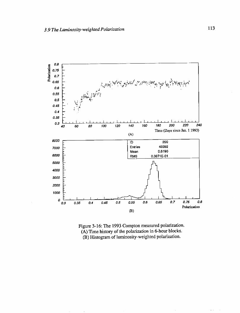
3.9 The Luminosity-weighted Polarization 113
” ” ” ” ” ” ” ” ” ” ” ” ” ‘I”’ I I I I I 1 1 1 40 60 80 103 120 740 160 180 200 220 240
Tie (Days since Jan. 1 1993) (A)
8000 \ ID 200 7000 r Entries 49392
Mean 0.6190 woo - RMS 0.3671 E-01
5000 -
4000 r
3000 -
2000 -
1000 -
0 I I I I 0 I I 0.3 0.35 0.4 0.45 0.5 0.55 0.6 0.65 0.7 0.75 0.8
Polarization 03
Figure 3-16: The 1993 Compton measured polarization. (A) Time history of the polarization in 6-hour blocks. (B) Histogram of luminosity-weighted polarization.
Chapter 4
Z Event Selection and Background Estimation
This chapter will provide the details of the 1993 event selection strategy and background
estimation. The analysis presented is unique in that it depends on calorimetric data only; no
tracking is required. The calorimeter has a large acceptance (up to case = 0.98), and a large
livetime, because the calorimeter triggers can be read out in less than a single SLC cycle
(8.3 ms). As a result a high overall detection efficiency (approximately 94%) is obtained.
The Am measurement does not have particularly stringent event selection require-
ments. Because A, is independent of the final state of the 2 decay, we can accept almost
any produced Z event. The exception is the electron-positron final state, also referred to as
the Bhabha final state. This is the dominant background in the measurement. Other back-
grounds to be considered are: beam-related background events, muon halo events, cosmic-
rays, and so-called “two-photon” events.
4.1 The LAC Energy Scale
In order to describe the event selection criteria, we must first discuss the calibration of the
calorimeter energy scale. The signal size that is associated with a LAC tower is converted
114

4.2 Event Triggers 115
into an energy based on the minimum ionizing energy scale (or ~1 scale), This scale is based on the assumption that the charge deposited arises from a minimum ionizing particle that
loses energy in the lead and liquid argon.
The ~1 scale conversion factors were determined by normalizing the minimum ionizing
peak, seen in the LAC EM sections from tracks in hadronic events, to the expected value [56]. These conversion factors are 2.28~10~~ GeV/ADC count in the EM sections and 5.99~10~~ GeV/ADC count in the HAD sections. All energies discussed in the event selec-
tion criteria of this chapter are defined in terms of this minimum ionizing scale.
The LAC is a sampling calorimeter, which means the total energy passing through the
calorimeter is not measured. Some energy is absorbed by the radiator plates themselves,
and what fraction of the total energy is sampled is a function of the shower type. For
instance, hadronic showers can lose energy through neutrons in hadronic showers, neutri-
nos in pion decay, and also through nuclear binding energy in hadronic production.
Therefore the ratio of the hadronic energy scale (the 71: scale) to the p scale, X/P, is less than
one. Similarly, in electromagnetic showers, the very soft (low momentum) shower products
have a lower efficiency for charge conversion in the calorimeter. Some of this energy is not
sampled, and the ratio of the electromagnetic energy scale to the minimum ionizing scale,
e/v, is also less than one.
Because of these different mechanisms of energy loss, the ratio of the electromagnetic
to hadronic energy scales, e/x, is not equal to one. An analysis of the 1992 data [57] mea-
sures this ratio to be approximately 1.7. As a result, leaving calorimeter energies in the p
scale means that there is a greater separation between purely electromagnetic final states
(e+e-) and hadronic final states. This is actually an advantageous situation for reasons dis-
cussed in section 4.4.1.
4.2 Event Triggers
It is clearly not feasible to write out the state of the SLD detector for every beam crossing. We must have some criteria by which the large quantity of noise is ignored while still writ-

4.2 Event Triggers 116
ing a large percentage of real Z events to tape. One of the most pervasive sources of noise
in the SLD detector are the beam halo muons.
4.2.1 Muons
When off-course electrons or positrons scrape any material in the transport lines, they
can create high energy photons, which may in turn scatter from nuclei to create muon pairs
or pions which decay into muons. These muons (called beam halo muons) can be trapped
in the beam transport at large radii and accompany the parent beam all the way to the SLC
interaction point. They then pass through the SLD parallel to the beam line and deposit
energy in both the endcap and barrel sections of the LAC.
A selection of luminosity monitor triggers is used as a luminosity-weighted random
sample of LAC backgrounds, in order to estimate the muon rate and create an SLC muon
pattern recognition algorithm [58]. Since the halo muons travel parallel to the beam axis,
they can deposit several GeV in the calorimeter, but distributed over many towers. The typ-
ical muon energy distribution is around 20 to 30 ADC counts per tower. The LAC
ENERGY trigger takes advantage of these characteristics in order to minimize the number
of events triggered by beam halo muons.
4.2.2 LAC ENERGY Trigger
The LAC ENERGY trigger relies on a set of trigger sums in order to decide whether
the contents of the LAC should be written to tape. There are two types of sums, the LO
sums and the HI sums. In order to be included in the HI trigger sum, tower ADC counts
must be over thresholds of 60 ADC counts in the EM sections and 120 ADC counts in the
HAD sections (since HAD towers are roughly twice the volume of EM towers). Similarly,
towers are added to the LO trigger sums when they are above the LO thresholds (8 ADC
counts in the EM sections, 12 ADC counts in the HAD sections).
The sensitivity to muons is reduced in two ways: first, by requiring the HI sums (which
are effectively blind to muons) to be above some threshold, and second, by requiring the
LO sums to be below some threshold, thus cutting out events wherein too many towers are

4.3 Selection Criteria 117
“lit up” by the longitudinally travelling muons. The specific trigger sums used are the
following:
l EHI: the sum of energy in all towers above the HI threshold
l ELO: the sum of energy in all towers above the LO threshold
l NLO: the number of towers above the low threshold
l NEMHI: the number of towers in the EM section above the high threshold
The final ENERGY trigger requires that EHI be greater than 8 GeV, and that NEMHI be
greater than or equal to ten towers. The trigger is vetoed if NLO is greater than loo0 towers.
During the 1993 run, approximately three million events satisfied the ENERGY trigger.
4.3 Selection Criteria
Three million events is clearly an unwieldy number to reconstruct, especially given that the
total Z content of these triggers is on the order of 2%. In order to narrow down the number
of potential candidates, the trigger sum requirements are tightened to form the so-called
Pass One selection. Then, given the nature of the SLD backgrounds, we construct a second
set of criteria, called Pass Two, which acts on reconstructed data to select a pure sample of
hadronic Z decays. This approach to LAC event selection was first described in Reference
1561.
4.3.1 Pass One Selection
The Pass One selection operates on the raw trigger sums written with the events that
have satisfied the ENERGY trigger described above. Pass One “tightens” the ENERGY
trigger by placing the following additional requirements on the trigger sums:
l EL0 < 140 GeV
l EHI> 15GeV
l EHI> 1.5.(ELO-70)

4.3 Selection Criteria 118
80
60
40
20
20 40 60 80 100 120 140 EL0 (GeV)
EHI VS EL0
Figure 4- 1: Pass One events in EHI-EL0 space
Figure 4- 1 shows a scatter plot of EHI versus EL0 for the Pass One events’. The energy
cuts are shown as solid lines. Application of this selection reduces the data sample to
63,552 events, from which we wish to distinguish the Z signal.
1. This scatter plot and all other scatter plots in this chapter contain a random subsample of approx- imately 25% of the data, in order to avoid saturating the resolution of the plots. Of course all analyses were applied to the full data sample.
4.3 Selection Criteria 119
4.3.2 Event Reconstruction
While the 1992 event selection was based purely on raw calorimeter data, the 1993 selection uses a reconstruction algorithm on the raw data to form vector energy clusters, on
which straightforward and intuitive cuts are made.
All Pass One events are processed through the calorimeter reconstruction. Only towers
with more than 7 ADC counts in the EM section and 9 ADC counts in the HAD section are
included in the algorithm. Towers closest to the beampipe are ignored. The reconstruction
groups the tower hits into clusters, based on the spatial association of the hits. In the first
stage, all contiguous hits are associated into coarse clusters. During the second stage, the
algorithm searches the coarse clusters for minima, breaking these clusters into smaller
refined clusters if it appears as though the energy profile is the result of more than one inci-
dent particle. A refined cluster is intended to correspond to a single particle.
In order to be counted as a final cluster, a
characteristics: . not tagged by the SLC muon recognition
l total cluster energy > 100 MeV
. total energy in EM sections > 0 MeV
refined cluster must have the following
algorithm
The total energy and energy-weighted mean (I and 8 are calculated for each final cluster, forming a list of energy vectors, zi. The total number of final clusters is referred to the
cluster multiplicity, Nclus.
4.3.3 Pass 7hvo Selection
We must now consider the calorimeter signature of signal events. Leptonic decays each
have a distinct signature. Bhabhas deposit the most energy in the LAC of any event type,
and each hit is usually concentrated in one or two towers of the EM sections. Muons are
sufficiently long-lived that they decay outside of the detector. They deposit little or no
energy in the LAC, leaving their signature in the WIC instead. However, muon pairs rep-
resent only 3% of the Z decays. Taus on the other hand decay almost immediately and
always have neutrinos in the final state. Tau events often have a large missing energy com-

4.3 Selection Criteria 120
ponent, and also low cluster multiplicity. Hadronic 2 decays are distinguished by a large number of charged tracks, which translates into a high cluster multiplicity, and by the dep-
osition of tens of GeV in the LAC. As the primary decays do not involve neutrinos, much
of the total energy is visible in the calorimeter. The visible energy of a Z decay event is a significant fraction of the Z mass. In order to
reject low energy backgrounds, such as two-photon events and beam-related backgrounds
(see section 4.4 for details), it is required that all events contain at least 15 GeV (minimum
ionizing energy scale) of total observed energy, E,,. Furthermore, the total momentum of an event arising from electron-positron scattering
(as apposed to, for instance and event in which an electron scatters off a stationary target
such as the beampipe) should be zero. We therefore define a dimensionless calorimeter
quantity I, called the energy imbalance, which is related to the momentum sum:
I = I I c pi clusters
c I izi I
(4.1)
clusters
where zi is the energy vector of the ith cluster.
For 2 events with all energy visible in the calorimeter, I should be zero. Events resulting
from beam interactions with residual gases in the beampipe or structures near the IP are
highly boosted in the laboratory frame, which is to say, they have a high energy imbalance.
Most of this energy is lost down the beam pipe. Similarly, most cosmic ray events deposit
energy in only one hemisphere of the detector and will therefore also have a large energy
imbalance. The imbalance threshold has been chosen at I = 0.6. Figure 4-2 shows the Pass
One events in E,,versus I space, with the solid lines showing the cuts. The points with high
E,, and low I are the Bhabhas, which, as noted previously, deposit the most calorimeter
energy of any event type.
The energy and imbalance cuts do not remove the Bhabha final states, for the very good reason that these are real Z decays. Nevertheless, these events must be considered a back-
ground to the A, analysis. Bhabha scattering occurs through both Z and photon exchange,

4.3 Selection Criteria 121
. .
: :; ” ,. :. ..,.. .z.__; ,. : . .
5 .- ..,t ..- :. ‘. . . . ;, :. : ‘., . .> .t .,
. .: .; .” .-,” . .
. . ,. . :
0 1 I. I . I I’d. I I 1 0.2 0.4 0.6
. . ( . . .-. ‘:
. ..*..:’ ;. :‘.“y . ,,y ; ..z
. ,: ‘.’ . . ‘5. “*.; - .:*,* :‘.‘., I.,..
: .’ : : ..?I . . ‘;
.: : .. . .” . . . *
I,.. : ..,, . .
0.8 1
ETOT VS IMBAL Energy Imbalance
Figure 4-2: Pass One events in Energy versus Imbalance space
as illustrated in figure 4-3. The photon exchanges, of which the t-channel process domi-
nates the cross section at small scattering angles, do not exhibit the asymmetry
characteristic of the Z exchange. Thus the asymmetry of Bhabha events is diluted as a func-
tion of angle, and cannot be included in the hadronic event sample.
The cluster multiplicity in these events is very low because high-energy electrons (or
positrons) tend to deposit all of their energy in a single tower of the electromagnetic section

4.3 Selection Criteria 122
Figure 4-3: Tree-level Bhabha scattering
of the calorimeter. However, since the response of the calorimeter changes as cos6
increases, primarily due to pre-showering in inner detector material [59], and since the
Bhabha background increases rapidly with co&, separate cluster cuts are applied to differ-
ent ranges of polar angle. Trial and error shows the best separation for each sub-sample
occurs around the (case = 0.8) boundary. Therefore, the following cuts are defined for the
two different regions:
0.0 I 1~0~81 < 0.8 N clus ’ 8 0.8 5 Icos01 I 1.0 %ls ’ 11
The (cos0 = 0.8) boundary forms the logical definition of the barrel region and endcap
region, which will be referred to throughout this chapter, and which do not exactly corre-
spond with the physical regions, whose boundary occurs around case = 0.7. Figure 4-4
shows a summary of the Pass Two calorimeter cuts. In each one-dimensional projection, all
other cuts have already been applied.
4.3.4 Polarimeter Cuts
There are two final cuts on the event sample related to the polarization data. Each Z can-
didate is matched with a polarization by finding the valid polarimeter measurement most
closely associated in time with the Z event. We require that this polarization magnitude be
greater than lo%, which has the effect of removing 30 Zs from the beginning of the run,
during which the beams were unpolarized. In addition we require that the polarimeter run
be within 0.0415 days (= 1 hour) of the event. This cut removes 1285 Zs from the final sam-
ple. This measures the polarimeter live-time to be (50677 - 1285) / 50677 = 97.5%. It will
be shown in Chapter 5 that the measured asymmetry is unbiased by this time cut.

4.3 Selection Criteria 123
2500
2000
1500
1000
500
0 0 20 40 60 80 0 0.2 0.4 0.6 0.8 7
2000 E
Total Energy
1750
1500
1250
1000
r
f
750
500
250
0 0
I I I I I I
20 40 60
Cluster Multiplicity (cth less than 0.8) Cluster Multiplicity (cth greater than 0.8)
1
2500
Energy Imbalance
7000 -
JJ OL
0
Figure 4-4: A summary of the Pass Two event selection.

4.3 Selection Criteria 124
4.3.5 Result
A total of 49,392 primarily hadronic Z events remain after the Pass Two selection and
polarimeter cuts, of which 27,225 are associated with a left-handed electron beam, and
22,167 are associated with a left-handed electron beam. The measured asymmetry AN is
then
A, = NL-NR
NL+NR = 0.1024 f 0.0045 (4.2)
where the error quoted is a statistical only. Extracting Am from this measured asymmetry
will be the subject of Chapter 5.
4.3.6 Tracking-based Event Selection
It can be argued that a tracking-based event selection is a much cleaner and more
straightforward method for an A, analysis. The backgrounds for such a selection are less
than O.l%, with an even smaller associated systematic error [60]. However, because noisy
SLC conditions force the drift chambers to be off or under-voltage for non-negligible peri-
ods of time, and because of the inherent dead-time associated with the drift chamber data
acquisition, the use of tracking information incurs a 20% loss in statistics.
Nevertheless, we present a very simple tracking-based analysis here as a cross-check
on the calorimeter analysis. From the Pass One events with tracking information available,
tracks are required to have the following properties:
l momentum 2 250 GeV
l pc5cm
l IzIc5cm
where p is the transverse distance between the track’s point of closest approach to the nom-
inal IP and the beam axis, and z is the distance from the point of closest approach to the IP
along the beam axis. The total number of tracks that meet these requirements is denoted by
N frack. The tracking-based event selection then simply consists of all events with Ntrack 2 6.
4.4 Background Estimation 125
Of the events which meet this requirement, we find 20867 left-handed events and
16974 right-handed events, for a measured asymmetry of
track AN = 0.1029 f 0.0051 .
This number agrees with the calorimetric data selection measured asymmetry of 0.1024,
within the statistical errors (the errors are correlated, since the tracking events are almost
entirely a subsample of the calorimeter events). The tracking data selection is susceptible
to different backgrounds, and is entirely free of the Bhabha background which dominates
the calorimeter analysis. The agreement confirms that the result of the calorimeter analysis
is not an artifact caused by backgrounds peculiar to that data selection.
4.4 Background Estimation
Events that do not arise from Z decays do not have an inherent asymmetry, and therefore
dilute the measured asymmetry if included in the final sample. We require a quantitative
estimate of the total background in order to correct the measured asymmetry for this effect
and to estimate the associated systematic uncertainty. There are several types of back-
grounds to consider but their effects on the measured asymmetry are very small. The first
comprehensive work on LAC backgrounds is found in Reference [61]. The updated 1993
background analysis is documented in Reference [62], from which this description follows.
In the following sections, the estimated number of background events is referred to as
Nb, and the resulting background fraction is referred to as fb. The background contributions
from different sources (subsamples of Nb and fb) are identified by superscripts.
4.4.1 Bhabhas
As noted previously, Bhabha events have a 0 dependent asymmetry, and are therefore
must be removed from the analysis. However, the separation between Bhabhas and had-
ronic events in the cluster multiplicity space is not great (as illustrated in figure 4-4). As a
result, residual Bhabhas are the largest background to the ALR analysis. However, because
these events do have an asymmetry, the resulting background correction to the measured

4.4 Background Estimation 126
asymmetry in somewhat mitigated. These background events are also referred to as the
WABs (wide-angle Bhabhas), which distinguishes them from the Luminosity Bhabhas
(low-angle Bhabhas detected by the Luminosity Monitor).
Bhabhas are characterized by large energy depositions in the EM section of the LAC.
The clusters appear back-to-back, which is to say, the events have a low energy imbalance.
The fact that the energy deposition is usually concentrated in a few towers is used to remove
a majority of the Bhabhas from the sample, through the Nclm cut. We use a Monte Carlo
simulation to estimate the efficiency of the Nclus cut and thereby the number of Bhabhas
that are not removed by this cut.
Unfortunately, the present LAC Monte Carlo simulation, which has been well-tuned for
the energy versus cost3 distribution, does a poor job of reproducing the Ncrur distributions.
Results from the simulation are shown in figure 4-5. Hadronic Z events were reconstructed
with the identical algorithm described in section 4.3.2., and the cluster multiplicity is over-
estimated in both regions of the detector. Bhabhas were reconstructed with the same
algorithm, with one slight change: the minimum energy required for a cluster to be counted
as a final cluster was raised from 100 MeV to 200 MeV. This has the effect of modelling
the cluster multiplicity well in the endcap region, but poorly in the barrel region.
These results are indicative of the primary problem with the detector simulation: the
addition of extra material necessary to properly model the energy distribution causes addi-
tional fragmentation of the jets, which in turn leads to too many reconstructed clusters. It
therefore seems sensible to use energy-related quantities, for which the Monte Carlo has
been tuned, in an attempt to isolate the Bhabhas and estimate the sample contamination.
Method 1
This approach is based on the following observation: Bhabhas tend to deposit most or
all of their energy in only a few towers in the EM section of the calorimeter. Other final
states (including most taus) have more energy in the hadronic section, and this energy is
spread over more towers.

4.4 Background Estimation 127
Bhabha Cluster Multiplicity (Barrel)
Bhabha Cluster Multiplicity (Endcap)
r-C-l-1 1 , I I I I I 1 10 20 30 40 50 60 70 80
Hadronic Cluster Multiplicity (Barrel)
10 20 30 40 50 60 70 80
Hadronic Cluster Multiplicity (Endcap)
Figure 4-5: Normalized cluster multiplicity distributions for Bhabha and haclronic events. Solid lines are data, dotted lines are Monte Carlo.

4.4 Background Estimation 128
These observations lead us to select the following quantities:
l the total HAD energy of an event (EHTOT)
l the EM energy in the two highest-energy clusters (EEHIl+EEHI2)
A scatter plot of the data in this variable space is shown in figure 4-6 for the barrel and end-
cap regions. Note that the total energy and energy imbalance cuts have already been applied
to this data.
The lines in figure 4-6 separate region A, the region that should be predominantly
Bhabhas, from region B, the region that should be mostly hadronic Zs. These regions have
different definitions in the barrel and endcap, specifically:
Barrel region A: (EEHIl + EEH12) > (40 + 8vEHTOT) Barrel region B: (EEHIl + EEH12) < (40 + 8wEHTOT) Endcap region A: (EEHIl + EEH12) > (20 + 13.33.EHTOT) Endcap region B: (EEHIl + EEH12) < (20 + 13.33.EHTOT)
(4.4)
The Bhabha Monte Carlo distributions of EHTOT and EEHIl+EEHI2 match the data
(that is, the data in region A) fairly well in both the barrel and endcap regions. The e/l.t
energy scaling has already been accounted for in the Bhabha Monte Carlo, whereas the had-
ronic Monte Carlo is based purely on the minimum ionizing energy scale, and therefore
adjustments for the e/p and x/p scaling must be made (r.e. section 4-l). The hadronic
Monte Carlo distribution of EHTOT matches the data (in region B) well in both the barrel
and endcap regions when the energy is scaled by a factor .of 1.316. The hadronic Monte
Carlo distribution of EEHIl+EEHI2 matches the data (in region B) well in both the barrel
and endcap regions when the energy is scaled by a factor of 1.202. These normalized dis-
tributions are shown in figure 4-7, where the solid line represents data and the dashed line
is Monte Carlo.
The results from the data and Monte Carlo simulations are summarized in tables 4-l
and 4-2. The number of Monte Carlo events has been scaled to match the data in each
region. The subscripts W and H refer to Bhabha (WAB) and hadronic samples, respec-
tively, while A and B refer to the regions defined in equation (4.4) above.
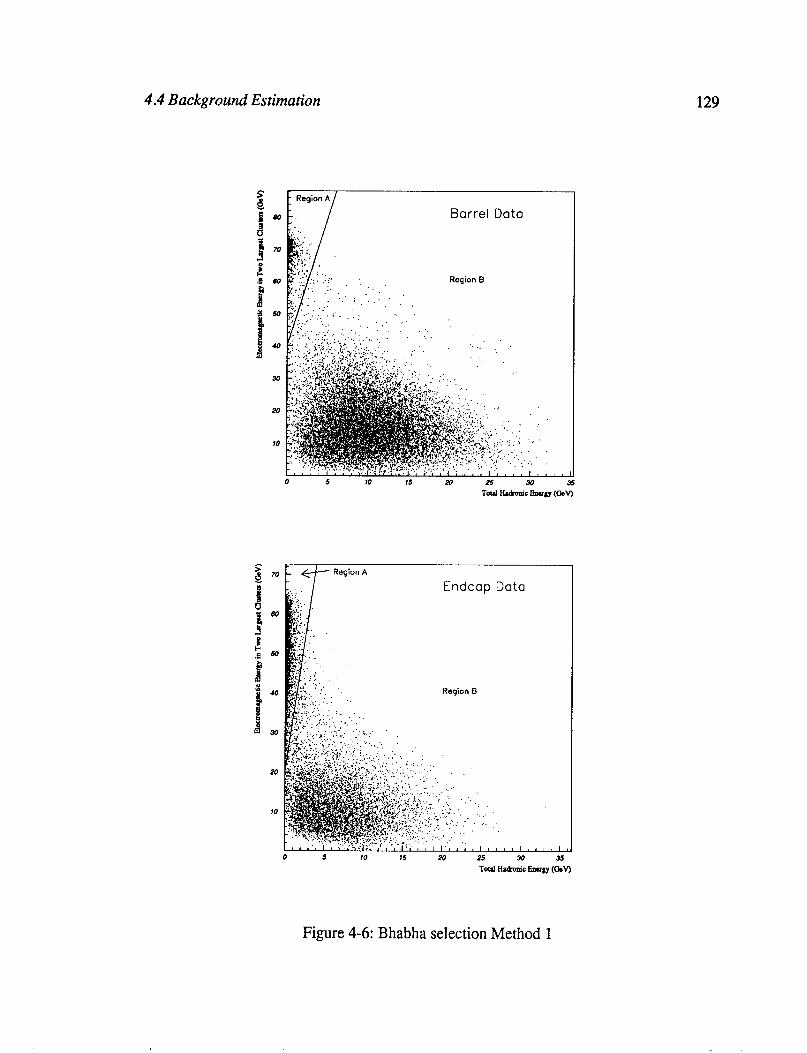
4.4 Background Estimation 129
F - Region A
i eo- _ _: Barrel Data
Region B
: . . : .;
:.
- 5 I5 .?5 30 .%
Total Hdronic Enqy (CJev)
Region A
Endcap Data
Region El
0 5 10 IS 20 25 30 3.5 TotdHdmicEnw#(ChV)
Figure 4-6: Bhabha selection Method 1
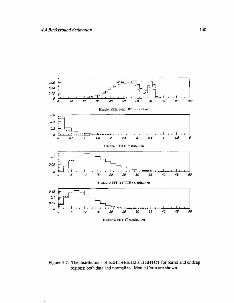
4.4 Background Estimation 130
0.06
,llIII,II III, II,, 0 10 20 30 40 50 60 70 80 90 100
Bhabha EEHII +EEHI2 distribution
0.6 ____
0.4 -
“~~~LLJ”“““““““““““” 0 0.5 1 1.5 2 2.5 3 3.5 4 4.5 5
0.1
0.05
0
Bhabha EHTOT distribution
0 5 10 75 20 25 30 35 40 45 50
Hadronic EEHIl+EEHI:! distribution
0 5 10 15 20 25 30 35 40 45 50
Hadronic EHTOT distribution
Figure 4-7: The distributions of EEHIl+EEHI2 and EHTOT for barrel and endcap regions; both data and normalized Monte Carlo are shown.
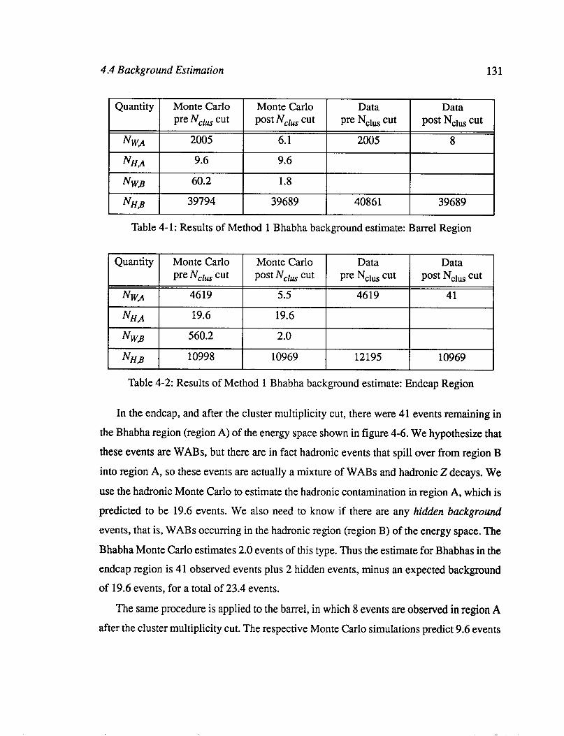
4.4 Background Estimation 131
Quantity
NWA
NHP
NW
NHS
Monte Carlo pre Ncrus cut
2005
9.6
60.2
39794
Monte Carlo post Ncrur cut
6.1
9.6
1.8
39689
Data Pre Nclus cut
2005
40861
Data post NclUS cut
8
39689
Table 4-l: Results of Method 1 Bhabha background estimate: Barrel Region
Quantity
NW
NHP
NW8
NH8
Monte Carlo pre Ncrus cut
4619
19.6
560.2
10998
Monte Carlo post Nclus cut
5.5
19.6
2.0
10969
Data Pre Nclus cut
4619
12195
Data post NclUS cut
41
10969
Table 4-2: Results of Method 1 Bhabha background estimate: Endcap Region
In the endcap, and after the cluster multiplicity cut, there were 41 events remaining in
the Bhabha region (region A) of the energy space shown in figure 4-6. We hypothesize that
these events are WABs, but there are in fact hadronic events that spill over from region B
into region A, so these events are actually a mixture of WABs and hadronic Z decays. We
use the hadronic Monte Carlo to estimate the hadronic contamination in region A, which is
predicted to be 19.6 events. We also need to know if there are any hidden background
events, that is, WABs occurring in the hadronic region (region B) of the energy space. The
Bhabha Monte Carlo estimates 2.0 events of this type. Thus the estimate for Bhabhas in the
endcap region is 41 observed events plus 2 hidden events, minus an expected background
of 19.6 events, for a total of 23.4 events.
The same procedure is applied to the barrel, in which 8 events are observed in region A
after the cluster multiplicity cut. The respective Monte Carlo simulations predict 9.6 events

4.4 Background Estimation 132
as hadronic contamination in region A, and 1.8 events as the hidden wide-angle Bhabha
background in region B.
We are interested in an upper bound on the Bhabha contamination from these predic-
tions. To summarize:
Barrel: 8 observed + 1.8 hidden, background of 9.6: 7.45 events at 95% c.1.
Endcap: 41 observed + 2.0 hidden, background of 19.6: 35.85 events at 95% c.1.
Total WAB background = (7.45+35.85)/(49392) = 0.000854
Which is to say, the total background fraction due to wide-angle Bhabhas,fbw, is less than
0.09% at the 95% confidence level. This result can also be expressed in terms of a central
value symmetrized about the 16.6% and 83.3% confidence contours:
NY = 27.Ok8.8
fP = (0.053 zk 0.017) % (4.5)
A major drawback in this method is the reliance on the Monte Carlo prediction of the
hidden backgrounds; that is, those Bhabhas that remain in the hadronic region (region B)
after the cluster multiplicity cut. Specifically, the Bhabha cluster multiplicity is underesti-
mated by the Monte Carlo, which means that the hidden background Nws is likely to be
underestimated in the barrel region. Additionally, the Bhabha Monte Carlo does not repro-
duce certain types of observed events wherein a Bhabha slips through a crack and deposits
significant energy in the hadronic section of the calorimeter, which again implies an under-
estimate of the hidden background.
Method
An alternative technique for extracting the WAB background was independently devel-
oped from that described above. The approach, however, is essentially the same: Develop
criteria to further isolate the WAB background within the A,Q sample in such a way that
fbw can be reliably estimated.
The quantity used here to perform the additional separation is the ratio R of the energy
in all LAC electromagnetic clusters (EETOT) to the total LAC cluster energy (ETOT). Fig-

4.4 Background Estimation 133
ure 4-8 (A) shows the distribution of R for the data (Pass One plus the energy and
imbalance cuts). The Bhabhas are clustered tightly about R = 1, but there is not very good
separation between the WABs and the hadronic events. We therefore invent a new ratio Rl,
which is the sum of all electromagnetic energy in clusters with greater than I GeV total
energy, divided by the total energy in the event. Figure 4-8 (B) gives the distribution of Rl
for the data. We see that the WAB-hadron separation with this modified electromagnetic
ratio is greatly improved. This is because hadronic events include of a relatively large num-
ber of low-energy electromagnetic clusters compared to WABs.
Using the 1 GeV cluster threshold, we may also define a new cluster multiplicity,
N clur,l, which is always less than or equal to N,l,. Figure 4-8 (C) shows the distribution of
N clus,l for the data (that is, for Pass One events that pass the energy and imbalance cuts, but
fail the cluster multiplicity cuts) as a solid histogram, and the Bhabha Monte Carlo overlaid
as a dotted histogram. The agreement is so good that the Monte Carlo is barely visible. This
is consistent with the hypothesis that the problem with modelling Nclus arises in the low
energy fragmentation in the Monte Carlo. In any case both data and Monte Carlo suggest
that more than 99% of all WABs have N,~,J less than 6. Figure 4-8 (D) shows the data
with the Pass Two energy and imbalance cuts, plus an Nclus,l < 6 cut, from which a WAB
threshold cut of Rl > 0.86 is derived. Figure 4-8 (E) shows the Rl distribution for Pass Two
events with Nclus,l less than 6, with the backgrounds selected for Rl > 0.86. Thus in the
Pass Two data sample, 0.34% (172 / 50707) of the events are found by the Method 2
Bhabha selection. It is clear from 4-8 (E) that not all selected events are WABs, so the
remaining question is what fraction of the 0.34% is due to non-WABs. Both tau and hadron
events are expected to contribute at a low level.
Based on or = 1.41 nb, we expect about 2550 tau events produced in the 1993 run. With
the 1 GeV cluster threshold cut discussed above, tau Monte Carlo predicts 61 tau events
which are mis-identified as WABs. This corresponds to 0.12% of the Am sample. Subtract-
ing this from above givesfbW = (0.22 + 0.05)%
To get an idea of how many hadron events are mis-identified as WABs, tracking infor-
mation is examined where available. The events selected by Method 2 as WAB candidates
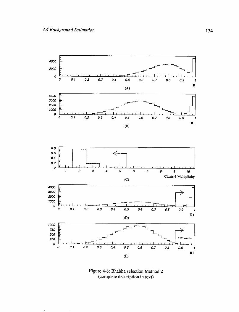
4.4 Background Estimation 134
0 0.1 0.2 0.3 0.4 0.5 0.6 0.7 0.8 0.9 1 R
(4
““““‘:” 0 0.1 0.2 0.3 0.4 0.5 0.6 0.7 0.8 0.9 1
Rl (B>
0.8 0.6 0.4 0.2
0 I , I , , , , , I , I , , , ,I(( ,(
1 2 3 4 5 6 7 8 9 10
cc> Cluster1 Multiplicity
i-l 4000 3000 2000 1000 - 0 1-1 I, I,,, I,,, ,,,,I,,
0 0.1 0.2 0.3 0.4 0.5 0.6 0.7 0.8 0.9 1
1000 750 500 250 172 events
0 0 0.1 0.2 0.3 0.4 0.5 0.6 0.7 0.8 0.9 1
Rl
Figure 4-8: Bhabha selection Method 2 (complete description in text)
4.4 Background Estimation 135
were examined for their CDC tracking content. 58% of the events did have CDC informa-
tion. Gf these events, the majority, 63%, have more that 6 good tracks, and hence are
primarily hadronic events. That is to say, that at least 36% of the estimate are definitely not
Bhabhas. Because of the uncertainty in extrapolating the track multiplicity analysis to those
events without CDC information, we cannot make a quantitative estimate of the hadronic
contamination in the endcap region. Therefore we subtract only those events positively
identified as hadronic decays in the barrel region, for a final Method 2 estimate of
f; = (0.14k 0.05) % (4.6)
This estimate represents an upper limit for the WAB contamination in the A, sample.
Result
It is not straightforward to reconcile the results of these two different Bhabha back-
ground estimates. Method 1 is probably an underestimate, due to its dependence on the
poorly modelled cluster multiplicities needed to determine the hidden backgrounds.
Method 2 on the other hand, is an overestimate, in that its selected background is certainly
contaminated by real hadronic events. The final background fraction is taken to be the aver-
age between theses two:
W fb = (0.10 + 0.06) % (4.7)
with a systematic uncertainty inflated to account to some degree for the discrepancy
between the two methods.
4.4.2 Cosmic Rays
It is possible for cosmic rays to deposit more than 20 GeV in the LAC. The dominant
mechanism is through the radiation of a hard photon by a cosmic muon. The effects of other
types of cosmic ray particles (electrons, neutrons, protons) is approximately two orders of
magnitude smaller than this muon contribution [63]. The total number of muons with
energy 2 20 GeV that cross the interaction point during the 1993 run is estimated to be
8400, based on the size of the interaction point, the total live-time of the SLD detector, and
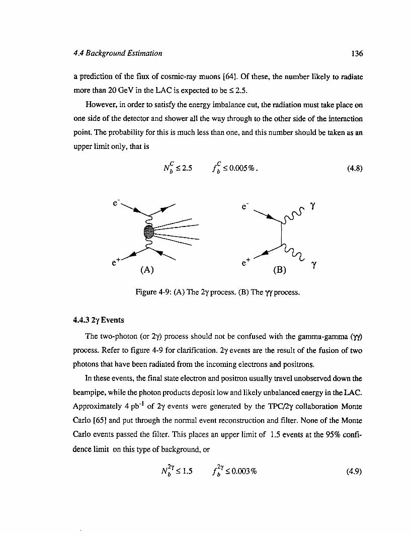
4.4 Background Estimation 136
a prediction of the flux of cosmic-ray muons [64]. Of these, the number likely to radiate
more than 20 GeV in the LAC is expected to be 52.5.
However, in order to satisfy the energy imbalance cut, the radiation must take place on
one side of the detector and shower all the way through to the other side of the interaction
point. The probability for this is much less than one, and this number should be taken as an
upper limit only, that is
NE I 2.5 f; I 0.005%. (4.8)
e-
x
Y
e+ w y
Figure 4-9: (A) The 2y process. (B) The “iy process.
4.4.3 2y Events
The two-photon (or 27) process should not be confused with the gamma-gamma (yy)
process. Refer to figure 4-9 for clarification. 2y events are the result of the fusion of two
photons that have been radiated from the incoming electrons and positrons.
In these events, the final state electron and positron usually travel unobserved down the
beampipe, while the photon products deposit low and likely unbalanced energy in the LAC.
Approximately 4 pb-’ of 2y events were generated by the TFW2y collaboration Monte
Carlo [65] and put through the normal event reconstruction and filter. None of the Monte
Carlo events passed the filter. This places an upper limit of 1.5 events at the 95% confi-
dence limit on this type of background, or
NfY I 1.5 f? IO.o03% w-9
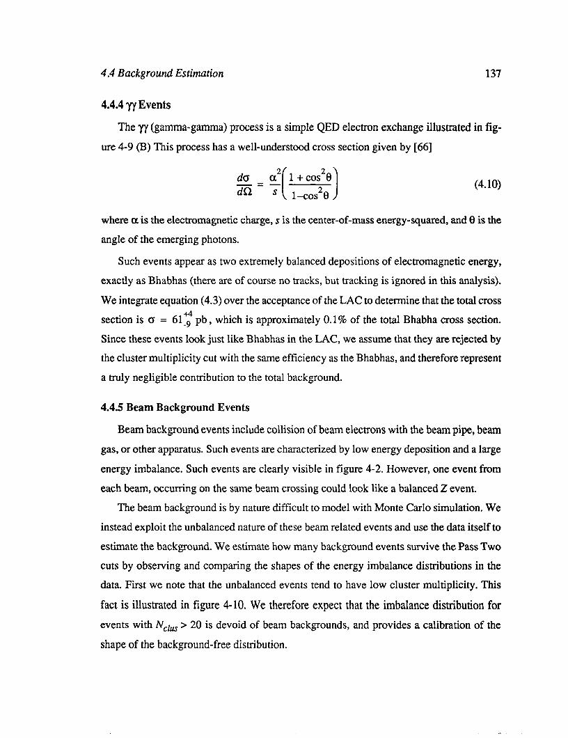
4.4 Background Estimation 137
4.4.4 yy Events
The yy (gamma-gamma) process is a simple QED electron exchange illustrated in fig-
ure 4-9 (B) This process has a well-understood cross section given by [66]
-=- (4.10)
where a is the electromagnetic charge, s is the center-of-mass energy-squared, and 8 is the
angle of the emerging photons.
Such events appear as two extremely balanced depositions of electromagnetic energy,
exactly as Bhabhas (there are of course no tracks, but tracking is ignored in this analysis).
We integrate equation (4.3) over the acceptance of the LAC to determine that the total cross
section is 0 = 61: pb , which is approximately 0.1% of the total Bhabha cross section.
Since these events look just like Bhabhas in the LAC, we assume that they are rejected by
the cluster multiplicity cut with the same efficiency as the Bhabhas, and therefore represent
a truly negligible contribution to the total background.
4.4.5 Beam Background Events
Beam background events include collision of beam electrons with the beam pipe, beam
gas, or other apparatus. Such events are characterized by low energy deposition and a large
energy imbalance. Such events are clearly visible in figure 4-2. However, one event from
each beam, occurring on the same beam crossing could look like a balanced 2 event.
The beam background is by nature difficult to model with Monte Carlo simulation. We
instead exploit the unbalanced nature of these beam related events and use the data itself to
estimate the background. We estimate how many background events survive the Pass Two
cuts by observing and comparing the shapes of the energy imbalance distributions in the
data. First we note that the unbalanced events tend to have low cluster multiplicity. This
fact is illustrated in figure 4-10. We therefore expect that the imbalance distribution for
events with Nclus > 20 is devoid of beam backgrounds, and provides a calibration of the
shape of the background-free distribution.
4.4 Background Estimation 138
0.6
0.4
0.2
: .j,: : :_:..
-11111111 0 IO 20 30 40 50 60 70
cluncr MultiplbAy
Figure 4- 10: The Pass One data in I versus NClus variable space.
Figures 4-l l(A) and 4- 11 (B) show the normalized imbalance distributions for data with
21 I NCrU < 25 and 12 5 NClus I 20, respectively.
Assuming the background is primarily in the region 0.4 <I < 0.6, then the expected sig-
nal fraction is estimated from figure 4-l l(B) by the ratio of the number of events in the 0.4
< I c 0.6 range (Nb,r) to the number of events in the I < 0.4 range (N&. Let N,,r and NS2
be the numbers in the corresponding ranges in figure 4-l l(A). The estimated number of
backgrounds and resulting background fraction vb’) is now
N: = Na ,-N , (4.11)
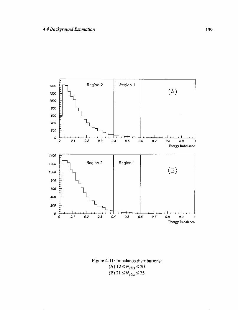
4.4 Background Estimation 139
I-
1400
1200
1000
800
600 P
Region 2 Region 1
(A)
0 0.1 0.2 0.3 0.4 0.5 0.6 0.7 0.8 0.9 1 Energy Imbalance
7200
1000
800
600
400
200
0
Region 1
(B)
7 , , , , , , , , , ! . ! ! , I I , , , I , , , ,111
0 0.1 0.2 0.3 0.4 0.5 0.6 0.7 0.8 0.9 1 EnergyImbalance
Figure 4- 11: Imbalance distributions: (A) 12 I NClus I20 (B)21 IN,,525
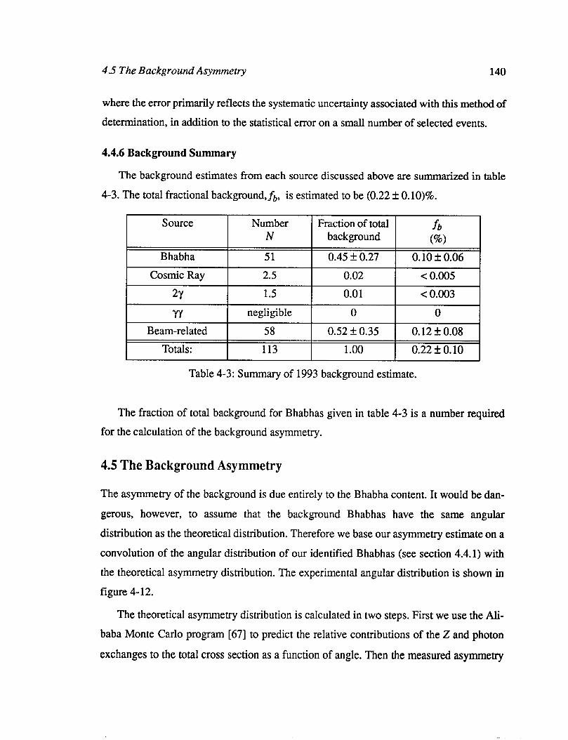
4.5 The Background Asymmetry 140
where the error primarily reflects the systematic uncertainty associated with this method of
determination, in addition to the statistical error on a small number of selected events.
4.4.6 Background Summary
The background estimates from each source discussed above are summarized in table
4-3. The total fractional background,fb, is estimated to be (0.22 f O.lO)%.
Source
Bhabha
Cosmic Ray
2Y
Number N
51
2.5
1.5
Fraction of total background
0.45 f 0.27
0.02
0.01
n negligible 0
Beam-related 58 0.52 zk 0.35
Totals: 113 1.00
fb (%o)
0.10 f 0.06
< 0.005
< 0.003
0
0.12+0.08
0.22 Tk 0.10
Table 4-3: Summary of 1993 background estimate.
The fraction of total background for Bhabhas given in table 4-3 is a number required
for the calculation of the background asymmetry.
4.5 The Background Asymmetry
The asymmetry of the background is due entirely to the Bhabha content. It would be dan-
gerous, however, to assume that the background Bhabhas have the same angular
distribution as the theoretical distribution. Therefore we base our asymmetry estimate on a
convolution of the angular distribution of our identified Bhabhas (see section 4.4.1) with
the theoretical asymmetry distribution. The experimental angular distribution is shown in
figure 4- 12.
The theoretical asymmetry distribution is calculated in two steps. First we use the Ali-
baba Monte Carlo program [67] to predict the relative contributions of the 2 and photon
exchanges to the total cross section as a function of angle. Then the measured asymmetry
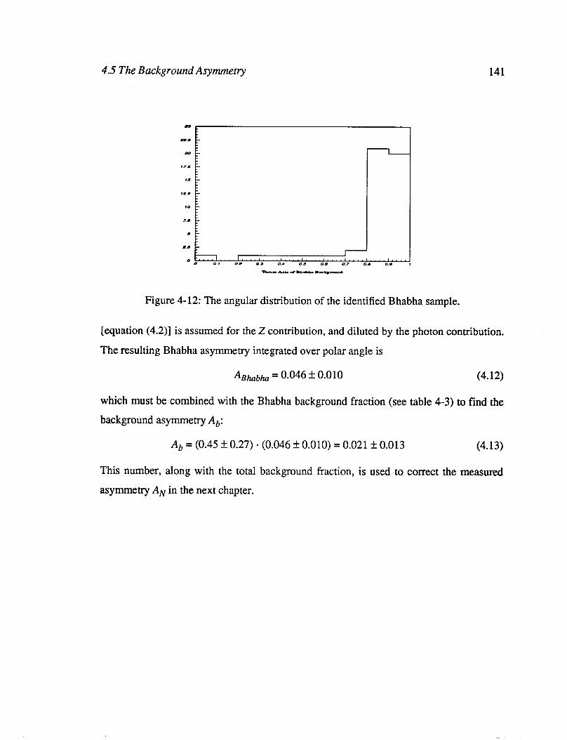
4.5 The Background Asymmetry 141
Figure 4- 12: The angular distribution of the identified Bhabha sample.
[equation (4.2)] is assumed for the 2 contribution, and diluted by the photon contribution.
The resulting Bhabha asymmetry integrated over polar angle is
A &&ha = 0.046 Z!I 0.010 (4.12)
which must be combined with the Bhabha background fraction (see table 4-3) to find the
background asymmetry Ab:
A, = (0.45 rt 0.27) - (0.046 +O.OlO) = 0.021 k 0.013 (4.13)
This number, along with the total background fraction, is used to correct the measured
asymmetry A, in the next chapter.

Chapter 5
Analysis and Results
It was shown in Chapter 1 how the measured asymmetry AN is related to Am. It was
assumed that there no other asymmetries that might contaminate the measurement. An
additional implicit assumption was that the average Compton measured asymmetry, (Pz) ,
is equal to the true luminosity-weighted polarization at the SLC interaction point, ( Pe) . In turns out that in 1993 this may not have been the case. Both of these assumptions will be
addressed in this chapter, and some systematic cross-checks which have been made over
the last two years will also be discussed, after which the final result will be presented.
5.1 The Chromaticity Effect
Because the SLC was run in flat-beam mode, with very small vertical emittance, the verti-
cal size of the beam at the lP may have been limited by 3rd order chromatic aberrations.
This is to say, that the focussing may have been energy-dependent. As a result, the lumi-
nosity may also have been energy dependent. As discussed in section 2.2, the spin
orientation is certainly energy dependent. Therefore there could be a luminosity-polariza-
tion correlation where the lower energy tail of the beam has lower polarization and also
does not contribute significantly toward the creation of Zs. This implies that the instanta-
142
5.1 The Chromatic@ Effect 143
neous polarization at the SLC interaction point, P,, would be a weighted-average
number density and luminosity
over
re =
I
(5.1) N(E)L(E)dE
where N is the number density of electrons, P is the polarization, and L the luminosity, all
functions of the energy E.
At the Compton polarimeter interaction point, on the other hand, the electron beam has
zero nominal dispersion. Also, the Compton target laser spot is large compared to the elec-
tron beam, and as a result the polarimeter measures the polarization of the entire beam
profile:
pc = ~N(W’(W e
f N(E)dE (5.2)
Therefore there can be a difference between (Pz) and (P,) that should be taken into
account, a difference encompassed in the parameter 5, which we call the chromaticity
correction.
(P,) = (1 + 5) u(f) (5.3)
Although the chromaticity effect may vary over time during the run, only the average lumi-
nosity-weighted polarization is important to the analysis, and thus a single correction
parameter is sufficient.
5.1.1 The Chromaticity Model
The various inputs necessary to calculate 5 are shown in figure 5-1. The first is the
intensity (N) versus energy profile, which is measured by wire scans. The second is the
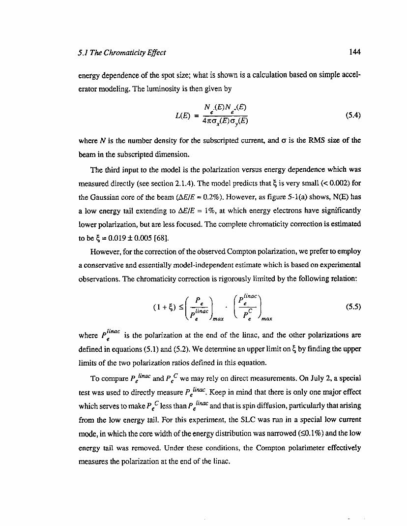
5.1 The Chromaticity EfSect 144
energy dependence of the spot size; what is shown is a calculation based on simple accel- erator modeling. The luminosity is then given by
L(E) = Ne-(E)Ne+(E) 4~o,(E)o,(E) (5.4)
where N is the number density for the subscripted current, and CT is the RMS size of the
beam in the subscripted dimension.
The third input to the model is the polarization versus energy dependence which was
measured directly (see section 2.1.4). The model predicts that 5 is very small (< 0.002) for
the Gaussian core of the beam (AE/E = 0.2%). However, as figure 5-l(a) shows, N(E) has
a low energy tail extending to AE/E = l%, at which energy electrons have significantly
lower polarization, but are less focused. The complete chromaticity correction is estimated
to be 5 = 0.019 f 0.005 [68].
However, for the correction of the observed Compton polarization, we prefer to employ a conservative and essentially model-independent estimate which is based on experimental
observations. The chromaticity correction is rigorously limited by the following relation:
(5.5)
linac where P, is the polarization at the end of the linac, and the other polarizations are
defined in equations (5.1) and (5.2). We determine an upper limit on 5 by finding the upper
limits of the two polarization ratios defined in this equation.
To compare Pelinnc and Pet we may rely on direct measurements. On July 2, a special
test was used to directly measure P, l iMC Keep in mind that there is only one major effect .
which serves to make P,’ less than Pelinac and that is spin diffusion, particularly that arising
from the low energy tail. For this experiment, the SLC was run in a special low current
mode, in which the core width of the energy distribution was narrowed (SO. 1%) and the low
energy tail was removed. Under these conditions, the Compton polarimeter effectively
measures the polarization at the end of the linac.
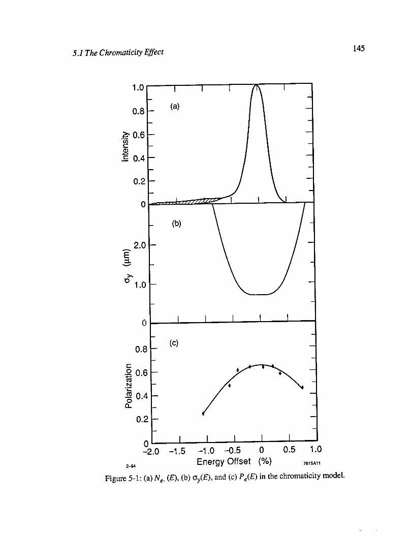
5.1 The Chromatic@ EfSect
0.8
0.8 _ w
.z 0.6 5 ‘C 52 0.4 -
g
0 .2 -
C .O -1.5 -1 .o -0.5 0 0.5 1.0
244 Energy Offset (Oh) 7615All
Figure 5-l: (a) N,- (E), (b) o,(E), and (c) P,(E) in the chromaticity model.
145
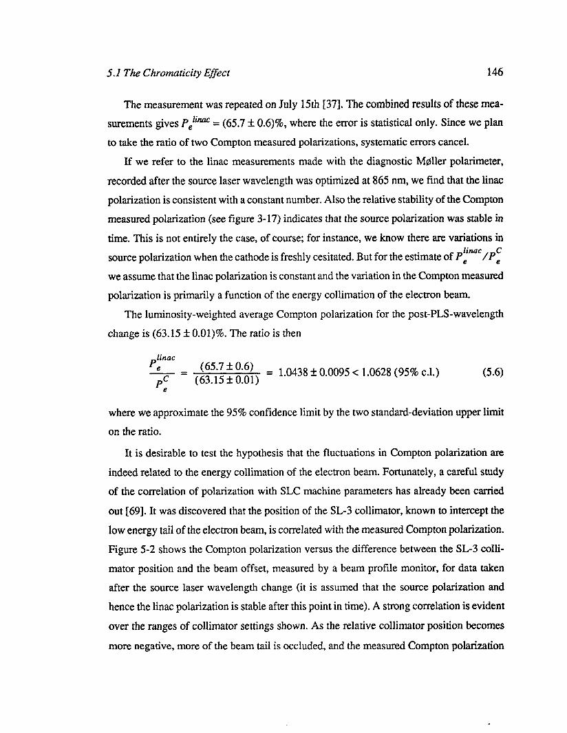
5.1 The Chromatic@ Effect 146
The measurement was repeated on July 15th [37]. The combined results of these mea-
surements gives P,lim = (65.7 + 0.6)%, where the error is statistical only. Since we plan
to take the ratio of two Compton measured polarizations, systematic errors cancel.
If we refer to the linac measurements made with the diagnostic Moller polarimeter,
recorded after the source laser wavelength was optimized at 865 nm, we find that the linac
polarization is consistent with a constant number. Also the relative stability of the Compton
measured polarization (see figure 3-17) indicates that the source polarization was stable in
time. This is not entirely the case, of course; for instance, we know there are variations in
source polarization when the cathode is freshly cesitated. But for the estimate of Pff’““/PF
we assume that the linac polarization is constant and the variation in the Compton measured polarization is primarily a function of the energy collimation of the electron beam.
The luminosity-weighted average Compton polarization for the post-PLS-wavelength
change is (63.15 _+ O.Ol)%. The ratio is then
linac ‘e (65.7 f 0.6) =
p: (63.15 Z!Z 0.01) = 1.0438 +, 0.0095 < 1.0628 (95% c.1.) (5.6)
where we approximate the 95% confidence limit by the two standard-deviation upper limit
on the ratio.
It is desirable to test the hypothesis that the fluctuations in Compton polarization are
indeed related to the energy collimation of the electron beam. Fortunately, a careful study
of the correlation of polarization with SLC machine parameters has already been carried
out [69]. It was discovered that the position of the SL-3 collimator, known to intercept the
low energy tail of the electron beam, is correlated with the measured Compton polarization.
Figure 5-2 shows the Compton polarization versus the difference between the SL3 colli-
mator position and the beam offset, measured by a beam profile monitor, for data taken
after the source laser wavelength change (it is assumed that the source polarization and
hence the linac polarization is stable after this point in time). A strong correlation is evident
over the ranges of collimator settings shown. As the relative collimator position becomes
more negative, more of the beam tail is occluded, and the measured Compton polarization
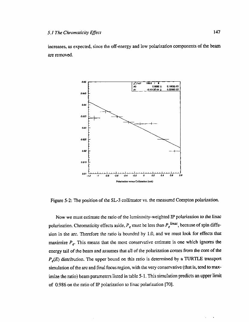
5.1 The Chromatic@ Efiect 147
increases, as expected, since the off-energy and low polarization components of the beam
are removed.
0.66
0.615
X)/“df 133.6 I 6 A0 0.6262 f 0.1603E-03 Al -0.1013E41f 0.3206603
Figure 5-2: The position of the SL-3 collimator vs. the measured Compton polarization.
Now we must estimate the ratio of the luminosity-weighted IP polarization to the linac
polarization. Chromaticity effects aside, P, must be less than Pefim, because of spin diffu-
sion in the arc. Therefore the ratio is bounded by 1.0, and we must look for effects that
maximize P,. This means that the most conservative estimate is one which ignores the
energy tail of the beam and assumes that all of the polarization comes from the core of the
P,(E) distribution. The upper bound on this ratio is determined by a TURTLE transport
simulation of the arc and final focus region, with the very conservative (that is, tend to max-
imize the ratio) beam parameters listed in table 5- 1. This simulation predicts an upper limit of 0.986 on the ratio of IP polarization to linac polarization [70].

5.1 The Chromatic@ EfSect 148
1 Parameter 1 Assumed Limit 1
I 5 I > 650 l.trn+rad I
> 100 pm-prad
I OE I > 0.15%
I
P,/PyaC < 0.986
Table 5-1: Parameters of beam transport simulation.
The final limit on the chromaticity corrections is
1 I ( 1 + 5) I ( 1.0628.0.986) or
O<cSO.O48 (5.7)
We take the central value of the allowed range as the correction, and the 62.8% width of
the allowed range as the error (since the correction has a more or less equal probability of
lying anywhere in the allowed range) to find
5 = 0.024+ 0.016. (5.8)
Figure 5-3 shows the predictions of the full accelerator model developed by F. Decker
[68]. In this figure, all polarizations are scaled to P, liMC The ratio of the solid line to the .
dashed line (for a given year) is equal to (I+-\). It was decided by the collaboration not to
use this model as the correction because many inputs remain untested by data. The point of
interest is that, in 1994, the chromaticity effect should be negligible, for two reasons. First,
an upgrade of the final focus optics will reduce the chromatic aberrations. And second, the
so-called “over-compression” technique will be used in the damping ring to remove the
low-energy tail of the electron bunch (the amount of energy-tail is represented by the
degree to which the dotted lines deviate from 100%).

5.2 Additional Corrections to AL& 149
90
f 5
5 5
*. f
- -== Polarization at SLC IP ‘***..
: : : :
t
I__ Polarization at Compton IP k.. i ::t::~:: Beam Intensity -.
s
-2.0 -1.6 -1.2 -0.8 -0.4 0 2-94 Energy Cut (%) 7615AlO
Figure 5-3: Predictions of the chromaticity model.
5.2 Additional Corrections to ALL
The following equation shows the first order effect of various asymmetries on A,:
A LR = .fb (AN - AJ - AL - AiAp
_ E o’(Ecm) -A, -A, +
cm Wcm> (P,)Pp 1
(5.9)
In this equation, AN is the measured asymmetry defined in equation (1.29), (P,) is the
luminosity-weighted average polarization defined in equation (1.30)& is the background
fraction in the sample, and Ab is the asymmetry of that background, as discussed in section
4.5. The polarization asymmetry, Ap, is directly measured by the polarimeter, as discussed
in section 3.3.1. Other terms in equation (5.9) include the luminosity asymmetry (AL), the
center-of-mass energy (Ecm) and the energy asymmetry (AE), the cross section (0) and the derivative of the cross section (6) at the center-of-mass energy, the efficiency asymmetry
(AJ, and the positron polarization (Pp), which are discussed in the sub-sections below.

5.2 Additional Corrections to ALR 150
52.1 Luminosity Asymmetry (AL)
It has been shown empirically that the current extracted from strained cathodes varies with the orientation of linearly polarized light with respect to the strain axis. Therefore
residual linear polarization in the source laser could result in an asymmetry in the extracted
electron current, which in turn leads to a net left-right luminosity asymmetry Ab This lumi-
nosity asymmetry is estimated through the 120 Hz data of beam current toroids and
radiative Bhabha monitors located in the North Final Focus region. We find the asymmetry
to be AL = (3.8 + 5.0)x10m5 which leads to a correction of (-0.037 + 0.049)% to ALR [71].
The beam current asymmetry and AQ of all other quantities correlated with it were reduced by once reversing the sign of the field in the LTR solenoid. By changing the sign
of the field in the LTR solenoid, electrons that were previously stored with spins up in the
damping ring are now stored down. Those same electrons now have the opposite helicity
at the IP. In other words, the meaning of the source helicity bits has changed, and the sign
of any source-related asymmetry also changes.
A cross check on the luminosity asymmetry is performed by examining a sample of
125,375 small-angle Bhabha events measured by the LUM system. The observed left-right
counting asymmetry, AN, for small angle Bhabha events is very small (= -1.5x10A.P, for
the LUM acceptance), and therefore this quantity is a direct measure of AL. The measured
VidUeOfANLuM= (-32 f 28)x10A is consistent with the more precisely determined value of
the luminosity asymmetry.
5.2.2 Energy Asymmetry (AE)
In equation (5.9), (3 and CT’ are the cross section and derivative of the cross section with
respect to energy, respectively, evaluated at the average operating energy. The energy
asymmetry is measured directly by the energy spectrometer (see section 2.4) 120 Hz data
to be (4.4 f 0.1)x 10e7. This asymmetry follows the beam current asymmetry due to beam
loading in the accelerator. At the measured value of 91.26 GeV the fractional derivative of
the cross section with respect to energy is not terribly steep (0.023 GeV-‘). Thus the fiat-
tional correction to ALR of (0.00090 + 0.00002)% is negligible.

5.2 Additional Corrections to ALR 151
5.2.3 Efficiency Asymmetry (A&
The detector itself could induce an false asymmetry by preferentially accepting Zs with one handedness. The only difference between left-handed and right-handed Zs is that the
polar-angular distribution of outgoing fermions is reversed, or, to put it another way, the
distribution of fermions for a left-handed event is the same as the distribution of anti-fer-
mions in a right-handed events. Therefore the only way to have a non-zero A, is if fermions
and anti-fermions are not accepted equally in the calorimeter.
First of all, it is assumed that the process of calorimetry itself is symmetric with respect
to matter and anti-matter. Given this assumption, it is sufficient to have either an azimuth-
ally symmetric magnetic field or uniform detection efficiency for a given polar angle in order for the determination of Am to be independent of efficiency effects. In the case of the
SLD, both of these conditions are true: The LAC is highly uniform and symmetric (both in 8 and Q) in its construction, and the SLD solenoidal field implies magnetic azimuthal
symmetry.
Even without the assumption of matter/anti-matter detection efficiency, it is sufficient
that the efficiency be polar-angle symmetric, that is, that E(q,6) = E(q,n-e), which is also a
symmetry of the SLD construction. Even if there were some non-uniformity in the calorim-
eter energy response, beyond the symmetries already described, our energy cut-off is so
low (see figure 4-4) that such a bias would have a negligible effect. For all of these reasons,
the A, correction term is assumed to be negligible.
5.2.4 Positron Polarization (Pp)
It has already been discussed in section 2.1.1 that any residual polarization of positrons
is correlated with the scavenger electron polarization and has no effect on Am. Therefore,
in order for there to be an effect, the positrons must have some fixed-sign polarization
building up somewhere. The only known mechanism for the build-up of fixed-sign positron
polarization is the Sokolov-Turnov effect: the induced quantum spin-flip transitions in the
magnetic field of the positron damping ring.
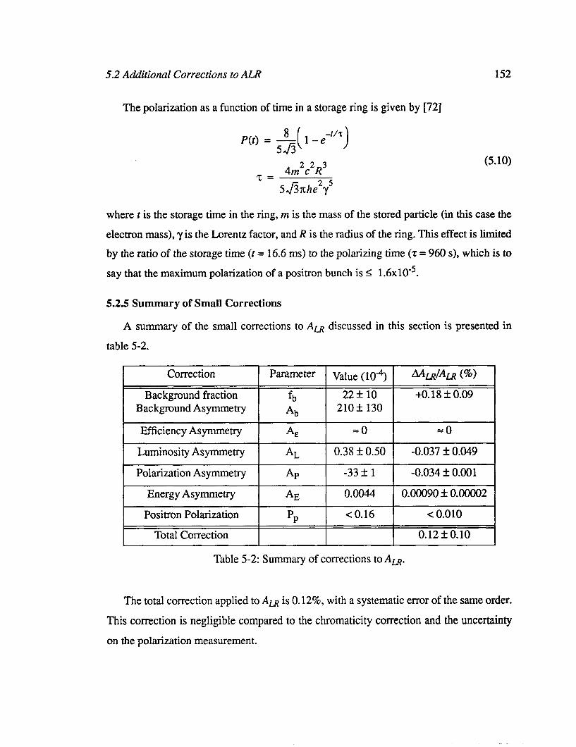
5.2 Additional Corrections to ALR 152
The polarization as a function of time in a storage ring is given by [72]
P(t) = -$[ 1 -e-l”)
z = 4m2c2R3
5+f3xhe2y5
(5.10)
where t is the storage time in the ring, m is the mass of the stored particle (in this case the
electron mass), y is the Lorentz factor, and R is the radius of the ring. This effect is limited
by the ratio of the storage time (t = 16.6 ms) to the polarizing time (z = 960 s), which is to
say that the maximum polarization of a positron bunch is I 1.6~10~~.
5.2.5 Summary of Small Corrections
A summary of the small corrections to A,Q discussed in this section is presented in
table 5-2.
Correction
Background fraction Background Asymmetry
Efficiency Asymmetry
I Luminosity Asymmetry
1 Positron Polarization
I Total Correction
AL I 0.38 f 0.50
I PI3 I < 0.16
AA&Am (%) 1 +O. 18 f 0.09
Table 5-2: Summary of corrections to Am.
The total correction applied to A,TJ is 0.12%, with a systematic error of the same order.
This correction is negligible compared to the chromaticity correction and the uncertainty
on the polarization measurement.

5.3 Systematic Cross-checks 153
5.3 Systematic Cross-checks
In addition to the systematic effects discussed above, there are several “non-effects” to be considered, that is, effects that could conceivably affect the measurement but have been shown not to do so.
5.3.1 Fixed Polarizer Test
The cross-checks discussed in this section and the section following were motivated by
the one-time discrepancy between the Linac Moller Polarimeter and Compton polarization
measurements, which was on the order of 10%. Thus these checks were designed to look
for a large systematic error of essentially unknown origin, unlike the precision checks on polarimetry discussed in Chapter 3.
It is possible that the circular polarization delivered by the CLS transport line is less
than the reported 99%, that somehow the Pockels cell scans are only finding a local maxi- mum rather than the absolute maximum circular polarization. In order to discount this
possibility, a special test (called the “fixed polarizer test”) was prepared [73].
In this test, the circularly polarizing Pockels cells were removed, and linearly polarized
light was transmitted to the SLC vacuum entrance window. At this point a quarter wave
plate was introduced, and the circular polarization of the beam immediately before the
entrance window was measured to be 0.995 f 0.005. Then nominal beam polarization mea-
surements were made (with fixed photon helicity), and the results of those measurements
are shown in figure 5-4.
The average beam polarization measured before the quarter-wave plate was installed was 0.607 f 0.004. The average beam polarization measured after the quarter-wave plate
was installed was 0.601+ 0.005. Thus the Pockels cell polarization technique is eliminated
as a possible source of large unknown systematic error.
5.3.2 Current Asymmetry Test
Having eliminated the target polarization as a source of large unknown systematic
error, the only remaining possibility was in the measurement of the experimental asymme-
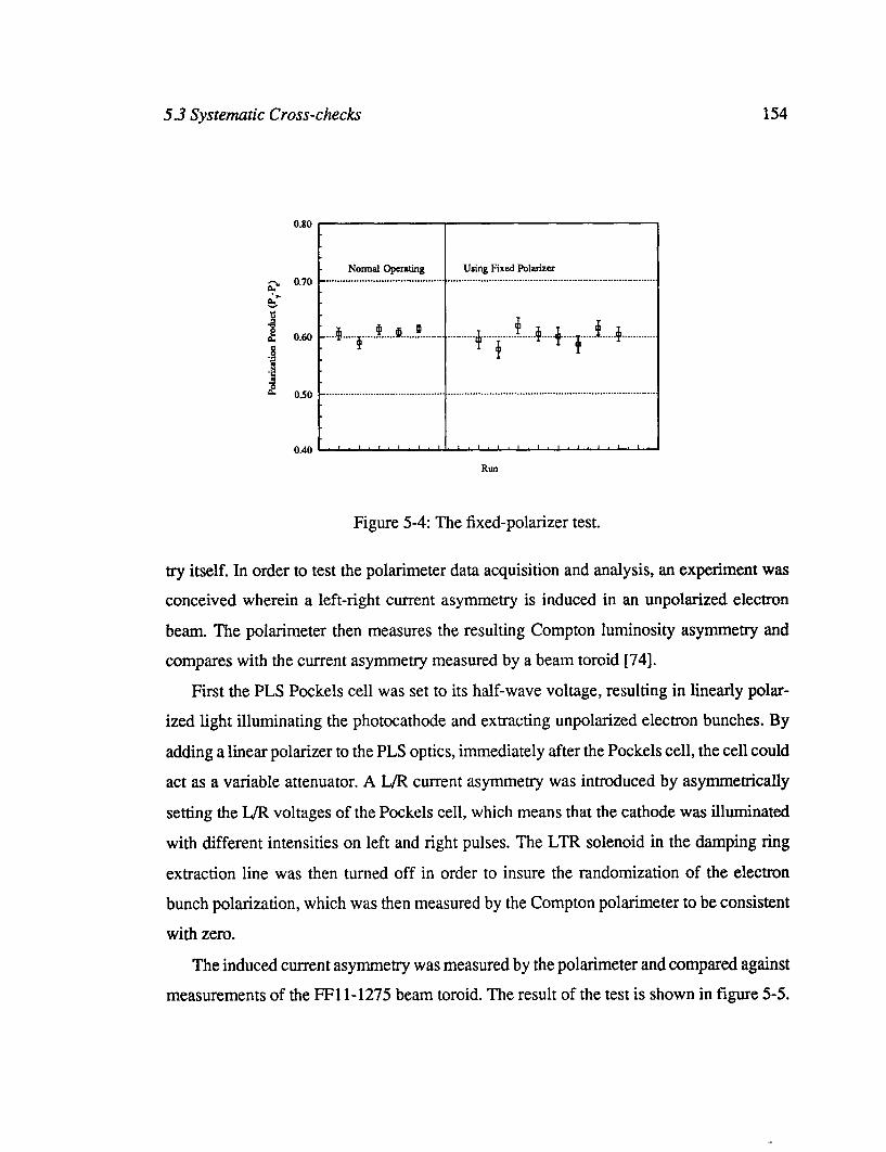
5.3 Systematic Cross-checks 154
0.80
Nomd Operating Using Fixed Polarizer 0.70 _................._......................... ,....._.......__.............................................................
Figure 5-4: The fixed-polarizer test.
try itself. In order to test the polarimeter data acquisition and analysis, an experiment was conceived wherein a left-right current asymmetry is induced in an unpolarized electron
beam. The polarimeter then measures the resulting Compton luminosity asymmetry and compares with the current asymmetry measured by a beam toroid [74].
First the PLS Pockels cell was set to its half-wave voltage, resulting in linearly polar-
ized light illuminating the photocathode and extracting unpolarized electron bunches. By
adding a linear polarizer to the PLS optics, immediately after the Pockels cell, the cell could
act as a variable attenuator. A L/R current asymmetry was introduced by asymmetrically
setting the L/R voltages of the Pockels cell, which means that the cathode was illuminated
with different intensities on left and right pulses. The LTR solenoid in the damping ring
extraction line was then turned off in order to insure the randomization of the electron
bunch polarization, which was then measured by the Compton polarimeter to be consistent
with zero.
The induced current asymmetry was measured by the polarimeter and compared against
measurements of the FFl l-1275 beam toroid. The result of the test is shown in figure 5-5.
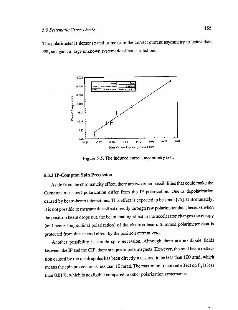
5.3 Systematic Cross-checks 155
The polarimeter is demonstrated to measure the correct current asymmetry to better than
3%, so again, a large unknown systematic effect is ruled out.
f -0.24 . . ’ . . ’ ’ . . ’ ’ .
-0.26 -0.22 -0.18 -0.14 -0.10 -0.06 -0.02 0.02
Man Curmtt Asymmetry. Tomid 1275
Figure 5-5: The induced current asymmetry test.
5.3.3 IP-Compton Spin Precession
Aside from the chromaticity effect, there are two other possibilities that could make the Compton measured polarization differ from the IP polarization. One is depolarization
caused by beam-beam interactions. This effect is expected to be small [75]. Unfortunately,
it is not possible to measure this effect directly through raw polarimeter data, because when
the positron beam drops out, the beam loading effect in the accelerator changes the energy
(and hence longitudinal polarization) of the electron beam. Summed polarimeter data is
protected from this second effect by the positron current veto.
Another possibility is simple spin-precession. Although there are no dipole fields
between the IP and the CIP, there are quadrupole magnets. However, the total beam deflec-
tion caused by the quadrupoles has been directly measured to be less than 100 prad, which means the spin precession is less than 10 mrad. The maximum fractional effect on P, is less
than O.Ol%, which is negligible compared to other polarization systematics.
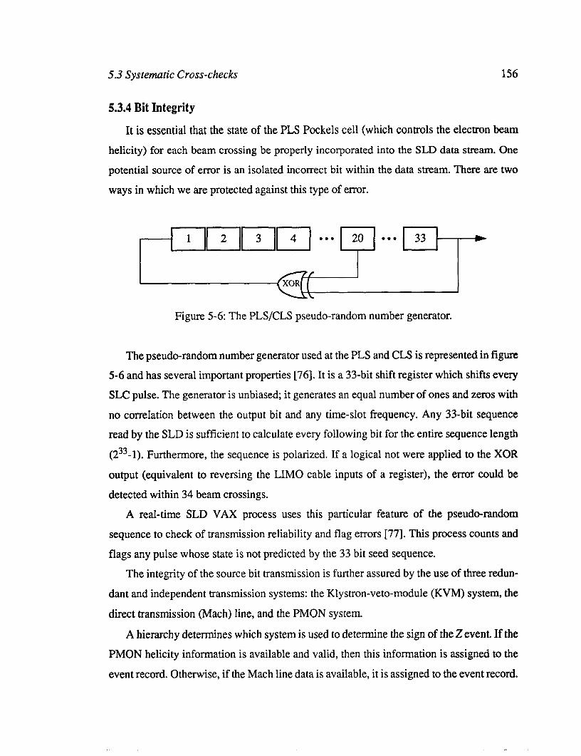
5.3 Systematic Cross-checks 156
5.3.4 Bit Integrity
It is essential that the state of the PLS Pockels cell (which controls the electron beam
helicity) for each beam crossing be properly incorporated into the SLD data stream. One
potential source of error is an isolated incorrect bit within the data stream. There are two
ways in which we are protected against this type of error.
Figure 5-6: The PLSKLS pseudo-random number generator.
The pseudo-random number generator used at the PLS and CLS is represented in figure
5-6 and has several important properties [76]. It is a 33-bit shift register which shifts every
SLC pulse. The generator is unbiased; it generates an equal number of ones and zeros with
no correlation between the output bit and any time-slot frequency. Any 33-bit sequence
read by the SLD is sufficient to calculate every following bit for the entire sequence length
(233-l). Furthermore, the sequence is polarized. If a logical not were applied to the XOR
output (equivalent to reversing the LIMO cable inputs of a register), the error could be
detected within 34 beam crossings.
A real-time SLD VAX process uses this particular feature of the pseudo-random
sequence to check of transmission reliability and flag errors [77]. This process counts and
flags any pulse whose state is not predicted by the 33 bit seed sequence.
The integrity of the source bit transmission is further assured by the use of three redun-
dant and independent transmission systems: the Klystron-veto-module (KVM) system, the
direct transmission (Mach) line, and the PMON system.
A hierarchy determines which system is used to determine the sign of the 2 event. If the
PMON helicity information is available and valid, then this information is assigned to the
event record. Otherwise, if the Mach line data is available, it is assigned to the event record.
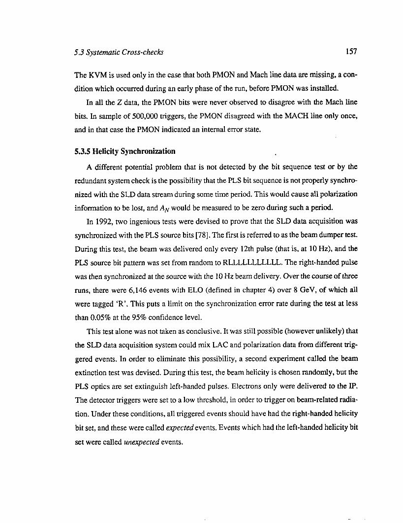
5.3 Systematic Cross-checks 157
The KVM is used only in the case that both PMON and Mach line data are missing, a con-
dition which occurred during an early phase of the run, before PMON was installed.
In all the Z data, the PMON bits were never observed to disagree with the Mach line
bits. In sample of 500,000 triggers, the PMON disagreed with the MACH line only once,
and in that case the PMON indicated an internal error state.
5.3.5 Helicity Synchronization
A different potential problem that is not detected by the bit sequence test or by the redundant system check is the possibility that the PLS bit sequence is not properly synchro-
nized with the SLD data stream during some time period. This would cause all polarization
information to be lost, and AN would be measured to be zero during such a period.
In 1992, two ingenious tests were devised to prove that the SLD data acquisition was
synchronized with the PLS source bits [78]. The first is referred to as the beam dumper test.
During this test, the beam was delivered only every 12th pulse (that is, at 10 Hz), and the
PLS source bit pattern was set from random to RLLLLLLLLLLL. The right-handed pulse
was then synchronized at the source with the 10 Hz beam delivery. Over the course of three
runs, there were 6,146 events with EL0 (defined in chapter 4) over 8 GeV, of which all
were tagged ‘R’, This puts a limit on the synchronization error rate during the test at less
than 0.05% at the 95% confidence level.
This test alone was not taken as conclusive. It was still possible (however unlikely) that
the SLD data acquisition system could mix LAC and polarization data from different trig-
gered events. In order to eliminate this possibility, a second experiment called the beam
extinction test was devised. During this test, the beam helicity is chosen randomly, but the
PLS optics are set extinguish left-handed pulses. Electrons only were delivered to the IP.
The detector triggers were set to a low threshold, in order to trigger on beam-related radia-
tion. Under these conditions, all triggered events should have had the right-handed helicity
bit set, and these were called expected events. Events which had the left-handed helicity bit
set were called unexpected events.

5.3 Systematic Cross-checks 158
The combined results of the beam extinction tests showed 5896 expected events with 9
unexpected events, which gives a conservative error rate of (0.16 + 0.06)%, or less than
0.3% at the 95% confidence level. We call this conservative because it is probably a gross
over-estimate: the unexpected events are almost certainly due to noise in the LAC firing the
trigger and not an actual error in helicity assignment.
In early 1993 the beam extinction test was repeated and again confirmed that the SLD
data acquisition was properly synchronized with the PLS helicity information.
5.3.6 Cut Bias
It would be alarming if the value of the measured asymmetry were somehow a function of the variables with which we select the data. Figure 5-7 shows the measured asymmetry
in bins of the Pass Two cut variables. The solid line shows the value of AN on each graph.
There are clearly no significant statistical anomalies in the energy and energy imbalance
distributions.
At first sight, there appears to be a significant deviation of AN in the smallest bin of clus-
ter multiplicity. We have carefully studied events in this bin. A hand scan of all events
reveals nothing unusual in the event topologies. One might postulate that this bin could
have a large number of Bhabhas that have just missed being removed by the multiplicity
cut. However, the angular distribution of the events shows that they are mostly in the barrel
region, the region in which Bhabhas do not have a significantly degraded asymmetry. Other
beam backgrounds with null asymmetries are also unlikely to be concentrated in the barrel
region. We are therefore forced to conclude that there is no excessive contamination in this
particular Nclus bin, and the observed deviation of AN is a two-sigma statistical fluctuation.
It is worthwhile to note that AN is also unbiased by the cut on the time difference
between the Z event and the polarization measurement. It can be further shown that, to the
extent that the polarimeter randomIy samples the true beam poIarization, far fewer mea-
surements than are made are actually necessary. This is again a direct consequence of the
dependence of Am on the average rather than the instantaneous polarization. Nevertheless,
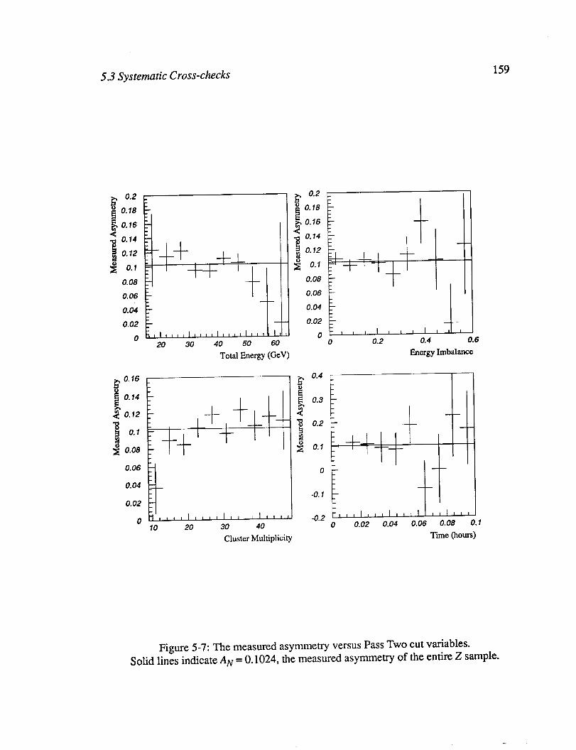
5.3 Systematic Cross-checks 159
B 0.2
a B 0.78 0.16 4 1 0.74
1 0.12
3 0.1 0.08
0.06
0.04
0.02
0
B 0.16
i 0.14
$ 0.12
;B 3 0.1 3 E 0.08
0.06
0.04
0.08
0.06
0.04
0.02
2 0 20 30 40 50 60
Total Energy (GeV)
---t . I I '
t L ' 1.
% 0.2
e, “E 0.18 0 0.76 4 1 0.14
3 0.72
2 0.1
i Oe4 1 0.3 3 0.2
5 2 0.7
0
-0.1
-0.2
Energy Imbalance
0 0.02 0.04 0.06 0.08 0.7
Cluster Multiplicity Tie (hours)
Figure 5-7: The measured asymmetry versus Pass Two cut variables. Solid lines indicate AN = 0.1024, the measured asymmetry of the entire Z sample.
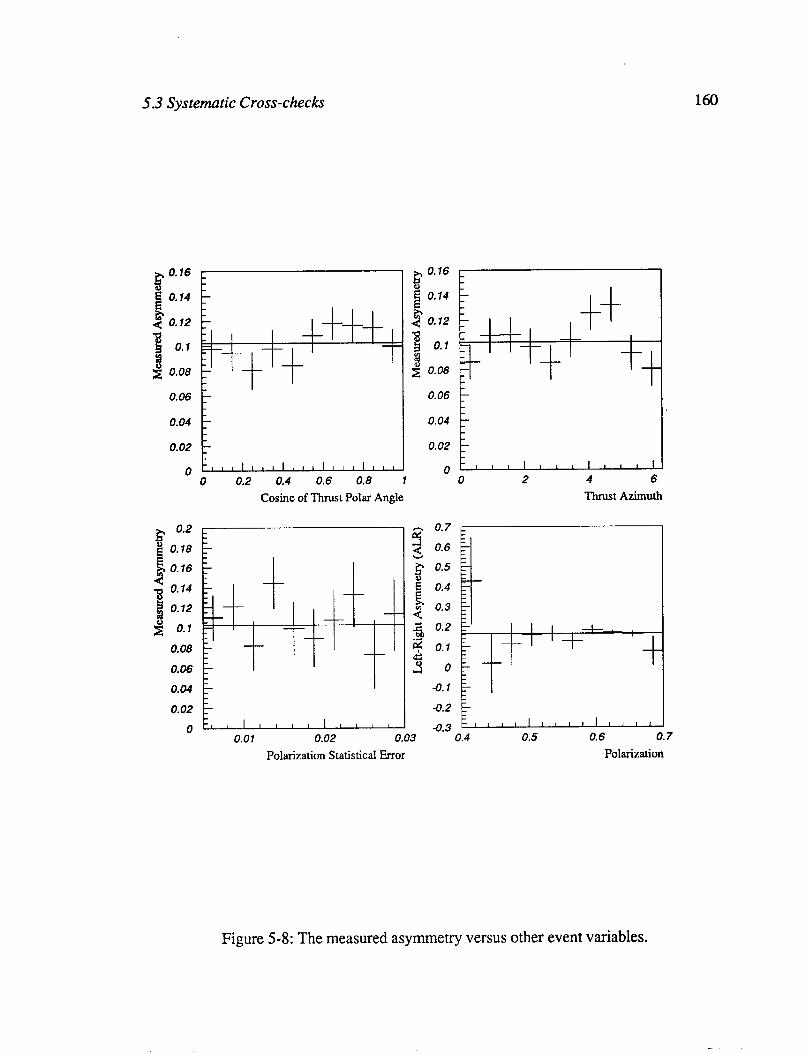
5.3 Systematic Cross-checks 160
B 0.16 _ B 0.16 _
B 0.14 r i 0.14 1
4 0.12 r --ttt- 4 0.12 r t+ 3
+ B 0.1 b E-
E 0.08 F --t +
g 0.1 L
2 0.08 = --t 0.06 0.06 r
0.04 - 0.04 r
0.02 - 0.02 -
0 lll’lll’ill’lll’lll 0 I I 1 I I I I I I I I 0 0.2 0.4 0.6 0.8 1 0 2 4 6
Cosine of Thrust Polar Angle Thrust Azimuth
I; 0.2
QJ
E 2
0.18 0.16
1 0.14
3 3 0.12
x 0.1
0.08
0.06
2 0.7
a_ 0.6
3 0.2
q 0.1
4 0
-0.1 0.04
0.02 olL-kd-d :~~Lllllllllllll . 0.01 0.02 0.03 0.4 0.5 0.6 0.7
Polarization Statistical Error Polarization
I I --I-. .
‘$
Figure 5-8: The measured asymmetry versus other event variables.

5.3 Systematic Cross-checks 161
in the unlikely case that the polarization did vary wildly during polarimeter down time, it remains safe to employ the time cut.
Figure 5-8 shows the measured asymmetry in bins of some other quantities of interest.
The co& and Q distributions indicate no unusual geometrical acceptance effects. There is no apparent correlation between AN and polarization error, which could appear if some
background contamination were correlated with polarimeter noise and thus poltimeter sta-
tistical error. The value of Am in polarization bins (that is, the measured asymmetry for
events in the given range of polarization divided by the average polarization in that range)
is also seen to be consistent with the average value for the run (the chromaticity correction
has not been applied to the data shown).
5.3.7 Total Systematic Uncertainty
Table 5-3 shows the sum of all systematic uncertainties. Our total systematic error is
2.1%. For the 1994 run, the chromaticity effect will be gone and the polarimeter error will
be less than or equal to l%, so we expect our total systematic error will be 1% or less.
Asymmetry Corrections
Total Systematic Uncertainty
Table 5-3: Total systematic uncertainty on the ALL measurement.

5.4 Results and Comparisons 162
5.4 Results and Comparisons
We have now compiled sufficient information to extract Am from the data. We will com-
pare the result of this measurement with other electroweak measurements and the Standard
Model. It is important to note, however, that Am on its own makes no prediction about the
Standard Model; only a comparison of at least two independent measurements can do so.
5.4.1 Extracting ALR
From the results cited in chapter 4, we find the measured asymmetry, AN:
A, = WL - NJ (NL + NR>
= (27225 -22167) = 0 1024 + 0 0045 (27225 +22167) ’ - * (5.11)
where the error quoted is purely statistical.
From the results cited in Chapter 3, including the chromaticity correction derived in this
chapter, we find the average polarization:
= 0.634 k 0.013 (5.12)
where the error is purely systematic, a combination of the polarimeter systematic error and
the chromaticity error.
Inserting these results and those of table 5-3 into equation (5.9) we determine the fol-
lowing result for Am:
A,,(91.26 GeV) = 0.1617 + O.O071(stat.) f O.O033(syst.) (5.13)
5.4.2 Extracting the Weinberg angle from ALR
In order to compare to other electroweak experiments, we would like to convert our
energy-dependent value of AJJ into an observation of the effective Weinberg angle,
sin 2 eff 8, . We use the ZFITTER program [24] to model initial-state radiation, and to account
for the photon exchange and electroweak interference that occurs as a result of being off
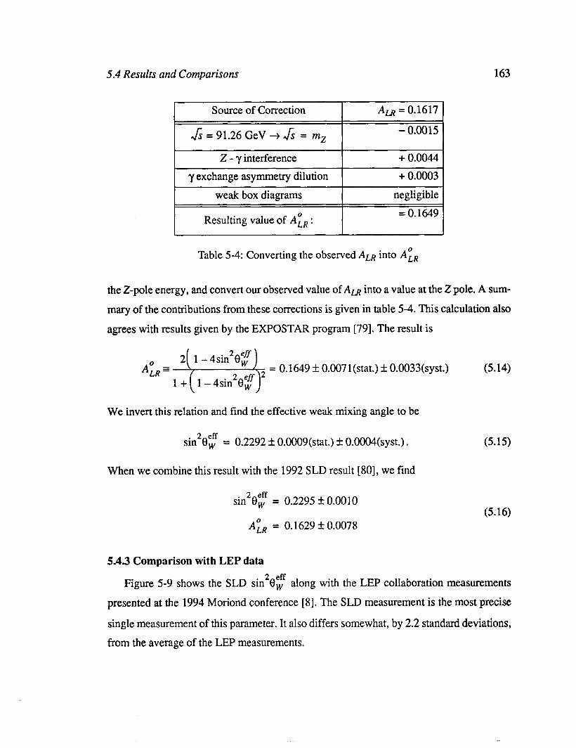
5.4 Results and Comparisons 163
Source of Correction
& = 91.26 GeV + $s = mz
ALR = 0.1617
- 0.0015
2 - y interference y exchange asymmetry dilution
+ 0.0044 + 0.0003
weak box diagrams
Resulting value of AIR :
negligible = 0.1649
Table 5-4: Converting the observed ALR into AIR
the Z-pole energy, and convert our observed value of Am into a value at the Z pole. A sum-
mary of the contributions from these corrections is given in table 5-4. This calculation also
agrees with results given by the EXPOSTAR program [79]. The result is
= 0.1649 k 0.007 1 (stat.) k O.O033(syst.) (5.14)
We invert this relation and find the effective weak mixing angle to be
2 eff sin 8, = 0.2292 + O.O009(stat.) + O.O004(syst.).
When we combine this result with the 1992 SLD result [SO], we find
sin 2 0, eff = 0.2295 k 0.0010
ALR = 0.1629 + 0.0078
(5.15)
(5.16)
5.4.3 Comparison with LEP data
Figure 5-9 shows the SLD sin2f$ along with the LEP collaboration measurements
presented at the 1994 Moriond conference [8]. The SLD measurement is the most precise
single measurement of this parameter. It also differs somewhat, by 2.2 standard deviations,
from the average of the LEP measurements.
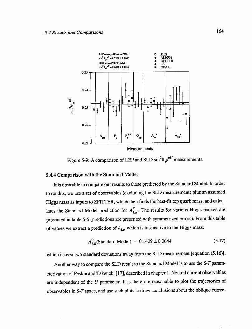
5.4 Results and Comparisons 164
UP Avaqa (Maid 94):
.i2Q* IO.2321 f oMM6
SlD Vdw (92+‘93 da: ,dQd L 0.2.m * o.cao
•I SLD l ALEPH A DELPHI 0 L3 m OPAL
A’ Pt ml
Measurements
i
AC PB
Figure 5-9: A comparison of LEP and SLD sin2eWeff measurements.
5.4.4 Comparison with the Standard Model
It is desirable to compare our results to those predicted by the Standard Model. In order
to do this, we use a set of observables (excluding the SLD measurement) plus an assumed
Higgs mass as inputs to ZFITIER, which then finds the best-fit top quark mass, and calcu-
lates the Standard Model prediction for ALR. The results for various Higgs masses are
presented in table 5-5 (predictions are presented with symmetrized errors). From this table
of values we extract a prediction of Am which is insensitive to the Higgs mass:
AL,(Standard Model) = 0.1409 + 0.0044 (5.17)
which is over two standard deviations away from the SLD measurement [equation (5.16)].
Another way to compare the SLD result to the Standard Model is to use the S-Tparam-
eterization of Peskin and Takeuchi [ 171, described in chapter 1. Neutral current observables are independent of the U parameter. It is therefore reasonable to plot the trajectories of
observables in S-T space, and use such plots to draw conclusions about the oblique correc-
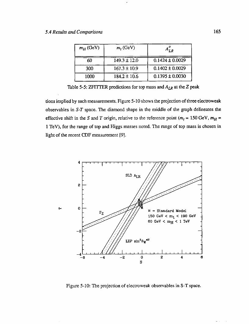
5.4 Results and Comparisons 165
mH GW
60 300 1000
m, (GW
149.3 I!z 12.0 167.3 f 10.9 184.2 It 10.6
AL?
0.1424 f 0.0029 0.1402 f 0.0029 0.1395 f 0.0030 1
Table 5-5: ZFITTER predictions for top mass and Am at the Z peak
tions implied by such measurements. Figure 5-10 shows the projection of three electroweak
observables in S-T space. The diamond shape in the middle of the graph delineates the
effective shift in the S and T origin, relative to the reference point (mt = 150 GeV, “ZH =
1 TeV), for the range of top and Higgs masses noted. The range of top mass is chosen in
light of the recent CDF measurement [9].
:’ . .
-2
-A r
Ki = Standard Model 150 GeV < mt < 190 GeV _ 60 GeV < mH < 1 TeV
1-6 -4 -2 0 2 4 6 S
Figure 5-10: The projection of electroweak observables in S-T space.

5.5 Future Experimental Precision 166
In this graph, the incompatibility of the SLD measurement with the LEP measurements
and the Standard Model is most obvious. It is interesting to note that if the SLD value of 2 eff sin 0, is correct, the measurement favors a region of negative S, which is theoretically
challenging to explain. That is, it is difficult to create models which predict negative values
of S. Supersymmetric and technicolor models, for instance, both predict positive S [ 171.
Figure 5- 11 shows the result of fitting the best values of S, T, and a, to 13 observables, including the SLD measurement of Am [81]. Again, the Standard Model is encompassed
by the parallelogram for the same range of top and Higgs masses given in figure 5-10. The
fit results are
S = - 0.35 If: 0.23 T= + 0.24 + 0.22
as = 0.124 2 0.005 (5.18)
X2/d.o.f. = 14.8/10, probability = 13.9%
The overall fit is consistent with the Standard Model, as a result of the statistical power
of the LEP measurements. However, we again see a slight but not terribly significant ten-
dency towards regions of negative S.
5.5 Future Experimental Precision
SLD has been approved for four more years of polarized running, and with even higher
electron polarization and increased luminosity, we hope to measure the effective Weinberg
angle to a precision of 0.0003. The projected error on sin 2 eff 0, for and 80% polarization
cathode and a systematic error of 1% is shown in figure 5-12. If the same central value of
Am reported in this document is measured in future running, the Standard Model will be in
trouble, and electroweak physics will become even more interesting than it already is.

5.5 Future Experimental Precision 167
mt = 190 GeV
0.75 - mH = 60 GeV
0.50 - 66% c.1.
90% c.1.
E 0.25 -
0.00 - 150 GeV 1000 GeV
-0.25 - 3% = Standard Model
r -0.50’““““““““““““““”
-2 -1.5 -1 -0.5 0 0.5 1 S
Figure 5-l 1: Standard Model fit to electroweak observables.
100000
Number of Zs
1000000
Figure 5-12: The projected error on the effective weak mixing angle.
References
[l] A concise description of the 1993 experiment is found in:
K. Abe et al., Phys. Rev. Lett. 73,25 (1994).
It must be noted that the analysis presented in this thesis differs in
some details from that described in the citation.
[2] S. L. Glashow, Nucl. Phys. 22,579 (1961).
[3] A. Salam and J. C. Ward, Phys. Lett. 13, 168 (1964);
A. Salam, Elementary Particle Theory: Relativistic Groups and Analytic@
(8th Nobel Symposium), edited by N. Svartholm (Almqvist and Wiskell,
Stockholm, 1968), p. 367.
[4] S. Weinberg, Phys. Rev. Lett. 19, 1264 (1967).
[5] We follow the notation and exposition of C. Quigg, Gauge Theories of Strong,
Weak, and Electromagnetic Interactions, The Benjamin/Cummings Publishing
Company, Inc., Reading, Massachusetts, 1983.
[6] P. W. Higgs, Phys. Rev. Lett. 12, 132 (1966); 13,508 (1964);
F? W. Higgs, Phys. Rev. 145, 1156 (1966);
F. Englert and R. Brout, Phys. Rev. Lett. 13,321 (1964);
G. S. Guralnik et al., Phys. Rev. Lett. 13,585 (1964);
T. W. B. Kibble, Phys. Rev. 155, 1554 (1967).
168

169
[7] Particle Data Group, Phys. Rev. D45,ll (1992), Part II.
[8] B. Pietrzyk, LAPP-EXP-94.07, May 1994.
Summary of LEP results presented at the 1994 Moriond conference.
[9] F. Abe et al., FERMILAB-PUB-94-097-E, April 1994.
[lo] A review of the properties of ALR can be found in:
D. C. Kennedy et al., Nucl. Phys. B321,83 (1989).
[ll] M. Swartz, SLAC-PUB-5219, March 1990.
[ 121 For an comprehensive discussion of the Z lineshape and initial-state radiation, see
M. E. Peskin, SLAC-PUB-5210, March 1990, and
Proceedings of the 17th SLAC Summer Institute on Particle Physics,
edited by E. C. Brennan, p. 71, (1990).
[ 131 E. A. Kuraev and V. S. Fadin, Sov. J. Nucl. Phys. 41,466 (1985).
[ 141 G. Bonneau and F. Martin, Nucl. Phys. B27,38 1 (197 1).
[15] R. Calm, Phys. Rev. D36,2666 (1987).
[16] W. Marciano, Phys. Rev. D20,274 (1979).
[17] M. E. Peskin and T. Takeuchi, Phys. Rev. D46,381 (1992).
[18] D. C. Kennedy and B. W. Lynn, Nucl. Phys. B322,l (1989).
[19] B. W. Lynn and C. Verzegnassi, Nuovo Cim. 94A, 15 (1986).
[20] A. Sirlin, Phys. Rev. D22,971 (1980).
[21] M. Demarteau et al., Combining W Mass Measurements, DONOTE 2115.
[22] B. Lynn, M. Peskin, and R. G. Stuart, Physics at LEP,
Proceedings of the Workshop, Geneva, Switzerland, edited by
J. Ellis and R. Peccei (CERN Report # CERN 86-02, Geneva, 1986), Vol. 1.

170
[23] M. Consoli and W. Hollik, Z Physics at LEP I, Proceedings of the Workshop, Geneva, Switzerland,
edited by G. Altarelli, R. Kleiss, and C. Verzegnassi
(CERN Report # CERN 89-08, Geneva, 1989), Vol. 1.
[24] D. Bardin et al., CERN-TH. 6443/92, May 1992. See also
D. Bardin et al., Z. Phys. C44,493 (1989).
[25] A. Olshevski, P N. Ratoff, and P B. Renton, CERN-PPE/93-88, May 1993.
[26] N. Phinney, Int. J. Mod. Phys. A, Proc. Suppl. 2A, 45 (1993).
[27] D. Schultz et al., SLAC-PUB-6275, June 1993.
[28] D. T. Pierce and F. Meier, Phys. Rev. B13,5484 (1976).
[29] L. G. Levchuk, KHFTI-92-32, June 1992.
[30] R. E. Kirby et al., SLAC-PUB-6006, December 1992.
[31] M. Woods et al., SLAC-PUB-5894, September 1992.
[32] C. Adolphson, F.-J. Decker, and J. Seeman, Flat Beam Studies in the SLC Linac,
Proceedings of the 1993 Part. Act. Conf., Washington, D.C., 1993.
1331 C. Adolphson et al., SLAC-PUB-6118, May 1993.
[34] K. Pitts, Ph.D. Thesis, University of Oregon, SLAC Report 446, 1994.
[35] J. D. Jackson, Classical Electrodynamics, 2nd ed.,
J. Wiley and Sons Inc., New York, 1975, p. 558.
[36] T. Limberg, P. E mma, and R. Rossmanith, SLAC-PUB-6210, May 1993.
[37] F.-J. Decker et al., SLD Note #238, January 1994.
It must be explained that at the time this document was released, the final Compton
polarimeter calibration was not yet available. All numbers in this thesis have been
corrected for the final calibration, and differ slightly from those in the Note cited.
171
[38] M. Swartz et al., SLAC-PUB-6467, June 1993.
Contains a complete treatment of SLAC Moller polarimetry.
[39] R. Elia, Ph.D. Thesis, Stanford University, SLAC Report 429, 1994.
[40] J. Kent et al., SLAC-PUB-4922, March 1989.
[41] G. Blaylock, SLD Physics Note #22, June 1993, and private communication.
[42] The SLD Design Report, SLAC Report 273, 1984.
[43] C. J. S. Damerell et al., Nucl. Inst. and Meth. A328,472 (1987).
[44] S. C. Berridge et al., IEEE Trans. Nucl. Sci. NS-39,242 (1992).
[45] K. Abe et al., SLAC-PUB-6226, June 1993.
[46] P N. Burrows et al., SLAC-PUB-5305, August 1990. See also
A. C. Benvenuti et al., SLAC-PUB-5332, November 1990;
D. C. Williams, Ph.D. Thesis, Massachusetts Institute of Technology,
SLAC Report 445,1994.
[47] D. Axen et al., Nucl. Inst. Meth. A328,472 (1993).
[48] M. Swartz, SLAC-PUB-4656, June 1988, and
Proceedings of the 15th SLAC Summer Institute on Particle Physics,
edited by E. C. Brennan, p. 83, (1988).
[49] H. Veltman, Phys. Rev. D40,2810 (1989).
[50] B. Schumm and R. Elia, SLD Note #222, November 1992.
[51] B. Schumm, R. King, and E. Torrence, SLD Note #241, March 1994.
[52] S. D. Drell, SLD Note #226, September 1992.
[53] A. Lath and M. Woods, SLD Note #236, June 1994.
[54] I? C. Rowson, M. Fero, M. Woods, and M. Zolotorev,
SLD Note #216 (revised), October 1992.
172
[55] M. Woods, SLD Note #223, October 1992.
[56] J. M. Yamartino, SLD Physics Note #14, November 1992.
[57] S. Gonzalez, SLD Physics Note #24, October 1993.
[58] J. M. Yamartino, Ph.D. Thesis, Massachusetts Institute of Technology,
SLAC Report 426,1994. See Appendix A.
[59] K. T. Pitts, SLD Physics Note #20, April 1993.
[60] H. Park et al., SLD Physics Note #19, March 1993.
[61] R. Ben-David and H. Park, SLD Physics Note #18, July 1993.
[62] R. Frey et al., SLD Note #243, in progress.
[63] J. F. Ziegler, Nucl. Inst. and Meth. 191,419 (1981).
[64] R. K. Adair and H. Kasha, “Cosmic-Ray Muons,” Muon Physics,
Volume 1: Electromagnetic Interactions, edited by V. W. Hughes and C. S. Wu,
Academic Press (1977).
[65] H. Aihara et al., Z. Phys. C34, 1 (1987).
[66] F. E. Low, Phys. Rev. Lett., 14,238 (1965).
[67] W. Beenakker, F. A. Berends, and S. C. van der Marck,
Nucl. Phys. B349,323 (1991).
[68] F. J. Decker, Luminosity Weighted Polarization Corrections, CN-399, 1994.
[69] B. Schumm, SLD Note #234, October 1993.
[70] B. Schumm et al., SLD Note #240, March 1994, and
Paul Emma, private communication.
[7 l] l? Rowson, SLD Note #244, in progress.
[72] A. A. Sokolov and I. M. Turnov, Dokl. Akad. Nauk. SSSR. 153, 1052 (1963).

173
[73] M. Fero and D. Calloway, SLD Note #233, August 1993.
[74] M. Fero et al., SLD Note #232, August 1993.
[75] K. Yokoya and P Chen, SLAC-PUB-4692, September 1988.
[76] T. Junk and T. Johnson, SLD Note #227, November 1992.
[77] Tom Junk, private communication.
[78] P C. Rowson, et al., SLD Note #219, September 1992,
and Peter Rowson, private communication.
[79] D. C. Kennedy et al., Z. Phys. C53,617 (1992).
[80] K. Abe et al., Phys. Rev. Lett. 70,2515 (1993).
The result reported in this citation:
2 eff sin 8, = 0.2378 zb 0.0056 (stat.) + 0.0005 (syst.)
[8 l] The following measurements are included in the Standard Model fit:
% had, Fz, R,, AjTmns, AiTarks, A;rarks, QFB, A, and A, (from P,) [8];
mW [211, QW [82], R, [83], ALR [this document].
[82] M. C. Noecker et al., Phys. Rev. Lett. 61,310 (1988); [experiment]
S. A. Blundell et al., Phys. Rev. Lett. 65, 1411 (1990). [theory]
[83] G. Altarelli et al., CERN-TH. 6770/93.