Policy Note

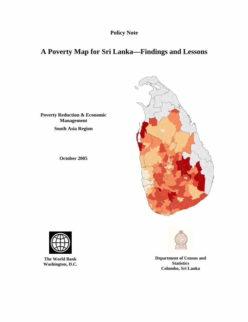
A Poverty Map for Sri Lanka—Findings and Lessons

Poverty Reduction & Economic

Management

South Asia Region

October 2005

The World Bank Washington, D.C.

Department of Census and

Statistics Colombo, Sri Lanka

A Poverty Map for Sri Lanka—Findings and Lessons This policy note summarizes results and experience of a poverty mapping exercise in Sri Lanka that has been conducted in close collaboration with the Department of Census and Statistics (DCS) since 2003—we gratefully acknowledge the overall support of Mr. Nanayakkara (Director General, DCS) and the technical support from Mr. Tilakaratne (Deputy Director, Sample Surveys Division, DCS) and Dr. Satharasinghe (Deputy Director, Cartography and Mapping Division, DCS).∗ The Sri Lanka Poverty Mapping exercise is an outcome of an ongoing poverty monitoring technical assistance (TA) for DCS. Besides poverty mapping, there have been other areas of work under this TA—this includes assistance to develop a consensus on the official poverty line for Sri Lanka, planned workshops to disseminate the poverty line and the poverty map, and ongoing support for the potential expansion of the HIES to include indicators to monitor social sector outcomes. Technical support for the poverty mapping exercise is now complete, which includes capacity building and training to improve data entry/processing facility and create a laboratory for Geographical Information System in DCS. In July 2005, the DCS and the Bank jointly organized a workshop to disseminate the official poverty line and the results of the poverty mapping exercise in Colombo. The Bank will continue to support the DCS in a broad dissemination of the poverty map.

Poverty Mapping is a useful method to uncover spatial heterogeneity in poverty incidence that is prominent in Sri Lanka. This note provides maps of poverty estimates at subnational levels and links them with maps of remoteness and drought. This note should be printed in color for visual clarity.

The results of the poverty mapping exercise are presented in Section 2. The poverty maps at the Divisional Secretary’s (DS) division level show (i) DS divisions with severe deprivation are more common in the southernmost areas of the country; but pockets of high poverty exist in even relatively better off districts such as Colombo; (ii) large numbers of poor people are found not only in Central province and the southern part of the Badulla district, but also in Western Province; (iii) the comparison between accessibility to towns and markets and poverty headcount ratios shows clearly that poverty in Sri Lanka is closely associated with geographical isolation.

The poverty maps have had impact even as they were being developed. For example, interim poverty maps (at the DS division level) could be overlaid against GIS maps of tsunami-affected areas to indicate the overlap between poverty and extent of tsunami damage. Recently, GoSL has also found it useful to compare DS division level poverty estimates with the extent of Samurdhi coverage in these divisions, to get a rough idea of the extent of mis-targeting. This in turn has helped generate a consensus around the need for better targeting.

A series of dissemination workshops for poverty maps are planned in the next fiscal year to create a network of long-term users of poverty maps and inform them of proper uses of such maps. Poverty maps can be easily misused due to its visual and intuitive appeal. This makes it all the more important to stress the limitations and caveats on the use of poverty maps. Such maps should be used only as the indicative first step for designing and planning poverty programs, and are not substitutes for actual targeting, particularly at the household level.

The umbrella task—Poverty Monitoring TA for Sri Lanka—is task managed by Tara Vishwanath, with a team comprising of Yoko Kijima, Peter Lanjouw, Ambar Narayan, Kinnon Scott, and Nobuo Yoshida. Nobuo Yoshida provided the technical support and capacity building to the DCS staff for the Poverty Mapping exercise. Peter Lanjouw provided expert advice for the exercise, particularly in its early stages. Uwe Deichmann and Piet Buys helped in translating the poverty estimates into visual maps, and guided the DCS team in creating a new laboratory of Geographical Information System. Ambar Narayan has assisted this exercise by providing useful inputs throughout the project. Yoko Kijima contributed to setting up the official poverty line, which is used for the poverty mapping exercise. Tomoyuki Sho contributed to the simulations conducted in section 4. ∗ We also appreciate and acknowledge support from many others in DCS, especially, Mrs. Vidyaratne, Mr. Fernando, Mr.Gunasekara, Mr. Bandulasena, Mr. Gunathilaka and Mr. Wickramasinghe.

i

Table of Contents INTRODUCTION ........................................................................................................................................ 1 SECTION I. WHAT IS A POVERTY MAPPING EXERCISE?............................................................. 2

1.1. DATA................................................................................................................................................... 3 1.2. REGRESSION RESULTS.......................................................................................................................... 5

SECTION II. RESULTS OF THE POVERTY MAPPING EXERCISE ............................................... 6 SECTION III. CAPACITY BUILDING FOR SUSTAINING THE POVERTY MAPPING EXERCISE.................................................................................................................................................. 11

3.1. NEEDS ASSESSMENT FOR THE SRI LANKA POVERTY MAPPING EXERCISE ........................................... 11 3.2. HOW THESE ISSUES HAVE BEEN ADDRESSED...................................................................................... 12

SECTION IV. THE IMPACT OF INCREASING THE SAMPLE SIZE OF CENSUS DATA ON POVERTY ESTIMATES .......................................................................................................................... 13 SECTION V. CONCLUDING REMARKS ............................................................................................. 15 REFERENCE ............................................................................................................................................. 17 ANNEX........................................................................................................................................................ 18

ANNEX 1: USEFUL MAPS .......................................................................................................................... 18 ANNEX 2: ESTIMATION AND SIMULATIONS IN DETAIL ............................................................................. 19 ANNEX 3: THE IMPACT OF INCREASING THE SAMPLE SIZE OF THE CENSUS.............................................. 26 ANNEX 4: THE LIST OF VARIABLES FOR THE CONSUMPTION MODELS........................................................ 32

ii

List of tables, figures and a box in main text

TABLE 1: ESTIMATES OF POVERTY HEADCOUNT RATIOS BY DISTRICTS (%)..................................................... 1 TABLE 2: DOMAINS FOR ESTIMATING RELATIONSHIPS BETWEEN HOUSEHOLD CONSUMPTION AND POVERTY

CORRELATES ......................................................................................................................................... 4 TABLE 3: RESULTS ON REGRESSIONS OF THE CONSUMPTION MODELS ........................................................... 5 TABLE 4: COMPARISON OF POVERTY HEADCOUNT RATIO (HCR) AT DS DIVISION LEVEL BETWEEN 5%

SAMPLE AND FULL SAMPLE OF CENSUS DATA .................................................................................... 14 TABLE 5: COMPARISON OF POVERTY HEADCOUNT RATIO (HCR) AT DISTRICT LEVEL BETWEEN 5% SAMPLE

AND FULL SAMPLE OF CENSUS DATA.................................................................................................. 15

FIGURE 1: COMPARISON IN 95% CONFIDENCE INTERVALS BETWEEN HIES 2002 AND POVERTY MAPPING EXERCISE............................................................................................................................................... 6

FIGURE 2: POVERTY MAP AT DS DIVISION LEVEL........................................................................................... 6 FIGURE 3: NUMBER OF ESTIMATED POOR POPULATION .................................................................................. 7 FIGURE 4: POVERTY MAP AT GN DIVISION LEVEL IN COLOMBO DISTRICT .................................................... 7 FIGURE 5: MAP OF ESTIMATED POOR POPULATION IN COLOMBO DISTRICT.................................................... 8FIGURE 6: ACCESSIBILITY POTENTIAL ............................................................................................................ 9 FIGURE 7: RAINFALL ANNOMALIES IN 2001.................................................................................................... 9 FIGURE 8: MAPS OF POVERTY HEADCOUNT RATES IN THE AFFECTED AREAS IN SOUTHERN PROVINCE ...... 10 BOX 1: THE SMALL AREA ESTIMATION METHOD DEVELOPED BY ELL (2003)............................................... 3

List of tables in Annex

TABLE A. 1: RESULTS OF THE FIRST STAGE ESTIMATIONS............................................................................ 24 TABLE A. 2: IMPACT OF INCLUDING GIS VARIABLES.................................................................................... 25 TABLE A. 3: COMPARISON OF POVERTY HEADCOUNT RATIO (HCR) AT DS DIVISION LEVEL AFTER 5000

TIMES OF SIMULATIONS....................................................................................................................... 31 TABLE A. 4:COMPARISON OF POVERTY HEADCOUNT RATIO (HCR) AT DISTRICT LEVEL AFTER 5000 TIMES

OF SIMULATIONS ................................................................................................................................. 31

iii

Introduction

1. The national poverty headcount ratio in Sri Lanka remains high (22.7 percent in 2002) for a country with US$900 per capita GDP. The pace of poverty reduction has been modest despite the country’s steady growth performance: although GDP per capita grew by more than 40 percent between 1991 and 2002 in Sri Lanka, poverty headcount ratio declined only by 13 percentage, or 3.4 percentage points. The slow poverty reduction is all the more striking because Sri Lanka has achieved outstanding records in human development- such as over 95 percent of primary enrollment rate and infant mortality rate of 11 per 1,000 live births.

Table 1: Estimates of poverty headcount ratios by districts (%)

Province District 90-91 95-96 2002Colombo 16 12 6Gampaha 15 14 11 WesternKalutara 32 29 20 Kandy 36 37 25Matale 29 42 30 Central

Nuwara Eliya 20 32 23 Galle 30 32 26

Matara 29 35 27 SouthernHambantota 32 31 32 Kurunegala 27 26 25North-

West Puttalam 22 31 31 Anuradhapura 24 27 20North-

Central Polonnaruwa 24 20 24 Badulla 31 41 37Uva

Monaragala 34 56 37 Ratnapura 31 46 34Sabara-

gamuwa Kegalle 31 36 32 Source: HIES 90-91, 95-96, and 2002 (DCS)

2. Poverty in Sri Lanka is marked by spatial heterogeneity. Table 1 indicates that the poverty headcount ratio in Colombo District (6%) is less than a sixth of those in Badulla and Monaragala Districts (37%) in 2002. Regional disparity in the pace of poverty reduction is even more striking. The poverty headcount ratio of Colombo District has declined by 10 percentage points between 1990-91 and 2002, while that of Puttalam District has risen by almost 10 percentage points during the same period. Further disaggregation would be needed to fully uncover the spatial heterogeneity of poverty in Sri Lanka. For example, there is a wide-spread perception that many pockets of severe poverty remain or are emerging even in Colombo District.

3. To rejuvenate the slow poverty alleviation process in Sri Lanka, the first step would be to better understand the geographical distribution of poverty, which in turn would require estimating poverty at a level of disaggregation lower than the district level. Sri Lanka has 17 districts for which poverty estimates are already available from the Household Income and Expenditure Survey (HIES). Each district covers a relatively large area, which implies that poverty estimates at a lower level—that of Divisional Secretary’s (DS) Division or below—will be necessary to fully capture the extent of heterogeneity. But a practical problem to achieve this is that neither the HIES, nor the population census, is appropriate to produce statistically reliable poverty estimates for geographical areas smaller than districts. For example, the 2002 HIES covered a sample of 20,100 households—designed to be representative at district level—that is however not enough to produce reliable poverty estimates at lower levels. In contrast, Census of Population and Housing 2001 can be disaggregated to a lower level but does not include information on household consumption and income. A poverty map uses statistical techniques combining the large sample advantage of the census with the detailed consumption information in the HIES to simulate estimates at below district levels. Such an exercise was initiated by the DCS in 2003 with close collaboration with the World Bank.

4. The results of poverty mapping successfully indicate where pockets of severe poverty remain in Sri Lanka, and provide interesting insights—poverty measured as a percentage of population is higher in remote areas, while the absolute number of the poor is larger in urban areas. Also,

1

preliminary results drawn from a map with very high resolution indicate that there are some pockets of poverty even in Colombo District—the growth center of the country.

5. The aim of this report is threefold. First, the report demonstrates that the poverty mapping method developed by Elbers at al (2003) (henceforth referred to as ELL) is a useful tool to illustrate the spatial heterogeneity in poverty incidence in Sri Lanka at different levels of resolution (section 2). Second, it highlights the importance of capacity building in ensuring the sustainability of the poverty mapping work (section 3). Third, it discusses new observations regarding the statistical properties of the methodology (section 4).

6. This exercise also underlines how critical comprehensive technical supports from the World Bank can be in ensuring the sustainability of complex technical exercises like poverty mapping. Because of its high data and technical requirements, poverty mapping could have ended up as a one-shot exercise in the absence of efforts to build capacity to conduct the exercise among DCS staff. In Sri Lanka, the capacity building process by the World Bank has covered a wide range of activities: improving data entry facility, setting up a GIS laboratory, providing training on a range of estimation/simulation methods and mapping work, selecting affordable but effective software, and creating user-friendly programs for applying such software to the task. Besides such capacity building activities, a series of dissemination workshops are planned to create a network of long-term users of poverty maps and inform them of proper uses of poverty maps, which are essential for sustainability and realizing the value of the poverty mapping work.

7. The Sri Lanka poverty mapping exercise has also provided unprecedented opportunities for testing how increasing the sample size of census data affects the accuracy of poverty estimates. In Sri Lanka, it is only recently that the full sample of census data became available and was used for estimating poverty statistics. Before then, all analyses were made using the 5% sample of the census data. Using the two different sample sizes of census data, we could examine the impact of the increasing sample size of census data on poverty estimates. The results suggest the theoretical predictions of the existing framework are not directly applicable to Sri Lanka’s case, suggesting further analyses might be needed.

Section I. What is a poverty mapping exercise?

8. The poverty mapping exercise is a method to estimate statistically reliable poverty and inequality statistics at subnational levels. One of the major challenges is that any single data source lacks either household consumption/income data, which are essential to welfare analysis, or a large enough sample size for small geographical units, which ensures accuracy of poverty estimates. To address these data limitations, the DCS and the World Bank team agreed to use a “small area estimation method” developed by ELL (2003). The small area estimation method imputes consumption levels into census households based on a model of consumption estimated from the household survey. In order for this to be possible, the consumption model must include explanatory variables (household characteristics) that are available in both the census and the survey. By applying the estimated coefficients to the “common” variables from the census data, consumption expenditures of census households are imputed.1 Poverty and inequality statistics for small areas are then calculated with the imputed consumption of census households.

1 Implicitly, this method assumes that the relationship between household consumption and other household characteristics is the same in both the survey data and the census data. Otherwise, the consumption model would succeed to approximate what a household in the survey would spend, which could be very different from what a household in the census would spend. This assumption is most reasonable if the survey and census years are close enough, as is the case in Sri Lanka.

2

9. The novelty of this method lies in recognizing the errors involved in imputing consumption and translating them into standard errors of poverty estimates. Since poverty statistics are computed based on the imputed consumption, they are contaminated with the imputation errors. ELL investigate the properties of imputation errors and poverty estimates in detail, and derive a procedure to compute standard errors of poverty estimates (see box 1 for technical details.)

Box 1: The Small Area Estimation Method Developed by ELL (2003) The method proposed by ELL has two stages. In the first part, a model of log per capita consumption expenditure is estimated in the survey data: )(ln chy

chchch uy +′= βxln where is the vector of explanatory variables for household h in cluster c, chx β is the vector of regression coefficients, and is the regression disturbances due to the discrepancy between the chupredicted household consumption and the actual value. This disturbance term is decomposed into two independent components: chcchu εη += where a cluster-specific effect, cη and a household-specific effect, chε . This error structure allows for both a location effect—common to all household in the same area—and heteroscedasticity in the household-specific errors. All parameters regarding the regression coefficients β and distributions of the disturbance terms are estimated by Feasible Generalized Least Square (FGLS). In the second part of the analysis, poverty estimates and their standard errors are computed. There are two sources of errors involved in the estimation process: errors in the estimated regression coefficients and the βdisturbance terms, both of which affect poverty estimates and the level of their accuracy. ELL propose a way to properly calculate poverty estimates as well as their standard errors while taking into account these sources of error. A simulated value of expenditure for each census household is calculated with predicted log expenditure and random draws from the βc

chxestimated distributions of the disturbance terms. These simulations are repeated 100 times. For any given location (such as a DS or GN division), the mean across the 100 simulations of a poverty statistic provides a point estimate of the statistic, and the standard deviation provides an estimate of the standard error. See Annex 2 for details.

1.1. Data

10. The poverty map is based on unit record census data, Census of Population and Housing 2001, combined with household survey data, HIES 2002. The census data were collected by the DCS, covered roughly 4 million households, and contain a wide range of information including religion, educational attainments, labor activities, housing conditions, residential information, and maternity history. As is the practice in all countries, the census does not include household consumption and income levels. At the same time, the wide coverage of topics by the census suggests a great potential for imputing household consumption precisely.

11. It is only recently that the full sample of census data has become available and was used to compute the final poverty and inequality statistics. Before then, only a 5% sample of census data was available and was used for most of the analyses and experimentation.

12. HIES 2002 was collected by the DCS, and covered 20,100 households, much larger than a typical Living Standards Measurement Survey (LSMS). The large sample size allows major statistics of this survey to be district-representative. The survey collects detailed information on consumption and income, but contains limited information on ownership of assets, housing condition, and access to services such as education and health in comparison with a typical LSMS. The large sample size helps precise imputation of household consumption into the census, while the limited coverage of topics limits it.

3

13. The official poverty line was set at Rs. 1423 per month per capita in 2004 prices using HIES 2002. The poverty headcount ratio, poverty gap, and severity of poverty have all been calculated on the basis of this official poverty line. See DCS (2004) for details.2

14. Due to security issues in Northern and Eastern Provinces, the census completed 17 districts out of 25 districts and partially covered the remaining districts, and HIES (2002) completed 17 districts all of which are from the South.3 Given that, the poverty map described here is applicable only to the 17 districts covered by both HIES and the census.

Setting multiple domains

15. As it is well known, since consumption patterns are likely to vary significantly across areas, consumption models estimated separately for different areas are likely to provide better estimates. For example, in urban areas, higher education could be highly correlated with household consumption/income, while the link could be much weaker in rural areas. If this is the case, educational attainments would have much more significant predictive powers for household consumption in urban areas than in rural areas. Differences across districts could also be important—the lifestyle in Colombo District seems to be very different from remote areas. Therefore, if we use the same model for all sectors and districts, the prediction power of the model would be restricted. Conversely, models estimated separately for different areas/domains would improve predictions. The large sample size of HIES 2002 afforded us the opportunity to create multiple domains, more than what is seen in other typical poverty mapping exercises.

Table 2: Domains for Estimating Relationships between Household Consumption and Poverty Correlates

SECTOR

District Province Urban

(Domain) Rural

(Domain2) Estate

(Domain 3)Colombo 1 1 Gampaha 2 Kalutara

Western 2

3 2

Kandy 3 4 Matale 5 Nuwara Eliya

Central 4

6 Galle 7 Matara 8

1

Hambantota Southern 5

9 Kurunegala 10 Puttalam

North Western 11

Anuradhapura 12 Polonnaruwa

North Central

6

13

2

Badulla 14 1 Monaragala

Uva 15 2

Ratnapura 16 1 Kegalle

Sabara-gamuwa

7

17 2

16. To adjust for such regional and sectoral differences in the consumption model, we allow for 26 different models, as defined in Table 2. For rural areas, since the HIES 2002 contains relatively large observations for each district, we estimated the consumption model for each district separately. However, for both urban and estate areas, we needed to combine data from several districts. In urban areas, we combined areas adjacent to each other for districts with insufficient number of observations by themselves; while in estate areas, we created two groups based on whether the major crop cultivated in a district is tea or not. These were decided in close consultation with the DCS and experts of poverty mapping exercises.

2 The Department of Census and Statistics (2004) “Official Poverty Line for Sri Lanka,” ISSN 1391-4693. 3 A new household income and expenditure survey is currently being conducted to cover Northern and Eastern Provinces.

4

1.2. Regression results

17. Table 3 summarizes the estimation results. Parameter estimates, standard errors, and diagnostics from the 26 regression models are not reported here for reasons of space. Instead, Table 3 focuses on a few critical aspects of the estimations.4

18. The regression models performed pretty well in all domains. Adjusted R2—a measure of fitness of the regression model—ranges between 0.28 to 0.63, which is reasonably high in comparison with other country experiences. For example, the adjusted R2 is 0.34 in Papua New Guinea, ranges from 0.24 to 0.64 in Madagascar, and ranges from 0.46 to 0.74 in Ecuador.5 It is also observed that regressions for the urban areas yield predictions that achieve better fit with actual consumption, even though data from some districts are combined for some domains. All urban domains have adjusted R2 more than 40 percent, but most of rural domains have R2 lower than 40 percent.

19. However, relying on the adjusted R2 is subject to a caveat. Even though a consumption model does not reflect the true relationship between consumption and explanatory variables, it can approximate well the actual household consumption in the household survey if a sufficient number of explanatory variables are included. This is called an overfitting problem, which becomes more serious when the sample size is limited. If the overfitting problem occurs, even if a consumption model registers a high adjusted R2, the predicted consumption for census households could be very different from the actual consumption expenditures (although we would never know the extent of this difference).

Table 3: Results on Regressions of the Consumption Models

Sector Domain number

Adjusted R2

No. of observations

No. of variables

in the final list

urban 1 0.50 1295 23 urban 2 0.51 398 14 urban 3 0.52 284 14 urban 4 0.60 184 13 urban 5 0.42 415 17 urban 6 0.56 301 16 urban 7 0.44 272 12 rural 1 0.35 643 19 rural 2 0.38 1153 20 rural 3 0.33 1089 17 rural 4 0.47 1146 20 rural 5 0.51 555 21 rural 6 0.34 488 11 rural 7 0.39 727 10 rural 8 0.34 553 15 rural 9 0.32 524 12 rural 10 0.29 1182 23 rural 11 0.45 568 17 rural 12 0.27 457 9 rural 13 0.29 539 17 rural 14 0.38 557 12 rural 15 0.40 496 12 rural 16 0.37 1102 23 rural 17 0.32 501 14 estate 1 0.33 750 13 estate 2 0.72 434 29

Source: Census of Population and Housing 2001 and HIES 2002.

4 Further analysis is reported in Annex 2. 5 See Gibson, et al. (2004) for the results of Papua New Guinea; Mistiaen, et al. (2002) for those of Madagascar; and Hentschel, et al. (1998) for those of Ecuador.

5

20. A useful rule of thumb to avoid this overfitting problem is to include no more than the square root of n regressors in the model where n refers to the sample size of the domain.6 We created 26 domains to adjust to spatial differences in consumption models. The number of households in a domain ranges from 184 (urban domain=4) to 1295 (urban domain=1). All of these domains except for estate 2 satisfy this condition.

Section II. Results of the poverty mapping exercise

21. Before presenting the results of the Sri Lanka poverty mapping exercise, it is worth noting the limitations of their uses. Poverty mapping is a powerful statistical tool to visually locate pockets of poverty that cannot be observed in aggregated or national poverty statistics. The results could be used for improving targeting of poverty alleviation programs, and helping identify the causes of such severe deprivation. However, we must be careful about overusing the results, particularly for actual design of poverty programs. In many cases, poverty maps are only indicative of the problems: to find out clear policy implications, further well-designed surveys or analyses are often needed.

0.1

.2.3

.4.5

Pov

erty

Hea

dcou

nt R

ate

11 12 13 21 22 23 31 32 33 61 62 71 72 81 82 91 92District Code

low_HIES/up_HIES low_PM/up_PM

Figure 1: Comparison in 95% Confidence Intervals between HIES 2002 and Poverty

Mapping Exercise

22. Figure 1 compares 95% confidence intervals of estimates of poverty headcount rates at the district level between estimations from HIES 2002 and the poverty mapping method. A 95% confidence interval for a poverty estimate indicates the range where the true poverty statistic lies with a probability of 95 percent. Therefore, the wider the interval, the less accurate the estimate. This figure clearly illustrates the power of the poverty mapping method: 95% confidence intervals derived from the poverty mapping method have much narrower ranges than those from HIES 2002. However, since both 95% confidence intervals overlap in most cases, the two sets of estimates are not mutually inconsistent in locating the true but unobserved poverty statistics.

Notes: District code 11 refers to Colombo; 12, Gampaha; 13, Kalutara; 21, Kandy; 22, Matale; 23, Nuwara Eliya; 31, Galle; 32, Matara; 33, Hambantota; 61, Kurunegala; 62, Puttalam; 71, Anuradhapura; 72, Polonnaruwa; 81, Badulla; 82, Monaragala; 91, Ratnapura; 92, Kegalle. Figure 2: Poverty Map at DS division level

23. Poverty incidence at the DS division level: Figure 2, a map of poverty headcount ratios at the DS Division level, illustrates some interesting geographical characteristics of poverty incidence. First, as expected, poverty headcount ratios are substantially lower in Colombo district and its neighboring areas. Second, areas with high rates 6 “Developing a Poverty Map: A How to Manual: A General Outline of Basic Steps,” (2003) The World Bank

6

of poverty are much more common in areas in the deep south (Southern, Uva and Sabaragamuwa provinces) than in areas more to the center and north of the country (North-West and North Central provinces).7 Third, the map highlights that pockets of extreme poverty exist in almost all parts of Sri Lanka, including districts with low aggregate poverty rates. For example, some DS divisions in the southern part of Western Province (Kalutara district) suffer from severe deprivation; and similar pockets of extreme poverty exist in North-West and North-Central provinces (for example, in parts of Puttalam, Anuradhapura and Kurunegala districts). Fourth, extreme poverty seems to be concentrated in the Sabaragamuwa province and, especially, Uva province.

24. High headco

Figure 3: Number of Estimated Poor Population

unt ratios do not always

show large population of poor in a DS division, since the number of poor people in an area depends on its total population as well as the poverty headcount ratio. Figure 3 illustrates this fact clearly: even though the headcount ratio in Colombo district is only 6 percent, the population of poor people in the district is high, especially in Colombo city areas, due to the large population. Furthermore, the coastal areas from southern Gampaha to the western part of Hambantota record high numbers of poor people despite the relatively low headcount ratios. On the other hand, many of the DS divisions in Monaragala district record the highest headcount ratios in the nation, but lower numbers of poor people due to the low density of population. This illustrates the danger of relying only on the poverty headcount index in designing poverty alleviation programs. In Sri Lanka’s case, targeting all anti-poverty programs to the poor districts in the deep south, for instance, will run the risk of missing large numbers of the poor in districts that are better-off on average, including the capital city of Colombo.

Each dot is randomly placed within a DS unit and represents 500 poor persons

Figure 4: Poverty map at GN division level in Colombo District

7 Note that the darkest areas of the map denote projected poverty headcount rates of 36 percent and above, compared to the country’s average of 22 percent.

7

25. Colombo District has witnessed a significant reduction in poverty incidence between 1990 and 2002 as Table 1 shows. But Figure 4 suggests that even in Colombo District, there are some pockets of poverty that are concentrated in the western part of the district and Colombo City (the north east of the district). Figure 5 clearly shows that poor population is concentrated in the Colombo city while it is more sparse in the western part of Colombo District.

Figure 5: Map of Estimated Poor Population in Colombo District

26. Caveat for Figures 4 and 5: Note that all these results in Figure 4 and 5 are based on GN level poverty estimates. Since the standard errors of these poverty estimates are relatively high, these results need to be treated as preliminary, and can be refined and validated when the next round of HIES is completed.

27. Accessibility and poverty: Geographical isolation measured by distance to the nearest market/city seems to be highly correlated with poverty incidence. To look at this relationship in detail, Figure 6 shows an accessibility index for each DS division. The accessibility index is calculated for every point as the sum of the population of surrounding cities and towns, inversely weighted by the road network travel time to each town. The map shows the mean of the access values for all points that fall into a given DS unit. Figure 6 clearly shows that areas surrounding the Colombo district in Western Province are well connected to cities/markets while most of Uva province is geographically isolated. Apparently, the further one goes away from the area surrounding Colombo, the lower is the accessibility index.

28. A comparison between Figures 2 and 6 clearly indicates a negative correlation between the poverty headcount ratio and the accessibility index. For example, the coastal areas surrounding the Colombo district record a high accessibility index and a low poverty headcount ratio, while many DS divisions in the Monaragala district are poor and geographically isolated. A simple regression between these two indices verifies the observation above—there is a significant negative correlation between these two indices.8 Further investigation will be necessary to clearly identify the extent to which lack of accessibility explains poverty incidence for remote areas.

29. Droughts and poverty incidence: It is well known that the agricultural sector remains one of the major sources of livelihood in all provinces except for Western Province, with agricultural wage employees being vulnerable. Thus a natural disaster such as flooding or droughts can have serious consequences on their livelihoods, resulting in a sharp rise in poverty incidence.

8 The R2 for a regression of poverty rate of DS divisions on the accessibility index is 0.21, which is very high considering that this is a regression with a single variable to explain DS level variations in poverty rates.

8

Notes: Annual rainfall in 2001 minus avg. annual rainfall over 30 years - red areas are drier in 2001 - blue areas are wetter in 2001 computed using only stations that have data for 30 year period and 2001

Figure 7: Rainfall Anomalies in 2001

Note: The accessibility index is calculated for every point as the sum of the population totals of surrounding cities and towns, inversely weighted by the road network travel time to each town. This map shows the mean of the access values for all points that fall into a given DS unit. The index is a measure of potential market integration reflecting the quality and density of local transportation infrastructure. 185 cities and towns were included in this analysis.

Figure 6: Accessibility Potential

30. Figure 7 shows rainfall anomalies in 2001, which are defined as a percentage of deviation from 30 years average annual rainfall.9 It shows some areas were severely affected by droughts in 2001, especially most of Hambantota district and southern part of Matara district. Droughts do not necessarily raise poverty incidence—the impact also depends on other factors such as availability of proper irrigation system, types of crops cultivated, and diversity in occupations that affect vulnerability of the people to rainfall anomalies. For these reasons, it is difficult to hypothesize about the links between rainfall anomalies and poverty incidence—especially in the absence of information about the other factors mentioned above, and panel data allowing the measurement of impact.

31. Nevertheless, we can find some rough correlation between poverty incidence and drought-affected areas by comparing the poverty map (Figure 2) and the drought map (Figure 7) visually. For example, Hambantota district and southern parts of Kalutara district were affected by severe drought, and record high poverty incidence regarding poverty headcount ratio. Although these visual links suggest that the specific areas of the country are likely to be vulnerable to such events, more careful analysis needs to be done to measure the impact of such vulnerability on poverty.10

9 Maps depicting elevation and 30 years average rainfall are presented in annex 2. According to these, rainfall is concentrated in the south-east of the country, while high mountains cover the south central part of Sri Lanka. Note that there does not seem to be an obvious visual association between poverty incidence and elevation or rainfall. 10 Need further clarifications on this discussion. The discussion here hinges crucially on whether the poverty map refers to 2001 (the year of the census) or 2002 (the year of the household survey). To clarify the direction of causality, it will be useful to compare poverty maps with rainfall anomalies in other years.

9

32. To summarize, the poverty maps at the DS division level show (i) DS divisions with severe deprivation are more common in the southernmost areas of the country; but pockets of high poverty exist in even relatively better off districts like Colombo; (ii) large numbers of poor people are found not only in Central province and the southern part of the Badulla district, but also in Western Province including Colombo city area due to the high density of population there. The comparison between accessibility to towns and markets and poverty headcount ratios shows clearly that poverty in Sri Lanka is associated with geographical isolation, which in turn is consistent with the pattern of higher poverty and fewer economic opportunities found in rural areas, especially in remote districts/provinces. One pattern seems clear that accessibility to markets declines as one moves further away from the economic growth center that is Colombo. Finally, some links between drought and poverty incidence are observed for certain areas of the country, but this issue needs further analysis.

Matara District

Figure 8: Maps of Poverty Headcount Rates in the Affected Areas in Southern Province

Galle District

Hambantota District

Assessing the impact of tsunami on poverty: the use of poverty maps

33. Poor people are more vulnerable to natural disasters and are less capable of not only coping but also recovering from such disasters. There is a real concern that the tsunami catastrophe could worsen the situation of the poor and generate higher poverty rates in Sri Lanka. Special care thus needs to be taken to ensure a smooth recovery process of the poorest and most vulnerable people.

34. It has been widely presumed that the killer waves struck some of the poorest region of the nation, but there is no information on poverty profiles specific to the impacted areas. Detailed information on poverty profiles and disaster damages will be critical to design medium- and long-term reconstruction projects for the poor in the affected areas.

10

35. Figure 8 illustrates poverty headcount rates for affected areas in Galle, Matara and Hambantota District. These figures are results of an on-going project with DCS in which an extensive geo-referenced database on tsunami disaster information will be constructed. Note that these figures show poverty headcount rates of DS divisions including only Tsunami affected GN divisions. Poverty incidence of the whole DS division is misleading since most of areas in DS divisions were not affected by the Tsunami; on the other hand, most of GN divisions have populations that are too small to yield statistically reliable estimates. Grouping several GN divisions within each DS division enables estimation of poverty headcount rates with reasonably low standard errors.

36. Major findings from these figures are as follows: most of the affected areas in Hambantota were poor; some of those in Galle were also poor; but most of those in Matara were not particularly poor in comparison with the national and the district average poverty headcount ratios. These results suggest there is a substantial variation in poverty incidence among the affected areas in the Southern Province, which should be taken into account when designing or prioritizing long-term tsunami reconstruction projects.

Section III. Capacity building for sustaining the poverty mapping exercise

37. One of the most important objectives of this project is to incorporate this poverty mapping exercise into DCS’s regular poverty monitoring framework. In other words, our goal is that the DCS staff does not only produce poverty maps but also can repeat this exercise in the next round of Census of Population and Housing.

38. However, it is not easy to ensure the sustainability of the poverty mapping exercise. For example, without technical assistance to the DCS, the poverty mapping exercise easily could end up as a one-shot exercise by outsiders due to its high data and technical requirements. Also, without large-scaled dissemination of the results, it is difficult to gain political support for sustaining its effort over decades and foster expansion of the community of poverty mapping users and stakeholders.

39. The capacity building in Sri Lanka poverty mapping exercise has been comprehensive: removing bottlenecks in facilities and providing technical training to improve skill sets of the DCS staff. Also, a series of dissemination workshops have been planned to take place not only in Colombo but also in other districts.

3.1. Needs assessment for the Sri Lanka poverty mapping exercise

40. At the outset of this project, we conducted a thorough needs assessment, and then identified the following areas where intensive capacity building and technical assistance were needed:

• Updating the facility for the data entry of population census 2001 was necessary. The population census is one of the most important components of the poverty mapping exercise, but the data entry and the data processing of the population census had been slow due to the limited space and facilities in the DCS. Without significant changes in DCS’ facilities, poverty maps would have to be based on 5% sample of the census that was available at the outset.

• A well-organized Geographical Information System (GIS) was not ready. A well-organized GIS would not only maximize the use of poverty maps, but also improve their accuracy. However, in Sri Lanka, such geographical information was spread across different government agencies and think tanks, which made it difficult to prepare useful

11

geographical information for the poverty mapping exercise in a timely way and disseminate the results.

• There was no official poverty line widely accepted in Sri Lanka. When the poverty mapping exercise started, there were several poverty lines produced by different institutions, and as a result, there was no consensus on the trend and geographical feature of poverty. Without a unique official poverty line, the credibility of the poverty map would be limited.

• Trainings on econometrics and statistical software for the DCS staff were needed. The DCS staff had not been exposed to specific knowledge on Econometrics and special statistical software (SAS or STATA) that the small area estimation method calls for. This implies not only purchasing a new statistical software package but also substantial trainings on software and econometrics would be needed.

3.2. How these issues have been addressed

Updating data entry facility and setting up the GIS laboratory

41. The DCS and the World Bank team prepared an Economic Reform Technical Assistance fund (ERTA) proposal for updating data entry facility of the DCS in October 2003, and another ERTA proposal for setting up the GIS laboratory in April 2004. Submission of the proposal for the GIS lab was delayed in part because we waited for our GIS expert’s needs assessment in December 2003. All equipment for the data entry/processing was provided in November 2004 and all equipment for the GIS laboratory has been provided only in May 2005. The slow procurement was understandable because of interruptions by the general election April 2004 and tsunami disaster struck December 2004, but there were some misunderstandings and confusions in the process.

42. With this new facility provided, data entry and cleaning of CENSUS 2001 was completed in March 2005. This is faster than expected given the fact that the procurement of all facility was delayed for almost six months.

Setting up an official poverty line

43. In May 2004, the official poverty line was constructed in close collaboration between the DCS staff and the Bank team. Before then, many poverty lines were used for studies conducted by different organizations. To resolve the question of which poverty line should be adopted as the official poverty line for Sri Lanka, a consultative approach was adopted, involving stakeholders in the country and donor communities.

44. A workshop was convened in March 2004 to understand the methodological issues surrounding poverty estimation, where an international expert presented best practice from other countries. Based on recommendations that emerged from the workshop, a detailed analysis was undertaken by the poverty study group of the DCS with two international consultants provided by the World Bank team. This involved detailed analysis of Household Income and Expenditure Survey (HIES) data collected in 1990/91, 1995/96 and 2002, based on which an acceptable methodology was selected to construct consistent poverty trends across time and space.

45. Setting a new official poverty line itself has resolved confusions about poverty profiles and trends, enhancing credibility of poverty maps. Another notable achievement of this is that the DCS staff is now capable to update the official poverty line, which motivated them to undertake far more difficult analytical tasks needed for the poverty mapping exercise.

12

Trainings

46. Intensive trainings on the small area estimation method were provided by experts of the poverty mapping exercise. As described in the annex, the poverty mapping exercise needs careful treatments in creating the common variables; cluster-specific variables, selecting optimal consumption models and distributions of cluster and household specific errors, and mapping poverty and other geo-referenced information. Trainings needed to cover all of them

47. To conduct the rather lengthy analyses, the Bank team developed a set of STATA programs by which many steps involved in the small areas estimation are automated. These programs eased trainings significantly since adjustments by the DCS staff were dramatically reduced. Note that the DCS and the World Bank team agreed to use STATA for the analyses because it is much more affordable to developing countries than a program commonly used for the small area estimation (SAS).

48. Software for Geographical Information System is essential to overlay poverty statistics on DS or GN boundary maps. It is also able to conduct simulations to estimate average distance or time to reach main roads and infrastructure, the results of which are illustrated in the above section. A basic training of GIS software was provided by the vender.

Dissemination of poverty maps and other results:

49. A dissemination workshop was launched in Colombo in July 2005—shortly after the completion of this poverty map exercise, co-organized by the DCS to display the detailed maps and illustrate proper uses of such maps for planning and policy making. Workshops are also planned to be launched in other districts to expand users of poverty maps.

Section IV. The impact of increasing the sample size of census data on poverty estimates

50. The Sri Lanka poverty mapping exercise provided opportunities to test whether an increase in sample size of census data improves the accuracy of poverty estimates. This question is rarely examined for two reasons: first, the answer seems to be obvious, and in fact ELL has already proved that increasing the sample size of census data decreases the standard errors of poverty estimates; second, related to the first reason, if two different sample sizes of census data are available, there is no reason to choose the smaller one.

51. The examinations on the impact of increasing sample size of census data took place in Sri Lanka for rather unintended reasons. In Sri Lanka, the full sample of census data became available only in the end of project. As a result, during most of the project, 5 % sample of census data were used for developing programs and providing trainings to the DCS staff. It was natural that we were interested in comparing standard errors of poverty estimates derived from two different sample sizes of census data.

52. Table 4 shows the results. Surprisingly, the standard errors of poverty headcount rates increase for five urban DS divisions out of eight in Colombo District (DS division codes between 1103 and 1133) by replacing the 5% sample with the full sample. In contrast, all rural DS divisions in Kandy District (DS division code between 2103 and 2157) indicate significant reductions in standard errors of poverty estimates by increasing the sample size of census data.

53. There are at least two possible explanations for these. First, all the estimation results are affected by simulation errors at a certain level. This might explain why the standard errors of poverty headcount rates from the full sample census are larger than those from the 5 percent

13

sample in urban Colombo.11 However, it is difficult to understand why the results in urban Colombo districts are systematically different from those in rural Kandy. Second, the results in Urban Colombo might reflect that one of ELL’s assumptions is inappropriate. In ELL, as the number of households in census data increases, that of clusters is assumed to increase in the same rate. This is similar to the case of rural Kandy but not for urban Colombo District where the number of clusters (GN divisions in Sri Lanka poverty mapping exercise) remains constant as the sample size of census data increases. Table 4: Comparison of Poverty Headcount Ratio (HCR) at DS Division Level between 5% Sample

tistical properties of poverty e

and Full Sample of Census Data

54. In Annex 3, we analyze sta stimates if the total number of

Sector DS division

No. of HHLDs

No. of Clusters HCR SE(HCR) No. of

HHLDs No. of

Clusters HCR SE(HCR)

RURAL 2103 301 8 0.256 0.039 8,722 67 0.244 0.019 0.496RURAL 2106 474 10 0.256 0.033 12,325 67 0.246 0.018 0.556RURAL 2109 607 10 0.242 0.035 11,038 35 0.272 0.026 0.738RURAL 2112 640 11 0.234 0.039 16,018 51 0.199 0.018 0.471RURAL 2115 255 5 0.251 0.052 3,003 13 0.315 0.034 0.662RURAL 2118 214 6 0.217 0.047 5,592 62 0.372 0.022 0.473RURAL 2121 450 9 0.275 0.040 11,946 48 0.375 0.025 0.612RURAL 2124 463 10 0.259 0.045 11,674 84 0.289 0.019 0.426RURAL 2127 677 13 0.216 0.027 25,602 80 0.191 0.012 0.432RURAL 2130 640 10 0.135 0.026 12,231 27 0.117 0.016 0.613RURAL 2133 520 12 0.198 0.028 17,965 83 0.199 0.015 0.524RURAL 2134 348 7 0.307 0.053 7,382 57 0.291 0.025 0.476RURAL 2136 648 13 0.205 0.032 22,493 93 0.189 0.014 0.437RURAL 2139 634 13 0.242 0.033 22,684 124 0.218 0.015 0.457RURAL 2142 280 8 0.215 0.037 9,363 33 0.269 0.020 0.539RURAL 2145 421 10 0.220 0.039 12,693 73 0.270 0.019 0.490RURAL 2148 280 6 0.286 0.053 4,590 29 0.340 0.028 0.517RURAL 2151 463 10 0.235 0.036 11,637 38 0.255 0.018 0.507RURAL 2154 450 10 0.263 0.038 10,981 31 0.263 0.021 0.537RURAL 2157 399 7 0.219 0.042 6,681 24 0.254 0.029 0.697URBAN 1103 6,541 33 0.128 0.020 71,717 35 0.121 0.022 1.076URBAN 1106 2,702 13 0.132 0.030 12,301 13 0.142 0.032 1.057URBAN 1115 1,457 14 0.167 0.042 4,860 14 0.192 0.058 1.378URBAN 1124 3,912 20 0.032 0.010 26,202 20 0.027 0.009 0.901URBAN 1127 5,368 20 0.051 0.013 52,877 20 0.044 0.010 0.781URBAN 1130 2,317 15 0.026 0.008 22,854 15 0.021 0.006 0.849URBAN 1131 2,668 13 0.035 0.009 25,807 13 0.042 0.013 1.362URBAN 1133 4,333 41 0.090 0.015 42,420 42 0.103 0.016 1.057

5% CENSUS FULL CENSUSRatio of

SE(HCR)

Source : Census of Population and Housing 2001 and HIES 2002Note : HCR refers to "Headcount Rate"; SE(HCR) "Standard Errors of HCR"; No. of HHLDs "Number of housholds". DS divisions from 1103 to 1133 lie in Colombo District, while DS divisions from 2103 to 2157 lie in Kandy District.

households increases but that of clusters remains constant. The main findings are as follows: there are two components in standard errors of poverty indices: a component from cluster specific

11 In theory, the simulation errors should be reduced by increasing the number of simulations. In fact, when increasing the number of simulations from 100 (chosen for Table 4 and 5) to 5000, only three DS divisions and none of two districts show standard errors of poverty headcount ratios are larger if the full sample is chosen than if the 5% sample of census is used. See Table A3.1 and A3.2 in Annex 3 for details. A further increase in the number of simulations is expected to reduce such strange cases.

14

disturbances and another component from household specific disturbances. If the number of households increases but the number of clusters remain constant, the component from cluster errors does not change while the component from household specific errors drops.

55. Three implications follow from this analysis. First, if the numbers of clusters and households

results in Table 4 and Table 5. All of urban DS

the number of

5% Sample and

increase, the standard errors of poverty estimates would drop. Second, if the number of households is large enough, increasing the number of households further does not reduce the standard errors of poverty estimates much although it reduces the already small component of household specific errors. Third, if the total number of households is low, increasing the number of households reduces the standard errors of poverty estimates because it reduces the relatively large component of household specific errors.

56. These theoretical implications fit well thedivisions in Colombo District have more than 1000 households with 5% sample census, and record no improvement in standard errors of poverty estimates after the use of the full sample census. Since both the numbers of clusters and households increase in rural DS divisions in Kandy district, it is no surprise to see significant reductions in standard errors.

57. These results are indicative that if the number of cluster is given, increasinghouseholds does not always decrease the standard errors of poverty estimates. However, the following two points are noteworthy. First, all the analyses conducted here are too preliminary to reach firm conclusions. The results of Table 4 and Table 5 could be derived by other potential causes. Second, our analysis does not contradict ELL’s analysis. Both analyses are correct given the assumptions made. The point made in this analysis is that the number of clusters also plays an important role in finding out the asymptotic distribution of poverty estimates. Table 5: Comparison of Poverty Headcount Ratio (HCR) at District Level between

Full Sample of Census Data

Sector District No. of HHLDs

No. of Clusters HCR SE(HCR) No. of

HHLDs No. of

Clusters HCR SE(HCR)

RURAL 21 9,164 188 0.230 0.016 244,620 1,119 0.239 0.013 0.803URBAN 11 29,298 169 0.081 0.009 259,038 172 0.080 0.012 1.240

Note : HCR refers to "Headcount Rate"; SE(HCR) "Standard Errors of HCR"; No. of HHLDs "Number of housholds". DS divisions from 1103 to 1133 lie in Colombo District, while DS divisions from 2103 to 2157 lie in Kandy District.

Source : Census of Population and Housing 2001 and HIES 2002

5% CENSUS FRatio of

SE(HCR)

ULL CENSUS

Section V. Concluding remarks

58. This report demonstrates that the poverty mapping methodology is a powerful tool to visually

overty incidence in Sri Lanka, particularly by locating pockets of deprivation, even in districts that are better-off on the

illustrate the spatial heterogeneity of poverty at different levels of resolution, e.g., at DS division or GN division level in Sri Lanka. The results of poverty maps are timely for Sri Lanka because there is a wide perception that many pockets of poverty are excluded from the benefits of economic growth in recent times. In addition, through the poverty mapping exercise, the capacity of the DCS staff to apply complex statistical tools has been enhanced. This not only helps build sustainability of poverty mapping as a tool for monitoring, but also improves the capacity for conducting similar statistical analysis in other areas. Moreover, poverty mapping for Sri Lanka, which is the first such attempt in South Asia region, can offer lessons for other countries in the region on the technical feasibility and the potential uses of such maps.

59. The report also helps understand the extent of regional disparity in p

15

average. Furthermore, the analysis provides a nuanced interpretation of headcount ratios in urban and rural areas: urban areas have high population of the poor with a relatively low head count ratio, while remote rural areas have high headcount ratios that do not necessarily translate into high numbers of poor people.

60. Although these results should be useful for designing poverty alleviation programs, it is equally important to stress the limitations. Firstly, the poverty headcounts are results from simulations, with an associated error of imputation. While these are useful to broadly rank across geographical areas and communities, they should not be substitutes for actual targeting of benefits, by which poor households are identified. Secondly, these are based on consumption only, which does not adequately capture other attributes of poverty. Thirdly, these estimates do not explain the causes of poverty—well designed surveys and careful analyses will be needed to obtain diagnostics of the attributes and causes of poverty, which are essential to design interventions.

16

Reference

Bigman, D. and P.V. Srinivasan (2002), “Geographical targeting of poverty alleviation programs: methodology and applications in rural India,” Journal of Policy Modeling 24: 237-255. Elbers, C., J.O. Lanjouw, and P. Lanjouw (2003), “Micro-level Estimation of Poverty and Inequality,” Econometrica, 71(1):355-364. Department of Census and Statistics Sri Lanka (2003), Official Poverty Line for Sri Lanka, published in the website: http://www.statistics.gov.lk/poverty/OfficialPovertyLineBuletin.pdf Fujii, T. (2003), “Commune-Level Estimation of Poverty Measures and Its Application in Cambodia,” mimeo. Gibson, J., G. Datt, B. Allen, V. Hwang, R.M. Bourke, D. Parajuli (2004), “Mapping Poverty in Rural Papua New Guinea,” mimeo Henninger, N. and M. Snel (2002), Where are the Poor? Experiences with the Development and Use of Poverty Maps, World Resources Institute: Washington DC and UNEP/GRID: Arendal. Hentshel, J., J.O. Lanjouw, P. Lanjouw, and J. Poggi (2000), “Combining Census and Survey Data to Trace the Spatial Dimensions of Poverty: A Case Study of Ecuador,” The World Bank Economic Review, 14 (1): 147-65. Jones, G. and S. Haslett (2004), “Local Estimation of Poverty and Malnutrition in Bangladesh,” Bangladesh Bureau of Statistics and United Nations World Food Programme Mistiaen, J., B. Ozler, T. Razafimanantena, and J. Razafindravonona (2001), “Putting Welfare on the Map in Madagascar,” African Region Working Paper Series No.34. Narayan, A. and N. Yoshida (2004), “Poverty in Sri Lanka: the Impact of Growth with Rising Inequality,” mimeo. World Bank (2003), “Developing a Poverty Map: A How to Manual: A General Outline of Basic Steps,” mimeo. World Bank (2004), Sri Lanka: Development Policy Review, Report No. 29396-LK. World Bank (2005), “Poverty and Social Impact Assessment Case Study: Welfare Reform in Sri Lanka,” forthcoming as a South Asia PREM Policy Note.

17

Annex

Annex 1: Useful Maps Map of Administrative

Units (Provinces and Districts)

Map of Elevation Map of Rainfall

18

Annex 2: Estimation and Simulations in Detail A2.1. Methodology

The methodology can be divided into the first stage analysis with the survey data and the second stage analysis with the census data. Additionally, there is a “zero stage” associated with defining and selecting the set of comparable variables common to the survey and the census.

Zero Stage

In the zero stage a set of potential explanatory variables from both data sources are selected, a subset of which are then used to estimate the consumption models in the household survey and to predict welfare measures in the census data. The objective of the comparability assessment in this stage is to determine if the survey variable can be reasonably said to contain the same information as the corresponding census variable. This assessment essentially involves determining whether the variables are statistically similarly distributed over households in the population census and in the household sample survey.

First Stage

The objective of the first stage is to find a model in which log of per capita consumption expenditure is precisely predicted by poverty predictors where c and h refer to a cluster c and a household h, respectively. The best predictor is known to be the conditional expectation of

on a vector of the common variables :

)(ln chy

chyln chx

chchchch uyEy += ]|[lnln x . Using a linear approximation to the conditional expectation, we model the household’s logarithmic per capita expenditure as

chchch uy +′= βxln (1) where the vector of disturbances is distributed as u ),0( ΣF . To allow for a within cluster correlation in disturbances, we use the following specification:

chcchu εη += , where η and ε are independent of each other and uncorrelated with observables, . Heteroskedasticity in the household specific disturbance,

chxε , is also allowed. Taking these into

account, the model in (1) is estimated by Feasible Generalized Least Squares (FGLS). In order to estimate the FGLS model, the variance-covariance matrix, Σ is estimated as follows: We first estimate the model (1) by weighted least squares estimation. The residuals from this regression serve as estimates of overall disturbances, given by . We decompose these into uncorrelated household and location components:

chu

chcch eu += ηˆ . The estimated location components, given by cη , are the within-cluster means of the overall residuals. The variance of the cluster effect, , can be estimated by using a formula suggested by ELL. The household components of the disturbance, che are the overall residuals net of location components. To allow for heteroscedasticity in , ELL propose a logistic form:

2ˆησ

che

⎥⎦

⎤⎢⎣

⎡+

= ′

′

αασch

ch

z

az

ch eeAAz

1),,(

**2

19

where . This form of heteroscedasticity model is restrictive in that the variance is bounded between zero and

}max{*)05.1( 2*cheA =

*A , but is flexible in that a set of variables, and their parameters,

chzα can be estimated to fit the data. The optimal set of and the parameters are

estimated from: chz

chchch

ch rzeA

e+′=⎥

⎦

⎤⎢⎣

⎡−

α2*

2

ln .

Letting Bzch =′ )ˆexp( α and using the delta method, the model implies a household specific variance estimator is

⎥⎦

⎤⎢⎣

⎡+−

+⎥⎦⎤

⎢⎣⎡+

= 32, )1(

)1()(21

1ˆ

BBABrVar

BAB

chεσ

These error calculations are used to produce two square matrices of dimension n, where n is the number of survey households. The first is a block matrix, where each block corresponds to a cluster, and the cell entries within each block are . The second is a diagonal matrix, with

household-specific entries given by . The sum of these two matrices is Σ , the estimated variance-covariance matrix for the original model given by equation (1).

2ˆησ2,ˆ chεσ ˆ

Once this matrix has been calculated, the original model can be estimated by FGLS. The FGLS estimation produces a final set of first stage estimates for , the coefficients from the main equation given by equation (1). The FGLS output also includes the associated variance-covariance matrix, given by . In addition to these estimates, the second stage employs

FGLSβ

)ˆ(ˆFGLSV β

,α , , and . )ˆ(ˆ αV 2ˆησ )(ˆ 2ησV

Second Stage

In the second stage analysis we combine the estimated first stage parameters with the observable characteristics of each household in the census to generate predicted log expenditures and simulated disturbances. We conduct a series of simulations, where for each simulation r we draw a set of first stage parameters from their corresponding distributions estimated in the first stage. Thus we draw a set of beta and alpha coefficients, rβ~ and rα~ , from the multivariate normal distributions described by the first stage point estimates and their associated variance-covariance matrices. Additionally, we draw r)~( 2

ησ a simulated value of the variance of the location error component. Combining the alpha coefficients with the census data, for each census household we estimate r

ch )~( 2,εσ , the household-specific variance of the household error component. Then, for

each household we draw simulated disturbance terms, rcη

~ and rchε~ , from their corresponding

distributions. We simulate a value of expenditure for each household, , based on both predicted log expenditure,

rchy

rchβ

~x′ , and the disturbance terms:

)~~~exp(ˆ rch

rc

rch

rchy εηβ ++′= x .

Finally, the full set of simulated per capita expenditures, , are used to calculate estimates of the welfare measures for each spatial subgroup.

rchy

We repeat this procedure 100 times drawing a new rα~ , rβ~ , r)~( 2ησ and disturbance terms for

each simulation. For each subgroup, we take the mean and standard deviation of each welfare

20

measure over all 100 simulations. For any given location, these means constitute our point estimates of the welfare measure, while the standard deviations are the standard errors of these estimates.

A2.2. Implementation of this method

This section describes how the method has been implemented in detail.

Creating regression data

Searching for common variables to the HIES 2002 and the CENSUS 2001

The set of common variables was initially identified by systematically comparing the questionnaires of the census and survey. This exercise was carried out in close consultation with the DCS staff who are familiar with the CENSUS 2001 and the HIES 2002, and poverty mapping experts. This exercise needed to be carefully conducted. Both the census and the survey had many identical questions, but some of them had different sets of answer options. In this case, the answer options of either census or survey question needed to be adjusted. For example, both the census and the survey include a question about religion. The CENSUS 2001 distinguishes catholic from other Christian, while the HIES 2002 does not.

Based on these common basic variables, many additional variables were constructed. Firstly, many common variables were made by combining these basic common variables. For example, the educational attainment of a spouse is constructed by using the relation of household members to their household heads and the educational attainments of household members.

Secondly, many category variables were decomposed to a set of dummy variables. For example, from a household size variable, a dummy variable was constructed for each specific household size. The intention of such decompositions is to improve flexibility of the consumption models. Including the household size variable in the model is restrictive in that the impact of increasing the household size from 1 to 2 is assumed to be the same as that from 7 to 8. By using the set of household size dummies, the most flexible function form of household size can be estimated.

Thirdly, many two-way interactions of common variables were constructed. This is also done to reduce restrictions caused by assuming a linear form in equation (1). However, creating two-way interactions significantly increase the total number of explanatory variables, resulting in a huge increase in computational burden. Due to limited computational capacity of software we used, we made special treatments in the following comparability tests as well as the selection of the optimal consumption models, which will be described in detail below.

In total, 100 common variables (except for two-way interactions) were constructed (see Annex 4 for detailed lists of variables).

Comparability test

We next investigated whether these common variables in the census data are statistically similarly distributed over households to those in the survey data for each domain. We selected the final set of variables based on the following two tests.

First, we tested whether the census mean of each common variable (except for interactions of common variables) lies within the 95% confidence interval around its household survey mean.12 Sample means of variables in the survey are consistent estimators of the census means. Therefore, if the sample mean of a variable in the survey is very different from the census mean, it is very likely that the variable of the survey has very different statistical properties from that of

12 When using 5% sample of the census, we tested the 95% confidence interval of the mean of a census variable is overlapped with that of a household survey variable.

21

the census. Taking into account a sampling error, we judge a variable as inappropriate to be included in the final list of common variables if its census mean is not located within the 95% confidence interval around its household survey mean. This test was conducted for each domain separately because data properties of the census and the survey could be different across domains.

Second, we checked whether the standard deviation of a variable in the survey data is more than or equal to 0.1 so that the variable has enough variation for estimating the consumption model. In fact, if this condition was not satisfied for some variables, the FGLS estimation was sometimes not implementable.

Creating cluster-specific variables

ELL recommend constructing variables which can explain the variation in consumption due to cluster because residual cluster effects can greatly reduce the precision of welfare estimates. For this purpose, we created many cluster (GN division) average variables using the census data of housing conditions. They contain information regarding the type of wall, roof, floor, and fuel, all of which are generally good predictors of household consumption but are not included in the list of common variables because they are not included in the survey data (see Annex 4 for details). In fact, as seen later, the cluster variables reduced residual cluster effects in the estimation stage, but at the same time, complicated the regression process.

First stage: selection of the optimal model for equation (1)

There are many steps involved in the selection of an appropriate model for equation (1). First, we select a set of variables among the “comparable” common variables whose p-values are lower than 0.15. Two-way interaction variables are then constructed for the list of remaining variables, and the same selection procedure is repeated for all domains.

Two-way interaction variables are not constructed till all comparability tests and the first step selection of variables are completed. After then, around 30 to 40 variables out of 100 remain, which reduces computational burden substantially. If all two-way interaction variables were to be computed for all 100 variables, the total number of two-way interactions would be 4950! If the two-way interaction variables are created after the comparability tests, it would be just from 435 to 780. Such a reduction in the number of variables is critical to the software the DCS used. Also, according to Jones and Haslett (2004), this procedure helps finding a better consumption model.13

In the next step, we select a set of cluster-specific variables that best explain the residual cluster effects in the consumption model selected above. To do that, cluster averages of the residuals from the above regression are computed, and then regressed over cluster-specific variables (GN averages of housing condition variables in the census). We select a set of the cluster variables whose p-values are less than 0.2.

In the third step, we re-estimate equation (1) using the set of “comparable” variables selected in the first step and cluster-specific variables selected in the second step. The set of variables whose p-values are less than 0.05 is chosen as the final set of variables for the preferred model of equation (1), but the coefficients will be determined by applying to FGLS after the distributions of cluster and household errors are specified.

In the final step, the distributions of cluster errors and household specific errors are defined as described in the subsection of methodology. Using the final list of variables and information on the distributions of both cluster and household specific errors, we estimate all parameters of equation (1) by FGLS. 13 Jones, G. and S. Haslett (2004) “Local Estimation of Poverty and Malnutrition in Bangladesh,” mimeo, World Food Programme.

22

Table A. 1 summarizes the estimation results. Instead of showing the final list of variables and estimated parameters for all 26 domains, Table A. 1 focuses on a few critical aspects of the estimations. In general, the regression models for the urban areas are more successful even though data from some districts are merged into an urban domain. The adjusted R2 ranges from 0.47 to 0.63 in urban areas; from 0.28 to 0.53 in rural areas; and from 0.34 to 0.76 in rural areas.

Overfitting of the consumption model, which often occurs when many variables are used to fit a variable for very small samples, is a potential issue in this first stage analysis. In fact, we created 26 domains to adjust to spatial differences in the relationship between household consumption and poverty correlates. The number of households in a domain ranges from 184 (urban domain=4) to 1295 (urban domain=1). But, the number of variables in the preferred model is reasonably restricted to avoid potential overfitting problem.

Regressions in almost all domains have relatively high cluster effects, implying the precision of the consumption models could be improved by introducing new cluster-specific variables from other data sources. The ratio of standard error of cluster errors on that of total errors ranges between 0.15 and 0.47 except for urban domain 4 where cluster effects are dropped due to too small variations in cluster effects. These figures are, however, not particularly bad compared with those in Madagascar poverty mapping exercise (Mistiaen, etc. 2002) and—most of them range between 0.3 and 0.57.

Including some GIS variables such as average travel time to Colombo and accessibility index could be useful to reduce the cluster effects as well as increase the adjusted R2. Nevertheless, we did not include these indices in the regression models because these indices are computed based on relatively rough road maps, and as a result, these indices might include large noises.

Table A. 2 demonstrates the impacts of including the GIS variables into the regression models. Because the GIS variables are constructed only at DS division level, many domains did not keep them in the final regression models. Nevertheless, we can observe the positive impact of including the GIS variables especially on model fitness: adjusted R2 increases if the GIS variables are included.

Second Stage

Before starting the second stage simulations using the census data and parameters estimated in the first stage, there is one more issue: identification of distributional forms of cluster and household specific errors. Poverty and inequality statistics could be affected by the standard errors of

cη and chε as well as the distributional forms.

ELL suggests a test based on skewness and kurtosis to identify whether the distributions are normal and recommends selecting a distributional form whose percentiles are very close to those of disturbances. Instead, we estimate a distributional form of cluster or household specific error by kernel estimation method, and visually compare it with t distributions or normal distribution. The visual comparisons show that the distributions of cluster/household specific error are often too complicated to be represented by a well-known distributional form such as a t distribution or a normal distribution. Therefore, we decided to use normal distributions for all cluster and household specific errors. In fact, our experimentations clarifies that choosing other distributional form from normal distribution based on the visual comparisons make very little difference in the results for poverty and inequality simulations.

All the analyses so far were automated by a STATA program. Under the program, as long as common variables and cluster specific variables are created, all the analyses from the comparability tests to visual tests of distributional forms of disturbances are automatically done. This simplifies the process dramatically: otherwise, we needed to repeat the lengthy process described above twenty six times.

23

We also used a simulation program (PovMap) to simulate poverty and inequality indices. The program is extremely quick and simple. To verity the result, we also created a SAS program based on ELL’s procedure which adopts a slightly different method from PovMap, but we found the simulation results from both programs were very similar.

Table A. 1: Results of the First Stage Estimations

Sector Domain number

Adjusted R2 ησ uσ uh σσ / No. of

observations No. of

clusters

No. of variables

in the final list

urban 1 0.50 0.2 0.52 0.38 1295 122 23 urban 2 0.51 0.15 0.48 0.31 398 47 14 urban 3 0.52 0.13 0.53 0.24 284 32 14 urban 4 0.60 0 0.44 0 184 20 13 urban 5 0.42 0.14 0.59 0.23 415 37 17 urban 6 0.56 0.1 0.45 0.21 301 32 16 urban 7 0.44 0.17 0.52 0.32 272 26 12 rural 1 0.35 0.11 0.47 0.23 643 81 19 rural 2 0.38 0.14 0.54 0.26 1153 136 20 rural 3 0.33 0.22 0.54 0.41 1089 123 17 rural 4 0.47 0.13 0.47 0.27 1146 122 20 rural 5 0.51 0.06 0.41 0.15 555 60 21 rural 6 0.34 0.16 0.41 0.39 488 55 11 rural 7 0.39 0.19 0.48 0.4 727 80 10 rural 8 0.34 0.16 0.51 0.31 553 59 15 rural 9 0.32 0.19 0.45 0.43 524 57 12 rural 10 0.29 0.21 0.51 0.4 1182 129 23 rural 11 0.45 0.15 0.45 0.33 568 66 17 rural 12 0.27 0.15 0.45 0.33 457 49 9 rural 13 0.29 0.1 0.49 0.21 539 59 17 rural 14 0.38 0.18 0.48 0.37 557 58 12 rural 15 0.40 0.15 0.5 0.29 496 56 12 rural 16 0.37 0.17 0.48 0.35 1102 123 23 rural 17 0.32 0.14 0.48 0.28 501 58 14 estate 1 0.33 0.16 0.36 0.46 750 102 13 estate 2 0.72 0.13 0.27 0.47 434 128 29

Source: Census of Population and Housing 2001 and HIES 2002.

24

Table A. 2: Impact of Including GIS Variables Without GIS variables With GIS variables

Sector Domain number Adjusted

R2 ησ uσ uσση / Adjusted R2 ησ uσ uσση /

No. of obs

No. of clusters

No. of variables

in the final list

urban 1 0.50 0.20 0.52 0.38 No change 1295 122 23 urban 2 0.51 0.15 0.48 0.31 0.52 0.14 0.48 0.29 398 47 14 urban 3 0.52 0.13 0.53 0.24 0.52 0.21 0.56 0.38 284 32 14 urban 4 0.60 0.00 0.44 0.00 No change 184 20 13 urban 5 0.42 0.14 0.59 0.23 No change 415 37 17 urban 6 0.56 0.10 0.45 0.21 No change 301 32 16 urban 7 0.44 0.17 0.52 0.32 No change 272 26 12 rural 1 0.35 0.11 0.47 0.23 0.36 0.17 0.36 0.47 643 81 19 rural 2 0.38 0.14 0.54 0.26 No change 1153 136 20 rural 3 0.33 0.22 0.54 0.41 0.35 0.23 0.54 0.42 1089 123 17 rural 4 0.47 0.13 0.47 0.27 0.48 0.13 0.47 0.27 1146 122 20 rural 5 0.51 0.06 0.41 0.15 No change 555 60 21 rural 6 0.34 0.16 0.41 0.39 0.39 0.14 0.41 0.35 488 55 11 rural 7 0.39 0.19 0.48 0.40 No change 727 80 10 rural 8 0.34 0.16 0.51 0.31 No change 553 59 15 rural 9 0.32 0.19 0.45 0.43 No change 524 57 12 rural 10 0.29 0.21 0.51 0.40 0.30 0.21 0.51 0.41 1182 129 23 rural 11 0.45 0.15 0.45 0.33 0.47 0.17 0.46 0.37 568 66 17 rural 12 0.27 0.15 0.45 0.33 0.30 0.14 0.45 0.31 457 49 9 rural 13 0.29 0.10 0.49 0.21 No change 539 59 17 rural 14 0.38 0.18 0.48 0.37 0.40 0.16 0.47 0.34 557 58 12 rural 15 0.40 0.15 0.50 0.29 No change 496 56 12 rural 16 0.37 0.17 0.48 0.35 0.37 0.18 0.49 0.36 1102 123 23 rural 17 0.32 0.14 0.48 0.28 0.34 0.17 0.49 0.34 501 58 14 estate 1 0.33 0.16 0.36 0.46 0.35 0.17 0.36 0.47 750 102 13 estate 2 0.72 0.13 0.27 0.47 No change 434 128 29 Source: Census of Population and Housing 2001 and HIES 2002.

25

Annex 3: The Impact of Increasing the Sample Size of the Census

Recent development in methods of estimating micro-level poverty measures enables us to illustrate how much spatial inequalities prevail and whether pockets of severe deprivation can exist even in the richest district. They are very useful for policy makers as well as international donors to design more effective poverty alleviation policies and strategies. The method proposed by ELL (2003) is currently one of the most popular and statistically rigorous methods, which exploits the advantages of population census and household surveys.

A major advantage of this method is that it can provide us with measures of precision of the estimates. ELL characterize the asymptotic distribution of estimated poverty statistics and show a computationally simple procedure to derive the standard errors. One implication of their analysis is that standard errors of poverty estimates decline as the number of households in the census data rises.

This section shows cases in which increasing the number of households in the census does not reduce the standard errors of poverty estimates. This is not because ELL’s analysis is wrong; but because ELL’s assumption used for deriving the asymptotic distribution is not appropriate in some cases. For example, ELL implicitly assume that if the number of households in the census data rises, the number of clusters also rises. However, this is not always the case; in Sri Lanka, the 5 percent sample of population census includes almost the same number of clusters but much less households than the full sample. For such cases as in Sri Lanka, the asymptotic distribution proposed by the ELL is not appropriate in deriving the standard errors of poverty estimates.

This section theoretically shows that if the number of clusters remains constant and the number of households is large enough, the standard errors of poverty estimates may not fall even if the number of households in the census increases.

The theoretical prediction is consistent with the results shown in Table 3 and 4, which compare the results from the 5 percent sample of Population Census with those from the full sample. If the number of households is large (more than 1000), there is no improvement in standard errors of poverty headcount rates by increasing the number of households.

Finally, it is important to note that the results above do not necessarily imply that we can identify the reasons why standard errors of poverty estimates in some DS divisions of Sri Lanka did not fall by using the full sample census. To reach a firm conclusion, further analysis and examinations are required.

Framework of “Poverty Mapping Exercise”

This method developed by ELL utilizes advantages of both household survey and census. Household survey usually contains per capita consumption expenditure/income data which provide a base for many poverty indicators; however, it cannot provide statistically reliable poverty indicators in a small geographical unit due to its limited sample size. On the other hand, population census contains a large sample size for a so small geographical unit that household survey cannot provide precise poverty estimates; however, it does not contain per capita consumption/income data.

More formally, let be the per capita consumption expenditure of household h in sample cluster c . We consider a linear approximation to the conditional distribution of log of ,

chy

chy

chcTchch xy εηβ ++=ln

where is a vector of explanatory variables existing in both household survey and census, chx cη is a cluster specific error, and chε is a household specific error. It is assumed that cη and chε are

26

independent of each other and uncorrelated with observables, . Using the household survey and the Generalized Least Square method, the set of coefficients,

chxβ , and distributions of both

cluster and household specific errors characterized by a set of parameter, ζ , are estimated.

Based on the estimates of parameters and distributions, we impute for each household in the census data such as

chyln

)ˆ()ˆ(ˆˆln ζεζηβ chcTchch xy ++=

and various welfare measures are in turn computed.

Properties of the welfare estimator

Whatever dimension of disaggregation could be made, we refer to our target population as ‘village’. There are households and clusters in village . To study the properties of our welfare estimator as a function of village population we assume that the characteristics and the family size of each household are drawn independently from a village-specific constant distribution function .

vM vC v

chx

hm),( mxGv

The welfare measures can be written as ),,,,( chcvv XmW εηβ , where is an -vector of household sizes in village v, is a

vm vM

vX kM v × matrix of observable characteristics.

Because the vector of disturbances for the target population is unknown, we estimate the expected value of the indicator given the village households’ observable characteristics and the model of expenditure. This expenditure is denoted ],,|[ vvvv XmWE ζµ = , where vζ is the vector of model parameters, including those which describe the distribution of the disturbances. For most poverty measures W can be written as an additively separable function of household poverty rates, ),,,( chcchxw εηβ , and vµ can be written as

∑ ∫ ∫∈

=vHh

chcchcchcchhv

v ddffxwmN η ε

εηεηεηβµ )()(),,,(121

where is the set of all households in village v, vH ∑ ∈=

vHh hv mN is the total number of

individuals, and both and are the density functions of 1f 2f cη and chε , respectively.

In constructing an estimator of vµ we replace vζ with consistent estimators, , from the first stage expenditure regression. This yields . This expectation is often analytically intractable so simulation or numerical integration are used to the estimator

vζ

]ˆ,,|[ˆ vvvv XmWE ζµ =

vµ~ .

ELL show that the difference between vµ~ and the actual level has three components:

idiosyncratic error )( µ−W ; model error )ˆ( µµ − ; and computation error )~ˆ( µµ − . We indicate the asymptotic distribution shown in ELL could be inappropriate.

Asymptotic distribution of the idiosyncratic error

The actual value of the welfare indicator for a village deviates from its expected value, µ , as a result of the realizations of the unobserved component of expenditure. When W is separable, this error is a weighted sum of household contributions:

∑∈

−=−vHh

chchcchhM

xwExwmMm

W ]},|[),,,({11 βεηβµ

27

where vvM MNm /= is the mean household size among village households. As the village population size increases, new values of x and m are drawn from the constant distribution function .

vM

),( vxGv

ELL show that

),0()( Id

vvv NWM Σ⎯→⎯− µ as ∞→vM , where

)],|([])[(

1 22 βhh

vI xwVarmE

mE=Σ

and conclude that the (asymptotic) idiosyncratic component, vII MV /Σ= , falls approximately proportionally in . This implies the larger the sample size of census data, the smaller the idiosyncratic errors.

vM

However, such asymptotic approximation is not appropriate if the number of households in the sample increases but the number of clusters is given. In ELL implicitly assumes that as the number of household goes to infinity, the number of clusters also becomes infinite. However, in reality, increasing the number of households in census data does not change the number of clusters much. For example, 5 percent sample of Sri Lanka Population Census already includes almost all clusters (such as GN divisions); so using the full sample of census data increases the number of households substantially, but does not increase the number of clusters. If that is the case, ELL’s asymptotic approximation is not appropriate. Instead, we characterize the asymptotic distribution if the number of households goes to infinity while the number of clusters is given.

For the sake of exposition, we slightly simplify the framework presented above in the following two senses. First, instead of using welfare measures on individuals, we will focus on welfare measures on households; secondly, we omit ),( βchx from the welfare function; as a result, the idiosyncratic errors are defined as

∑∈

−=−vHh

chcv

wEwM

W ]}[),({1 εηµ

It is obvious that the results on this specification can be extended to the idiosyncratic errors of more general welfare measures.

Since cluster errors are constant within a cluster, the equation above can be rewritten as

⎥⎦

⎤⎢⎣

⎡−=− ∑∑

∈∈ cvcv Hhchc

cvSccv

v

v

v

wEwM

MMC

CW ]}[),({11 εηµ (1)

where is the number of households in cluster c of village v; is the number of clusters in village v; is a set of clusters in village v; and is a set of households in cluster c of village v.

cvM vC

vS cvH

We consider the asymptotic distribution of the idiosyncratic errors. We first focus on the asymptotic distribution if (the number of households in village) is large enough. It is natural to assume that vcv converges to a positive number, , as vM goes to infinity, which implies cv (the number of households in cluster c) also goes to infinity. A special case is that all clusters have the same number of households in the limit. In this case, and so .

vM

v MMC /* 0>cvaM

vvcv MCM /=1=cva

28

The bracket of equation (1) can be decomposed into the expectation conditional on cη , )( cl η , and the residu )cval, ,( c M ηξ , i.e.,

),()(]}[),({1cvcc

Hhchc

cv

MlwEwM

cv

ηξηεη +=−∑∈

(2)

where ][]|[)( wEwEl cc −= ηη and ∑ −= ]|[/),(),( ccvchccvc wEMwM ηεηηξ .

The residual, ),( cvc Mηξ , has the following two properties:

1. as 0),( ⎯→⎯pcvc Mηξ ∞→cvM

2. ))(,0(),( 2c

dcvccv NMM ησηξ ⎯→⎯ as ∞→cvM

where . ∫ −==ε ε εεξξηησ dgEwVar cc )(])[()|()( 22

It follows from the property 1 that if the number of households in village v is large enough, equation (2) is very close to ][]|[)( wEwEl cc −= ηη .

Therefore, if the number of households in each cluster is large but the number of cluster is very limited, the distribution of the idiosyncratic error (equation (1)) is well approximated by that of

)],()([1cvcc

Sccv

v

MlaC

cv

ηξη +∑∈

(3)

In particular, if the number of households in each cluster is extremely large, ),( cvc Mηξ converges in probability to 0; thus, the distribution of the idiosyncratic error can be approximated well by that of

)(1c

Sccv

v

laC

cv

η∑∈

(4).

the asymptotic distribution of (4) as the number of clusters is large is

⎥⎦

⎤⎢⎣

⎡∑∈

))((1)],([ 22 c

Sccv

vccv lVara

ClaEN

c

ηη (5).

The distribution (5) clearly shows that the idiosyncratic error depends on the number of clusters and the size of cluster errors: the impact of cluster errors dominates that of household specific errors. Therefore, if the number of households in a cluster is already very large, a further increase in the sample size with the number of clusters constant does not affect the size of the idiosyncratic errors.

As discussed above, if all clusters have the same number of households in the limit, the distribution can be rewritten

⎥⎥⎦

⎤

⎢⎢⎣

⎡))((1)],([ c

vccv lVar

ClaEN ηη .

29

Finally, we illustrate the results so far using a simple case: chcchcw εηεη +=),( . Note that this is the same case as computing the asymptotic distribution of the mean household consumption expenditure.

In this case, equation (3) becomes

)]/[1cv

Hhchc

Sccv

v

MaC

cvv

∑∑∈∈

+ εη ,

the asymptotic distribution is

⎥⎦

⎤⎢⎣

⎡+∑

∈

)/(1,0 2222 cv

Sccv

v

MaC

Nv

εη σσ

and if all clusters have the same number of households, the asymptotic distribution is

⎥⎦

⎤⎢⎣

⎡+ )/(1,0 22

cvv

MC

N εη σσ .

It is clear that if the number of households in village v is large enough, increasing the number of households does not affect precision of the mean of household consumption expenditure much, and the majority of idiosyncratic errors stem from cluster errors.

30

Table A. 3: Comparison of Poverty Headcount Ratio (HCR) at DS Division Level after 5000 Times of Simulations

5% CENSUS FULL CENSUS Sector DS

division HCR SE(HCR) HCR SE(HCR) Ratio of

SE(HCR)

RURAL 2103 0.256 0.038 0.246 0.019 0.509 RURAL 2106 0.257 0.037 0.247 0.018 0.482 RURAL 2109 0.246 0.038 0.274 0.025 0.660 RURAL 2112 0.236 0.035 0.199 0.018 0.518 RURAL 2115 0.256 0.049 0.317 0.035 0.713 RURAL 2118 0.210 0.047 0.371 0.025 0.530 RURAL 2121 0.282 0.044 0.376 0.027 0.626 RURAL 2124 0.261 0.044 0.291 0.020 0.457 RURAL 2127 0.219 0.030 0.192 0.014 0.469 RURAL 2130 0.136 0.026 0.115 0.017 0.640 RURAL 2133 0.198 0.030 0.199 0.015 0.488 RURAL 2134 0.312 0.051 0.296 0.026 0.501 RURAL 2136 0.207 0.030 0.189 0.013 0.444 RURAL 2139 0.245 0.033 0.218 0.015 0.442 RURAL 2142 0.214 0.039 0.270 0.021 0.550 RURAL 2145 0.225 0.036 0.272 0.019 0.543 RURAL 2148 0.285 0.050 0.345 0.028 0.553 RURAL 2151 0.242 0.036 0.257 0.021 0.596 RURAL 2154 0.269 0.039 0.261 0.021 0.533 RURAL 2157 0.215 0.042 0.254 0.029 0.688 URBAN 1103 0.128 0.021 0.121 0.019 0.904 URBAN 1106 0.129 0.029 0.141 0.030 1.047 URBAN 1115 0.168 0.045 0.190 0.054 1.206 URBAN 1124 0.032 0.010 0.029 0.010 1.001 URBAN 1127 0.048 0.012 0.045 0.011 0.946 URBAN 1130 0.027 0.008 0.021 0.006 0.749 URBAN 1131 0.035 0.009 0.041 0.011 1.121 URBAN 1133 0.090 0.016 0.102 0.015 0.975 Source: Census of Population and Housing Condition 2001 and HIES 2002 Note: HCR refers to "Headcount Rate" and SE(HCR) "Standard Errors of HCR". DS divisions from 1103 to 1133 lie in Colombo District, while DS divisions from 2103 to 2157 lie in Kandy District.

Table A. 4: Comparison of Poverty Headcount Ratio (HCR) at District Level after 5000 Times of Simulations

5% CENSUS FULL CENSUS Sector District

HCR SE(HCR) HCR SE(HCR) Ratio of

SE(HCR)

RURAL 21 0.232 0.014 0.239 0.013 0.867 URBAN 11 0.080 0.010 0.080 0.010 1.000 Source: Census of Population and Housing 2001 and HIES 2002 Note: HCR refers to "Headcount Rate" and SE(HCR) "Standard Errors of HCR". DS divisions from 1103 to 1133 lie in Colombo District, while DS divisions from 2103 to 2157 lie in Kandy District.

31

Annex 4: The list of variables for the consumption models

Variables for each household Variable name Definition hhsize household size marit1 Marital status of household head: never married marit2 Marital status of household head: married marit3 Marital status of household head: widowed marit4 Marital status of household head: divorced reli2 religion of household head: hindu reli3 religion of household head: islam reli4 religion of household head: christian ethnic2 ethnic group of household head: Sri Lanka Tamils ethnic3 ethnic group of household head: Indian Tamils ethnic4 ethnic group of household head: Sri Lanka Moors ethnic5 ethnic group of household head: Burger ethnic6 ethnic group of household head: Malay occup1 Occupation of household head: legister occup2 Occupation of household head: professionals occup3 Occupation of household head: technician occup4 Occupation of household head: clerk occup5 Occupation of household head: service worker occup6 Occupation of household head: skilled agri worker occup7 Occupation of household head: craft occup8 Occupation of household head: plant operator occup9 Occupation of household head: elementary occupation occup10 Occupation of household head: private business owners ind1 Industry of household head's job: agri-forest ind2 Industry of household head's job: fishing=hhead ind ind3 Industry of household head's job: mining=hhead ind ind4 Industry of household head's job: manufacturing=hhead ind ind5 Industry of household head's job: electricity=hhead ind ind6 Industry of household head's job: construction=hhead ind ind7 Industry of household head's job: whole-sale=hhead ind ind8 Industry of household head's job: hotels=hhead ind ind9 Industry of household head's job: Transport=hhead ind ind10 Industry of household head's job: financial=hhead ind ind11 Industry of household head's job: real estate=hhead ind ind12 Industry of household head's job: public admin=hhead ind ind13 Industry of household head's job: education=hhead ind ind14 Industry of household head's job: health=hhead ind ind15 Industry of household head's job: other community=hhead ind emp 1 if hhead is an income earner; 0 otherwise paidemp 1 if hhead is a paid employee; 0 otherwise indocc nind3*noccup5 hhsize1 hhsize== 1.0000 hhsize2 hhsize== 2.0000 hhsize3 hhsize== 3.0000 hhsize4 hhsize== 4.0000

32

hhsize5 hhsize== 5.0000 hhsize6 hhsize== 6.0000 hhsize7 hhsize== 7.0000 hhsize8 hhsize== 8.0000 hhsize9 hhsize== 9.0000 hhsize10 hhsize== 10.0000 hhsize11 hhsize== 11.0000 hhsize12 hhsize== 12.0000 edu1 educ== 1.0000 edu2 educ== 2.0000 edu3 educ== 3.0000 edu4 educ== 4.0000 edu5 educ== 5.0000 edu6 educ== 6.0000 edu7 educ== 7.0000 edu8 educ== 8.0000 edu9 educ== 9.0000 edu10 educ== 10.0000 edu11 educ== 11.0000 edu12 educ== 12.0000 edu13 educ== 13.0000 edu14 educ== 14.0000 sex sex of household head age age of household head age2 (age of household head)^2 rdepend dependency rate n_inc # of income earners emp_s spouse is an income earner edu0_s education of spouse: no school edu1_s education of spouse: primary education edu2_s education of spouse: secondary education maxedu0 maximum education in hh: no education maxedu1 maximum education in hh: primary education maxedu2 maximum education in hh: secondary education noccup1 occupation of household head: legislator, professionals, technician, security force noccup2 occupation of household head: clerk, service worker noccup3 occupation of household head: skilled agri worker, craft, land operator noccup4 occupation of household head: elementary occupation noccup5 occupation of household head: private business owners nind1 occupation of household head: agri-forest nind2 occupation of household head: financial/real estate/public/ed/health nind3 occupation of household head: private household/elementary occup sex_emp (sex of hhead)*emp sexpemp (sex of hhead)*paidemp sexind (hhead's ind=private household/elementary occup)*sex sexocc (hhead's occup=private business owners)*sex prihsiz (household educational attainment=primary education)*hhsize sexwid sex*(hhead=widow) sexedu sex*(household head's educational attainment=primary) widsize (hhead=widow)*hhsize

33

sizeind nid3*hhsize sizeocc noccup5*hhsize eduemp tiedu*emp eduind nind3*primedu eduocc noccup5*primedu

Cluster Variable names (GN average variables)

Variable name Definition

wall1 principal material of wall: Brick wall2 principal material of wall: Cabook wall3 principal material of wall: Cement block/stone wall4 principal material of wall: pressed soil blocks wall5 principal material of wall: mud wall6 principal material of wall: Cadjan/Palmyrah wall7 principal material of wall: Plank/Metal Sheet wall8 principal material of wall: Other floor1 Principal material of floor: Cement floor2 Principal material of floor: Terrazo/Tile/Granite floor3 Principal material of floor: Mud floor4 Principal material of floor: Wood floor5 Principal material of floor: Sand floor6 Principal material of floor: Other roof1 Principal material of roof: Tile roof2 Principal material of roof: Asbestos roof3 Principal material of roof: Concrete roof4 Principal material of roof: Metal Sheet roof5 Principal material of roof: Cadjan/Palmyrah/Straw roof6 Principal material of roof: Other struct1 Type of structure of the house: Single house struct2 Type of structure of the house: Attached house/Annex struct3 Type of structure of the house: Flat struct4 Type of structure of the house: Row house/Line room struct5 Type of structure of the house: Hut/Shanty struct6 Type of structure of the house: Other new_hs years after construction 0 to 6 years med_hs years after construction 8 to 21 years old_hs years after construction more than 21 years oneroom years after construction Single roomed house toilet1 Availability of Toilet: exclusively for the household toilet2 Availability of Toilet: Having a toilet but sharing with another household toilet3 Availability of Toilet: Not having a toilet but sharing with another household toilet4 Availability of Toilet: Common/Public toilet toilet5 Availability of Toilet: Not using a toilet type_t1 Type of Toilet: Water seal type_t2 Type of Toilet: Pour flush type_t3 Type of Toilet: Pit type_t4 Type of Toilet: Bucket type_t5 Type of Toilet: Other water1 Source of drinking water: Protected well within premises

34

water2 Source of drinking water: Protected well outside premises water3 Source of drinking water: Unprotected well water4 Source of drinking water: Tube well water5 Source of drinking water: Tab within unit/Premises water6 Source of drinking water: Bower water7 Source of drinking water: Tank, River, Streams, etc. water8 Source of drinking water: Other light1 Principal type of lighting Kerosene light2 Principal type of lighting Electricity light3 Principal type of lighting Solar light4 Principal type of lighting Other fuel1 Principal type of cooking fuel: fire wood fuel2 Principal type of cooking fuel: Gas fuel3 Principal type of cooking fuel: Kerosene fuel4 Principal type of cooking fuel: Electricity fuel5 Principal type of cooking fuel: Saw dust/Paddy husk fuel6 Principal type of cooking fuel: Other tenure1 Tenure: Owned by a member of the household tenure2 Tenure: Rent free tenure3 Tenure: Rent/Lease tenure4 Tenure: Encroached tenure5 Tenure: Other

35