Res. Popul. Ecol. (1966) VIII, 93--101

A P O S S I B L E D I S C R E P A N C Y B E T W E E N T H E E X P O S E D A N D

T H E W H O L E P O P U L A T I O N D E P E N D I N G ON R A N G E - S I Z E

A N D T R A P - S P A C I N G IN V O L E P O P U L A T I O N S

Ryo TANAKA

Zoological Laboratory, Kochi Women's University, Kochi

INTRODUCTION

The exposed population is all the residents exposed to the risk of being caught,

having each at least one chance to be done for a t ime unit of trap-sampling, by which

we can only estimate the exposed population (N~) instead of the whole trappable

one (No). The productivity measurement under the supervision of IBP needs the

absolute density of the whole population.

So far as I am aware, the problem how the exposed is related to the whole has

been discussed explicitly by few ecologists working at rodent censuses. CALHOUN

(1950) proposed a hypothesis that the probability of capture has an inverse relation-

ship to range size in view of the bearing of the exposed. In 1958, I performed a

field study to test the SUGIYAMA'S model for the problem but failed to obtain any

confirmative proof for it (TANAKA 1961, 1966).

Thereaf ter a remarkable underestimation as a result of census works on rat

populations in Shikoku was demonstrated by other authors, and commenting on the

results, I could find no alternative but to reduce the cause to an incomplete expo-

sition of the populations (TANAKA 1964); thus we see that a census by the help of

the regression equation (ZIPPIN 1956) may occasionally produce appreciable underes-

t imates due to inadequate exposition in some ecosystems under study. It is readily

conceivable that the phenomenon may often occur at outbreaks, and then I doubt

if one has succeeded in estimating true populations in most field examples of outbreak

up to date on routine trapping plans, in the light of the result of this work.

In the late summer of 1965, a field work aiming at a practical clue to solve the

problem was carried out with a population of Clethrionomys rufocanus at an outbreak-

ing phase in the northeast of Hokkaido, and a proof was obtained to suggest on

what t rapping plan we can safely come up to the whole population.

\

FIELD WORK

Three study plots, on a deforested area at a mountain foot in the subarctic

region, were laid out for the mark-and-release work with single-catch live-traps

during the period 22 August to 1 September, 1965 on the plan shown in Fig. 1. Plots

A1 and B~ are formed of quite the same habitat, suitable for the vole, covered with

dense, deep undergrowth and many small trees remaining either af ter felled or yet

94

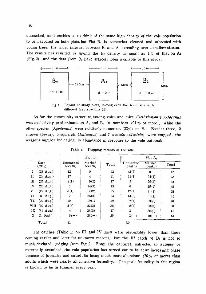
untouched, so it enables us to th ink of the s ame high dens i ty of the vole popula t ion

to be ha rbored on both plots, but Plot Be is s o m e w h a t c leaned and afores ted wi th

young trees, the wide r in te rva l be tween B~ and A, ex t end ing over a shal low s t ream.

The census has resul ted i n g iv ing the ]32 dens i ty as smal l as 1/5 of tha t on A1

(Fig. 2), and the da ta f rom B2 have scarce ly been ava i lab le to this s tudy .

< 60m > " ~ 60m ;, t -60m

B 2 140m ~ 50m~

d = 1 0 m d = 5m d = 10m

)

T 60m

Fig. 1. Layout of study plots, having each the same size with different trap spacings (d).

As for the community structure, among voles and mice, Clethrionornys rufocanus was exclusively predominant on AI and B1 in numbers (91% or more), while the

other species (Apodemus) were relatively numerous (33%) on Bz. Besides those, 2

shrews (Sorex), 5 squi r re ls (Eutarnias) and 7 weasels (Mustela) were t rapped , the

wease l ' s number ind ica t ing i ts abundance in response to the vole ou tbreak .

Table 1. Trapping records of the vole.

Plot B~ Plot A,

Date Unmarked Marked Unmarked Marked (1965) (death) (death) Total (death) (death) Total

I (23 Aug.) II (24 Aug.) III (25 Aug.) IV (26 Aug.) V (27 Aug.) VI (28 Aug.) VII (29 Aug.) VIII (30 Aug.) IX (31 Aug.) X (1 Sept.)

22 17 8(1) 1

8(1) 7

10 8(3) 4 6(--)

0 4 9 (2)

14(3) 17 (2) 26(2) 19(1) 22 (3) 23 (3) 23(--)

22 21 17 15 25 33 29 30 27 29

42 (2) 29(1) 5 6

17(1) 14(5) 7(1) 8(1)

3 3(--)

0 24(1) 29 (2) 29(I) 41 (4) 31 (4) 33 (6) 22 (3) 38(5) 40(--)

42 53 34 35 58

45 40

30 41 43

Total 91 134

T h e ca tches (Table 1) on I I I and IV days were pe rcep t ib ly lower than those

coming ea r l i e r and la te r for unknown reasons , but the I I I ca tch of B1 is not so

much devia ted , judg ing f rom Fig. 2. F r o m the captures , subjec ted to au topsy or

ex t e rna l ly examined , the vole popula t ion has tu rned out to be a t an inc reas ing phase

because of juveni les and subadu l t s be ing much more a b u n d a n t (70 % or more) than

adu l t s which were nea r ly al l in ac t ive fecundi ty . The peak fecundi ty in th is reg ion

is known to be in s u m m e r eve ry year .

95

HOME RANGE

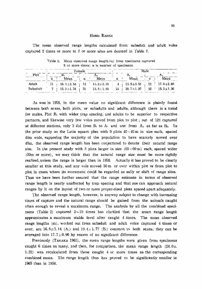
The mean observed range lengths calculated from subadult and adult voles

captured 2 times or more at 2 or more sites are denoted in Table 2.

Table 2. Mean observed range length(m) from specimens captured 2 or more times; n is number of specimens.

Female Male Plot BI A1 B1 A1

n Mean n Mean n Mean n Mean

Adult 11 16.4:k2.54 12 14.2t2.10 4 25. 5!5. 51 12 17.0i2.80 Subadult 7 15. 3• 31 13. 5~:1.55 15 20. 7 t l . 97 32 15. 2 i l . 36

As was in 1958, in the mean value no significant difference is plainly found

between both sexes, both plots, or subadults and adults, although there is a trend

for males, Plot BI with wider trap spacing, and adults to be superior to respective

partners, and likewise very few voles moved from plot to plot ; out of 124 captured

at different stations, only 3 did from B, to A1 and one from A1 as far as B2. In

the prior study on the Latin square plan with 9 plots 40 x 40 m in size each, spaced

40m wide, supposing the majority of the population to have scarcely moved over

40m, the observed range length has been conjectured to denote their natural range

size. In the present study with 3 plots larger in size (60 x60 m) each, spaced wider

(50m or more), we may think that the natural range size must be more tightly

realized, unless the range is larger than in 1958. Actually it has proved to be clearly

smaller at this study, and any vole moved 50 m or over within plot or from plot to

plot in cases where its movement could be regarded as sally or shift of range sites.

Thus we have been further assured that the range estimate in terms of observed

range length is nearly unaffected by trap spacing and that one can approach natural

ranges by it on the layout of two or more proper-sized plots spaced apart adequately.

The observed range length, however, is anyway subject to change with increasing

times of capture and the natural range should be gained from the animals caught

often enough to reveal a maximum range. The analysis by all the combined speci-

mens (Table 2) captured 2--.10 times has clarified that the mean range length

appromixates a maximum stable level after caught 4 times. The mean observed

range lengths (m), worked out from subadult and adult voles captured 4 times or

over, are 16. 8_+1.14 (A1) and 19. 4~=1.77 (B1) common to both sexes; they can be

averaged into 17.7m0.96 by reason of no significant difference.

Previously (TANAKA 1961), the mean range lengths were given from specimens

caught 6 times as many, and then, for comparison, the mean range length (24. O• 1.22) was recalculated from those caught 4 or more times as the corresponding

combined mean. The range length thus has proved to be significantly smaller in

1965 than in 1958.

-96

POPULATION DENSITY

From the trapping record in Table 1, the maximum likelihood estimates and

their standard errors for population parameters were counted by means of the method

and assymptotic variance formulae presented by Dr. SUGIY~.M.~ (TANakA 1954, 1956)

as follows : A

Plot /V p rc

A1 140• 0.30• 0.40•

B~ 110• 0.18+--0. 027 0. 36+-0. 023

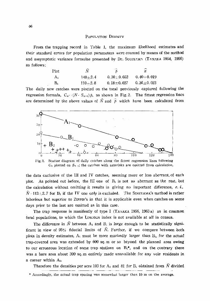
The daily new catches were plotted on the total previously captured following the

regression formula, C . = (N-S,,-,)p, as shown in Fig. 2. The fittest regression lines

are determined by the above values of N and /~ which have been calculated from

o r ,

,

0 20 40 60 80 100 120 140

Fig. 2. Scatter diagram of daily catches along the fittest regression lines following Cr, plotted on S,,-1; the catches with asterisks are omitted from calculation.

the data exclusive of the III and IV catches, seeming more or less aberrant, of each

plot. As pointed out before, the III one of B1 is not so aberrant as the rest, but

the calculation without omitting it results in giving no important difference, e.i . ,

/V=113• for B1 if the IV one only is excluded. The SUGIYAMA'S method is rather

laborious but superior to ZIPPIN'S in that it is applicable even when catches on some

days prior to the last are omitted as in this case.

The trap response is manifestly of type I (TANAKA 1956, 1963 a) as in common

feral populations, to which the LINCOLN index is not available at all in census.

The difference in Pl between A1 and B1 is large enough to be statistically signi-

ficant in view of 95% fiducial limits of _iV. Further, if we compare between both

plots in density estimates, A1 must be more markedly larger than BI, for the actual

trap-covered area was extended by 600 sq. m or so beyond the planned area owing

to our erroneous location of some trap stations on B1 *, and on the contrary there

was a bare area about 300 sq. m entirely made unavailable for any vole residents in

a corner within A1.

Therefore the densities per acre 103 for A1 and 81 for B~ obtained from N divided

* Accordingly, the actual trap spacing was somewhat larger than 10 m on the average.

97

by the designed trap-covered area plus the additional strip area based on the combined

mean range length are incorrect values, and the true density estimates should be

considered as something over 103 for A1 and under 81 for B1.

On the approval of the above consideration, we may remark that the density

estimate on B1 was as small as 70% of that on AI despite the expectation of the

same density on both plots, for which proofs other than a likeness in habitat on

them will be that no significantly different range length was observed and none of

the moved voles did from At to B1.

The reduced estimate will be mainly referable to insufficient exposition of the B1

subpopulation to traps. Then, in case of such a supposed deficiency in trap density,

an effect of multiple collisions of animals with single-catch traps upon iV estimation

has to be considered (TANAKA 1963 b). However it seems unlikely that any signi-

ficant effect was exercised here because any catches on the first 2 days were not

too low.

In conclusion, probably the same density as high as something over 103 existed

on both plots but it was so much underestimated under the design with traps spaced

10 m apart on one plot.

DIscUSSION

With the vole population in the midsummer of 1952, I recognized an appreciable

sexual difference in range size accompanied by a trend of territoriality among adult

females in full breeding activity (TANAKA 1953), whereas no obvious territory was

found in harmony with no sexual difference in range length irrespective of active

fecundity for the present population at an outbreaking density. The failure of

territorial trend might be caused by higher densities*.

The relationship between density and range length resulted from my three studies

can be summarized as follows:

Density level Density (acre) Mean range length(m) ' Year Remarks

61. l:k7.5 (males ) Midsummer Breeding active, Ordinary 15 25. 7 i l . 9 (females) (1952) territory

Ordinary 22 24. 0J=l. 22(both sexes) End of Sept. Breeding no active, (1958) no territory

Outbreaking Something over 103 I7.7i0.96(both sexes) End of Aug. Breeding active, (1965) no territory

From the above, we can remark that at ordinary densities a clear sexual difference

in range length may appear, followed by some territoriality, so long as the breeding

As for only adult females, the density of this year is estimated as about twice of that in 1952, since adults much outnumbered youngs then, their ratio being reversed this year.

98

is very active, while at higher densities it may not even when the fecundity is so

much active. The range length will be depleted by the round amount from 25 to

18 m along with the rise from 20 to 100 in the density level per acre.

Recently the inverse relation of range size with density is acquiring a greater

importance in a census of small rodents, because the density may be more or less

over- or underestimated subject to range size at the time under study ; the undue

estimation is apt to arise either for species having larger ranges or for works with

smaller plots, in particular, with trap lines as discussed by BRANT (1962). In a long

chain of works conducted at tl, t2 ...... , the objective population existing on the initial

plot will be shifted by dint of range size changeable season to season or year to

year, and in consideration of the source of errors we had better count N each time

from daily catches during each work as done here than estimate collectively para-

meters at the successive times by means of equations such as proposed by LESLIE et

al. (1953) and DARROCH (1959). Besides, their methods become largely invalid unless

an isoresponsive population is treated as discussed before (TANAKA 1963a).

The simulation models we have treated (TANAKA 1961, 1966) for the problem of

exposed populations are built up on the assumptions involving disputable i tems;

every animal moving at random over its home range, presumed as a circle of an

average radius (r), is caught with a probability on colliding by chance with a trap

under a grid system of traps spaced d wide, the grid being of boundless extension.

The first difficulty is a random movement all over the range ; a heterogeneous

intensity of use by animals is getting to be of prevalent knowledge. A general

home range of a population might be exhibited by a diagram of the composite ranges,

made up by the superposition of each animal's geometric center of activity, following

a bivariate normal distribution. I have, however, disagreed to the unnatural concept

of home range induced in this way (TANAKA 1963C). MOHR (1965) claiming that

the natural range is elliptic or rectangular rather than circular, has offered a new

procedure to form composite ranges by superposing one over another in an appro-

priate way after fixing long and short axes of each animal. This procedure may

afford a natural shape of home range, whose center is never coincident with the

center of activity in general.

If the circular range is refuted, our model encounters a second difficulty. This

problem has an influence on the usual procedure of density count from 2~ as well.

Then the width, let it be a, of additional strip areas should be revised from

a = n to a ' : l l ' , where l is observed range length or length of long

axis and l' that of short one, supposing the range is rectangular. Nevertheless a is

used in this study presuming that l' is not much smaller than 1. But, if the ratio

l ' / l were greatly variable, the range length could not be a good index of range size.

Lastly, the boundless grid model ignores no simple manner of exposure to traps

99

in animals near or on the border trap lines of plots.

With our model exclusively on a theoretical ground, the unfeasible assumptions

are unavoidable for simplicity; we look forward to a more tenable model. The

hypothesis of CALHOUN (1950) is discordant with our theory in that, we think, the

larger the range, the more traps are there within it and hence the higher does the

probability of capture become.

The simulation experiment of SUGIYAlVtA has proved that x (~r/d) is required to

be 1 or over so as to approximate /Vo, but that of myself, on the same basic assum-

ptions, has shown x=0 .6 to suffice for it (TANAKA 1966). In the work of 1958, /V

was counted as 64• 55• and 50_k4.5 against 2.4, 1.5 and 1.2 for x respec-

tively, since /=24 m, supposing l=2r, is allotted to each case with 5,8 and 10m for

d. The /V-value reveals an inclination to rise with increase of x regardless of no

significant difference among the three cases; that is possibly due to small samples.

Therefore it leaves a suspicion that the largest (64) is nearest to the truth (No).

If the difference should be statistically refutable even in large samples, SUGIYAMA

model could be presumed valid on account of the terms x ~ l sufficing every case.

In the present work, x = l . 8 is given for A1 (d=5m) and 0.89 for B1 (d=10m)

from /=17 .7m, and then, if the model were valid, the density estimates for both

must have made similar to each other, whereas in practice the density on B1 has

been so much underestimated as compared to the supposed true one expressed by

the estimate on A1.

In consideration of the results in 1958 as well as in this time, it seems likely

that the conditions "x is near 2 or more" are strictly required in either ordinary or

outbreaking years in order to get safely to No by means of Aft, because we may

well suppose that the purpose has been achieved only on the terms x = 2 . 4 or 1.8.

Accordingly, so far as our vole, perhaps most of other species of voles (TANAKA

1962), are concerned, the trap-spacing 5m or so is always desirable to know the

whole population in census works. Especially at outbreaks, one could not grasp

their real phase in terms of density if one were to do census on a plan with traps

spaced 10 m or wider. A greater spacing, however, will be allowed to other groups

of mice such as Apodemus and Peromyscus provided with larger ranges.

In this country, a grid composed of 3 traps each set at stations spaced 10 m

apart is usually applied to forecasting census works against vole irruptions, and

thereby, when the three are spaced some distance from one another, it will approach

a 5 m-spacing design.

CONCLUSION

From a field study for the vole population (Clethrionomys rufocanus) in Hokkaido

in the late summer of 1965, it has been proved that the range length may decrease

from 25 to 18 m by the gross along with the rise from 20 to 100 in the density level

100

p e r acre , and h e n c e t h a t an a p p r e c i a b l e d i s c r epancy , due to u n d e r e s t i m a t i o n , m a y be

p r o d u c e d in e s t i m a t e s of t he e x p o s e d as c o m p a r e d to t he who le p o p u l a t i o n a t an

o u t b r e a k i n g d e n s i t y as h i g h as 100 on a p l an w i t h t r a p - s p a c i n g 10 m.

In c o n s i d e r a t i o n of th i s t o g e t h e r w i t h m y p r e c e d i n g resu l t s , t he s t r i c t t e r m s t h a t

we m a y e n o u g h a p p r o x i m a t e t he w h o l e one by e s t i m a t i n g the e x p o s e d s e e m l ike ly

to be t h a t t he ra t io of r a n g e r ad ius to t r ap spac ing , s u p p o s i n g a r a n g e is c i r cu la r ,

shou ld be n e a r 2 o r m o r e a t e i t h e r o r d i n a r y or o u t b r e a k i n g dens i t i e s , to say in t h e

conc re t e , t h a t t he t r ap s p a c i n g as c lose a s 5 m or so in g r id is de s i r ab l e w i t h th i s

vole , p e r h a p s w i t h m o s t o t h e r voles .

ACKNOWLEDGMENT: This is included in the Collective Research "Ecological Study on Population

Dynamics" (Representative : Dr. S. UTIOA) aided by the grant from the Scientific Research

Expenditure, Dept. Education. Besides, I am greatly indebted to Mr. K. TAMVRA, Hokkaido Forest

Protection Society, Dr. K. OTA, Applied Zoology Laboratory, Hokkaido University, and Mr. M. GODA,

Obihiro Governmental Forestry Bureau, for their substantial help to the work.

LITERATURE

BRANT, D.H. (1962) Measures of the movements and population densities of small rodents. Univ.

Calif. Publ. Zool., 62: 105-184.

CAL~OVN, J. B. (1950) North. Amer. Census of Small Mammals, Release. 3.

DARROCrL J. N. (1959) The multiple-recapture census. II. Estimation when there is immigration or

death. Biometrika, 46: 336-351.

L~SLIE, P.H., D. CRtTT~ and H. CmTTY (1953) The estimation of population parameters from data

obtained by means of the capture-recapture method. III. An example of the practical

applications of the method. Biometrika, 40: 137-169.

MOH~, C. (1965) Calculation of area of animal activity by use of median axes and centers in

scatter diagram. Res. Popul. Ecol., 7: 57-72.

TANAKA, R. (1953) Home ranges and territories in a Clethrionornys-population on a peat-bog

grassland in Hokkaido. Bull. Kochi Worn. Coll., 2 : 10-20.

TANAKA, R. (1954) A revised method for estimating reduction of natural populations effected by

poisoning, laP. ]. Sanit. Zool., 4: 186-193.

TANAKA, R. (1956) On differential response to live traps of marked and unmarked small mammals.

Annol. Zool. Jap., 29: 44-61.

TANAKA, R. (1961) A field study of effect of trap spacing upon estimates of ranges and populations

in small mammals by means of a latin square arrangement of quadrats. Bull. Kochi Worn.

Univ., Ser. Nat. Sci., 9: 8-16.

TASAKA, R. (1962) A population ecology of rodent hosts of the scrub-typhus vector of Shikoku

district with special reference to their true range in Japan. ]ap.]. Zool., 13: 395-406.

TANAKA, R. (1963a) On the problem of trap-response types of small mammal populations. Res.

Popul. Ecol., 5 : 139-146.

TANAKA, R. (1963 b) Examination of the routine census equation by considering multiple collisions

with a single-catch trap in small mammals. Jap.]. Ecol., 13: 16-21.

TANAKA, R. (1963 C) Truthfulness of the delimlted-area concept of home range in small mammals.

Bull. Kochi Worn. Univ., Ser. Nat. Sci., 11: 6-11.

101

TANAKA, R. (1964) Recent s t a tu s of r a t infestat ion in the southwest coastal region of Shikoku and

comments on census t rapping of r a t populations. Bull. Kochi Worn. Univ., Ser. Nat. Sci.,

12: 1-8.

T~SAKA, R. (1966) Simulated removal t rapping considered in connection with actual census data in

small mammals . Res. Popul. Ecol., 8:14-19.

Z~PPIN, C. (1956) An evaluat ion of the removal method of es t imat ing animal populations. Biomet-

rics, 12: 163-189.

~-< b%~-~ ~C~,~�9 ~/~'~}]8~CbT~:b. 1965 ~-8~JT~J:~l~_;~tll:kl~j~