a portrait of freshwater fish distribution iparian forests ...€¦ · riparian fish forest on...

Riparian Fish Forest on Haida Gwaii

A Portrait of Freshwater Fish Distribution & Riparian Forestson Haida Gwaii (the Queen Charlotte Islands)

project technical reportby John Broadhead

gowgaia institute2009

published by:Gowgaia InstitutePO Box 638 Queen Charlotte, BC Canada V0T 1S0

A project of Earthlife Canada Foundation

Copyright © 2009 by Gowgaia InstituteAll rights to illustration and text reserved by Gowgaia InstitutePrinted in CanadaFirst printing 2009

Canadian Cataloguing in Publication Data:Main entry under title:RIPARIAN FISH FOREST ON HAIDA GWAII — A Portrait of Freshwater Fish Distribution & Riparian Forests on Haida Gwaii (the Queen Charlotte Islands)

ISBN 0-9687611-1-9URL http://www.spruceroots.org/1. Natural History — Coastal Temperate Rainforest2. Ecology (Riparian Zone Forest, Salmon Habitat, Haida, Logging)3. Land Use Plan, Environmental Condition IndicatorI. Broadhead, John, 1949- II. Leversee, David, 1960-

production

John Broadhead — project director, narrative author, layout, map design Dave Leversee — GIS model & analysis authorLaura Feyrer — GIS agent, research, analysis assistantLynn Lee – fish survey data collection & compilation, model designJoe Lee — GIS programming, database developmentSimon Davies — graphic design

Pen & ink fish drawings by John Broadhead

Contents

Acknowledgements 5

Summary 8

Introduction 10

Data preparation 13

Fish distribution model 20

Mapping the riparian zone 27

Other riparian features 32

Results by ecosections 39

Watershed condition & risk assessment summary 41

References 48

Data sources 50

List of Figures

1. Locations of 456 known waterfalls, boulders, debris slides and other recorded barriers to upstream fish passage.

2. Locations of survey records of 3,705 resident fish and anadromous salmon used in the model.

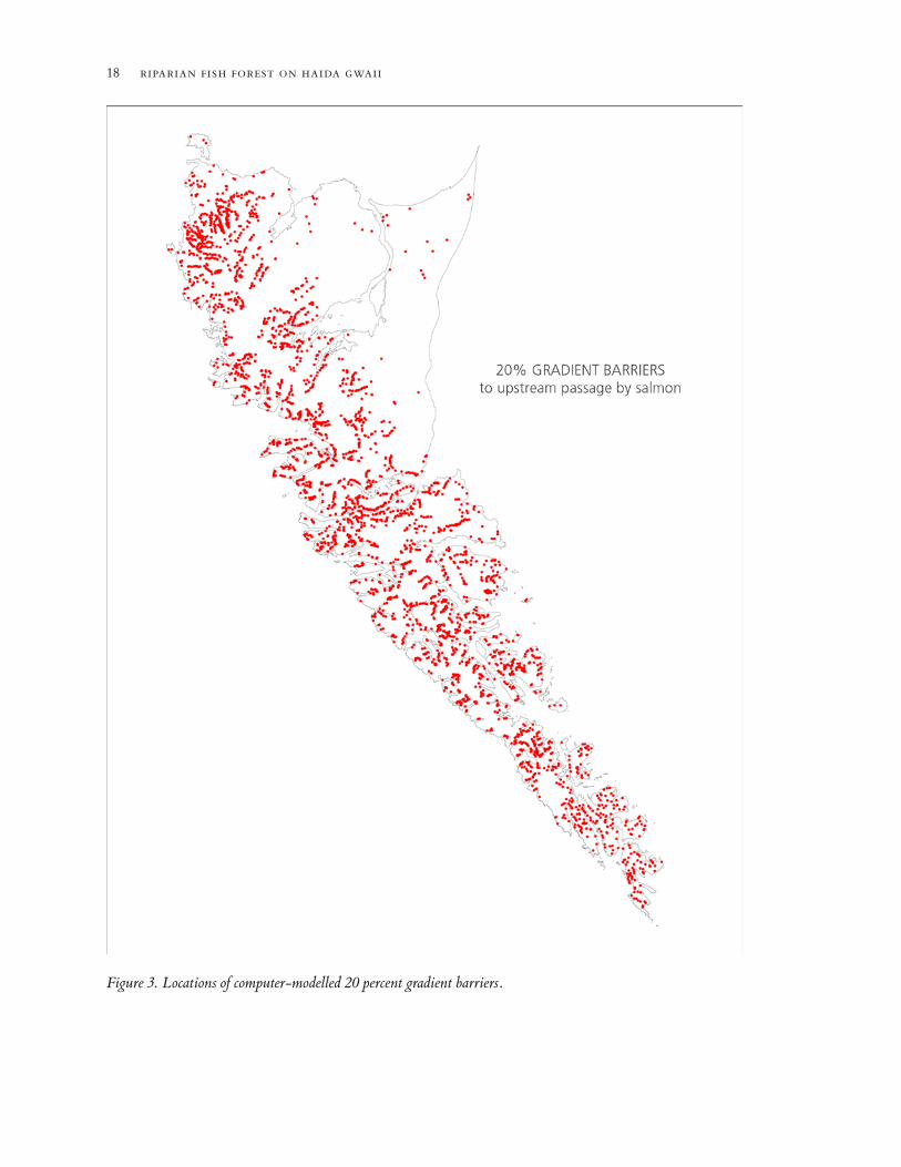
3. Locations of computer-modelled 20 percent gradient barriers.

4. Locations of computer-modelled 30 percent gradient barriers.

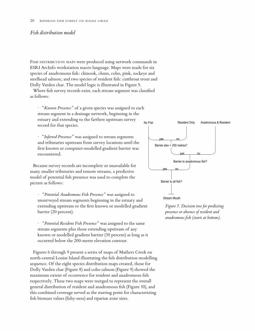
5. Decision tree for predicting presence or absence of resident and anadromous fish.

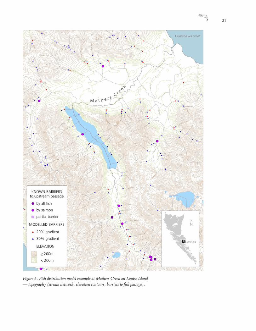
6. Fish distribution model example at Mathers Creek on Louise Island — topography (stream network, elevation contours, barriers to fish passage).

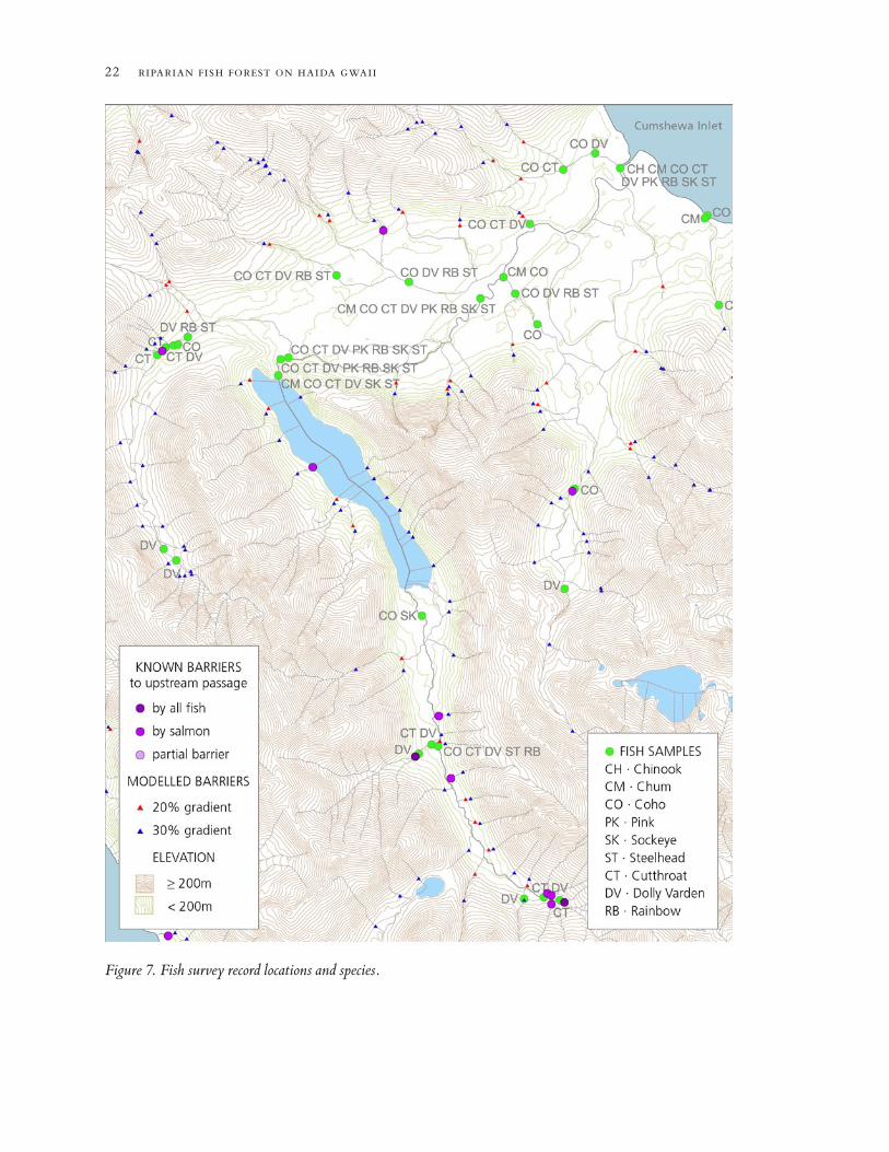
7. Fish survey record locations and species.8. Fish distribution model — result for Dolly Varden char.

4 riparian fish forest on haida gwaii

9. Result for Coho salmon.10. Fish distribution model — summary for all resident and

anadromous fish.11. Fishy-ness classes applied to the summary fish

distribution map.12. Applying stream buffers to fishy-ness classes (see Table 2).13. Extent of Terrestrial Ecosystem Mapping and similar

coverages used to map riparian floodplains.14. All Riparian Fish Forest zones and buffer classes, with

floodplains from Terrestrial Ecosystem Mapping.15. Final map theme for printed poster.16. Final map theme overlaid on an airphoto.17. Riparian Fish Forest poster of all Haida Gwaii (24 x 36

inches).18. Major ecological regions of Haida Gwaii, based on

physiography and climate.19. The big picture — general distribution of climate and

physiographic characteristics affecting fish habitat quality in Haida Gwaii.

20. Watershed risk assessment — indicating the risk that forest conditions important to healthy fish populations have been damaged or destroyed.

List of Tables

1. Summary of anadromous and resident fish species identified from survey records and used in the model.

2. Determining fishy-ness classes and Riparian Fish Forest zone widths based stream magnitude, watershed area, fish occurrence and salmon escapement data.

3. Site series and other Terrestrial Ecosystem Mapping attributes used to theme major riparian floodplain features.

4. Distribution of Riparian Fish Forest classes by ecosection (area in hectares).

5. Logging disturbance and risk assessment of 145 watershed units — based on percentage of forested RFF logged (2006).

6. Risk levels in watersheds associated with the top ten salmon streams.

5

Acknowledgements

For advice on project design and methodology, and for technical review comments at various stages: Alvin Cober, Al Cowan, Marguerite Forest, Rachel Holt, Russ Jones, Peter Katinic, Lynn Lee, Dionys de Leeuw, Michael Milne, Keith Moore, Norm Sloan, Leandre Vigneault.

For access to information or otherwise helping to bring all the pieces together: Pat Bartier, Dan Bate, David Beggs, Alvin Cober, Christina Engel, Pat Fairweather, Victor Fradette, Paul Giroux, Tony Hamilton, Rachel Holt, Jeremy Hyatt, Russ Jones, Peter Katinic, Leah Malkinson, Lynn Miers, Bill Pollard, Frank Reindl, Brian Spilsted, John Sunde, Dave Trim, Leandre Vigneault.

For lending their personal expertise and experience of fish and streams to the critical task of error-checking the map: Alvin Cober, George Farrell, Jeremy Hyatt, Peter Katinic, Lynn Lee, Keith Moore, Tom Reimchen, Frank Reindl, Leandre Vigneault, Mark Walsh.

For explaining the relationship between Tsiin (salmon) and everything else, and Yah’gudang (respect) as the ‘prime directive’: Arnie Bellis, Tim Boyko, Carrie Carty, Vince Collison, Nika Collison, Margaret Edgars, Guujaaw, Russ Jones, Tamara Rullin, Ed Russ, Elsie Stewart-Burton, Alan Wilson and so many more Xaayda laas.

Thank you everyone who helped out along the way over the past four years. In spite of your own best efforts, any errors or omissions in this report are mine.

Haaw’a JB

With financial support from:

The Bullitt FoundationCoast Sustainability TrustGordon & Betty Moore FoundationGwaii Forest SocietySouth Moresby Forest Replacement AccountThe W. Alton Jones FoundationThe William & Flora Hewlett Foundation Mapping Fund in Tides Canada FoundationWorld Wildlife Fund (Canada) — thank you Glen Davis

In memory of Charlie Bellis — Skil Ku’das of the Yaku ‘laanaas Raven clan —

who loved to fish, to share the ocean’s bounty and his knowledge of its ways, who said:

Salmon are creatures of the forest.They’re born in the forest

and it’s in the forest that they die.


Summary

Most of the people involved in a recent Land Use Plan (LUP) process on Haida Gwaii agreed that salmon and the riparian forests around freshwater streams are a key indicator of environmental condition, and so also the health and well-being of the people who depend on fish and forests for economic and cultural sustenance.

The members of the Community Planning Forum voiced concern about the accumulated and ongoing impacts of the past fifty years of logging. People wanted to account for the disturbance, to indentify the problem areas, the salmon populations at risk, and to create appropriate forest management objectives to protect and restore them.

The problem was there was no landscape-scale map of where fish actually do and don’t go in the islands’ several thousand lakes and streams, nor of the riparian habitats that surround them, nor of the places where logging has disturbed them. Most of the information needed to make such a map existed, but it was widely scattered: created by different authors in different agencies for different reasons, at different scales and in different print and digital formats.

The solution was this project by the Gowgaia Institute, in con-sultation with the LUP Process Technical Team, to assemble as much of the relevant information as possible within a single geographic framework for analysis — a portrait of the distribution of salmon and other freshwater fish and the riparian forest around them.

We used a computer geographic information system (GIS) to combine a 1:20,000 scale network model of streams and lakes with various other maps and databases produced at scales ranging from 1:5,000 to 1:250,000. Some 1,782 fish survey records identifying 14 species of resident and anadromous fish collected in traps at various locations were linked to points in the network, as were 456 known waterfalls and other barriers to upstream fish passage, plus 15,327 computer-modelled gradient barriers. Salmon spawning escapement data collected over the past fifty years for five species of salmon in 335 streams were merged with the network model through stream ID codes.

Once the data tables were assembled and cleaned, we used GIS queries (network commands in ESRI ArcInfo workstation macro language) to map the known and inferred presence and absence of eight species of anadromous and resident freshwater fish within the network of streams and lakes. The model was refined through an iterative process of identifying known errors, correcting database features and adjusting GIS query parameters to achieve the best fit. A series of draft maps were reviewed by ten local experts with

9

wide-ranging field experience. Remotely sensed imagery and local geographic references were also reviewed and used to inform adjustments to the map as appropriate.

The next step was to combine these fish distribution maps with data regarding stream magnitude, watershed size and salmon abundance in order to estimate the general productivity of fish and forest biomass in the riparian forest zone surrounding any given waterway. We created a rankings table with seven classes of fishy-ness ranging from no fish at all in the highest and steepest streams, through to most salmon in the biggest, most productive systems.

Depending on its fishy-ness class, each line segment defining a waterway received a radial map buffer to approximate the extent of its Riparian Fish Forest zone, ranging from 20m for no fish to 80m for most salmon — thus representing the range of biological productivity in riparian forest stands from lower biomass levels in small riparian ecosystems with few fish, to higher biomass levels in larger, more complex riparian ecosystems with many fish.

Finally, major riparian floodplain features identified in 1:20,000 scale terrestrial ecosystem maps (TEM) were merged with the fishy-ness index maps into a single coverage for the entire, one million-hectare (3,860 square mile) archipelago. The map of Riparian Fish Forest on Haida Gwaii is available in various print and digital formats and sizes at www.spruceroots.org, including a GoogleEarth-ready file.

In 2005, the Riparian Fish Forest (RFF) coverage was used by the team of technical analysts for the Haida Gwaii Land Use Plan as one of several indicators of environmental condition — by comparing the riparian map with the islands’ logging history and so measuring the spatial extent of disturbance. The Environmental Conditions Report includes an assessment of environmental risk and restoration priorities in 145 watershed units on the archipelago. A slightly modified Summary of Watershed Condition is appended to this report.

The Haida Gwaii Strategic Land Use Agreement (SLUA) was signed by the Province of British Columbia and Council of the Haida Nation on 12 December 2007. In 2007–08, the RFF fish distribution data have helped various agency analysts identify High Value Fish Habitat associated with new Ecosystem-Based Management (EBM) Objectives for protecting Aquatic Habitats. Likewise, the RFF Risk Assessment has helped to identify Sensitive Watersheds where logging should be curtailed in favour of a period of hydrological recovery.


Introduction

Haida Gwaii, also called the Queen Charlotte Islands, is an isolated archipelago in the northeast Pacific Ocean, centred on longitude 132° west and latitude 53° north, about 100 kilometres from the British Columbia mainland coast. It’s a collection of 350 islands, large and small, totalling about a million hectares in size and arrayed in a long, triangular shape that from space resembles a giant scimitar laying partly submerged at the western edge of Canada’s continental shelf.

In ecological terms, the islands are part of the globally rare Coastal Temperate Rainforest biome, regionally classified as the Coastal Western Hemlock biogeoclimatic zone, and locally discernable into “wet and very wet hyper-maritime” variations. There are many freshwater wetlands of bog, fen, marsh and swamp, with flat, raised and blanket bogs being especially conspicuous. Subalpine and alpine zones are not extensive, but contain biologically distinctive vascular plant species.

The influence of the ocean is pervasive. With over four thousand kilometres of inlet and island shorelines, over 25 percent of the archipelago’s “interior” is within one kilometre of saltwater, and no place is further than 20 kilometres from the sea. Pacific weather systems deliver up to five metres of precipitation per year on the windward west coast and one metre on the more sheltered east coast, mostly rain, which collects and courses through thousands of streams, lakes and bogs on its way back to the sea.

Complementing the sheer physical connectivity between land and sea provided by all that water, there are fourteen kinds of fish swimming in the archipelago’s streams and lakes, including resident and anadromous forms of sockeye, coho, chum, pink and chinook salmon, steelhead, rainbow and cutthroat trout, dolly varden char, stickleback, sculpin and lamprey. The anadromous salmon in particular are a key source of nutrients transferred from marine food webs to the forest on land, and are now recognized as a major factor in the relatively high productivity of riparian forest ecosystems adjacent to salmon spawning streams (Reimchen 2004).

Haida Gwaii is the most isolated land mass in Canada, slightly closer to Alaska than to British Columbia. This satellite image was made with data collected on June 13, 2002 by the NASA Earth Observatory SeaWIFS Project, and is enhanced with information about marine plant life to reveal several large ocean eddies formed by freshwater run-off from mainland rivers.

11

One aspect of this productivity of course is trees, big trees, and the forests of Haida Gwaii are noted for growing particularly large and valuable specimens of Sitka spruce, western red cedar, western hemlock and yellow cypress. Over the past hundred years of industrial logging, extensive tracts of old growth forest have been removed from valley bottoms and hillsides (Broadhead and Leversee 2004), resulting in significant damage to riparian areas, and coinciding with observed declines in salmon populations over the last half century (Riddel 2004).

In April 2001, the province of British Columbia and the Haida Nation signed the Protocol Agreement on Interim Measures & Land Use Planning for Haida Gwaii, the purpose of which was to jointly produce a strategic Land Use Plan — also known as a Land & Resource Management Plan (LRMP). The plan was to include a system of protected natural areas plus objectives for “ecosystem-based management” of logging and other industrial uses, including the restoration and renewal of forest ecosystems.

In legal parlance it would be a “higher level” plan, meaning that its terms and conditions, once established in law, could supersede the status quo legislation and management regulations. Thus the economic and environmental stakes were high, depending on the degree to which the plan might attempt to reduce environmental risk by establishing reserves to protect or restore damaged ecosystems, or otherwise reduce the rate of logging.

The agreement also stipulated that the Haida would provide a foundation document to guide the process called the Haida Land Use Vision (HLUV) — which would describe Haida concerns and objectives for restoring environmental well-being and maintaining Haida culture through a land use plan (CHN 2004).

A Community Planning Forum (CPF) was convened, consisting of several dozen representatives for the Haida, the province, industry, and other social sectors with an interest in the plan. The forum met periodically between September 2003 and February 2005 with a mandate to recommend the strategic elements and objectives of an “ecosystem-based” land use plan for the archipelago.

A Process Technical Team (PTT), consisting of technical experts from provincial and Haida government agencies, industry and NGOs, worked from January 2003 to March 2005 on various economic and ecological reports and maps in support of the planning forum at various stages in its deliberations.

With over four thousand kilometres of inlet and island shorelines, over 25 percent of the archipelago’s “interior” is within one kilometre of saltwater, and, even on the largest island (Graham), no place is further than 20 kilometres from the sea.


From the outset, the well-being of salmon was identified by all as a critical issue. The PTT identified freshwater fish habitat and riparian forests as a key indicator of environmental condition and a high priority information gap to address. The HLUV identified watersheds with culturally significant salmon runs in urgent need of protection and restoration. The CPF requested explicit information about where freshwater streams and lakes are actually occupied by fish (or not), and to what extent they have been disturbed by logging.

As a first step, the Nature Conservancy of Canada had proposed to the PTT to classify freshwater ecosystems with a computer model based on soils, hydrology and other physical features, but cautioned that a lack of adequate survey data for freshwater species might limit its usefulness. A preliminary draft map was reviewed by the PTT and found to be overly generalized and inconsistent with local knowledge of fish and stream characteristics, and so of limited usefulness.

What was needed was a mapping tool broad enough in scope to show relevant landscape level patterns at a glance, yet accurate enough in detail to read as true to local experts. The map would need to combine fish survey data with a network model of streams and lakes, elevation contours, local forest ecosystem features and logging history, all of which were available but had been produced by different authors at different scales for different end uses.

The Gowgaia Institute, a local NGO participant in the Process Technical Team with locally-established GIS capacity, was tasked to work in consultation with the PTT and other local experts to create a 1:20,000 scale model of sufficient accuracy for landscape-level planning, and to illustrate and quantify three things:

· the distribution of fish in freshwater streams and lakes;

· the spatial pattern of the riparian forest zone; and

· environmental disturbance and risk caused by logging.

This report describes how the field survey data and other map elements were collected, combined and themed to produce the final single map coverage called Riparian Fish Forest on Haida Gwaii, and so fulfilling the first two objectives.

The third objective above is reported in detail in “Environmental Conditions Report for the Haida Gwaii Queen Charlotte Islands Land Use Plan, Chapter 2.3 — Watershed Condition” (Holt 2005) prepared by Rachel Holt with the Process Technical Team. A brief summary is presented later in this report.

13

Data preparation

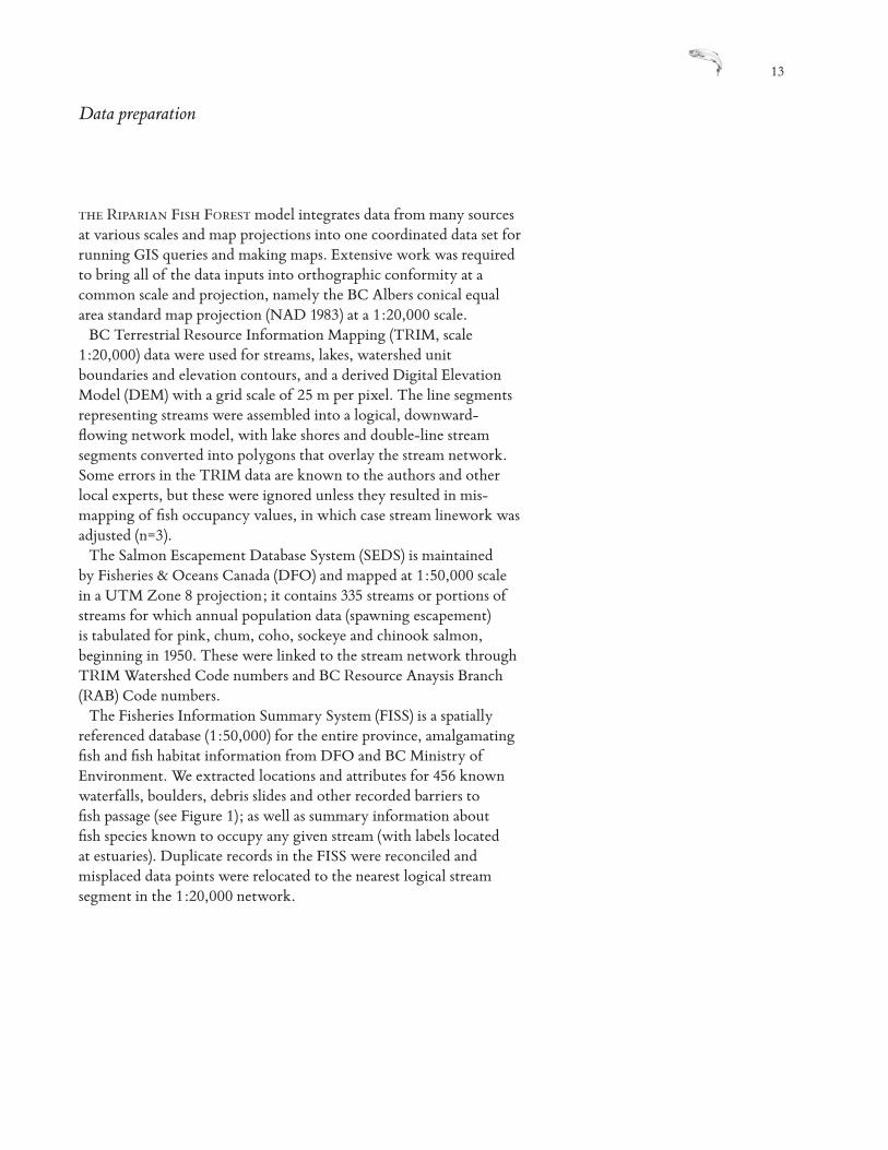
the Riparian Fish Forest model integrates data from many sources at various scales and map projections into one coordinated data set for running GIS queries and making maps. Extensive work was required to bring all of the data inputs into orthographic conformity at a common scale and projection, namely the BC Albers conical equal area standard map projection (NAD 1983) at a 1:20,000 scale.

BC Terrestrial Resource Information Mapping (TRIM, scale 1:20,000) data were used for streams, lakes, watershed unit boundaries and elevation contours, and a derived Digital Elevation Model (DEM) with a grid scale of 25 m per pixel. The line segments representing streams were assembled into a logical, downward-flowing network model, with lake shores and double-line stream segments converted into polygons that overlay the stream network. Some errors in the TRIM data are known to the authors and other local experts, but these were ignored unless they resulted in mis-mapping of fish occupancy values, in which case stream linework was adjusted (n=3).

The Salmon Escapement Database System (SEDS) is maintained by Fisheries & Oceans Canada (DFO) and mapped at 1:50,000 scale in a UTM Zone 8 projection; it contains 335 streams or portions of streams for which annual population data (spawning escapement) is tabulated for pink, chum, coho, sockeye and chinook salmon, beginning in 1950. These were linked to the stream network through TRIM Watershed Code numbers and BC Resource Anaysis Branch (RAB) Code numbers.

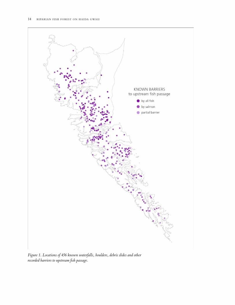
The Fisheries Information Summary System (FISS) is a spatially referenced database (1:50,000) for the entire province, amalgamating fish and fish habitat information from DFO and BC Ministry of Environment. We extracted locations and attributes for 456 known waterfalls, boulders, debris slides and other recorded barriers to fish passage (see Figure 1); as well as summary information about fish species known to occupy any given stream (with labels located at estuaries). Duplicate records in the FISS were reconciled and misplaced data points were relocated to the nearest logical stream segment in the 1:20,000 network.


Figure 1. Locations of 456 known waterfalls, boulders, debris slides and other recorded barriers to upstream fish passage.

15

Other sources of information about fish species presence and barriers to fish passage included the BC Watershed Atlas (1:50,000) and 1,782 fish survey records (mostly 1:5,000) containing 3,705 individual salmonids, char, sculpin, stickleback and lamprey obtained from hardcopy reports, digital maps and catalogues commissioned by DFO, Parks Canada, the Haida Fisheries Program, non-governmental agencies, fisheries contractors and timber licensees (see Table 1 and Figure 2). These reports also included some detailed local knowledge about barriers to fish movement not contained in the fisheries data-bases mentioned above. Point location records were digitized and georeferenced if necessary, and then all merged into a single coverage overlaid on the 1:20,000 scale TRIM stream network.

Many of the 1:5,000 scale fish sample surveys identify small stream features that either vary to some extent with, or are not present in, the 1:20,000 TRIM map. In the case of non-conforming stream channel locations, we tied survey points to the nearest appropriate TRIM stream segment. In the case of small streams not present in the TRIM data, we tied survey points to the closest TRIM stream segment to which the 1:5,000 scale stream would likely be a tribu-tary. This was a time-consuming task, but essential to creating a viable model topology.

Table 1. Summary of anadromous and resident fish species identified from survey records and used in the model.

Anadromous

14 Salmonidae Chinook Salmon Oncorhynchus tshawytscha421 Salmonidae Chum Salmon Oncorhynchus keta957 Salmonidae Coho Salmon Oncorhynchus kisutch345 Salmonidae Pink Salmon Oncorhynchus gorbuscha102 Salmonidae Sockeye Salmon Oncorhynchus nerka116 Salmonidae Steelhead Oncorhynchus mykiss466 Salmonidae Cutthroat Trout Oncorhynchus clarki 4 Salmonidae Kokanee Oncorhynchus nerka

171 Salmonidae Rainbow Trout Oncorhynchus mykiss 32 Salmonidae Trout (General Oncorhynchus sp.864 Salmonidae Dolly Varden Salvelinus malma 2 Petromyzontidae Pacific Lamprey Lampetra tridentata 44 Cottidae Coastrange Sculpin Cottus aleuticus 27 Cottidae Prickly Sculpin Cottus asper 30 Cottidae Sculpins (General) Cottus sp.110 Gasterosteidae Threespine Stickleback Gasterosteus aculeatus

Count Family Common name Species

Resident

A total of 3,705 fish were collected and counted in 1,782 survey records.


Figure 2. Locations of survey records of 3,705 resident fish and anadromous salmon used in the model.

17

In locations where no survey data for fish or barriers were available, we developed a method for predicting their presence or absence based on stream gradient and elevation. We used a GIS routine to intersect the TRIM stream network with elevation contours and calculate the gradients of over 40,000 stream segments. Where stream initiation points and junctions occurred between elevation contours, we used a 25-metre Digital Elevation Model (MEMPR 2004) to calculate gradient values. A total of 15,327 gradient barriers were established (see Figures 3 and 4), based on the following assumptions:

· Modelled gradient barriers – For anadromous salmon, these were located at the lowest point of a stream segment having a calculated slope of over 20 percent; for resident species, when the slope was over 30 percent. The gradient value selected for anadromous species is consistent with the guidelines for determining fish presence as outlined in the Riparian Management Area Guidebook (Ministry of Forests 1995). The value for resident species was adjusted in order to conform with local survey information, where fish have been caught in step-pool streams with gradients of up to 27 percent (Lee 2004).

· Distribution of resident fish – Cutthroat and rainbow trout and Dolly Varden char are commonly caught upstream of barriers to anadromous fish, and it is believed that they could readily disperse below this type of barrier. The model assumed that resident fish exist downstream of such barriers if the upstream reach has known or inferred resident fish present. If the stream above such a barrier is of a consistently low gradient, the model assumed that resident fish are able to travel upstream until they encounter a 30 percent gradient barrier.

· A 200-metre barrier/elevation limit – Given the total absence of fish recorded in surveys upstream of barriers higher than 200 metres, the model assumed that resident fish distribution could not be inferred beyond barriers located at or above this elevation, regardless of stream gradient (ibid.).


Figure 3. Locations of computer-modelled 20 percent gradient barriers.

19

Figure 4. Locations of computer-modelled 30 percent gradient barriers.


Fish distribution model

Fish distribution maps were produced using network commands in ESRI ArcInfo workstation macro language. Maps were made for six species of anadromous fish: chinook, chum, coho, pink, sockeye and steelhead salmon; and two species of resident fish: cutthroat trout and Dolly Varden char. The model logic is illustrated in Figure 5.

Where fish survey records exist, each stream segment was classified as follows:

· “Known Presence” of a given species was assigned to each stream segment in a drainage network, beginning in the estuary and extending to the farthest upstream survey record for that species.

· “Inferred Presence” was assigned to stream segments and tributaries upstream from survey locations until the first known or computer-modelled gradient barrier was encountered.

Because survey records are incomplete or unavailable for many smaller tributaries and remote streams, a predictive model of potential fish presence was used to complete the picture as follows:

· “Potential Anadromous Fish Presence” was assigned to unsurveyed stream segments beginning in the estuary and extending upstream to the first known or modelled gradient barrier (20 percent).

· “Potential Resident Fish Presence” was assigned to the same stream segments plus those extending upstream of any known or modelled gradient barrier (30 percent) as long as it occurred below the 200-metre elevation contour.

Figures 6 through 9 present a series of maps of Mathers Creek on north-central Louise Island illustrating the fish distribution modelling sequence. Of the eight species distribution maps created, those for Dolly Varden char (Figure 8) and coho salmon (Figure 9) showed the maximum extent of occurrence for resident and anadromous fish respectively. These two maps were merged to represent the overall general distribution of resident and anadromous fish (Figure 10), and this combined coverage served as the starting point for characterizing fish biomass values (fishy-ness) and riparian zone sizes.

no

Anadromous & Resident

Barrier to all fish?

Stream Mouth

yes

noyes

yes no

No Fish Resident Only

Barrier to anadromous fish?

Barrier elev > 200 metres?

Figure 5. Decision tree for predicting presence or absence of resident and anadromous fish (starts at bottom).

21

Figure 6. Fish distribution model example at Mathers Creek on Louise Island — topography (stream network, elevation contours, barriers to fish passage).


Figure 7. Fish survey record locations and species.

23

Figure 8. Fish distribution model — result for Dolly Varden char.


Figure 9. Result for coho salmon.

25

Figure 10. Fish distribution model — summary for all resident and anadromous fish.


The next step was an iterative process of identifying errors, correcting database features and adjusting GIS query parameters to achieve the best fit between known information and the model. Ten fish biology experts with wide-ranging local field experience reviewed a series of preliminary maps similar to Figure 10 for accuracy in displaying fish presence or absence (see Acknowledgements for list of experts). Digital air photos (0.7 m per pixel) were used where possible to corroborate recommended adjustments to barriers and fish occurrences, as were other locally relevant references (Dalzell 1973; Northcote et al. 1989; Reimchen 1992). Most corrections were for unrecorded barriers that were not identified by the stream gradient model due to the scale of the TRIM elevation data, but were known to the local experts (n=22). One correction was made where the FISS database indicated a barrier to anadromous fish that does not exist.

Of the 1,782 fish sample points used, 28 did not agree with the model, the majority of which represented resident fish that had been recorded above gradient barriers that were slightly steeper than the model’s 30 percent limit. The sum of stream segment lengths affected by these 28 discrepancies was 8 kilometres — less than one tenth of one percent of the total length of all stream segments in the model.

27

Mapping the riparian zone

“Every year the salmon swim into the forest to spawn, carrying in their bodies thousands of tonnes of nutrients gathered in ocean food webs, back to the land … Black bear snatch tens of thousands of salmon out of the streams and haul them onto the forest floor … Eventually the nutrients within their bodies pass into the soil and from there to the roots of trees and plants. The salmon feed the forest and in return receive clean water and gravel in which to hatch and grow, sheltered from extremes of temperature and water flow in times of high and low rainfall.” Haida Land Use Vision (CHN 2004)

Having created a landscape-scale map of where fish actually do and don’t swim in the lakes and streams of Haida Gwaii, the next step was to map the riparian zone around them. To be relevant to the concerns raised by the Haida and other members of the Community Planning Forum, we needed to delineate the streamside places where water, plants, soil, insects and mammals are directly linked to the life cycles of Pacific salmon and the other freshwater fish.

The word “riparian” — from the Latin ripa, meaning bank — has long been used to refer to the ecotone along the banks of streams and rivers. Over time, scientists have articulated a wide range of ecological features in riparian zones, and the definition has broadened to include the shores of lakes and salt-water bodies. Some call it the hydroriparian zone of influence, referring to all of the ways that terrain, animals, vegetation, soil and microclimate interact with and are influenced by perennial, intermittent and occult occurances of water, and vice versa (Price and McLennan 2001).

Generally speaking, the more water there is in a stream, the more extensive is the hydroriparian zone of influence. And, riparian forests that grow around streams and lakes with fish in them are larger and richer, with more biological diversity, bigger trees and more accumulated biomass — the richest ones having the most salmon in them (Naiman et al. 2000; Reimchen 2004). Depending on which aspect of a riparian zone is considered, from leaf litter dropping into small hillside tributaries to bears hauling salmon out of a stream and into the relative security of the adjacent forest, the physical extent of detectable influences ranges anywhere from a few to several hundred metres.

Because the primary use of the Riparian Fish Forest (RFF) model would be as an indicator of environmental condition, and because the results were sure to provoke close scrutiny by all parties concerned with the implications for land use and forest management, it was


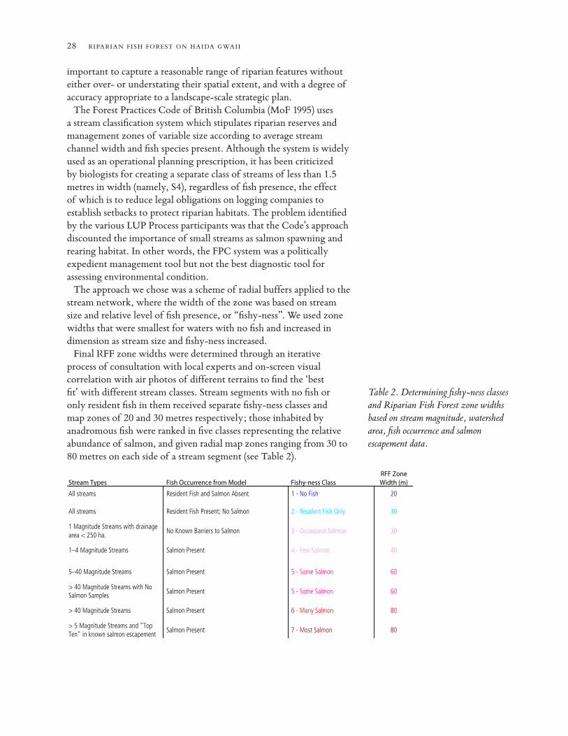
important to capture a reasonable range of riparian features without either over- or understating their spatial extent, and with a degree of accuracy appropriate to a landscape-scale strategic plan.

The Forest Practices Code of British Columbia (MoF 1995) uses a stream classification system which stipulates riparian reserves and management zones of variable size according to average stream channel width and fish species present. Although the system is widely used as an operational planning prescription, it has been criticized by biologists for creating a separate class of streams of less than 1.5 metres in width (namely, S4), regardless of fish presence, the effect of which is to reduce legal obligations on logging companies to establish setbacks to protect riparian habitats. The problem identified by the various LUP Process participants was that the Code’s approach discounted the importance of small streams as salmon spawning and rearing habitat. In other words, the FPC system was a politically expedient management tool but not the best diagnostic tool for assessing environmental condition.

The approach we chose was a scheme of radial buffers applied to the stream network, where the width of the zone was based on stream size and relative level of fish presence, or “fishy-ness”. We used zone widths that were smallest for waters with no fish and increased in dimension as stream size and fishy-ness increased.

Final RFF zone widths were determined through an iterative process of consultation with local experts and on-screen visual correlation with air photos of different terrains to find the ‘best fit’ with different stream classes. Stream segments with no fish or only resident fish in them received separate fishy-ness classes and map zones of 20 and 30 metres respectively; those inhabited by anadromous fish were ranked in five classes representing the relative abundance of salmon, and given radial map zones ranging from 30 to 80 metres on each side of a stream segment (see Table 2).

Table 2. Determining fishy-ness classes and Riparian Fish Forest zone widths based on stream magnitude, watershed area, fish occurrence and salmon escapement data.

Stream Types Fish Occurrence from Model Fishy-ness ClassRFF Zone Width (m)

All streams Resident Fish and Salmon Absent 1 - No Fish 20

All streams Resident Fish Present; No Salmon 2 - Resident Fish Only 30

1 Magnitude Streams with drainage area < 250 ha.

No Known Barriers to Salmon 3 - Occasional Salmon 30

1–4 Magnitude Streams Salmon Present 4 - Few Salmon 40

5–40 Magnitude Streams Salmon Present 5 - Some Salmon 60

> 40 Magnitude Streams with No Salmon Samples Salmon Present 5 - Some Salmon 60

> 40 Magnitude Streams Salmon Present 6 - Many Salmon 80

> 5 Magnitude Streams and "Top Ten" in known salmon escapement

Salmon Present 7 - Most Salmon 80

29

Salmon streams were stratified for relative fishy-ness using a combination of stream size, drainage area, and spawning escapement data. Stream magnitude (i.e. the number of tributaries occurring upstream of any given stream segment) was used to indicate size, and watershed drainage area was used to isolate very small streams with seasonally intermittent flows. The most appropriate magnitude and watershed area divisions were determined through an iterative sensitivity analysis in consultation with local experts.

The initial step was to divide salmon systems into three classes — “few salmon” (magnitude 1 to 4), “some salmon” (magnitude 5 to 40), and “many salmon” (magnitude over 40). Three subdivisions were created to reflect local circumstances including: small, low-flow streams; apparently suitable streams with no known records of salmon occupancy; and streams known to support relatively large salmon populations.

In the first instance, small headwater and low-flow streams are less productive fish habitat, so we downgraded any magnitude-1 stream that drains a watershed with an area of less than 250 hectares from “few salmon” to “occasional salmon.” These are very small streams with no tributaries and seasonally intermittent flows, but otherwise no apparent barriers to salmon. They occur on low gradient terrain throughout the islands, but the majority are found in the flat, muskeg-covered terrain of north central and northeast Graham Island, where they are known to be inhabited occasionally by relatively small numbers of coho salmon.

Secondly, five larger systems (i.e. > magnitude 40) draining the western side of northwest Graham Island were classified by the model as “many salmon” because of their size, yet there are no survey records to indicate the presence of salmon runs in them. Assuming that any significant salmon populations would have been previously identified as such, we downgraded these five systems from “many salmon” to “some salmon.”

Finally, DFO salmon escapement data (SEDS) were sorted to identify the top ten producers of pink, chum, coho, sockeye and chinook salmon. Twenty-five streams were identified as having one or more species in the top ten and so were upgraded to “class 7-most salmon” — 23 of these were upgraded from “class 6-many salmon,” two from “class 5-some salmon.”

The resulting theme of fishy-ness classes for Mathers Creek on Louise Island are illustrated in Figure 11. The application of Riparian Fish Forest buffer widths from Table 2 is illustrated in Figure 12.


Figure 11. Fishy-ness classes applied to the summary fish distribution map.

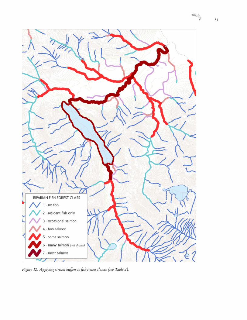
31

Figure 12. Applying stream buffers to fishy-ness classes (see Table 2).


Other riparian features

While stream banks and lake shores with a direct physical connection to fish habitat are well represented in the TRIM stream network, some other important features of the hydroriparian zone of influence — headwaters and floodplains — are not.

Headwater (or first order) streams typically comprise more than one half of a watershed’s total catchment area and play a major ecological role in providing sediment, water, nutrients and organic matter for downstream reaches (Gomi et al. 2002). Yet despite their large aggregate area and major influence on the health and vitality of a watershed, they are often overlooked as riparian features because they are small, complex and not always occupied by fish (ibid.). Where they have been mapped on Haida Gwaii, most were made in the context of operational plans for logging at a 1:5,000 scale, and only in places where detailed mapping has been required by law over the past 14 years or so. We concluded that it was not feasible to create or incorporate a comprehensive coverage of headwater features in the RFF model, which as a consequence understates their spatial and ecological significance.

Riparian floodplains are another important aspect of fish habitat that called for special mapping treatment, in this case with more success than headwaters. At the time the RFF model was produced, about 55 percent of Haida Gwaii was subject to some form of ecosystem mapping suitable for representing major floodplain features (see Figure 13). While this provided a less than complete coverage, our approach was to create a mosaic of the best available data in any given region to build as clear and comprehensive a picture of riparian floodplains as possible.

Terrestrial Ecosystem Mapping (TEM) at a 1:20,000 scale was available for TFL 39–Block 6 and parts of the Queen Charlotte Timber Supply Area (Ministry of Environment 1995-2004). These ecosystem unit polygons were drawn using air photo interpretation (Clement 2004) and verified through field surveys to confirm site series classifications (Green and Klinka 1994) and describe dominant plants, soils, humus and surficial geology (Clement 1995).

A similar terrain unit mapping product was available in TFL 47 and 25 — a precursor to Vegetation Resource Inventory mapping produced by methods similar to TEM (Lewis 1981, 2003). We used a crosswalk table to translate these terrain/ecosystem units into site series classifications with attribute tables similar to those available in the TEM, at which point we were able to query both mapping products for riparian floodplain features.

Source TEM

Lewis

Figure 13. Extent of Terrestrial Ecosystem Mapping and similar coverages used to map riparian floodplains.

33

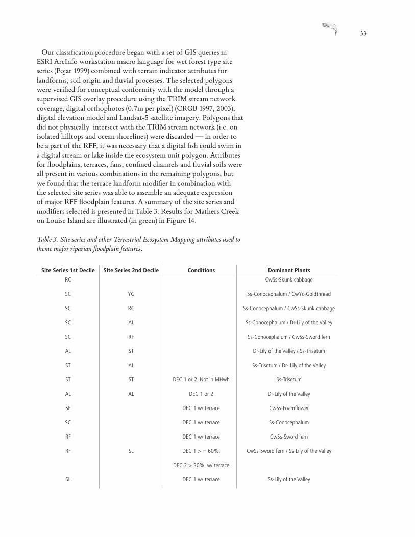
Our classification procedure began with a set of GIS queries in ESRI ArcInfo workstation macro language for wet forest type site series (Pojar 1999) combined with terrain indicator attributes for landforms, soil origin and fluvial processes. The selected polygons were verified for conceptual conformity with the model through a supervised GIS overlay procedure using the TRIM stream network coverage, digital orthophotos (0.7m per pixel) (CRGB 1997, 2003), digital elevation model and Landsat-5 satellite imagery. Polygons that did not physically intersect with the TRIM stream network (i.e. on isolated hilltops and ocean shorelines) were discarded — in order to be a part of the RFF, it was necessary that a digital fish could swim in a digital stream or lake inside the ecosystem unit polygon. Attributes for floodplains, terraces, fans, confined channels and fluvial soils were all present in various combinations in the remaining polygons, but we found that the terrace landform modifier in combination with the selected site series was able to assemble an adequate expression of major RFF floodplain features. A summary of the site series and modifiers selected is presented in Table 3. Results for Mathers Creek on Louise Island are illustrated (in green) in Figure 14.

Table 3. Site series and other Terrestrial Ecosystem Mapping attributes used to theme major riparian floodplain features.

Site Series 1st Decile Site Series 2nd Decile Conditions Dominant Plants

RC CwSs-Skunk cabbage

SC YG Ss-Conocephalum / CwYc-Goldthread

SC RC Ss-Conocephalum / CwSs-Skunk cabbage

SC AL Ss-Conocephalum / Dr-Lily of the Valley

SC RF Ss-Conocephalum / CwSs-Sword fern

AL ST Dr-Lily of the Valley / Ss-Trisetum

ST AL Ss-Trisetum / Dr- Lily of the Valley

ST ST DEC 1 or 2. Not in MHwh Ss-Trisetum

AL AL DEC 1 or 2 Dr-Lily of the Valley

SF DEC 1 w/ terrace CwSs-Foamflower

SC DEC 1 w/ terrace Ss-Conocephalum

RF DEC 1 w/ terrace CwSs-Sword fern

RF SL DEC 1 > = 60%, CwSs-Sword fern / Ss-Lily of the Valley

DEC 2 > 30%, w/ terrace

SL DEC 1 w/ terrace Ss-Lily of the Valley


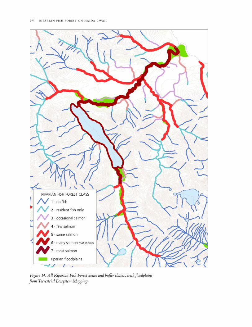
Figure 14. All Riparian Fish Forest zones and buffer classes, with floodplains from Terrestrial Ecosystem Mapping.

35

The final step was to merge the selected floodplain features with the stream-buffered riparian zone network and assign them a fishy-ness index value consistent with the intersecting stream — for example, if a floodplain was drained by a “class 5-some salmon” stream, then that was the fishy-ness value attributed to the floodplain. In those few cases where large floodplains with high fish values include very small tributaries (magnitude 1–4) with lesser fish values, the small streams’ fishyness values are retained.

The result for Mathers Creek on Louise Island is illustrated in Figure 15, which uses the black background we chose to enhance the visibility of the entire stream-RFF complex in the final printed display. Figure 16 shows the same coverage overlaid transparently on a colour orthophoto taken in 2003.

The end result was a single, coherent GIS coverage suitable for comparative analysis with other map layers such as ecological regions and logging history. A 24- by 36-inch colour poster was printed for public distribution (see Figure 17). Digital versions are available at www.spruceroots.org in PDF and Google Earth formats.


Figure 15. Final map theme for printed poster.

37

Figure 16. Final map theme overlaid on an airphoto.


Figure 17. Riparian Fish Forest poster of all Haida Gwaii (24 x 36 inches).

39

Results by ecosections

Scientists have described two major physiographic regions on Haida Gwaii (Brown 1968, Demarchi 1995) and named them the Queen Charlotte Lowland Ecoregion and the Queen Charlotte Ranges Ecoregion — which in turn is comprised of the west coast Windward Queen Charlotte Ranges Ecosection and the central Skidegate Plateau Ecosection. We have taken the editorial liberty of calling the west coast ecosection the Windward Haida Gwaii (see Figure 18).

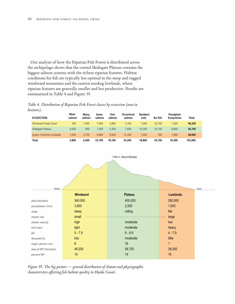
The Queen Charlotte Lowland is an area of low relief in the northeastern part of Haida Gwaii. The weather is cool and wet, with annual precipitation averaging 1,600 mm (63 inches). Glacial sands and gravels and bedrock are generally nutrient-poor. The landscape is dominated by extensive blanket bogs, shallow lakes and scrub forest, interspersed with small patches of productive forest in better drained areas and on richer bedrock. Drainage is generally slow and poor; many streams and lakes are darkly stained by tannin, and are generally acidic (pH 4–7.9) with low dissolved oxygen levels.

Windward Haida Gwaii is a steep, rugged, moutainous terrain of intrusive bedrock and volcanics, subject to the full force of Pacific Ocean weather systems with extreme wind and wave exposure and heavy precipitation, averaging 3,900 mm (154 inches) annually. The Queen Charlotte Ranges are the dominant landform and they descend abruptly to the ocean, forming a rocky coastline drained mostly by short, fast, steep streams that are relatively lightly stained, with slightly higher pH (5–7.9) and dissolved oxygen levels than the Lowland.

The Skidegate Plateau is a rolling peneplain on the leeward side of the Queen Charlotte Ranges, underlain by volcanics and nutrient-rich sedimentary rocks. The average annual precipitation is about 2,500 mm (98 inches), including deep snow in winter at higher elevations. Many streams originate in steep mountain headwaters and gullies, carrying waterborne sediments and organic materials to larger lakes and streams, valley bottom fans and floodplains at lower elevation. In general, stream velocities, pH levels (6–8.9), stain and dissolved oxygen levels are moderate.

Figure 18. Major ecological regions of Haida Gwaii, based on physiography and climate.


Our analysis of how the Riparian Fish Forest is distributed across the archipelago shows that the central Skidegate Plateau contains the biggest salmon systems with the richest riparian features. Habitat conditions for fish are typically less optimal in the steep and rugged windward mountains and the eastern muskeg lowlands, where riparian features are generally smaller and less productive. Results are summarized in Table 4 and Figure 19.

Table 4. Distribution of Riparian Fish Forest classes by ecosection (area in hectares).

area (hectares)

precipitation (mm)

slope

stream size

stream velocity

H2O stain

pH

dissolved O2

major salmon runs

area of RFF (hectares)

percent RFF

400,000

2,500

rolling

moderate

moderate

6 - 8.9

moderate

16

56,700

14

340,000

3,900

steep

small

high

light

5 - 7.9

lots

8

48,200

14

260,000

1,600

flat

large

low

heavy

4 - 7.9

little

1

38,000

16

Windward Plateau Lowlands

West East

1140 m - Mount Moresby

Figure 19. The big picture — general distribution of climate and physiographic characteristics affecting fish habitat quality in Haida Gwaii.

ECOSECTION salmon Most Many

salmon Some salmon salmon

Few Occasionalsalmon

Resident only No fish

Floodplain Ecosystems Total

Windward Haida Gwaii 300 1,900 7,000 3,800 5,300 7,600 20,700 1,600 48,200

Skidegate Plateau 4,500 900 7,300 5,300 7,600 10,200 14,100 6,800 56,700

Queen Charlotte Lowlands 1,000 3,700 8,800 9,000 12,300 1,000 300 1,900 38,000

Total 5,800 6,500 23,100 18,100 25,200 18,800 35,100 10,300 142,900

41

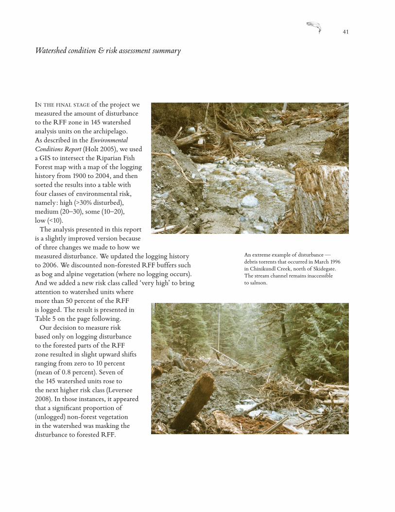
An extreme example of disturbance — debris torrents that occurred in March 1996 in Chinikundl Creek, north of Skidegate. The stream channel remains inaccessible to salmon.

Watershed condition & risk assessment summary

In the final stage of the project we measured the amount of disturbance to the RFF zone in 145 watershed analysis units on the archipelago. As described in the Environmental Conditions Report (Holt 2005), we used a GIS to intersect the Riparian Fish Forest map with a map of the logging history from 1900 to 2004, and then sorted the results into a table with four classes of environmental risk, namely: high (>30% disturbed), medium (20–30), some (10–20), low (<10).

The analysis presented in this report is a slightly improved version because of three changes we made to how we measured disturbance. We updated the logging history to 2006. We discounted non-forested RFF buffers such as bog and alpine vegetation (where no logging occurs). And we added a new risk class called ‘very high’ to bring attention to watershed units where more than 50 percent of the RFF is logged. The result is presented in Table 5 on the page following.

Our decision to measure risk based only on logging disturbance to the forested parts of the RFF zone resulted in slight upward shifts ranging from zero to 10 percent (mean of 0.8 percent). Seven of the 145 watershed units rose to the next higher risk class (Leversee 2008). In those instances, it appeared that a significant proportion of (unlogged) non-forest vegetation in the watershed was masking the disturbance to forested RFF.


Table 5. Logging disturbance and risk assessment of 145 watershed units — based on percentage of forested RFF logged (2006).

Watershed Unit Name Area (ha) Area of RFF (ha)

Forested RFF (ha)

% RFF Forest

Logged Risk Level

Skidegate Lake 16,090 2,876 2,730 88% Very HighAero Camp 4,131 623 603 83% Very HighBuckley Bay 3,100 362 353 81% Very HighTowustasin Hill 4,529 561 533 76% Very HighAlliford Bay 6,807 1,084 1,057 74% Very HighPacofi Bay 3,979 567 555 72% Very HighDeena Creek 7,003 1,633 1,533 70% Very HighBlackwater Creek 3,435 493 488 66% Very HighRenner Pass 4,912 476 419 64% Very HighMamin River 11,057 1,869 1,765 62% Very HighBrent Creek 3,447 503 485 62% Very HighSkidegate Channel 1,651 291 273 59% Very HighCowhoe Bay 2,219 128 125 58% Very HighMosquito Lake 8,689 1,582 1,393 58% Very HighHonna River 4,750 615 601 56% Very HighGold Creek 3,250 531 504 55% Very HighFlorence Creek 5,393 735 722 54% Very HighTalunkwan Island 4,349 641 625 54% Very HighKing Creek 2,287 329 327 54% Very HighMathers Creek 8,411 1,332 1,236 53% Very HighDinan Bay 4,666 534 511 53% Very HighUpper Yakoun River 6,036 1,388 1,312 52% Very HighWaste Creek 3,363 440 430 51% Very HighAtli Bay 8,891 912 903 49% HighSewell Inlet 5,578 793 772 49% HighTangil Penninsula 2,484 409 388 48% HighSkedans Creek 5,189 975 867 48% HighGogit Passage 11,301 1,224 1,195 47% HighSlatechuck Creek 4,923 629 567 46% HighShields Bay 7,006 1,119 877 46% HighBeattie Anchorage 2,995 312 293 46% HighHaans Creek 7,315 905 856 45% HighBegbie Penninsula 5,198 257 256 45% HighNewcombe Inlet 8,784 1,178 1,067 44% HighBotany Inlet 8,225 1,487 1,397 44% HighTrounce Inlet 2,686 423 342 44% HighRockfish Harbour 4,748 456 435 42% HighGray Bay Cumshewa 10,449 1,181 1,095 42% HighMcClinton Bay 6,185 791 754 42% HighLower Yakoun River 12,425 2,609 2,306 39% HighNaden River 12,690 1,905 1,724 37% HighDavidson Creek 11,888 2,037 1,919 37% HighBonanza Creek 4,450 695 671 36% HighGhost Creek 4,863 833 806 35% HighCrescent Inlet 4,067 464 408 34% HighLong Inlet 5,710 884 678 34% HighRoy Lake 4,927 527 478 32% High

43

Lagoon Inlet 3,191 571 524 32% HighSewall Creek 4,965 452 404 29% MediumCanyon Creek 2,724 344 291 29% MediumIan Lake 9,394 1,117 1,086 29% MediumKuper Inlet 9,217 1,263 911 29% MediumThree Mile Creek 2,818 337 330 29% MediumBreaker Bay Creek 2,938 366 336 29% MediumNewcombe Peak 7,255 1,150 1,063 29% MediumTanu 3,634 406 394 28% MediumRiley Creek 3,142 517 496 27% MediumSurvey Creek 5,444 813 796 27% MediumAin River 4,119 790 737 25% MediumAwun River 7,216 806 770 25% MediumStanley Creek 6,128 930 852 24% MediumLawn Hill 7,988 550 476 24% MediumQueen Charlotte Skidegate 6,444 481 440 23% MediumTartu Inlet 6,615 929 811 23% MediumDatlamen Creek 6,179 777 753 22% MediumBoulton Lake 7,679 768 521 20% MediumDawson Harbour 5,464 799 587 16% SomeKumdis Island 3,602 209 159 14% SomeHangover Creek 1,979 284 265 13% SomeLignite Creek 14,720 1,901 1,696 12% SomeDawson Inlet 4,145 659 388 12% SomeCave Creek 10,744 1,781 1,566 11% SomeChaatl Island 3,709 319 285 11% SomeBill Creek 3,496 401 356 11% SomeGregory Creek 3,391 591 559 10% SomeWatun River 8,572 1,169 818 9% LowPhantom Creek 1,894 342 332 9% LowKumdis Creek 6,152 475 415 8% LowSkonun River 15,773 2,681 1,760 8% LowIan Southwest 2,461 278 267 8% LowBill Brown Creek 2,871 374 352 8% LowKitgoro Inlet 8,879 1,058 970 6% LowHibben Island 3,392 436 381 5% LowIan Northeast 5,979 817 689 5% LowGudal Bay 9,403 1,511 1,040 5% LowBurnaby Island 7,410 577 533 5% LowKano Inlet 11,598 1,799 1,515 5% LowMayer Lake 12,661 1,493 1,264 4% LowBlackbear Creek 1,738 267 263 4% LowLower Tlell River 10,398 1,756 1,346 3% LowKlunkwoi Bay 5,114 790 594 3% LowLog Creek 4,929 463 428 3% LowTara Creek 4,547 604 578 3% LowYakoun Lake 8,372 1,428 1,234 3% LowHuston Inlet 9,350 806 726 3% LowKitt Hawn Creek 9,791 1,253 922 2% LowGeike Creek 3,232 231 221 2% LowHaines Creek 11,678 1,846 1,718 2% Low


Forested RFF (ha)

% RFF Forest

Logged Risk Level


Crease Creek 2,337 222 196 1% LowBottle Inlet 7,334 946 745 1% LowSecurity Inlet 7,911 1,280 1,197 1% LowMarshall Inlet 8,209 1,177 1,153 1% LowKootenay Inlet 12,626 1,747 1,409 0% LowFairfax Inlet 4,282 722 611 0% LowHiellen River 14,662 2,168 1,483 0% LowKung 8,621 1,334 1,129 0% LowHancock River 19,976 3,217 2,586 0% LowFeather Creek 4,567 546 482 0% LowSkittagetan Lagoon 11,925 1,450 1,025 0% LowLeila Creek 7,000 805 753 0% LowCraft Bay 5,365 721 656 0% LowGovernment Creek 1,932 314 279 0% LowCape Ball Creek 19,710 2,621 2,178 0% LowAthlow Bay 5,216 793 693 0% LowBeresford Creek 13,421 2,677 2,485 0% LowChristie River 10,907 2,217 1,830 0% LowCoates Creek 8,546 1,474 1,349 0% LowFortier Hill 3,246 394 340 0% LowGowgaia Bay 16,330 1,893 1,636 0% LowHana Koot Creek 6,277 1,116 1,062 0% LowHippa Island 6,470 804 715 0% LowHosu Cove 2,141 158 148 0% LowHoya Passage 2,574 379 316 0% LowInskip Channel 3,003 367 289 0% LowJalun River 18,738 3,493 3,047 0% LowKlashwun Point 4,257 832 694 0% LowKunghit Island 12,905 957 919 0% LowLangara Island 3,188 439 378 0% LowLepas Bay 6,551 945 833 0% LowLouscoone Inlet 6,285 601 551 0% LowMercer Lake 4,036 621 520 0% LowOeanda River 16,640 2,701 1,985 0% LowOtard Creek 9,043 1,682 1,470 0% LowOtun River 14,597 2,521 1,926 0% LowPort Chanal 4,545 802 646 0% LowPuffin Cover 9,685 1,513 1,198 0% LowRose Inlet 10,938 801 705 0% LowRose Spit 6,126 784 436 0% LowSeal Inlet 10,229 1,480 1,247 0% LowSialun Creek 8,439 1,392 1,281 0% LowSkaat Harbour 6,043 583 535 0% LowStaki Bay 6,469 693 578 0% LowSunday Inlet 8,617 1,472 971 0% LowTian Head 4,987 679 606 0% LowWia Point 6,720 1,051 783 0% Low


Forested RFF (ha)

% RFF Forest

Logged Risk Level

45

Figure 20. Watershed risk assessment — indicating the risk that forest conditions important to healthy fish populations have been damaged or destroyed. Based on Table 5.


The Environmental Conditions Report also used salmon as an indicator species and examined escapement data for a 50-year period. Holt (2005) concluded that although many of the data are unsystematic, there have been clear declines in fish abundance in local streams and many of these can be correlated with degradation of fish habitat caused by logging and road building (Riddell 2004).

For this report we examined disturbance in the top ten salmon producing streams as identified in the RFF model as Class 7 – Most Salmon. A total of 34 watershed units are associated with the top ten salmon streams and half of them are at high or very high risk (see Table 6).

Table 6. Risk levels in watersheds associated with the top ten salmon streams.

Watershed Risk Level Skidegate Lake Very HighDeena Creek Very HighMamin River Very HighBrent Creek Very HighMosquito Lake Very HighGold Creek Very HighKing Creek Very HighMathers Creek Very HighUpper Yakoun River Very HighSkedans Creek High Gogit Passage High Slatechuck Creek High Lower Yakoun River High Naden River High Davidson Creek High Ghost Creek High Long Inlet High Lagoon Inlet High Canyon Creek Medium Three Mile Creek Medium Survey Creek Medium Ain River Medium Awun River Medium Lignite Creek Some Phantom Creek Low Kitgoro Inlet Low Lower Tlell River Low Klunkwoi Bay Low Fairfax Inlet Low Feather Creek Low Leila Creek Low Athlow Bay Low Jalun River Low Mercer Lake Low

47

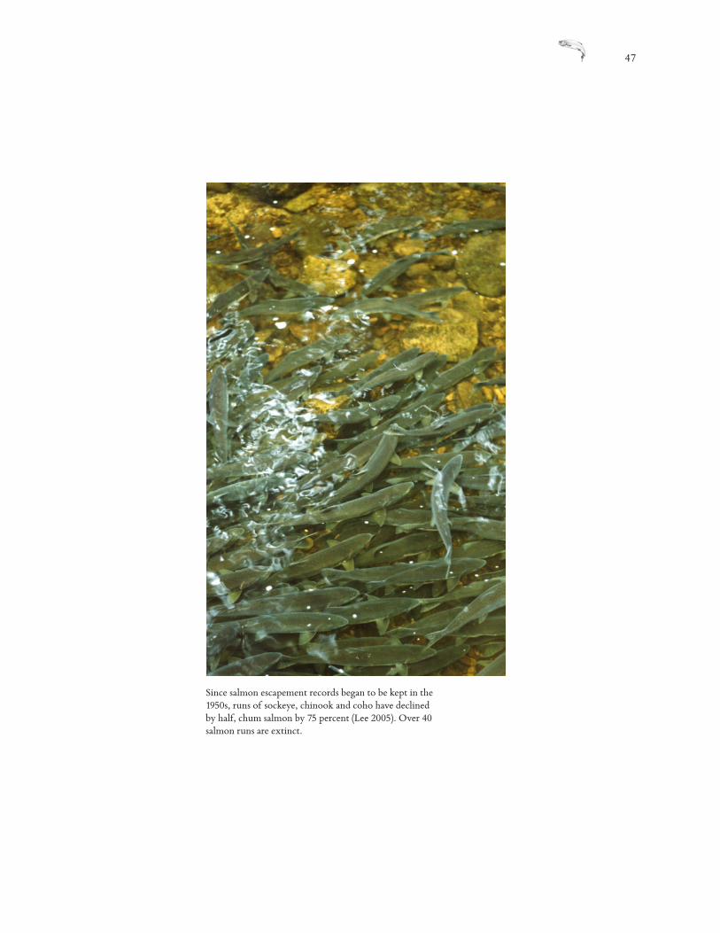
Since salmon escapement records began to be kept in the 1950s, runs of sockeye, chinook and coho have declined by half, chum salmon by 75 percent (Lee 2005). Over 40 salmon runs are extinct.


References

Broadhead, J. and D. Leversee. 2004. Logging Haida Gwaii 1901–2004 (map animation). Gowgaia Institute. Queen Charlotte, BC. http://www.spruceroots.org/LogVideo/LogVid.html

Brown, A.S. 1968. Geology of the Queen Charlotte Islands, British Columbia. Bulletin 54, BC Department and Petroleum Resources, Victoria, BC.

Clement, Chris. 2004. Personal Communication. Victoria, BC.

Clement, Chris. 1995. Ecosystem Units of Louise Island, Chadsey Creek and Haans Creek. Shearwater Mapping Ltd. Victoria, BC.

Cober, A. 2004, 2005. Personal Communication. Queen Charlotte, BC.

Council of the Haida Nation (CHN) 2004. Haida Land Use Vision (HLUV) — Haida Gwaii Yah’guudang (respect for this place) in Haida Gwaii Land Use Plan 2006. http://ilmbwww.gov.bc.ca/lup/lrmp/coast/qci/docs/HLUVpublic.pdf

Dalzell, K.E. 1973. The Queen Charlotte Islands, Vol. 2, Places and Names. Harbour Publishing, Madiera Park, BC.

Demarchi, D.A. 1995. Ecoregions of British Columbia (4th ed.). B.C. Ministry of Environment, Victoria, BC.

Farrell, G. 2004, 2005. Personal Communication. Queen Charlotte, BC. Gomi, T, R. Sidle and J. Richardson. 2002. Understanding Processes and Downstream Linkages of Headwater Systems. BioScience 52: 905-916

Green, R. and K. Klinka. 1994. A Field Guide to Site Identification and Interpreta tion for the Vancouver Forest Region. British Columbia Ministry of Forests, Vancou ver, BC.

Holt, R. 2005. Environmental Conditions Report for the Haida Gwaii / Queen Charlotte Islands Land Use Plan. BC Integrated Land Management Branch.

Victoria, BC. http://ilmbwww.gov.bc.ca/lup/lrmp/coast/qci/hgqci_env.htm

Hyatt, J. 2005. Personal Communication. Lawn Hill, BC.

CRGB Crown Registry and Geographic Base 1997, 2003. Orthophotos of the Queen Charlotte Islands. Integrated Land Management Bureau. Victoria, BC.

Katinic, P. 2004, 2005. Personal Communication. Skidegate, BC.

Lee, L. 2001. Reconnaissance Report (1:20,000) Fish and Fish Habitat Inventory for the Timber Supply Area (TSA), Naikoon Park and private land portion of the Tlell River Watershed. Tlell Watershed Society, Tlell, BC.

Lee, L. 2004, 2005. Personal Communication. Salmon abundance trends based on SED. Tlell, BC.

49

Leversee, D. 2008. Calculation of Watershed Condition by Logging Disturbance to Forested RFF. Spreadsheet <filename: RFF_HVFH_PTT_Stats.xls> distributed to agencies involved in SLUA implementation. Gowgaia Institute, Queen Charlotte, BC.

Lewis, Terence 1981. The Ecosystems of Block 18 of Tree Farm License 2, Queen Charlotte Islands, BC. 82 p.

Lewis, Terence 2003. The Ecosystems of Block 6, Tree-Farm Licence 25, Queen Charlotte Islands, BC. Prepared For Western Forest Products, Inc. May 2003 (Second Edition).

Ministry of Energy, Mines and Petroleum Resources 2004. Digital Elevation Model of the Queen Charlotte Islands, 25m resolution. By Yao Cui, BC Geological Survey Branch, Victoria, BC.

Ministry of Environment 1995-2004. Ecosystem Units of Tree Farm License 39, Block 6; and, portions of the Haida Gwaii TSA, in Terrestrial Ecosystem Mapping Home. Victoria, BC. http://www.env.gov.bc.ca/ecology/tem/index.html

Ministry of Forests 1995. Forest Practices Code of British Columbia – Riparian Management Area Guidebook. http://www.for.gov.bc.ca/tasb/legsregs/fpc/fpcguide/riparian/Rip-toc.htm

Moore, K. 2005. Personal Communication. Queen Charlotte, BC.

Mount, C. 2000. Post Layout Terrain Stability Assessment: Proposed Road - Taxus Mainline (Stn. 0+000 - 2+670) Report. Coast Forest Management Ltd., Campbell River, BC.

Naiman, R., R. Bilby, and P. Bisson. 2000. Riparian Ecology and Management in the Pacific Coastal Rainforest. Bioscience. 50(11):996-1011.

Northcote, T.G., A.E. Peden, & T.E. Reimchen. 1989. Fishes of the Coastal Marine, Riverine and Lacustrine Waters of the Queen Charlotte Islands, in The Outer Shores edited by G. Scudder & N. Gessler. Skidegate, BC: Queen Charlote Islands Museum Press.

Pojar, J. 1999. Personnel Communication. Tlell River Watershed Local Resource Use Plan process. Tlell, BC.

Price, K. and D. McLennan. 2001. Hydroriparian Ecosystems of the North Coast: Riparian Background Report to North Coast LRMP. Province of British Columbia. Victoria, BC.

Reimchen, T.E. 1992. Naikoon Provincial Park Queen Charlotte Islands/Haida Gwaii Natural History and Biophysical Data for Freshwater Habitats. [Report] Islands Ecological Research. Queen Charlotte, BC.

Reimchen, T.E. 2004. Marine and Terrestrial Ecosystem Linkages: The Major Role Of Salmon and Bears in Riparian Communities, in Botanical Electronic News, ISSN 1188-603X http://www.ou.edu/cas/botany-micro/ben/ben328.html


Reimchen, T.E. 2006. Personal Communication. Victoria, BC.

Riddell, B. 2004. Pacific Salmon Resources in Central and North Coast British Co lumbia. Pacific Fisheries Resource Conservation Council (PFRCC).

Reindl, F. 2005. Personal Communication. Port Clements, BC.

Vigneault, L. 2004, 2006. Personal Communication. Tlell, BC.

Walsh, M. 2005. Personal Communication. Queen Charlotte, BC.

Data sources

Bartier, P. 1994. Gwaii Haanas Biophysical Surveys of Freshwater Aquatic Habitat. Parks Canada, Queen Charlotte.

BC Fisheries, 2000. Fisheries Information Summary System. Database. Aquatic Information Branch Fisheries Information, Victoria. http://www.bcfisheries.gov.bc.ca/fishinv/fiss.html

Bocking, R., K. Rood, R. Jones, and S. Yazvenko. 1997. Overview Assessment of Stream and Riparian Habitat of Louise Island Streams [Report]. LGL Limited Envi-ronmental Research Associates, Sidney.

Department of Fisheries and Oceans, BC Fisheries. 2000. The Fisheries Information Summary System. Database. Aquatic Information Branch Fisheries Information, Victoria. Last accessed December 2000.

Farrell, George. 2004. Personnel Communication. Queen Charlotte.

Ferguson, J.P., M. Gaboury, and R.C. Bocking, 2000. Bonanza and Gregory Creek Watershed Level 1 Fish Habitat Assessments [Report]. LGL Limited Environmental Research Associates, Sidney.

Ferguson, J.P. and R.C. Bocking, 1999. Mathers Creek Watershed Level 1 Fish Habi tat Assessments [Report]. LGL Limited Environmental Research Associates, Sidney.

Ferguson, J.P. and R.C. Bocking, 1999. Rennell Sound Watersheds Level 1 Fish Habitat Assessments [Report]. LGL Limited Environmental Research Associates, Sidney.

Ferguson, J.P. and R.C. Bocking, 1997. Watershed Restoration Program Level 1 Stream and Riparian Skedans Watershed Rehabilitation [Report]. LGL Limited Environmental Research Associates, Sidney.

51

Fisheries and Oceans Canada, 1990. Fish Habitat Inventory and Information Program. Stream Summary Cata logue. Vancouver.

Forest Renewal British Columbia (FRBC) 1999. Fish and Fish Habitat Inventory for Security Creek [Report]. FDIS 717396.

Jacobson, T. 1999. Coates Creek Reconnaissance (1:20,000) Fish and Fish Habitat Assessment [Report]. Salmon Unlimited Society, Queen Charlotte.

Karanka, E.J. 1986. Davidson Creek Inventory Project Report. Department of Fish-eries and Oceans Canada. Queen Charlotte.

Lee, L. 2001. SBFEP Stream Classification Report for Proposed Cutblock Area 76A, West Massett Inlet. MTE Inc. Tlell.

Lee, L. 2000. Stream Classification Report for SBFEP Cutblocks A58446 and A58447. MTE Inc. Tlell.

Lee, L. 1999. Stream Classification Report for Cutblock Awun 44. MTE Inc. Tlell.

Lee, L. 1998. SBFEP Stream Classification Report for TSA42720, TSA54789H and TSA58328. MTE Inc. Tlell.

Lee, L. and L. Vigneault. 2002. SBFEP Stream Classification Assignments 1-5. [Re-port Series]. MTE Inc. Tlell.

Moore, K. 1992. Non-Timber Resource Values in the Kootenay Inlet Development Area - Assessment and Recommendations. [Report] Moore Resource Management. Queen Charlotte.

Mount, C. 2000. Post Layout Terrain Stability Assessment: Proposed Road - Taxus Mainline (Stn. 0+000 - 2+670) Report. Coast Forest Management Ltd. Campbell River.

Vigneault, L. 2003. Personal Communication. Tlell.

Vigneault, L. 1998. SBFEP Pure Lake Road and Block Layout for Cutblocks A58367 and A58370 [Report]. MTE Inc. Tlell.

Vigneault, L. 1996. Stream classification for upper Gregory Creek [Report]. Bar Environmental. Tlell.

Weyerhaeuser Canada Ltd. 2003. Weyerhaeuser Cutblock Silviculture Perscriptions 1995-2003 [Files]. Weyerhaeuser, Juskatla.

a portrait of freshwater fish distribution iparian forests ...€¦ · riparian fish forest on...

Documents