HAL Id: hal-02377794https://hal.archives-ouvertes.fr/hal-02377794

Submitted on 3 Jan 2021

HAL is a multi-disciplinary open accessarchive for the deposit and dissemination of sci-entific research documents, whether they are pub-lished or not. The documents may come fromteaching and research institutions in France orabroad, or from public or private research centers.

L’archive ouverte pluridisciplinaire HAL, estdestinée au dépôt et à la diffusion de documentsscientifiques de niveau recherche, publiés ou non,émanant des établissements d’enseignement et derecherche français ou étrangers, des laboratoirespublics ou privés.

A partitioned two-step solution algorithm for concurrentfluid flow and stress–strain numerical simulation in

solidification processesShaojie Zhang, Gildas Guillemot, Charles-André Gandin, Michel Bellet

To cite this version:Shaojie Zhang, Gildas Guillemot, Charles-André Gandin, Michel Bellet. A partitioned two-step so-lution algorithm for concurrent fluid flow and stress–strain numerical simulation in solidification pro-cesses. Computer Methods in Applied Mechanics and Engineering, Elsevier, 2019, 356, pp.294-324.�10.1016/j.cma.2019.07.006�. �hal-02377794�

1

A partitioned two-step solution algorithm for concurrent fluid flow and stress-strain numerical simulation in

solidification processes

Shaojie Zhang, Gildas Guillemot, Charles-André Gandin and Michel Bellet*

MINES ParisTech, PSL Research University, CEMEF - Centre de Mise en Forme des Matériaux, CNRS UMR

7635, CS 10207, 1 rue Claude Daunesse, 06904 Sophia Antipolis cedex, France

Abstract: One of the critical challenges encountered when modeling solidification processes is to

achieve a concurrent and efficient computation of fluid flow and solid mechanics. Several detrimental

casting defects justify this development: cracks, either as a result of stresses built at surface or sub-

surface in solidified regions during the filling stage of ingot casting, or due to hot tears deep in the mushy

zone during solidification; macrosegregation, as a result of thermo-solutal convection flows and possible

deformation of solid. It is therefore of crucial importance to provide for a global and synthetic analysis

of casting processes considering a single numerical modelling that includes coupling between fluid flow

and solid mechanics. A two-step solution strategy combining fluid flow and solid mechanics has been

developed. A partitioned formulation is used, performing at each time increment, separately a solid-

oriented resolution and a fluid-oriented resolution. Liquid flow (natural convection or forced flow during

ingot filling stage), solidification shrinkage as well as thermally induced deformation of the solid regions

are taken into account. The paper presents the numerical formulation in a level set finite element context,

and associated validation tests. Application in a practical case corresponding to an ingot filling is

proposed in order to investigate the solidification process and associated fluid flow and stress evolutions.

Some discussions on computations time and others numerical aspects are also developed at the end in

order to show the potential improvements of this methodology.

Key words: Solidification; Solid-fluid interaction; Thermohydraulics; Thermomechanics; Finite element; Level

set

*Corresponding author. Tel.: +33 4 93 95 74 61, michel.bellet@mines-paristech.fr.

Email addresses: shaojie.zhang@mines-paristech.fr (S. ZHANG), gildas.guillemot@mines-paristech.fr (G.

Guillemot), charles-andre.gandin@mines-paristech.fr (Ch.-A. Gandin), michel.bellet@mines-paristech.fr (M.

Bellet).

2

1 Introduction

In industry, it is of crucial importance to predict fluid flow induced segregation phenomena in ingot

castings. Concurrently, deformation related defects such as hot tears in the mushy zone or surface

cracking during cooling need prediction of stresses built upon cooling. Modelling mechanical problems

in the context of solidification thus requires solving both liquid flow in the non-solidified regions and

solid deformation in solidified regions.

The liquid flow, carrying heat and chemical species, determines the temperature field and segregation

patterns and hence influences the solidification path and the deformation induced by thermal dilatation

and non-uniform cooling. In large ingot casting, a considerable amount of the ingot volume may solidify

during the filling stage due to long filling duration, leading to formation of surface or sub-surface cracks.

Similar observation is possible in continuous casting: surface cracks appear in the thin solid shell formed

in the mold region where an intense fluid flow is induced by nozzle jet. Therefore an efficient mechanical

analysis through numerical simulation should consider concurrently stress and strains development in

the solid regions, and flow evolution in the fluid regions.

Nowadays, either the simulation of fluid flow during ingot filling or the simulation of deformation and

stress during cooling are routinely performed by software dedicated to the modelling of casting

processes. Computational fluid dynamics (CFD) codes, based on Navier-Stokes equations, and

including turbulence models, are efficient to model liquid flow. But such software does not provide

access to stress and strain evolution in the solidified domains. Conversely, structural thermomechanical

codes, assuming an elasto-viscoplastic behavior, fail in modelling the fluid related phenomena. However,

few propositions have emerged for concurrent simulation of fluid related phenomena and stress/strain

analysis.

Numerical methods for the solution of such fluid-structure interaction (FSI) can be classified in two

categories: the monolithic approach and the partitioned approach. In a monolithic approach, a single set

of momentum and mass conservation equations is solved in the whole domain encompassing the fluid

and the solid regions. In a partitioned formulation, separate fluid and solid problems are solved and

coupled. In order to estimate the coupling effect, Heil et al. [1] have defined a FSI index 𝑄, as the ratio

of the flow stresses in the fluid and solid (or structure) regions: 𝑄 = �̅�𝑓𝑙𝑢𝑖𝑑 �̅�𝑠𝑜𝑙𝑖𝑑⁄ , where �̅� stands for

the equivalent von Mises stress. In the context of solidification, the FSI index keeps very low values.

The highest 𝑄 values are encountered for thin solid shells just below the solidus, when exposed to fluid

flow, or in mushy zones just above the solidus. In such cases, the liquid dynamic viscosity 𝜇𝑙 is about 10−3 Pa ⋅ s. Assuming a generalized strain rate 𝜀̅̇ in the metal flow in the range of 10 to 1000 s−1, �̅�𝑓𝑙𝑢𝑖𝑑, being equal to 3𝜇𝑙𝜀̅̇, is of the order of 10−2 to 1 Pa. The flow stress �̅�𝑠𝑜𝑙𝑖𝑑 of the solid zone at

very high temperature being about 1 to 10 MPa, the FSI index 𝑄 is then found in the range [10−9, 10−6], expressing a very weak interaction. More concretely, such a solid region is hardly deformed by fluid

flow. It was proved by [1] that for such a weak FSI problem, a partitioned approach is more efficient

than a monolithic one. Actually, such a low 𝑄-value problem is associated with very poor conditioning

3

of the stiffness matrices arising in the solution of the momentum conservation. That explains why the

liquid viscosity should be arbitrarily maintained at a high value when considering simultaneously liquid

and solid metal in a single-step solution of a mechanical problem [2].

As a consequence, in the present work, a partitioned two-step solution algorithm is developed for

application to the modeling of solidification processes in ingot casting. The momentum and mass

conservations are solved twice at each time increment, thus defining the two steps. In the first step, a

solid-oriented solution deriving from an existing thermomechanical solidification model [2,3] is

performed in order to calculate stress and deformation fields in solid containing regions. In the second

step, a liquid-oriented solution is derived, which addresses the fluid flow in the bulk liquid and in the

mushy zone while making use of the solid velocity field derived from the first step. Volume averaging

and Darcy’s law are used to model the interactions between solid and liquid phases in the mushy zone.

Both solutions are formulated with the finite element (FE) method on a single three-dimensional (3D)

spatial domain which includes the metal and a surrounding gas as sub-domains. The level set method is

used to track the motion of the metal/gas boundary induced by hydrodynamics, solidification shrinkage,

thermal dilatation and deformation phenomena. The algorithm is coupled with an existing non-linear

energy solver to calculate the temperature field [4]. Validation is demonstrated by comparison with

analytical solutions in the context of directional solidification. Finally, application to case studies similar

to industrial solidification processes (ingot filling and cooling) is presented and discussed.

2 Numerical model

Typical regions found in casting processing are shown in Fig. 1a, except the molds that are not described

in the present contribution. The numerical model of the partitioned solution algorithm consists

principally of two steps: the first one, labeled STEP I, is a solid-oriented solution of the momentum and

mass conservation equations, dedicated to the strain and stress computation in the regions partially or

completely solidified. The second one, labeled STEP II, is a fluid-oriented solution of the momentum

and mass conservation equations that aims at determining velocity and pressure fields in the fluid-

containing zones, i.e. regions with liquid, mushy zone and gas. In this paper, the presentation will be

focused on the numerical issues associated with STEP I and STEP II and with their organization as

sequential solvers. The bases of the numerical solutions developed to solve the heat transfer problem

and the mechanical problem will not be detailed hereafter. Details can be found in [2-4]. In the following,

the level set method is first presented in Section 2.1 as it provides the relevant framework to formulate

a unique set of conservation and constitutive equations for the whole domain (i.e. metal and surrounding

gas) as well as to track the metal/gas interface between the two sub-domains during the casting process.

Conservation and constitutive equations in each region and the final formulation in the level set

framework will be described in Section 2.2 for the solid-oriented solution and in Section 2.3 for the

liquid-oriented solution. Section 2.4 will be devoted to the general presentation of the partitioned two-

step solution algorithm.

4

2.1 Level set method

The level set method was initially introduced by Osher and Sethian [5] in order to follow moving

interfaces. This method has been largely applied to model dynamic interface problems in computational

fluid mechanics [6,7] because of its facility to handle topological changes and geometrical dependent

quantities. In the present study, the interface 𝛤 between the metal and gas sub-domains, respectively 𝛺𝑀and 𝛺𝐺 , is implicitly represented by the zero-value of a signed distance function, also called level

set function, 𝜑(𝒙, 𝑡) for any given point 𝒙 of a global domain 𝛺 and time 𝑡 as :

𝜑(𝒙, 𝑡) = {𝑑(𝒙, 𝑡) if 𝒙 ∈ 𝛺𝑀0 if 𝒙 ∈ 𝛤−𝑑(𝒙, 𝑡) if 𝒙 ∈ 𝛺𝐺 (1)

where 𝑑(𝒙, 𝑡) denotes the geometric distance from point 𝒙 to the interface 𝛤 at time 𝑡. In the Eulerian

context, this level set function is convected by the solution velocity field 𝒗 through the following

transport equation: 𝜕𝜑𝜕𝑡 + 𝒗 ∙ ∇𝜑 = 0 (2)

However, the eikonal property (i.e. unitary gradient vector) of the level set function is generally not

preserved after such a transport. This may be problematic when special meshing technique at interface

depends on the geometrical distance, or when the interface motion is curvature dependent through

surface tension. Thus, a reset method developed by Shakoor et al. [8] is used to preserve this property.

The method is based on a geometrical computation of the distance between each FE node and the

convected zero-level set interface. This reset step is performed systematically after each transportation

of the level set function.

Besides, the level set is used to mix material properties in a transition zone around the interface. The

smoothed Heaviside function, ℋ𝑀, is then introduced to indicate locally the type of domain. A smooth

transition over an artificial interface thickness [−𝜀,+𝜀] centered at the zero-level set interface is also

introduced in order to develop a continuous transition between domains. This function is consequently

defined as follows:

ℋ𝑀(𝜑) = { 0 if 𝜑 < −𝜀 1 if 𝜑 > 𝜀 12 (1 + 𝜑𝜀 + 1𝜋 𝑠𝑖𝑛 (𝜋𝜑𝜀 )) if − 𝜀 ≤ 𝜑 ≤ ε (3)

Eq. (3) is used to preserve a smooth transition of physical quantities at interface with an arithmetic

mixing law. Denoting 𝜓𝑀 and 𝜓𝐺 the values of a physical variable 𝜓 relative to sub-domains 𝛺𝑀 and 𝛺𝐺 , the mixed value of 𝜓 through the level set transition zone, �̂�, is defined by: �̂� = ℋ𝑀𝜓𝑀 + (1 −ℋ𝑀)𝜓𝐺 (4)

5

Note that expression (4) holds as well in each of the two sub-domains 𝛺𝑀 and 𝛺𝐺 , i.e. outside of the

transition zone. In the rest of the paper, the level set framework will be used to follow the interface

between metal and gas, as illustrated in Fig. 1b, and the following convention will be used: 𝜑 will be

counted positively in the metal sub-domain (𝛺𝑀), and negatively in gas (𝛺𝐺), so that at any instant ℋ𝑀(𝜑) = 1 for a position 𝒙 in metal, and ℋ𝑀(𝜑) = 0 in gas.

2.2 STEP I: solid-oriented resolution

This section focuses on the evaluation of thermal stresses and strains in the solid zone. The solver used

in STEP I is derived from a previous thermomechanical solidification solver [2,3]. As illustrated in Fig.

1c, two types of constitutive equations are used simultaneously depending on the local state of the metal:

- thermo-elasto-viscoplastic (TEVP) constitutive model in metallic regions where temperature is

lower than a critical temperature, 𝑇𝐶. In the present study, it is supposed that 𝑇𝐶 is lower than

the solidus temperature, 𝑇𝑆.

- thermo-viscoplastic (TVP) model in all other regions (i.e. metallic regions over 𝑇𝐶 as well as

the gas sub-domain).

In the metal sub-domain, the standard Heaviside function, taken for the temperature difference (𝑇𝐶 −𝑇), is introduced as an indicator relative to the use of the TEVP constitutive model. This function

consequently differs from the smoothed Heaviside function, ℋ𝑀, previously introduced. Its value is one

if the temperature is below the critical temperature 𝑇𝐶, and zero otherwise:

𝐻(𝑇𝐶 − 𝑇) = { 0 if 𝑇 > 𝑇𝐶 1 if 𝑇𝑇𝐶 . (5)

Note that depending on the local nature of the material (gas or metal) and on temperature, the TVP

model is either purely Newtonian (gas domain and liquid metal) or viscoplastic (mushy and solid metals

over 𝑇𝐶). If the critical temperature, 𝑇𝐶, is lower than the solidus temperature, 𝑇𝑆, the pure viscoplastic

model is extended to the solid metal. Then elasticity and strain-hardening effects are ignored in the solid

state, between 𝑇𝐶 and 𝑇𝑆, i.e. at high temperature. In the present study, 𝑇𝐶 is taken equal to the solidus

temperature 𝑇𝑆 of the alloy. Thus, metal solid regions are fully modelled with the TEVP model. Both

TVP and TEVP constitutive models are detailed hereunder. Then the associated conservation equations

used with the level set method are introduced. A summary of the weak formulation and its finite element

discretization form is finally provided.

2.2.1 Constitutive models for STEP I

2.2.1.1 Thermo-elasto-viscoplasticity (TEVP): solid metal region

A thermo-elasto-viscoplastic model is relevant below the critical temperature 𝑇𝐶 as mentioned

previously. It is described by the following equations [2]:

6

�̇� = �̇�𝑒𝑙 + �̇�𝑣𝑝 + �̇�𝑡ℎ (6)

�̇�𝑒𝑙 = 𝐄−1�̇� = 1 + 𝜐𝐸 �̇� − 𝜐𝐸 tr(�̇�)𝐈 (7)

�̇�𝑣𝑝 = √32�̅� [�̅� − 𝜎𝑌√3𝐾𝜀̅𝑛]+1𝑚 𝒔 (8)

�̇�𝑡ℎ = − 13𝜌 𝑑𝜌𝑑𝑡 𝐈 (9)

The strain rate tensor �̇� is split into an elastic part, �̇�𝑒𝑙, a viscoplastic part, �̇�𝑣𝑝, and a thermal part, �̇�𝑡ℎ (Eq. (6)). The latter consists of the thermal expansion rate (Eq. (9)), with 𝜌 the density. Eq. (7) yields

the hypoelastic Hooke’s law where E represents the elastic tensor depending on the Young’s modulus E, and the Poisson’s coefficient 𝜐. �̇� denotes the total time derivative of the stress tensor. Eq. (8) gives

the relation between the viscoplastic strain rate and the stress deviator 𝒔. It is reminded here that the

stress deviator is defined as 𝒔 = 𝝈 − 1 3⁄ tr(𝝈)𝐈 = 𝝈 + 𝑝𝐈, where 𝝈 is the Cauchy stress tensor, 𝑝 is the

hydrostatic pressure, and 𝐈 is the identity tensor. Coefficient 𝐾 is the viscoplastic consistency, 𝜎𝑌

denotes the static yield stress below which no viscoplastic deformation occurs. The function [𝑥]+ is

equal to 0 when 𝑥 is negative and to the value 𝑥 otherwise. Coefficients 𝑚 and 𝑛 denote the strain-rate

sensitivity coefficient, and the strain hardening coefficient, respectively. Finally, the corresponding

relationship between the von Mises equivalent stress, �̅� , the generalized plastic strain, 𝜀 ̅, and the

equivalent strain rate, 𝜀̅̇, is given by: �̅� = 𝜎𝑌 +𝐾(√3)𝑚+1𝜀̅̇𝑚𝜀̅𝑛 (10)

2.2.1.2 Thermo-viscoplasticity (TVP): mushy and liquid metal regions, and gas sub-

domain

The thermo-viscoplastic model is used to model the mechanical behavior of gas, liquid and mushy

regions. Possibly this model may be extended to solid metal over 𝑇𝐶. In this case, the compressibility is

only due to the thermal contribution as elasticity is neglected. Equations of the constitutive model are

written as follows: �̇� = �̇�𝑣𝑝 + �̇�𝑡ℎ (11)

�̇�𝑣𝑝 = 12𝐾 (√3𝜀̅̇)1−𝑚𝒔 (12)

�̇�𝑡ℎ = − 13𝜌𝑑𝜌𝑑𝑡 𝐈 (13)

The strain rate tensor �̇� is split into a viscoplastic part, �̇�𝑣𝑝, and a thermal part, �̇�𝑡ℎ (Eq. (11)). Eq. (12)

is the classical constitutive law for a generalized non-Newtonian fluid behavior. It relates the

viscoplastic strain rate �̇�𝑣𝑝 to the stress deviator 𝒔, in which the strain-rate sensitivity 𝑚 continuously

7

increases with the liquid fraction in the mushy zone. The Newtonian behavior, which is assumed to be

the behavior law of the gas and of the liquid metal above its liquidus temperature, 𝑇𝐿, is obtained for 𝑚 = 1. In this case, the viscoplastic consistency 𝐾 is simply the dynamic viscosity of the fluid (liquid

metal or gas). Finally, the corresponding relationship between the von Mises equivalent stress �̅� and the

equivalent strain rate 𝜀̅̇ is the following one: �̅� = 𝐾(√3)𝑚+1𝜀̅̇𝑚 (14)

It is important to note that gas and liquid metal viscosities will be arbitrarily augmented in the present

resolution STEP I, in order to preserve an acceptable conditioning of stiffness matrices (cf analysis in

the Introduction section). As a consequence, the velocity field 𝒗𝐼 will show mitigated values in gas and

liquid metal. However, as it will be seen later, the resolution STEP II will act as a corrector step in order

to finally obtain a good prediction of liquid metal and gas flows.

Mechanical coherency point and continuity with the solid behavior

As reported by Dantzig and Rappaz [9], the mechanical response of the mushy metal is quite different

below and over a critical point named coherency point, which can be characterized by a critical liquid

fraction 𝑔𝑐𝑜ℎ𝑙 . At low volume fractions of liquid (𝑔𝑙 < 𝑔𝑐𝑜ℎ𝑙 ), the mushy metal can be considered as

homogeneous, but simply weakened by the presence of isolated liquid pockets and localized

interdendritic films. Referring to the experimental studies conducted by Vicente-Hernandez [10] using

needle indentation tests of mushy metal, there is a linear variation of both the viscoplastic consistency

and the strain-rate sensitivity between solidus and coherency points: for 𝑔𝑙 ∈ [0, 𝑔𝑐𝑜ℎ𝑙 ], 𝐾(𝑔𝑙) = 𝐾(𝑇𝑆) + 𝜕𝐾𝜕𝑔𝑙 𝑔𝑙 and 𝑚(𝑔𝑙) = 𝑚(𝑇𝑆) + 𝜕𝑚𝜕𝑔𝑙 𝑔𝑙 (15)

with 𝜕𝐾 𝜕𝑔𝑙⁄ < 0 and 𝜕𝑚 𝜕𝑔𝑙⁄ > 0. Using those relations, the continuity with the solid behavior is

ensured, provided that, in the TEVP model, both the yield stress 𝜎𝑌 and the strain hardening coefficient 𝑛 tend to zero at the solidus temperature: see Eqs. (10) and (14).

At higher volume fractions of liquid (𝑔𝑙 ≥ 𝑔𝑐𝑜ℎ𝑙 ), the present model simply expresses a smooth

transition towards the Newtonian behavior characterizing the liquid metal. It consists of a mixture rule

applied to the flow stress. Considering that the flow stress varies by several orders of magnitude between

coherency and liquidus points, a logarithmic mixture rule is proposed:

for 𝑔𝑙 ∈ [𝑔𝑐𝑜ℎ𝑙 , 1], ln (�̅�(𝑔𝑙 , 𝜀 ̅̇)) = ln (�̅�(𝑔𝑐𝑜ℎ𝑙 , 𝜀 ̅̇)) + (ln(�̅�(1, 𝜀̅̇)) − ln (�̅�(𝑔𝑐𝑜ℎ𝑙 , 𝜀 ̅̇))) 𝑔𝑙−𝑔𝑐𝑜ℎ𝑙1−𝑔𝑐𝑜ℎ𝑙

= ln (�̅�(𝑔𝑐𝑜ℎ𝑙 , 𝜀 ̅̇)) 1−𝑔𝑙1−𝑔𝑐𝑜ℎ𝑙 + ln(�̅�(1, 𝜀̅̇)) 𝑔𝑙−𝑔𝑐𝑜ℎ𝑙1−𝑔𝑐𝑜ℎ𝑙

(16)

Expressing then the equivalent stress by Eq. (14), a few additional calculations lead to the expressions

of 𝐾 and 𝑚 as functions of the liquid fraction in the interval of interest:

8

ln𝐾(𝑔𝑙) = ln𝐾(𝑔𝑐𝑜ℎ𝑙 ) + (ln𝐾(1) − ln𝐾(𝑔𝑐𝑜ℎ𝑙 )) 𝑔𝑙 − 𝑔𝑐𝑜ℎ𝑙1 − 𝑔𝑐𝑜ℎ𝑙 (17)

𝑚(𝑔𝑙) = 𝑚(𝑔𝑐𝑜ℎ𝑙 ) + (1 −𝑚(𝑔𝑐𝑜ℎ𝑙 ))𝑔𝑙 − 𝑔𝑐𝑜ℎ𝑙1 − 𝑔𝑐𝑜ℎ𝑙 (18)

2.2.2 Treatment of thermal dilatation and solidification shrinkage in the metal sub-

domain for STEP I

Unlike the metal density 𝜌 in Eq. (9), the metal density in Eq. (13) involves at the same time the effect

of thermal dilatation and solidification shrinkage. In previous works [2,3,11,12], the metal density used

in the solidification interval in Eq. (13) was the mixed density defined by 𝜌 = (1 − 𝑔𝑙)𝜌𝑆 + 𝑔𝑙𝜌𝐿 (19)

where 𝜌𝑆 and 𝜌𝐿 are the metal densities at solidus and liquidus temperatures, respectively. Outside the

solidification interval, [𝑇𝑆, 𝑇𝐿] , the density in fully solid and fully liquid regions is temperature

dependent, respectively corresponding to the function 𝜌𝑠(𝑇) and 𝜌𝑙(𝑇)and thus accounting for thermal

dilatation. Considering Eq. (19), Eq. (13) includes the thermal expansion of the two phases, as well as

the solidification shrinkage in the solidification interval. However, two reasons explain the need to

change expression (19) in the present study:

• Firstly, applying the shrinkage contribution on the whole solidification interval is not appropriate.

This is especially true below the coherency point, in the interval [0, 𝑔𝑐𝑜ℎ𝑙 ], where the stiffness is still

high as it consists of a direct extension of the solid behavior. Applying Eq. (19) would make the

mechanical problem very stiff, initiating possible numerical difficulties and/or giving birth to

spurious local velocity fields.

• Secondly, in the framework of the present two-step solver, we are essentially interested in the

intrinsic velocity of the solid phase (i.e. the movement of the columnar dendritic structure in the

mushy zone) when using the TVP model in STEP I. Using Eq. (19) in the definition of �̇�𝑡ℎ, the

velocity field in STEP I would be a mixture of the movement of the columnar dendritic structure

and of the feeding liquid, due to volume change during solidification.

For those two reasons, the approach retained with the STEP I solver in the present work consists in

taking into account the thermal dilatation of the sole solid phase in the definition of �̇�𝑡ℎ: 𝜌 = 𝜌𝑠(𝑇) (20)

In addition, in order to avoid discontinuity of density 𝜌 at liquidus temperature, the density in the pure

liquid zone is also provided by the extension of expression Eq. (20). Even if this approximation is non-

physical, the objective of STEP I is to compute velocity and stress fields in the solid zones, together

with a good approximation of the intrinsic solid velocity field in the mushy zones. The precise estimation

9

of the liquid velocity field and the accounting of solidification shrinkage will be ensured in STEP II, as

explained later.

2.2.3 Conservation equations

The equation for momentum conservation must be satisfied everywhere in the domain 𝛺 and at any

instant. When solving STEP I, inertia effects can be neglected for two reasons. Firstly, the viscosity in

liquid and gas regions is arbitrarily increased and secondly, STEP I is essentially dedicated to the

calculation of variables in solid regions where accelerations are extremely low. Having in view the

application of a mixed velocity-pressure formulation, the pressure, 𝑝, is kept as a primary variable and

the momentum equation is: ∇ ∙ 𝒔 − ∇𝑝 + 𝜌𝒈 = 0 (21)

The tensor 𝒔 is related to the velocity field 𝒗. However this involves only the deviatoric part of the

constitutive equations (Eqs. (6-9) for TEVP; Eqs. (11-13) for TVP). This is why, in the context of a

velocity-pressure resolution, an additional equation should be taken into account, which consists of the

spherical part of these constitutive equations. Written in a unified form for both TVP and TEVP, this

equation is: tr(�̇�) = tr(�̇�𝑒𝑙)𝐻(𝑇𝐶 − 𝑇) + tr(�̇�𝑡ℎ) (22)

Considering Eqs. (7) and (9), Eq. (22) can be written as:

tr(�̇�) = ∇ ∙ 𝒗 = −𝐻(𝑇𝐶 − 𝑇) �̇�𝜒 − 1𝜌 𝑑𝜌𝑑𝑡 (23)

where 𝜒 = 𝐸 (3(1 − 2𝜈))⁄ denotes the elastic module for compressibility. Note that this equation holds

in metal only. Because of the assumption of incompressibility in the gas sub-domain, Eq. (23) is

transformed in order to be applied to the whole domain 𝛺 by simply multiplying the right hand side by

the smooth Heaviside function attached to the metal domain. Then, at any instant 𝑡, we must have at any

position 𝒙:

tr(�̇�) = ∇ ∙ 𝒗 = ℋ𝑀(𝜑) (−𝐻(𝑇𝐶 − 𝑇) �̇�𝜒 − 1𝜌 𝑑𝜌𝑑𝑡) (24)

Applied on the whole domain, Eq. (24) is equivalent to Eq. (23) in the metal, while it yields ∇ ∙ 𝒗 = 0

in the gas sub-domain.

2.2.4 Weak form and finite element discretization

The numerical resolution of Eqs. (21) and (24) is performed by a non-linear solver as in [2,3] in the

framework of the finite element method, using a mixed velocity-pressure formulation, with tetrahedral

elements of P1+/P1 type. The principal unknowns are the velocity field, 𝒗, and pressure field, 𝑝,

respectively. The weak form of Eqs. (21) and (24) is given by:

10

{ ∫ 𝒔: �̇�(𝒗∗)𝑑𝑉𝛺 −∫ 𝑝∇ ∙ 𝒗∗𝑑𝑉𝛺 −∫ 𝜌𝒈 ∙ 𝒗∗𝑑𝑉𝛺 −∫ 𝝉𝑖𝑚𝑝 ∙ 𝒗∗𝑑𝑆∂𝛺𝜏 = 0

∫ 𝑝∗ (−∇ ∙ 𝒗 +ℋ𝑀(𝜑) (−𝐻(𝑇𝐶 − 𝑇) �̇� − 1𝜌𝑑𝜌𝑑𝑡))𝑑𝑉𝛺 = 0 (25)

with the following boundary conditions: imposed velocity vector (Dirichlet condition, 𝒗 = 𝒗𝑖𝑚𝑝 on

velocity-imposed boundary ∂𝛺𝑣), or imposed stress vector (𝝉 = 𝝉𝑖𝑚𝑝 on ∂𝛺𝜏). In Eq. (25), 𝒗∗ denotes

any virtual velocity field belonging to the Sobolev space 𝐻1(𝛺) over the analysis domain 𝛺 with zero

boundary condition over ∂𝛺𝑣, and 𝑝∗ denotes any virtual pressure field belonging to the Sobolev space 𝐻1(𝛺). Note that in the context of a level set formulation, the tensor 𝒔 and the density 𝜌 in the first equation of

Eq. (25) should result of a mix – as defined in Eq. (4) – between their expression prevailing in the metal

and gas domains: �̂� = ℋ𝑀(𝜑)𝒔𝑀 + (1 −ℋ𝑀(𝜑))𝒔𝐺 and �̂� = ℋ𝑀(𝜑)𝜌𝑀 + (1 −ℋ𝑀(𝜑))𝜌𝐺 (26)

Note that the mixed value �̂� could also be used in the second equation of Eq. (25) but without any effect,

because of the already present multiplication by ℋ𝑀(𝜑). A similar reasoning can be applied to the

expression of which is of interest only in the metal sub-domain.

Eq. (25) is then discretized on a finite element mesh 𝛺ℎ, composed of linear tetrahedra, with a P1+/P1

formulation [13]. It is just reminded here that this formulation basically consists in adding three extra

degrees of freedom for the velocity at the center of each element to ensure the Brezzi-Babuska condition

[14,15]: 𝒗ℎ = 𝒗ℎ𝐿 + 𝒃ℎ (27)

Hence the discretized velocity field 𝒗ℎ is divided into two parts: the first part 𝒗ℎ𝐿 is linear over the

element, and verifies the velocity-imposed boundary conditions. The second part 𝒃ℎ is "bubble-type":

linear in each of the four sub-tetrahedra constituting the element and taking zero values along the entire

boundary of the element. The finite element discretization form of Eq. (25) is given as follows:

{ ∫ �̂�(𝒗ℎ𝐿): �̇�(𝒗ℎ𝐿∗)𝑑𝑉𝛺ℎ −∫ 𝑝ℎ∇ ∙ 𝒗ℎ𝐿∗𝑑𝑉𝛺ℎ −∫ �̂�𝒈 ∙ 𝒗ℎ𝐿∗𝑑𝑉𝛺ℎ −∫ 𝝉𝑖𝑚𝑝 ∙ 𝒗ℎ𝐿∗𝑑𝑆∂𝛺ℎ𝜏 = 0

∫ �̂�(𝒃ℎ): �̇�(𝒃ℎ∗ )𝑑𝑉Ωℎ −∫ 𝑝ℎ∇ ∙ 𝒃ℎ∗𝑑𝑉𝛺ℎ −∫ �̂�𝒈 ∙ 𝒃ℎ∗𝑑𝑉𝛺ℎ = 0 ∫ 𝑝ℎ∗ (−∇ ∙ (𝒗ℎ𝐿 + 𝒃ℎ) +ℋ𝑀(𝜑) (−𝐻(𝑇𝐶 − 𝑇) �̇�ℎ − 1𝜌𝑑𝜌𝑑𝑡))𝑑𝑉𝛺ℎ = 0

(28)

At this stage, it should be noted that different constitutive equations cannot be used concurrently in a

given finite element, i.e. TVP at an integration point and TEVP at another one. This is inherent to the

P1+/P1 character of elements. Therefore the value of the smooth Heaviside function ℋ𝑀(𝜑) used in Eq.

11

(25) and the second equation of Eq. (28) is calculated using the 𝜑 value at the center of each tetrahedron.

Similarly, the Heaviside function in the last bracketed expression is calculated using the temperature at

the center of each tetrahedron: 𝐻(𝑇𝐶 − 𝑇𝑐𝑒𝑛𝑡𝑒𝑟). Without entering into the details of the resolution of Eq. (28), it is worth noting that the "bubble" extra-

unknowns 𝒃ℎ can be eliminated because they are internal to each finite element. This explains that the

second equation in Eq. (28) can in fact be injected in the two others, yielding only (𝒗ℎ𝐿 , 𝑝ℎ) as principal

unknowns. Details on "bubble elimination" or "bubble condensation" can be found in [3] and references

therein. The resulting set of equations is then solved with the Newton-Raphson iterative method. At

each iteration, the corrections of nodal values are calculated by solving a set of linear equations, using

an iterative solver (preconditioned conjugate residual solver with block Jacobi preconditioning and

incomplete LU factorization). In order to optimize the convergence of this solver, and in addition to the

use of the preconditioner, an adaptive change of variable is carried out regarding the pressure degrees

of freedom. The objective is first to homogenize units in Eq. (28) in order to better express the norm of

residual vectors, and second to monitor the amplitude of the diagonal terms of the different blocks of

the stiffness matrix. Further details on this change of variable, which is performed at each time increment

and for each node, can be found in [16].

The velocity and pressure fields obtained from this first step solid-oriented resolution (STEP I), through

the resolution of Eq. (28), are denoted (𝒗𝐼 , 𝑝𝐼). 2.2.5 Remarks and discussion regarding STEP I resolution

It is important to remind the main features of STEP I:

i) The values of the fluid viscosity are arbitrarily augmented for both the liquid metal and the gas.

As already outlined in Section 2.2.1.2, this keeps the solver robust by preserving an acceptable

conditioning of the stiffness matrices. In the perspective of a two-step resolution algorithm, no

problem should occur from that. Although the velocity field 𝒗𝐼 will effectively show

underestimated values in gas and liquid metal because of such arbitrary high viscosities, the

resolution STEP II (see next Section) will act as a corrector step to finally provide a good

prediction of liquid metal and gas flows.

ii) The mechanical behavior of the metal in the solidification interval (between solidus and

coherency point) consists of an extension of metal behavior in the solid state. The objective is

to develop a solution field, 𝒗𝐼 , close to the velocity field of the solid phase in the mushy zone

defined by the solidification interval. This is in view of STEP II resolution in which it will be

necessary to express a relative velocity between the liquid and the solid phase. The latter will

be taken as 𝒗𝐼, as calculated in STEP I, see next Section. It is reminded here that in its current

development state, the present approach is restricted to dendritic columnar growth of the solid

phase.

iii) The temperature variation of the density of the metal in the solidification interval is chosen as

an extension of density variation in the solid state, in line with the previous feature. From what

12

precedes regarding constitutive modelling of metal in the solidification interval in STEP I, it

follows that the density variation should be selected accordingly. This is why it has been chosen

to restrict the thermal part of the strain-rate tensor, �̇�𝑡ℎ, to the sole dilatation of the sole solid

phase. As a consequence, solidification shrinkage is not modelled in STEP I resolution, but will

be taken into account in the STEP II resolution, in order to ensure global mass conservation.

Because of the above mentioned features, it is clear that STEP I cannot give access to any information

about the liquid flow due to thermo-solutal convection and shrinkage, both in the liquid bulk and in the

mushy zone through the solid phase. However, an accurate calculation of such liquid flow is obviously

of paramount importance in view of energy and chemical species transport. Thus, a liquid-oriented

resolution is necessary to supplement, in a coupled way, the solid-oriented resolution. This is precisely

the objective of the STEP II resolution, which is described in the next Section.

2.3 STEP II: liquid-oriented resolution

The second step is a fluid-oriented solution of the momentum and mass conservation equations, in

charge of calculating an accurate velocity field in the liquid metal - including the mushy zone - and in

the gas. In the present work, it is yet operated on the whole computational domain, but – as explained

further – in the solid metallic regions, the velocity field is imposed to its value arising from the STEP I

solution: 𝒗𝐼𝐼𝑖𝑚𝑝 = 𝒗𝐼 if 𝑇 < 𝑇𝑆 and 𝜑 > 0 (29)

An accurate description of the interdendritic liquid flow in the mushy zone requires an effective two-

phase approach. In the literature the different studies are based on the volume averaging technique. The

basics of the method in the context of solidification are not detailed in the present paper. However, a

detailed description can be found in [17-19]. In this section, a three-dimensional finite element two-

phase model relative to the liquid phase is proposed, based on the previous works of Gouttebroze et al.

[20,21] and Saad et al. [4] who developed a two-phase model in the context of a stationary (fixed) solid

phase, to calculate the liquid flow both in the mushy zone and in the bulk liquid.

The proposed liquid-oriented solver is limited to a columnar dendritic solid phase. The movement of

this latter phase is taken into account both in the momentum interaction between phases as modelled by

the Darcy law, and in the global mass conservation. The conservation equations supporting the STEP II

solver are introduced in the following. The weak formulation and its finite element discretization with

the SUPG-PSPG formulation are presented, in the context of the level set method. Finally, the coupling

with the solid-oriented resolution performed in STEP I is presented and discussed.

2.3.1 Two-phase model during solidification

The two-phase approach was initially proposed in the context of solidification in the paper of Ganesan

and Poirier [17] to model the liquid flow through a mushy zone defined by a stationary dendritic solid

phase. Ni and Beckermann [18] extended this model to the transport of equiaxed dendritic crystals. In

13

the present work, we are interested in the modelling of interdendritic liquid flow through the solid phase

in the mushy zone, the solid phase being in the form of a columnar dendritic structure. Interaction with

equiaxed grains is not considered.

From the above mentioned references, the conservation equations that govern the flow of the liquid

phase in a representative volume element (RVE) can be initially written as follows:

{ 𝜕𝜕𝑡 (𝑔𝑙⟨𝜌⟩𝑙⟨𝒗⟩𝑙) + ∇ ∙ (𝑔𝑙⟨𝜌⟩𝑙⟨𝒗⟩𝑙 × ⟨𝒗⟩𝑙) − ∇ ∙ ⟨𝒔𝑙⟩ + ∇⟨𝑝𝑙⟩ − 𝑔𝑙⟨𝜌⟩𝑙𝒈 = 𝑴𝑙𝜕𝜕𝑡 (𝑔𝑙⟨𝜌⟩𝑙 + 𝑔𝑠⟨𝜌⟩𝑠) + ∇ ∙ (𝑔𝑙⟨𝜌⟩𝑙⟨𝒗⟩𝑙 + 𝑔𝑠⟨𝜌⟩𝑠⟨𝒗⟩𝑠) = 0 (30)

The first equation is the momentum conservation equation of the liquid phase, averaged on the RVE.

The second equation is the total mass conservation equation of solid and liquid phases, also issued from

the averaging process. In these expressions, 𝑔𝑙 and 𝑔𝑠are respectively the volume fraction of liquid and

solid phases in the RVE, ⟨𝒗⟩𝑙 and ⟨𝒗⟩𝑠 are the intrinsic velocity of each phase, ⟨𝜌⟩𝑙 and ⟨𝜌⟩𝑠 are the

intrinsic density of each phase, ⟨𝒔𝑙⟩ is the averaged deviatoric stress tensor of the liquid phase. Note that

the dispersion terms are neglected to obtain Eq. (30). 𝑴𝑙 is the interfacial momentum relative to the

liquid phase:

𝑴𝑙 = 1𝑉0∫ (⟨𝒔⟩𝑙 − ⟨𝑝⟩𝑙𝐈)𝒏𝑙/𝑠𝑑𝑆𝛤𝑙/𝑠 − 1𝑉0∫ ⟨𝜌⟩𝑙⟨𝒗⟩𝑙(⟨𝒗⟩𝑙 − 𝒗∗) ∙ 𝒏𝑙/𝑠𝑑𝑆𝛤𝑙/𝑠 (31)

where 𝑉0 is the volume of RVE, 𝛤𝑙/𝑠 denotes the interface between solid and liquid phases, and 𝒏𝑙/𝑠 is

the outward (relative to the liquid phase) unit vector to 𝛤𝑙/𝑠. The second term at the RHS is induced by

inertia and phase transformation, with 𝒗∗ the interfacial velocity vector of the 𝑠/𝑙 interface.

The first term at the RHS is due to interfacial stress and can be divided into two parts. The second part, −1 𝑉0⁄ ∫ ⟨𝑝⟩𝑙𝒏𝑙/𝑠𝑑𝑆𝛤𝑙/𝑠 , can be approximated as ⟨𝑝⟩𝑙∗∇𝑔𝑙 with ⟨𝑝⟩𝑙∗ the average liquid pressure onto the

interface. Assuming that there is an immediate equilibrium of pressure in the liquid phase, we have: ⟨𝑝⟩𝑙∗ = ⟨𝑝⟩𝑙 (32)

Therefore, this second part, written as ⟨𝑝⟩𝑙∇𝑔𝑙, can be combined with the term ∇⟨𝑝𝑙⟩ in the momentum

equation to finally yield the term 𝑔𝑙∇⟨𝑝⟩𝑙 . The second part, 1 𝑉0⁄ ∫ ⟨𝒔⟩𝑙𝒏𝑙/𝑠𝑑𝑆Γ𝑙/𝑠 , is generally

interpreted as the average interfacial viscous stress exerted by the solid structure onto the liquid phase

and vice-versa. In the case of a slow fluid flow through a columnar dendritic structure, its expression

can be written as [17,22,23]: 1𝑉0∫ ⟨𝒔⟩𝑙𝒏𝑙/𝑠𝑑𝑆𝛤𝑙/𝑠 = −𝑔𝑙2𝜇𝑙𝚱−1(⟨𝒗⟩𝑙 − ⟨𝒗⟩𝑠) (33)

where 𝚱 is the permeability tensor and 𝜇𝑙 the dynamic viscosity of the liquid phase. 𝚱 is represented by

a 3 × 3 matrix containing at least two different components, considering the anisotropy of the columnar

14

dendritic structure. However, for the sake of simplicity, in most literature studies, an isotropic

permeability is assumed and thus the permeability tensor reduces to a simple scalar Κ . The same

assumption is done in the present work, the permeability is approximated by the well-known Carman-

Kozeny relationship [24], assuming that the specific surface of the solid phase is equal to that of uniform

spheres with constant diameter 𝜆2 :

Κ = 𝜆22𝑔𝑙3180(1 − 𝑔𝑙)2 (34)

where 𝜆2 is the secondary interdendritic spacing, which is defined a priori. Another approximation in

Eq. (31) consists in neglecting the first contribution in the momentum exchange term. Indeed, this term

represents the exchange of momentum due to inertia and volume change during solidification.

Considering liquid flow in the mushy zone, when the liquid phase is dominant (i.e. 𝑔𝑙 > 0.7), the liquid

flow induced by the thermal-solutal convection is much greater than that induced by phase change. On

the other hand, when the local amount of liquid is relatively small, the interfacial viscous effect (second

contribution in Eq. (31) ) is certainly dominant compared to that induced by phase change. In fact, in

conventional industry casting applications, the volume change due to solid/liquid transformation is small

and it is commonly accepted that the first contribution in the momentum exchange term can be neglected.

Finally, the conservation equations dedicated to the liquid phase can be obtained, in the context of a

non-stationary columnar dendritic solid structure in the mushy zone:

{ 𝜕𝜕𝑡 (𝑔𝑙⟨𝜌⟩𝑙⟨𝒗⟩𝑙) + ∇ ∙ (𝑔𝑙⟨𝜌⟩𝑙⟨𝒗⟩𝑙 × ⟨𝒗⟩𝑙) − ∇ ∙ ⟨𝒔𝑙⟩ + 𝑔𝑙∇⟨𝑝⟩𝑙 − 𝑔𝑙⟨𝜌⟩𝑙𝒈+𝑔𝑙2𝜇𝑙Κ−1(⟨𝒗⟩𝑙 − ⟨𝒗⟩𝑠) = 0𝜕𝜕𝑡 (𝑔𝑙⟨𝜌⟩𝑙 + 𝑔𝑠⟨𝜌⟩𝑠) + ∇ ∙ (𝑔𝑙⟨𝜌⟩𝑙⟨𝒗⟩𝑙 + 𝑔𝑠⟨𝜌⟩𝑠⟨𝒗⟩𝑠) = 0

(35)

Metal in the liquid state is considered as an incompressible Newtonian fluid. Its microscopic constitutive

equation is expressed by: 𝒔𝑙 = 𝜇𝑙(∇𝒗𝑙 + ∇T𝒗𝑙) (36)

As justified by Ni and Beckermann [18], taking into account that the density differences between the

phases are small, that the phase change rates are low, and that the interfacial velocities of the liquid and

solid phases are approximately equal, the averaged deviatoric stress tensor ⟨𝒔𝑙⟩ can be modelled as: ⟨𝒔𝑙⟩ = 𝜇𝑙(∇⟨𝒗𝑙⟩ + ∇T⟨𝒗𝑙⟩) (37)

where ⟨𝒗𝑙⟩ = 𝑔𝑙⟨𝒗⟩𝑙 denotes the averaged (or so-called superficial) liquid velocity ⟨𝒗𝑙⟩. Considering

that this velocity is not necessarily divergence free, it is preferred here to consider the following

expression: ⟨𝒔𝑙⟩ = 𝜇𝑙dev(∇⟨𝒗𝑙⟩ + ∇T⟨𝒗𝑙⟩) (38)

15

where dev(𝒂) stands for the deviatoric part of a tensor 𝒂 : dev(𝒂) = 𝒂 − 1 3⁄ tr(𝒂)𝐈 . Finally,

considering the superficial liquid velocity as the velocity unknown, Eq. (35) can be reformulated as

follows:

{ 𝜕𝜕𝑡 (⟨𝜌⟩𝑙⟨𝒗𝑙⟩) + 1𝑔𝑙 ∇ ⋅ (⟨𝜌⟩𝑙⟨𝒗𝑙⟩ × ⟨𝒗𝑙⟩) − ∇ ∙ ⟨𝒔𝑙⟩ + 𝑔𝑙∇⟨𝑝⟩𝑙 − 𝑔𝑙⟨𝜌⟩𝑙𝒈+𝑔𝑙𝜇𝑙Κ−1(⟨𝒗𝑙⟩ − 𝑔𝑙⟨𝒗⟩𝑠) = 0∇ ∙ ⟨𝒗𝑙⟩ = − 1⟨𝜌⟩𝑙 ( 𝜕𝜕𝑡 (𝑔𝑙⟨𝜌⟩𝑙 + 𝑔𝑠⟨𝜌⟩𝑠) + ⟨𝒗𝑙⟩ ∙ ∇⟨𝜌⟩𝑙 + ∇ ∙ (𝑔𝑠⟨𝜌⟩𝑠⟨𝒗⟩𝑠)) (39)

2.3.2 Formulations coupling with solid-oriented resolution STEP I and with level set

method

An important issue in this liquid-oriented resolution step is to identify the intrinsic average velocity of

the solid phase, ⟨𝒗⟩𝑠, which is involved both in the momentum and mass conservation equations of Eq.

(39). As underlined in Section 2.2, in the mushy zone, the velocity field obtained in the solid-oriented

resolution, 𝒗𝐼, is made to be an estimate of the intrinsic velocity of the solid phase in the mushy zone.

At the same time, from a numerical point of view, there is an interest in obtaining a liquid velocity field,

deep in the mushy zone, that would converge to the intrinsic velocity of the solid zone. This is why it is

chosen in the present study to replace 𝑔𝑙⟨𝒗⟩𝑠 by 𝒗𝐼 in the Darcy term in the momentum conservation

equation. Note such a choice is feasible as long as the intrinsic velocity of solid structure deep in the

mushy zone remains small compared to the average velocity of the liquid phase in front of the mushy

zone, that is to say for rather small values of the solid phase movement. Fortunately, this is generally

the case for the solidification problems under consideration in this work. Consequently, the conservation

equations to be solved in the STEP II resolution are proposed hereunder. In these expressions, the

coupling from STEP I to STEP II appears clearly:

{ 𝜕𝜕𝑡 (⟨𝜌⟩𝑙⟨𝒗𝑙⟩) + 1𝑔𝑙 ∇ ⋅ (⟨𝜌⟩𝑙⟨𝒗𝑙⟩ × ⟨𝒗𝑙⟩) − ∇ ∙ ⟨𝒔𝑙⟩ + 𝑔𝑙∇⟨𝑝⟩𝑙 − 𝑔𝑙⟨𝜌⟩𝑙𝒈 + 𝑔𝑙𝜇𝑙Κ−1(⟨𝒗𝑙⟩ − 𝒗𝐼) = 0∇ ∙ ⟨𝒗𝑙⟩ = − 1⟨𝜌⟩𝑙 (𝜕(𝑔𝑙⟨𝜌⟩𝑙 + 𝑔𝑠⟨𝜌⟩𝑠)𝜕𝑡 + ⟨𝒗𝑙⟩ ∙ ∇⟨𝜌⟩𝑙 + ∇ ∙ (𝑔𝑠⟨𝜌⟩𝑠𝒗𝐼)) (40)

Deep in the mushy zone, at low liquid fractions, the expression of the Darcy term provides a penalty

effect: based on Eq. (34), 𝑔𝑙𝜇𝑙Κ−1 → +∞ when 𝑔𝑙 → 0. This enforces the continuity between the liquid

velocity field ⟨𝒗𝑙⟩ and 𝒗𝐼 , which is supposed to be close to the solid velocity field.

Let us note also that the STEP II resolution does not need to be operated in the fully solid regions. In

such zones, the relevant information is calculated in STEP I: metal velocity, strain-rate tensor, equivalent

strain-rate, stress deviator, pressure (from which the stress tensor can be calculated). Therefore, in the

present study, the STEP II resolution is performed on the whole domain, but the velocity 𝒗𝐼𝐼 is imposed

to 𝒗𝐼 (which is previously calculated in STEP I) at any node belonging to a "solid" finite element, that

is an element for which ℋ𝑀(𝜑𝑐𝑒𝑛𝑡𝑒𝑟) = 1 and 𝑔𝑐𝑒𝑛𝑡𝑒𝑟𝑙 = 0.

16

It is worth noting that Eq. (40) can be used in bulk liquid regions. In this case, ⟨𝜌⟩𝑙, ⟨𝒗𝑙⟩ and ⟨𝑝⟩𝑙 are

simply the density, velocity and pressure fields, 𝜌, 𝒗 and 𝑝, respectively. The classical Navier-Stokes

equations for fluid mechanics are retrieved:

{ 𝜌 (𝜕𝒗𝜕𝑡 + (∇𝒗)𝒗) − ∇ ∙ (𝜇𝑙∇𝒗) + ∇𝑝 − 𝜌𝒈 = 0∇ ∙ 𝒗 = −1𝜌 (𝜕𝜌𝜕𝑡 + 𝒗 ∙ ∇𝜌) (41)

Similarly, the same equation can be extended in the gas, which will be considered, like in STEP I

resolution, as a Newtonian fluid. In a first approach, the study focuses on the flow of metal liquid, not

on the gas flow. This is why the gas is assumed incompressible, its density being a constant, 𝜌𝐺. The

second equation reduces in this case to: ∇ ∙ 𝒗 = 0.

Having noted that the conservation equations in Eq. (40) apply to the different domains: liquid metal in

the mushy zone, bulk liquid metal, and gas, the level set method can be used to form a unique set of

equations, with unknowns velocity 𝒗 ≡ ⟨𝒗𝑙⟩ and pressure 𝑝 ≡ ⟨𝑝⟩𝑙, which could be applied to the whole

domain and with variables mixed in the neighborhood of the interface defined by 𝜑 = 0, using the

smooth Heaviside function ℋ𝑀(𝜑) relative to the metal:

{�̂�𝐹 = ℋ𝑀⟨𝜌⟩𝑙 + (1 −ℋ𝑀)𝜌𝐺 𝑔𝐹 = ℋ𝑀𝑔𝑙 + (1 −ℋ𝑀)�̂�𝐹 = ℋ𝑀𝜇𝑙 + (1 −ℋ𝑀)𝜇𝐺 𝑔�̂�𝐹 = ℋ𝑀𝑔𝑙⟨𝜌⟩𝑙 + (1 −ℋ𝑀)𝜌𝐺 (42)

Based on Eqs. (40) and (41), and on the mixed properties defined in Eq. (42), the following set of

equations is proposed:

{ ( 𝜕𝜕𝑡 (�̂�𝐹𝒗) + 1𝑔𝐹 ∇ ⋅ (�̂�𝐹𝒗 × 𝒗)) − ∇ ∙ 𝑔�̂�𝐹 + 𝑔𝐹∇𝑝 − 𝑔�̂�𝐹𝒈 + 𝑔𝐹�̂�𝐹(Κ̂𝐹)−1(𝒗 − 𝒗𝐼) = 0∇ ∙ 𝒗 = −ℋ𝑀⟨𝜌⟩𝑙 ( 𝜕𝜕𝑡 (𝑔𝑙⟨𝜌⟩𝑙 + 𝑔𝑠⟨𝜌⟩𝑠) + 𝒗 ∙ ∇⟨𝜌⟩𝑙 + ∇ ∙ (𝑔𝑠⟨𝜌⟩𝑠𝒗𝐼)) (43)

with 𝑔�̂�𝐹 the mixed deviatoric stress tensor deriving from the selected constitutive equations in the metal

domain (mushy zone or bulk liquid) and in the gas domain: 𝑔�̂�𝐹 = ℋ𝑀𝑔𝑙⟨𝒔⟩𝑙 + (1 −ℋ𝑀)𝒔𝐺 (44)

and Κ̂𝐹 the mixed permeability, governing over the metal and gas domains:

Κ̂𝐹 = 𝜆22�̂�𝐹3180(1 − 𝑔𝐹)2 (45)

Noting that in the gas domain, Κ̂𝐹 tends well to infinite and the Darcy term in the first equation of Eq.

(43) is neglected. Table 1 gives the expressions of the different mixed properties in each of the

17

considered regions. It allows an easy check that Eq. (43) tends to Eq. (40) in the mushy regions, while

it resumes to Eq. (41) in the bulk liquid regions of the metal sub-domain as well as in the gas sub-domain.

2.3.3 Weak formulation and finite element discretization

The expression of the weak formulation of Eq. (43) can be obtained after some calculations requiring

successive integration by part of certain terms. These calculation details are not given here, they can be

found in [25]. Finally, this weak form can be written as follows:

{ ∫ 1𝑔𝐹 ( 𝜕𝜕𝑡 (�̂�𝐹𝒗) + 1𝑔𝐹 ∇ ⋅ (�̂�𝐹𝒗 × 𝒗)) ⋅ 𝒗∗𝑑𝑉𝛺 +∫ 1𝑔𝐹 𝑔�̂�𝐹: �̇�(𝒗∗)𝑑𝑉𝛺 −∫ 𝑝∇ ∙ 𝒗∗𝑑𝑉𝛺−∫ 𝑔�̂�𝐹𝑔𝐹 𝒈 ⋅ 𝒗∗𝑑𝑉𝛺 −∫ 1𝑔𝐹 𝝉𝑖𝑚𝑝 ⋅ 𝒗∗𝑑𝑆∂𝛺𝜏 +∫ �̂�𝐹(Κ̂𝐹)−1(𝒗 − 𝒗𝐼) ⋅ 𝒗∗𝑑𝑉𝛺 = 0 ∫ −𝑝∗(∇ ∙ 𝒗 +ℋ𝑀⟨𝜌⟩𝑙 ( 𝜕𝜕𝑡 (𝑔𝑙⟨𝜌⟩𝑙 + 𝑔𝑠⟨𝜌⟩𝑠) + 𝒗 ∙ ∇⟨𝜌⟩𝑙 + ∇ ∙ (𝑔𝑠⟨𝜌⟩𝑠𝒗𝐼)))𝑑𝑉𝛺 = 0

(46)

where 𝒗∗ denotes any virtual velocity field belonging to the Sobolev space 𝐻1(Ω) over the analysis

domain Ω with zero boundary condition over velocity-imposed boundary and Dirichlet conditions for

solid zones with values from STEP I. 𝑝∗ denotes any virtual pressure field belonging to the Sobolev

space 𝐻1(Ω). In addition, the expression of the inertia term is simplified: 𝜕𝜕𝑡 (�̂�𝐹𝒗) + 1𝑔𝐹 ∇ ⋅ (�̂�𝐹𝒗 × 𝒗) ≈ �̂�0𝐹 (𝜕𝒗𝜕𝑡 + 1𝑔𝐹 ∇ ⋅ (𝒗 × 𝒗)) ≈ �̂�0𝐹 (𝜕𝒗𝜕𝑡 + 1𝑔𝐹 (∇𝒗)𝒗) (47)

with �̂�0𝐹 defined by �̂�0𝐹 = ℋ𝑀⟨𝜌⟩0𝑙 + (1 −ℋ𝑀)𝜌𝐺 (48)

where ⟨𝜌⟩0𝑙 represents the reference density of liquid.

On one hand, the effect of the time and space derivatives of �̂�0𝐹 is neglected, and on another hand the

contribution of the divergence of the velocity is neglected. It is anticipated here that those shortcomings

make the coding of the inertia term easier. However, it is still difficult to assess the impact on the solution,

the main risk being the occurrence of spurious velocities in the interfacial region. Moreover, the

expression of the gravity term is simplified:

{ 𝑔�̂�𝐹𝑔𝐹 𝒈 = ℋ𝑀𝑔𝑙⟨𝜌⟩𝑙 + (1 −ℋ𝑀)𝜌𝐺ℋ𝑀𝑔𝑙 + (1 −ℋ𝑀) 𝒈= ℋ𝑀𝑔𝑙⟨𝜌⟩0𝑙 (1 − 𝛽𝑙(𝑇 − 𝑇𝑟𝑒𝑓)) + (1 −ℋ𝑀)𝜌𝐺ℋ𝑀𝑔𝑙 + (1 −ℋ𝑀) 𝒈 ≈ �̂�0𝐹𝜃𝐹𝒈

(49)

with 𝜃𝐹 defined by

18

𝜃𝐹 = ℋ𝑀 (1 − 𝛽𝑙(𝑇 − 𝑇𝑟𝑒𝑓)) + (1 −ℋ𝑀) (50)

where 𝛽𝑙 is the thermal dilatation coefficient of liquid phase and 𝑇𝑟𝑒𝑓 the corresponding reference

temperature.

It is well known that the conventional weak formulation as described in Eq. (46) may encounter

numerical oscillations and other instabilities when solving problems with high Reynolds numbers. This

is why the SUPG-PSPG stabilization method, initially proposed by Tezduyar et al. [26,27] is used. At

Cemef laboratory, the SUPG-PSPG formulation was introduced by Gouttebroze et al. [20,21] and was

later implemented by Hachem et al. [28,29]. The present work is based on the latter developments. The

discretized formulation over the computational mesh 𝛺ℎ is given by:

{ ∫ �̂�0𝐹�̂�𝐹 (𝜕𝒗ℎ𝜕𝑡 + 1�̂�𝐹 (∇𝒗ℎ)𝒗ℎ) ⋅ 𝒗ℎ∗𝑑𝑉𝛺ℎ +∫ 1�̂�𝐹 𝑔�̂�𝐹: �̇�(𝒗ℎ∗ )𝑑𝑉𝛺ℎ −∫ 𝑝ℎ∇ ∙ 𝒗ℎ∗𝑑𝑉𝛺ℎ −∫ �̂�0𝐹�̂�𝐹 ⋅ 𝒗ℎ∗𝑑𝑉𝛺ℎ−∫ 1�̂�𝐹 𝝉𝑖𝑚𝑝 ⋅ 𝒗ℎ∗𝑑𝑆∂𝛺ℎ𝜏 +∫ �̂�𝐹(Κ̂𝐹)−1(𝒗ℎ − 𝒗𝐼) ⋅ 𝒗ℎ∗𝑑𝑉𝛺ℎ+∫ 𝜏𝑆𝑈𝑃𝐺(∇𝒗ℎ∗ )𝒗ℎ ⋅ {�̂�0𝐹�̂�𝐹 𝜕𝒗ℎ𝜕𝑡 + �̂�0𝐹�̂�𝐹2 (∇𝒗ℎ)𝒗ℎ − 1�̂�𝐹 ∇ ⋅ 𝑔�̂�𝐹 + ∇𝑝ℎ − �̂�0𝐹�̂�𝐹𝒈 + �̂�𝐹(Κ̂𝐹)−1(𝒗ℎ − 𝒗𝐼)} 𝑑𝑉𝛺ℎ +∫ 𝜏𝐿𝑆𝐼𝐶(∇ ∙ 𝒗ℎ∗ )�̂�0𝐹(∇ ∙ 𝒗ℎ)𝑑𝑉𝛺ℎ = 0

∫ −𝑝ℎ∗ (∇ ∙ 𝒗ℎ +ℋ𝑀⟨𝜌⟩𝑙 ( 𝜕𝜕𝑡 (𝑔𝑙⟨𝜌⟩𝑙 + 𝑔𝑠⟨𝜌⟩𝑠) + 𝒗ℎ ∙ ∇⟨𝜌⟩𝑙 + ∇ ∙ (𝑔𝑠⟨𝜌⟩𝑠𝒗𝐼)))𝑑𝑉𝛺ℎ+∫ 𝜏𝑃𝑆𝑃𝐺 ∇𝑝ℎ∗�̂�𝐹 ⋅ { �̂�0𝐹�̂�𝐹 𝜕𝒗ℎ𝜕𝑡 + �̂�0𝐹�̂�𝐹2 (∇𝒗ℎ)𝒗ℎ − 1�̂�𝐹 ∇ ⋅ 𝑔�̂�𝐹 + ∇𝑝ℎ − �̂�0𝐹�̂�𝐹𝒈 + �̂�0𝐹�̂�𝐹(𝒗ℎ − 𝒗𝐼)} 𝑑𝑉𝛺ℎ = 0

(51)

𝒗ℎ , 𝒗ℎ∗ , 𝑝ℎ , 𝑝ℎ∗ are the discretized forms of 𝒗 , 𝒗∗ , 𝑝 , and 𝑝∗ , respectively. 𝜏𝑆𝑈𝑃𝐺 is the SUPG

(Streamline-Upwind/Petrov-Galerkin) stabilization parameter; 𝜏𝑃𝑆𝑃𝐺 is the PSPG (Pressure-

Stabilization/Petrov-Galerkin) stabilization parameter; 𝜏𝐿𝑆𝐼𝐶 is the LSIC (Least-Squares on

Incompressibility Constant) stabilization parameter. The linear system described in Eq. (51) is solved,

using a preconditioned conjugate residual solver with block Jacobi preconditioning and incomplete LU

factorization.

The velocity and pressure fields obtained from this second step liquid-oriented resolution (STEP II),

through the resolution of Eq. (51), are denoted (𝒗𝐼𝐼 , 𝑝𝐼𝐼). 2.4 Partitioned resolution strategy

The partitioned resolution strategy is presented hereunder, considering that the two resolutions STEP I

and STEP II are performed once at each constant time increment Δ𝑡. The incremental resolution scheme

is divided in 7 modules, as illustrated in Fig. 2.

19

• In a first step, the energy equation is solved, giving access to the temperature distribution in the

metal and in the gas, and the liquid metal fraction [4]. The advection velocity in the convection

terms consists of the velocity field 𝒗𝐼𝐼 calculated at the previous time increment.

• The second step is the first stage for the momentum and mass conservations, which consists of the

solid-oriented global solution STEP I. It provides velocity and pressure fields on the whole domain: (𝒗𝐼 , 𝑝𝐼). However, only 𝒗𝐼 at nodes belonging to fully solid elements will be used in the follow-up

of the resolution scheme. The stress tensor 𝝈, and the generalized plastic strain 𝜀 ̅and strain rate 𝜀̅̇ are calculated in the fully solid elements. Such a solid-oriented resolution is not necessary when

solid is not yet formed. This is the case for example in the early filling stage of a casting process,

when all metal is still in liquid state.

• The third step is the second stage for the momentum and mass conservations, which consists of the

fluid-oriented global solution STEP II. It provides velocity and pressure fields on the whole domain: (𝒗𝐼𝐼 , 𝑝𝐼𝐼). Note that at nodes belonging to fully solid elements, 𝒗𝐼𝐼 is imposed equal to 𝒗𝐼. • The fourth step consists in updating the level set function for tracking of the metal/gas boundary as

well as the mesh. Regarding mesh updating, the nodes belonging to fully solid elements are

considered Lagrangian. Their position is updated according to the following expression (note that 𝒗𝐼𝐼 = 𝒗𝐼 for such nodes): 𝒙𝑛𝑒𝑤 = 𝒙𝑜𝑙𝑑 + 𝛥𝑡𝒗𝐼𝐼 (52)

All other nodes of the finite element grid are considered Eulerian and then remain fixed. The level

set function 𝜑 is updated through the convection-reinitialization scheme mentioned in Section 2.1.

The advection velocity field 𝒗 in the convection term of Eq. (2) is defined according to the node

temperature. For the nodes with temperature higher than the solidus, 𝒗 = 𝒗𝐼𝐼. For all other nodes, 𝒗 = 𝒗𝐼 . Such a definition of the advection velocity considers that the velocity from STEP II

describes better the moving interface of liquid/gas and mush/gas, while the velocity from STEP I

describes better the interface solid/gas.

• The fifth step is the incremental mass correction method for metal domain. At each time increment,

the current metal mass can be calculated by 𝑚𝑀 = ∫ ℋ𝑀(𝜑)⟨𝜌⟩𝑀𝑑𝑉Ω , where ⟨𝜌⟩𝑀 = 𝑔𝑙⟨𝜌⟩𝑙 +𝑔𝑠⟨𝜌⟩𝑠 denotes the average metal density. The current mass error can be defined as 𝛿𝑚𝑒𝑟𝑟 = 𝑚𝑀 −𝑚𝑡ℎ𝑒𝑜, where 𝑚𝑡ℎ𝑒𝑜 denotes the known theoretical metal mass at the considered instant. This mass

error is corrected by adjusting the position of a restricted part 𝛤𝑐𝑜𝑟𝑟 of the metal/gas interface 𝛤 by

a uniform distance 𝛿 through modifying the distance function 𝜑 as follows in the neighborhood of 𝛤𝑐𝑜𝑟𝑟:

{ 𝛿 = 𝛿𝑚𝑒𝑟𝑟∫ ⟨𝜌⟩𝑀𝑑𝑆𝛤𝑐𝑜𝑟𝑟𝜑𝑛𝑒𝑤 = 𝜑𝑜𝑙𝑑 −𝐻(𝑇 − 𝑇𝑆)𝛿 (53)

20

The second equation expresses that for any node of the whole domain having a temperature above

the solidus, the value of its level set function 𝜑 is decreased by the correction distance 𝛿. In other

words, the restricted part 𝛤𝑐𝑜𝑟𝑟 consists of the union of the mush/gas and liquid/gas interfaces.

• The sixth step is the mixing of material properties, according to the value of the level set function.

• The seventh step is a possible adaptive remeshing, guided either by directional error estimation for

complex cases involving adaptation of different fields, as initially proposed by Coupez [30], or more

simply by formulae based on 𝜑 values (for instance to define a coarse mesh size in the gas domain).

3 Simulation results

3.1 Validation: 1D directional solidification test case

The objective of the test detailed hereafter is to illustrate, on a simple solidification case, the proposed

two-step resolution scheme. In particular it aims at showing the complementarity, but also the

differences, between the solutions provided by each of the two steps: STEP I and STEP II. In order to

check the correct implementation of the two-step scheme, this validation test is one-dimensional and the

temperature evolution is imposed. Based on these hypotheses, a reference analytical solution can be

produced and is used for model validation.

3.1.1 Model description

The test consists of the solidification of a 3D parallelepiped ingot under imposed cooling history. The

geometry of the test case is shown in Fig. 3a. The solidification problem is made one-dimensional by

prescribing a vertical temperature profile at any instant. Over the whole domain, a constant vertical

temperature gradient 𝐺 is applied, together with a constant cooling rate 𝑅. The isotherms are those

defined by horizontal planes that moves at constant velocity equal to 𝑅/𝐺, the initial temperature at the

bottom surface being fixed to 𝑇0𝑏𝑜𝑡. The thermal dilatation of solid and liquid phases is considered with

constant dilatation coefficients 𝛽𝑠 and 𝛽𝑙, respectively. The densities in metal thus follow: 𝜌𝑠(𝑧, 𝑡) = 𝜌𝑆(1 − 𝛽𝑠(𝑇(𝑧, 𝑡) − 𝑇𝑆)) (54) 𝜌𝑙(𝑧, 𝑡) = 𝜌𝐿 (1 − 𝛽𝑙(𝑇(𝑧, 𝑡) − 𝑇𝐿)) (55)

In the specific context of this validation test, the solidification path is considered in an oversimplified

form, assuming that the volume fraction of the phases evolves linearly with temperature in the

solidification interval: 𝑔𝑠 = 𝑇𝐿−𝑇(𝑧,𝑡)𝑇𝐿−𝑇𝑆 and 𝑔𝑙 = 𝑇(𝑧,𝑡)−𝑇𝑆𝑇𝐿−𝑇𝑆 (56)

In addition, in STEP I, both gas and metal (whatever its state for the latter) are considered as purely

Newtonian fluids, with a fixed viscosity of 100 Pa ∙ s. This is simply achieved by choosing a very low

critical temperature, 𝑇𝐶, and adequate parameters for the TVP model. For STEP II, viscosities in both

21

domains are differentiated and closer in magnitude to values reported in literature: the dynamic

viscosities of gas and liquid metal are respectively equal to 10−5 Pa ∙ s and 5 × 10−3 Pa ∙ s. Gas density

is artificially augmented, in order to keep a stable solution of velocity at the metal/gas boundary. Such

an assumption is obviously not physical but it is justified in the context of a case test as it has no

influence on the solidification process in metal. Values of all parameters mentioned above are

summarized in Table 2.

No filling stage is considered so at zero time the bottom domain is filled with metal at rest up to position 𝑧 = 40 mm, the rest being filled by gas. The corresponding initial mesh is shown in Fig. 3b. It is

generated based on the signed distance function as defined in Eq. (1). An isotropic mesh with size 1 mm

is used outside a refined zone designed at the metal/gas boundary, as observed in Fig. 3b. Through the

level set transition zone of total thickness 2𝜀, an anisotropic mesh is used, with size 0.1 mm in the

vertical direction. In addition, an extra-transition zone of thickness 1mm is defined at each side of level

set transition zone, with mesh size varying from 0.1mm to 1mm in the vertical direction, in order to

smooth the transition between the level set transition zone and the outside isotropic mesh zone.

As for the boundary conditions for STEP I and STEP II, the bottom horizontal surface is considered as

sticking, the upper horizontal surface is considered as a free surface, and pure sliding conditions are

applied to all other surfaces.

3.1.2 Analytical solution

The temperature field is known as a function of time 𝑡 and vertical coordinate 𝑧, 𝑇(𝑧, 𝑡): 𝑇(𝑧, 𝑡) = 𝑇0𝑏𝑜𝑡 + 𝑅𝑡 + 𝐺𝑧 (57)

In the following, we consider an instant 𝑡 such that solid, mushy and liquid zones coexist in the metal

domain with solidus (𝑇𝑆) and liquidus (𝑇𝐿) isotherms being respectively at height 𝑧𝑆 and 𝑧𝐿 (Fig. 3a). In

addition, the position of the free surface, 𝑧𝑖𝑛𝑡𝑒𝑟𝑓𝑎𝑐𝑒, can be deduced from a simple calculation below

this interface based on total metal mass conservation, considering the density of solid (𝑧 < 𝑧𝑆), mushy

(𝑧𝑆 < 𝑧 < 𝑧𝐿) and liquid ( 𝑧𝐿 < 𝑧) domains.

In the solid-oriented resolution, given the above assumptions, the motion of the metal and of the gas is

exclusively governed by thermal dilatation. Indeed, considering Eq. (24), elasticity can be ignored due

to the extremely low critical temperature that has been chosen for this case, it can be seen that the

solution velocity field 𝒗𝐼 at the considered time 𝑡 should satisfy the condition:

∇ ∙ 𝒗𝐼 = tr(�̇�) = tr(�̇�𝑡ℎ) = −1𝜌 𝑑𝜌𝑑𝑡 (58)

Considering the assumptions formulated in Section 2.2.1 regarding the expression of the density 𝜌 in

STEP I (Eq. (20)), the solution velocity field 𝒗𝐼 should fulfil the following conditions:

22

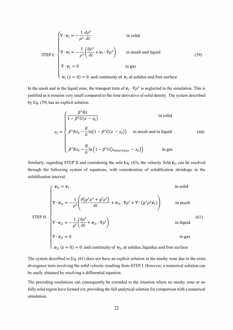
STEP I: { ∇ ∙ 𝒗𝐼 = − 1𝜌𝑠 𝑑𝜌𝑠𝑑𝑡 in solid ∇ ∙ 𝒗𝐼 = − 1𝜌𝑠 (𝜕𝜌𝑠𝜕𝑡 + 𝒗𝐼 ⋅ ∇𝜌𝑠) in mush and liquid ∇ ∙ 𝒗𝐼 = 0 in gas 𝒗𝐼 (𝑧 = 0) = 0 and continuity of 𝒗𝐼 at solidus and free surface

(59)

In the mush and in the liquid zone, the transport term of 𝒗𝐼 ⋅ ∇𝜌𝑠 is neglected in the simulation. This is

justified as it remains very small compared to the time derivative of solid density. The system described

by Eq. (59) has an explicit solution:

𝑣𝐼 ={ 𝛽𝑠𝑅𝑧1 − 𝛽𝑠𝐺(𝑧 − 𝑧𝑆) in solid 𝛽𝑠𝑅𝑧𝑆 − 𝑅𝐺 ln(1 − 𝛽𝑠𝐺(𝑧 − 𝑧𝑆)) in mush and in liquid 𝛽𝑠𝑅𝑧𝑆 − 𝑅𝐺 ln (1 − 𝛽𝑠𝐺(𝑧𝑖𝑛𝑡𝑒𝑟𝑓𝑎𝑐𝑒 − 𝑧𝑆)) in gas

(60)

Similarly, regarding STEP II and considering the sole Eq. (43), the velocity field 𝒗𝐼𝐼 can be resolved

through the following system of equations, with consideration of solidification shrinkage in the

solidification interval:

STEP II:

{ 𝒗𝐼𝐼 = 𝒗𝐼 in solid∇ ∙ 𝒗𝐼𝐼 = − 1𝜌𝑙 (𝜕(𝑔𝑠𝜌𝑠 + 𝑔𝑙𝜌𝑙) 𝜕𝑡 + 𝒗𝐼𝐼 ⋅ ∇𝜌𝑙 + ∇ ∙ (𝑔𝑠𝜌𝑠𝒗𝐼)) in mush∇ ∙ 𝒗𝐼𝐼 = − 1𝜌𝑙 (𝜕𝜌𝑙𝜕𝑡 + 𝒗𝐼𝐼 ⋅ ∇𝜌𝑙) in liquid∇ ∙ 𝒗𝐼𝐼 = 0 in gas𝒗𝐼𝐼 (z = 0) = 0 and continuity of 𝒗𝐼𝐼 at solidus, liquidus and free surface

(61)

The system described in Eq. (61) does not have an explicit solution in the mushy zone due to the extra

divergence term involving the solid velocity resulting from STEP I. However, a numerical solution can

be easily obtained by resolving a differential equation.

The preceding resolutions can consequently be extended to the situation where no mushy zone or no

fully solid region have formed yet, providing the full analytical solution for comparison with a numerical

simulation.

23

3.1.3 Results of numerical simulation and comparison

Fig. 4 shows the reference analytical solution and the simulation results, for both STEP I and STEP II,

at times 0.05 s, 0.3 s, 0.9 s and 1.2 s. Excellent agreement is found. In the mushy zone, after STEP II,

the solidification shrinkage and thermal dilatation of both the solid and liquid phases are accounted for,

while STEP I considers only thermal dilatation of the solid phase. For both STEP I and STEP II, velocity

in the gas domain is constant due to its incompressibility and also equal to the velocity of last liquid

phase.

At time 0.05 s, the solidification has not yet started, the metal is still at fully liquid state (Fig. 4a).

Velocity in the liquid sub-domain is simply due to the thermal dilatation, for both STEP I and STEP II.

In the gas domain, the velocity is constant due to the incompressibility of the gas. Note that, due to the

two-step scheme, only the velocity at the end of STEP II is meaningful.

At time 0.3 s, solidification has started as revealed by the presence of a mushy domain but no fully solid

region has yet formed in the metal domain (Fig. 4b). As expected, there is a uniform gradient of 𝒗𝐼 in

the mush and in the liquid, and a zero gradient in the gas. Regarding 𝒗𝐼𝐼 in the liquid, its gradient is half

the one of 𝒗𝐼 because 𝛽𝑙 is twice lower than 𝛽𝑠. Conversely, in the mush, the gradient of 𝒗𝐼𝐼 is higher

due to solidification shrinkage. This solidification shrinkage consequently explains the large differences

observed in the magnitude of the 𝒗𝐼 and 𝒗𝐼𝐼 velocity fields.

At time 0.9 s and 1.2 s, a full solid region is present in the lower part of the metal sub-domain (Fig. 4c)

while at the latter case (Fig. 4d) the fully liquid metal region disappears and the mushy zone is in contact

with the air domain. The trend is exactly the same as for 0.3 s with, in addition, 𝒗𝐼𝐼 = 𝒗𝐼 in the solid

region, thus verifying application of the Dirichlet boundary condition applied for STEP II. According

to the assumptions, the velocity gradient is thus the same as the one found in the mushy zone for 𝒗𝐼. Small differences exist between the analytical reference solution and the numerical simulation. They are

mainly due to mesh discretization, especially in Fig. 4b and Fig. 4d for STEP II. In fact, mesh is locally

not fine enough to capture the transition between the mushy zone and the liquid sub-domain or gas

domain. In total, the maximum relative error on velocities is 0.55%at time 0.05 s, 2.45%at time 0.3 s, 0.66%at time 0.9 s and 3.96%at time 1.2 s expressing a very good quantitative agreement. The present

test case thus demonstrates the capacity of the partitioned two-step algorithm for predicting velocity

fields in both the solid and the liquid regions.

3.2 Application to ingot filling and cooling

A more practical and relevant application is proposed hereafter, in the context of ingot casting process,

considering realistic material properties. This constitutes a preliminary step to future applications of the

developed model to cases of industrial interest. In particular, it intends to illustrate the added value of

the proposed partitioned solution scheme, considering stages associated to filling and cooling as

encountered in industry. A simple parallelepiped geometry (Fig. 5a) is considered. Liquid steel enters

through the bottom inlet at prescribed temperature 𝑇𝑓𝑖𝑙𝑙 and velocity 𝒗𝑓𝑖𝑙𝑙 . Gas can flow in and out

24

through the upper surface. Heat is extracted from the metal through the sole right-hand lateral surface

using a convection-type expression for heat flux density, 𝑞 = ℎ𝑇(𝑇 − 𝑇𝑒𝑥𝑡), where the heat transfer

coefficient ℎ𝑇 and the external temperature 𝑇𝑒𝑥𝑡 are constant. The metal is supposed to slide along

surrounding surfaces and to stick on the bottom surface except at the liquid inlet surface. The same

mechanical boundary conditions are applied for 𝒗𝐼 and 𝒗𝐼𝐼 for STEP I and STEP II. A symmetry plane

is defined at the left-hand surface and the problem is planar (even if simulations are performed in 3D).

All boundary conditions are summarized in Fig. 5a.

The initial mesh is defined in Fig. 5b, with an adapted isotropic mesh in the bottom metal domain and

coarse mesh in the gas domain. This initial mesh is defined with a simple adaptive meshing computation

based on directional error estimator. This latter makes use of four different fields: the smoothed

Heaviside function, ℋ𝑀, the velocity field from STEP II, 𝒗𝐼𝐼, the temperature field, 𝑇, and the von

Mises equivalent stress from STEP I, �̅�. The chemical composition of the 40CrMnMoS8-6 steel grade

is provided in Table 3. Thermodynamic properties of the material are computed with a thermodynamic

package that makes use of database TCFE6 [31] assuming full equilibrium following the level rule. As

no macrosegregation is considered in the present model, nominal composition is used for any

temperature. For the sake of simplicity, solid behavior over the mushy zone is slightly simplified, with

the mechanical coherency fraction 𝑔𝑐𝑜ℎ𝑙 equal to zero. Properties of material and main parameters are

summarized in Table 4 and in the Appendix.

3.2.1 Ingot filling

Figs. 6(a-c) illustrate the filling stage of the ingot. The zero-isovalue of the level set function

representing the metal/gas interface is shown with the thick green line, as observed in Fig. 6a. As filling

proceeds, the position of the free surface rises until the end of filling at time 2.8 s shown in Fig. 6c. At time 1.0 s, as shown in Fig. 6b, a mushy zone is already formed, with the

liquidus (white line) isotherm near the bottom vertical right-hand surface that defines the metal/mold

boundary. In the mushy zone, the liquid flow penetrates only the uppermost layers below the liquidus

isotherm due to the rapid decrease of permeability with the liquid fraction. In the bulk liquid zone, the

liquid flow moves freely, essentially under the effect of the filling velocity, carrying the cooled down

liquid from the surface to interiors. A small fully solidified layer is already present at time 2.8 s as shown

in Fig. 6c. It is located between the solidus isotherm (the closest white line to the metal/mold boundary)

at the vicinity of the right-hand bottom corner. The stress formed in this thin solid shell can reach about 8 MPa at the end of the filling stage. Fig. 6d shows the adapted mesh at time 2.8 s as a result of the

current magnitude of fields considered in the metric computation. A fine adapted mesh is locally

generated to capture the variation of liquid flow. The mesh is also refined in the solid shell in order to

get more precise information about stress formed in this critical zone. In addition, the mesh is adapted

in an anisotropic way to the smoothed Heaviside function in order to maintain a smooth transition

between gas and metal sub-domains. As the gas sub-domain is not a zone of interest in the present

25

approach, a coarse mesh is imposed to reduce computation time. A discussion on computation time can

be found hereafter in Section 4.1.

3.2.2 Ingot cooling

After filling, the ingot is cooled down under the same heat extraction conditions. The fluid flow and

stresses in the metal domain are shown in Fig. 7 at various later times selected in the same simulation

as Fig. 6. The gas sub-domain is removed for a better view of the metal/gas boundary. It can be seen in

Fig. 7a that liquid flow at 20 s reaching up to 13 mm · s−1 is present mainly in the bulk liquid zone and

in the part of the mushy zone where liquid fraction is high. At the same time, simulation gives access to

stresses in the solidified zone where calculated equivalent stress reaches 120 MPa. However, when the

bulk liquid zone is reduced and the mushy zone is dominant at time 60 s (Fig. 7b), the liquid flow is

considerably slowed down, with values of the order of 2 mm · s−1 . The stress in the solid region

continues to increase near the right-hand surface. As a result of the thermal effect, stress in the solid can

reach about 600 MPa. Note that the velocity field at the metal/gas boundary also reaches about 2 mm ·s−1 at the same time. In fact, properties like density and viscosity are mixed between gas and metal.

Material in the level set transition zone, on the side of gas domain behaves like a fluid. This induces

fluid flow due to the gravity term, especially near the area where borders of mushy zone, solid zone and

gas sub-domain meet and locally the metal/interface forms a descending shape. It may become

problematic when the mushy/gas boundary reaches a critically small value as shown in Fig. 7c at time 96 s. In this situation, the incremental correction distance 𝛿 turns to be excessive because of the very

small correction surface and the updating of the mushy/gas interface with fluid flow derived from STEP

II becomes difficult. Thus, only STEP I is performed after 96 s, the metal/gas boundary being then

updated with velocity from STEP I and incremental mass error being corrected over the whole metal/gas

boundary. Figs. 7(d,e) present respectively the equivalent stress field and temperature field at time 120 s. All metal is now solidified with a highest temperature of 1300 °C, about 130 °C below the

solidus temperature. The maximum of the equivalent stress reaches a value higher than 1000 MPa near

the right-hand cooling surface. Such a high value is commented in the next paragraph. Fig. 7f presents

the final adapted mesh at time 120 s. It shows that the error estimator mesh adaptation method gives

satisfying results. At this final cooling stage, smooth variations of the gradients of the temperature and

velocity fields are computed. Consequently, the mesh is adapted almost exclusively on the stress field

and with the smoothed Heaviside function at the metal/gas boundary.

Stress profiles computed on the domain front surface at height 𝑧 = 20 mm are drawn in Fig. 8 at four

different times. As shown, stress remains very low far from the cooling surface so the representation in

Fig. 8 is limited to a region that extends only 20 mm inward the metal from the cooling surface, e.g. 20 mm < 𝑥 < 40 mm. Fig. 8(a-c) reveal that the stress component in the 𝑥-direction is relatively small

compared to the components in the two other directions. This evolution is explained by the fact that

solidification proceeds in the 𝑥-direction, mainly deriving a �̇�𝑡ℎ contribution that corresponds to the

highest temperature gradient. It contributes little to stress generation. As for stress in the 𝑦-direction at

26

the surface of the simulation domain, tension is observed at all times. One should remind that according

to the planar type boundary conditions, the deformation along the 𝑦-direction cannot be accommodated

and the associated stress component continuously increases with time, reaching almost 700 MPa at 120 s in Fig. 8d. This regular increase of 𝜎𝑦𝑦 is responsible for the high values of �̅� that were noticed

in Fig. 7(c-d). For stress in the 𝑧-direction, the solid shell is firstly loaded in tension at the early stage of

cooling at 10 s. Several millimeters away from the mold surface, compression is found, expressing the

necessary mechanical equilibrium along the vertical direction. This profile is progressively inverted and,

at 120 s, the opposite situation is found with compression of the outer skin and tension of the inner

product. This can be explained by the fact that at the early stage, when solid shell thickness is still small,

the cooling rate of the solid shell is higher at the surface than in depth, due to the release of the latent

heat in the mushy zone. The heat flux extracted from the cooling surface decreases continuously due to

the Fourier-type condition limit. At a later stage, when the solid shell is thick enough, the latent heat

release has little influence on the analyzed 20 mm solid shell near the cooling surface. Therefore the

cooling rate becomes higher in depth than at the cooling surface.

4 Discussions

Beyond the above demonstration of the partitioned two-step solution algorithm, a discussion concerning

simulation time and possible improvement directions is given hereafter.

4.1 Computation time analysis

The computation time is investigated for the academic ingot casting case previously analyzed. The

simulation is performed on 28 Intel® cores with a computation time of 67 h until the process time 96 s with a full two-step algorithm and 12 h from 96 s to 120 s with only STEP I performed. The time

consumption of the different steps of the algorithm is detailed in Table 5 until time 96 s, in order to

analysis the computation efficiency of the full two-step algorithm before complete solidification. Results

show that the remeshing step and level set reset step take considerable resources representing

respectively 27 % and 31 % of the total computation time. The remeshing step is performed at each

time increment in the present simulation. Frequent remeshing is indeed necessary in order to capture the

evolving metal/gas boundary during filling. However the metal/gas boundary is later on relatively stable

as it evolves slowly at each increment during ingot cooling. Frequent remeshing becomes unnecessary.

Management of the remeshing frequency thus becomes an interesting optimization approach to reduce

the computing time.

The level set reset step has also an important cost despite the already optimized direct reinitialization

method. In the present algorithm, a complete reconstruction of the distance function is performed at

each level set reset step. However, only distance over an artificial interface thickness [−𝜀,+𝜀] around

the zero-level set interface is valuable so as to calculate the smoothed Heaviside function. An option

would thus be to reinitiate the distance function only through a certain thickness around the zero-level

set surface, not over the complete domain.

27

Finally, the thermal resolution and the mechanical resolutions STEP I and STEP II represent 39 % of

the total computation time, of which STEP I takes about 58 % of the cost. This is due to the fact that

the resolution of STEP I is non-linear while STEP II is linear. Therefore, another possible option to save

computation time is the desynchronization of STEP I and STEP II, which will be discussed in the

following section.

4.2 Desynchronization of STEP I and STEP II

STEP I and STEP II are performed once in each time increment. However, there is a real interest in

desynchronizing the two resolutions. Indeed, in many casting applications, the solid-oriented resolutions

could be performed less often than the liquid-oriented ones, because of different characteristic time

scales. Moreover, influence of STEP I to STEP II is much smaller than that of STEP II to STEP I. The

direct momentum transfer from solid movement to fluid flow remains small compared to the influence

of STEP II to STEP I via the heat and mass transfer by fluid flow. For instance, with a STEP I performed

only once for each two time increments, computation time can be reduced by at least 10 % and even

more if optimization is expected by combination of the remeshing and level set steps.

4.3 Mass conservation of the metal domain

In the present partitioned algorithm, mass conservation problem is observed. Fig. 9 shows the time

evolution of the deviation of the total mass from its value over the first 96 s of the simulation. Without

mass correction, the total metal mass globally decreases until about time 50 s and then continuously

increases until 96 s. The relative mass error reaches a maximum value of about 1.3 %. While limited,

this mass loss must be corrected. Its origin essentially lies in the use of the level set method in the context

of a solidification process. The velocity field used to transport the metal/gas interface is not exact, it is

an approximation obtained by considering a transition zone around this interface, with mixed material

properties. As a consequence, the capture of the motion of the metal/gas interface by the level set method

may result in non-conservation of metal mass. Certainly there exist other issues like finite element

discretization, time discretization, and mesh adaptation, which drive also the non-conservation of the

total metal mass. Therefore, it was proposed to implement an incremental mass correction method in

the present algorithm, as described in Section 2.4.

The mass correction method was tested in the previous ingot casting simulation. When mass correction

method is applied, the total metal mass is well conserved. One should consider that, with the present

methodology, the correction of the level set position at each time increment remains of the order of few 𝜇m. This is 1000 times lower than the artificial level set thickness used in the simulation. Hence,

application of this correction method in the partitioned resolution algorithm has almost no influence on

the calculated fluid flow and solid stress, while keeping a good metal mass conservation.

4.4 Compressive behavior of the mushy zone

In the STEP I solution, the selected constitutive model for metal in the mushy state consists of an

extrapolation of the constitutive model of the fully solid metal at higher temperatures. Currently, this is

28

achieved by simply extending the temperature dependence of the constitutive parameters, such as 𝐾 and 𝑚. Possible alternatives could be made available in future developments to better capture the movement

of the columnar dendritic structure in the mush. An interesting approach would consist in introducing a

dependence of these constitutive parameters with respect to the solid fraction, together with

compressible viscoplasticity by use of a compressible viscoplastic potential. This was actually done by

Bellet and coworkers in a 2D finite element model with a concurrent resolution (in a single non-linear

set of equations) of liquid velocity, solid velocity and liquid pressure for the study of liquid/metal

interactions in the mushy zones [32,33]. In this approach the constitutive model for the solid phase was

inspired from the work of Suéry and coworkers [34,35]. A similar approach has been developed by

Ludwig et al. [36] in a 2D finite volume discretization, with, in addition, the modelling of the transport

and sedimentation of equiaxed grains in the melt. Beckermann and coworkers [37,38], also used a

compressible viscoplastic constitutive model, but restricted their resolution to the solid phase

deformation in the mushy zone, without interaction with the melt. Interest of such an extension would

also lie in the possibility to make use of the intrinsic properties of each solid phase formed upon

solidification. Indeed, all possible solid phases forming are made accessible thanks to tabulation of the

solidification path by using a thermodynamic database. With potentially different intrinsic mechanical

properties of different solid phases, averaging of the behavior of the phases would also be possible, that

would then no longer depend on the total fraction of solid alone. Coupling with microsegregation models

would also then be made accessible, which was shown to be crucial for the prediction of

macrosegregation [39].

5 Conclusions

In this paper an original solution scheme has been proposed in view of solving concurrently solid

mechanics and fluid flow in the context of the numerical modelling of solidification processes. This is

a very challenging objective, because of huge differences in the order of magnitude of stress, velocities

and mechanical stiffness characterizing bulk liquid regions on one hand and fully solidified regions on

the other hand. Up to the knowledge of the authors, this problem had not been satisfactorily solved so

far.

The model presented in this paper consists of a partitioned solution scheme. At each time increment a

solid-oriented solution is performed first, followed by a liquid-oriented one. Both solution schemes are

formulated in the finite element method, with a level set tracking of the moving interface between the

solidifying metal and the surrounding gas. The successive resolutions are tightly coupled and operated

on a common spatial discretization of the whole analysis domain: metal and gas. The first resolution –

solid-oriented – is in charge of providing the velocity field, and the associated strains and stresses arising

from the highly non-linear elastic-viscoplastic deformation of the solidified regions. The second

resolution – liquid oriented – is in charge of providing the velocity field arising from the liquid flow,

governed by Navier-Stokes equations with Darcy damping in the mushy zones. A detailed presentation

of the sets of equations, and of their weak forms with level set formulation has been given.

29

The two-step solver was first validated in the context of directional solidification: the proposed

algorithm provided solutions in excellent agreement with reference solutions. Then it was applied to the

context of ingot casting. It was demonstrated that the proposed scheme was able to solve the entire

process: first the filling stage, during which stress and strains can be captured in the fine solid skin

formed, together with the forced fluid flow; second the cooling stage after filling, with stress and strains

in bulk solid regions, together with thermally convected flow in bulk liquid regions and mushy zone.

The accurate capture of these phenomena was achieved thanks to continuous remeshing all along the

process simulation, the local density of the mesh being determined by a multi-objective metric tensor.

The limitations of the present approach essentially lie in the treatment of contact with molds. At present,

there is a strong hypothesis of non-departure of the solidified skin from the mold surface. In a short term

future, this should be taken into account by implementing a penalty treatment of the non-penetration

condition.

The main perspectives of this work are twofold. First, besides the ingot casting application, the proposed

solution will be extended to the continuous casting process. This will require the implementation of an

Arbitrary Lagrangian-Eulerian (ALE) scheme, using mobile meshes in the interval between two

successive remeshing steps. Second, the coupling of the proposed two-step solver with the solution of

chemical species conservation, gas flow and grain motion will give access to enhanced predictions of

macrosegregation due to thermosolutal convection, shrinkage flow, transport of equiaxed grains [40]

and thermomechanical deformation of solid and mushy regions. Together with the demonstrated

efficient coupling of thermohydraulic and thermomechanical effects on heat and total mass transport,

this is expected to provide engineers with radically new simulation methods and packages for

optimization of industrial casting processes.

Acknowledgements

This work was funded by the European Space Agency – ESTEC (Netherlands) under the projects

CCEMLCC (Grant AO-2004-017) and industrial partners ARCELORMITTAL Maizières Research,

APERAM ALLOYS IMPHY and INDUSTEEL.

30

References

[1] M. Heil, A. L. Hazel, J. Boyle, Solvers for large-displacement fluid-structure interaction

problems: segregated versus monolithic approaches, Comput. Mech. 43 (2008) 91-101 [2] M. Bellet, V. D. Fachinotti, ALE method for solidification modelling, Computer Methods in

Applied Mechanics and Engineering 193, 39-41 (2004) 4355-4381 [3] M. Bellet, O. Jaouen, I. Poitrault, An ALE-FEM approach to the thermomechanics of

solidification processes with application to the prediction of pipe shrinkage, International Journal of Numerical Methods for Heat and Fluid Flow 15, 2-3 (2005) 120-142

[4] A. Saad, Ch.-A. Gandin, M. Bellet, Temperature-based energy solver coupled with tabulated thermodynamic properties - Application to the prediction of macrosegregation in multicomponent alloys, Computational Materials Science 99 (2015) 221-231

[5] S. Osher, J.A. Sethian, Fronts Propagating with Curvature Dependent Speed: Algorithms Based on Hamilton-Jacobi Formulations, Journal of Computational Physics 79 (1988) 12-49

[6] J. A. Sethian, P. Smereka, Level-Set methods for fluid interfaces, Annual Review of Fluid Mechanics, 35 (2003) 341-372

[7] A. Saad, Ch.-A. Gandin, M. Bellet, T. Volkmann, D. Herlach, Simulation of shrinkage-induced macrosegregation in a multicomponent alloy during reduced-gravity solidification, TMS2016 Annual Meeting Supplemental Proceedings (2016) 35-42

[8] M. Shakoor, B. Scholtes, P.-O. Bouchard, M. Bernacki, An efficient and parallel level set reinitialization method – Application to micromechanics and microstructural evolutions, Applied Mathematical Modelling 39 (2015) 7291-7302

[9] J. A. Dantzig, M. Rappaz, Solidification, EPFL Press, Lausanne (2009) [10] P. Vicente-Hernandez, Vers une approche thermomécanique du procédé de fonderie:

caractérisation rhéologique et microstructurale d'alliages métalliques à l'état semi-solide (Towards a thermomechanical approach of casting processes: rheological and microstructural charcterization of metallic alloys in the semi-solid state), Ph.D. Thesis (in French), École Nationale Supérieure des Mines de Paris, 1994

[11] M. Bellet, B.G. Thomas, Solidification macroprocesses (Thermal - Mechanical modeling of stress, distorsion and hot tearing), in Materials Processing Handbook, J.R. Groza, J.F. Shackelford, E.J. Lavernia and M.T. Powers (eds.), Chapter 27, CRC Press, Taylor and Francis (2007) 27-1 – 27-26

[12] B. G. Thomas, M. Bellet, Modeling of stress, distortions and hot tearing, in ASM Handbook Volume 15: Casting, American Society of Metals (2008) Division 4: Modeling and Analysis of Casting Processes, 449-461

[13] D. N. Arnold, F. Brezzi, M. Fortin, A stable finite element for Stokes equation, Calcolo 21 (1984) 337-352

[14] P. I. Babuška, Error-bounds for finite element method, Numerische Mathematik 16, 4 (1971) 322-333

[15] F. Brezzi, On the existence, uniqueness and approximation of saddle-point problems arising from Lagrangian multipliers, ESAIM: Mathematical Modelling and Numerical Analysis-Modélisation Mathématique et Analyse Numérique 8, R2 (1974) 129-151

[16] M. Bellet, Optimisation du changement de variable sur la pression pour les formulations éléments finis vitesse-pression de Thercast® et R2sol, Technical note (in French), Mines ParisTech – CEMEF (2003), 4 pages, internal communication

[17] S. Ganesan, D. R. Poirier, Conservation of Mass and Momentum for the Flow of Interdendritic Liquid during Solidification, Metallurgical Transactions B 21 (1990) 173-181

[18] J. Ni, C. Beckermann, A Volume-Averaged Two-Phase Model for Transport phenomena during Solidification, Metallurgical Transactions B 22 (1991) 349-361

[19] M. Rappaz, M. Bellet, M. Deville, Numerical modeling in materials science and engineering, Springer-Verlag, Berlin Heidelberg (2003)

[20] S. Gouttebroze, Modélisation 3D par éléments finis de la macroségrégation lors de la solidification d'alliages binaires (3D finite element modeling of macrosegregation upon

31

solidification of binary alloys), Ph.D. Thesis (in French), Ecole Nationale Supérieure des Mines de Paris (2005)

[21] S. Gouttebroze, M. Bellet, H. Combeau, 3D macrosegregation simulation with anisotropic remeshing, C. R. Mecanique 335, 5-6 (2007) 269-279

[22] W. G. Gray, K. O’Neill, On the general equations for flow in porous media and their reduction to Darcy’s law, Water Resources Research 12(1976) 148-154

[23] S. Whitaker, Flow in Porous Media I: A theoretical derivation of Darcy’s law, Transport in Porous Media 1 (1986) 3-25

[24] P. C. Carman, Fluid flow through granular beds, Chemical Engineering Research and Design: Transactions of the Institution of Chemical Engineers Part A, 37 (1937) 2069-2079.

[25] M. Bellet, Modélisation thermomécanique des procédés de déformation plastique et de solidification, (Thermomechanical modeling of processes involving plastic deformation and solidification), Mémoire d'Habilitation à Diriger des Recherches (in French), Université de Nice – Sophia Antipolis (2005)

[26] T. E. Tezduyar, S. Mittal, S. E. Ray, R. Shih, Incompressible flow computations with stabilized bilinear and linear equal-order-interpolation velocity-pressure elements, Computer Methods in Applied Mechanics and Engineering 95 (1992) 221-242

[27] T. E. Tezduyar, Y. Osawa, Finite element stabilization parameters computed from element matrices and vectors, Computer Methods in Applied Mechanics and engineering 190 (2000) 411-433

[28] E. Hachem, Stabilized Finite Element Method for Heat Transfer and Turbulent Flows inside Industrial Furnaces, Ph.D. Thesis, Mines ParisTech (2009)

[29] E. Hachem, B. Rivaux, T. Kloczko, H. Digonnet, T. Coupez, Stabilized finite element method for incompressible flows with high Reynolds number, J. Comp. Phys. 229 (2010) 8643-8665

[30] T. Coupez, Metric construction by length distribution tensor and edge based error for anisotropic adaptive meshing, Journal of Computational Physics . 230 (2011) 2391-2405

[31] TCFE6: A thermodynamic database for different kinds of steels and Fe-based alloys.Thermo-Calc Software AB, 2010, Stockholm, SE

[32] V. D. Fachinotti, S. Le Corre, N. Triolet, M. Bobadilla, M. Bellet, Two-phase thermo-mechanical and macrosegregation modelling of binary alloys solidification with emphasis on the secondary cooling stage of steel slab continuous casting, Int. J. Num. Meth. Eng. 67 (2006) 1341-1384

[33] T. Koshikawa, M. Bellet, Ch.-A. Gandin, H. Yamamura, M. Bobadilla, Study of hot tearing during steel solidification through ingot punching test and its numerical simulation, Metallurgical and Materials Transactions A 47 (2016) 4053-4067

[34] T. G. Nguyen, D. Favier, M. Suéry, Theoretical and experimental study of the isothermal mechanical behavior of alloys in the semi-solid state, Int. J. Plasticity 10 (1994) 663–693

[35] C. L. Martin, D. Favier, M. Suéry, Viscoplastic behaviour of porous metallic materials saturated with liquid, Part I: constitutive equations, Int. J. Plasticity 13 (1997) 215 –235

[36] A. Ludwig, A. Vakhrushev, T. Holzmann, M. Wu, A. Karicha, Two-phase modelling of equiaxed crystal sedimentation and thermomechanic stress development in the sedimented packed bed, Proc. MCWASP XIV, 14th Int. Conf. on Modeling of Casting, Welding and Advanced Solidification Processes, Awaji Island, Japan, 21-26 June 2015, H. Yasuda (ed.), IOP Conference Series: Materials Science and Engineering 84 (2015) 012102

[37] C. A. Monroe, C. Beckermann, J. Klinkhammer, Modeling of Casting, Welding, and Advanced Solidification Processes-XII, Edited by: Steve L. Cockcroft and Daan M. Maijer,TMS (2009) 313-320

[38] M. G. Pokorny, C.A. Monroe, C. Beckermann, Z. Zhen, N. Hort, Simulation of Stresses during Casting of Binary Magnesium-Aluminum Alloys, Metallurgical and Materials Transactions A 41 (2010) 3196-3207

[39] T. Koshikawa, M. Bellet, Ch.-A. Gandin, H. Yamamura, M. Bobadilla, Experimental study and two-phase numerical modelling of macrosegregation induced by solid deformation during punch pressing of solidifying steel ingots, Acta Materialia 124 (2017) 513-527

[40] T.-T.-M. Nguyen, Ch.-A. Gandin, H. Combeau, M. Založnik, M. Bellet, Finite element multi-scale modelling of chemical segregation in steel solidification taking into account the transport of equiaxed grains, Metallurgical and material transactions A 49 (2018) 1725-1748

32

Appendix

The following figures detail the physical and materials properties of the 40CrMnMoS8-6 steel grade

used in the present computations.

33

Illustrations captions

Fig. 1. Schematic of a representative volume element in the context of solidification with (a) distribution

of regions of metal and the surrounding gas, (b) the smoothed Heaviside function based on the level set

method used for tracking the metal/gas boundary, (c) the parameters of the constitutive model for the

metal sub-domain, (d) the Heaviside function based on a temperature parameter to distinguish the

regions of metal with TEVP and TVP mechanical behaviors.

Fig. 2. Resolution scheme on a time increment.

Fig. 3. Test case for model validation with (a) geometric configuration and boundary conditions and (b)

initial mesh.

Fig. 4. Vertical profiles of the vertical components of computed velocities 𝒗𝐼 and 𝒗𝐼𝐼 for the test case at

time (a) 0.05 s, (b) 0.3 s, (c) 0.9 s and (d) 1.2 s with (plain lines) the analytical reference solution and

(lines with symbols) the numerical simulation.

Fig. 5. Geometry of ingot case simulation with (a) initial configuration of the ingot during the filling

stage and boundary conditions and (b) initial mesh. Note the non-symmetric boundary conditions along

the left and right vertical walls.

Fig. 6. Snapshot of solidification simulation showing on the front surface (a-c) a time sequence of the

evolution of the temperature field, 𝑇, and fluid velocity, 𝑣𝐼𝐼, in the metal sub-domain during the filling

stage. Evolutions are presented at times (a) 0.1 s, (b) 1 s and (c) 2.8 s and corresponding (d) adapted

mesh and (e) equivalent stress field, �̅�, in a small region close to the cooling wall at time 2.8 s. The

liquidus and solidus temperature isotherms are highlighted with thick white lines in (a-c) and (e), while

the iso-level set value 𝜑 = 0 that represents the metal/gas boundary is highlighted in green in (a-c). Note

that the left vertical wall is a symmetry plane.

Fig. 7. Time evolution of the equivalent stress field, �̅� in the metal sub-domain during the cooling stage

at times (a) 20 s, (b) 60 s , (c) 96 s and (d) 120 s; corresponding (e) temperature field and (f) adapted

mesh at time 120 s. Fluid velocity, 𝑣𝐼𝐼, is also shown on (a) and (b) when liquid domain is still present

in ingot. The liquidus and solidus temperature isotherms are highlighted with thick white lines. The

fields in the gas sub-domain are not shown.

Fig. 8. Stress components along the three directions x, y, z are plotted at different process times (a) 10 s,

(b) 20 s, (c) 60 s, and (d) 120 s, along a horizontal profile at height z = 20 mm and y = 2.5 mm. Stress

curves are shown only for the right part of the profile between x = 20 mm (ingot center) and x = 40 mm

(right lateral wall), as they are null along the left part of the profile (liquid state).

Fig. 9. Time evolution of the relative error on metal mass conservation without and with correction.

34

Fig. A.1: Evolution of the liquid fraction 𝑔𝑙 in the solidification interval

Fig. A.2: Evolution of the solid density 𝜌𝑠 (until liquidus temperature) and the liquid density 𝜌𝑙 (until

solidus temperature) as a function of temperature.

Fig. A.3: Evolution of the specific solid enthalpy ℎ𝑠 and specific liquid enthalpy ℎ𝑙 as a function of

temperature

Fig. A.4: Evolution of the solid consistency 𝐾 as a function of temperature

Fig. A.5: Evolution of the solid strain rate sensibility 𝑚 as a function of temperature

Fig. A.6: Evolution of the solid hardening coefficient 𝑛 as a function of temperature

Fig. A.7: Evolution of the Young modulus 𝐸 as a function of temperature

Fig. A.8: Evolution of the yield stress 𝝈𝒀 as a function of temperature

Tables captions:

Table 1: Expressions of the different mixed properties according to the region considered.

Table 2: Values of material and numerical parameters used in unidirectional solidification test case.

Table 3: Composition of the steel grade.

Table 4: Material, simulation and numerical parameters used in ingot casting. All tabulations are

provided as graphs in the Appendix.

Table 5: Distribution of the computation time for the ingot casting simulation at process time 96 s.

1

(a) (b)

(c) (d)

Fig. 1. Schematic of a representative volume element in the context of solidification with (a) distribution of

regions of metal and the surrounding gas, (b) the smoothed Heaviside function based on the level set method

used for tracking the metal/gas boundary, (c) the parameters of the constitutive model for the metal

sub-domain, (d) the Heaviside function based on a temperature parameter to distinguish the regions of metal

with TEVP and TVP mechanical behaviors (see main text).

1

Fig. 2. Illustration of an element at interface �� with �� representing the cutting interface by zero-isovalue of

the level set function �.

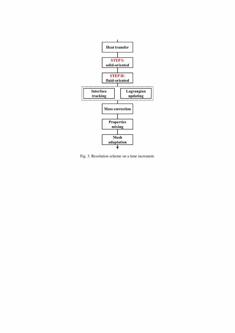
Fig. 3. Resolution scheme on a time increment.

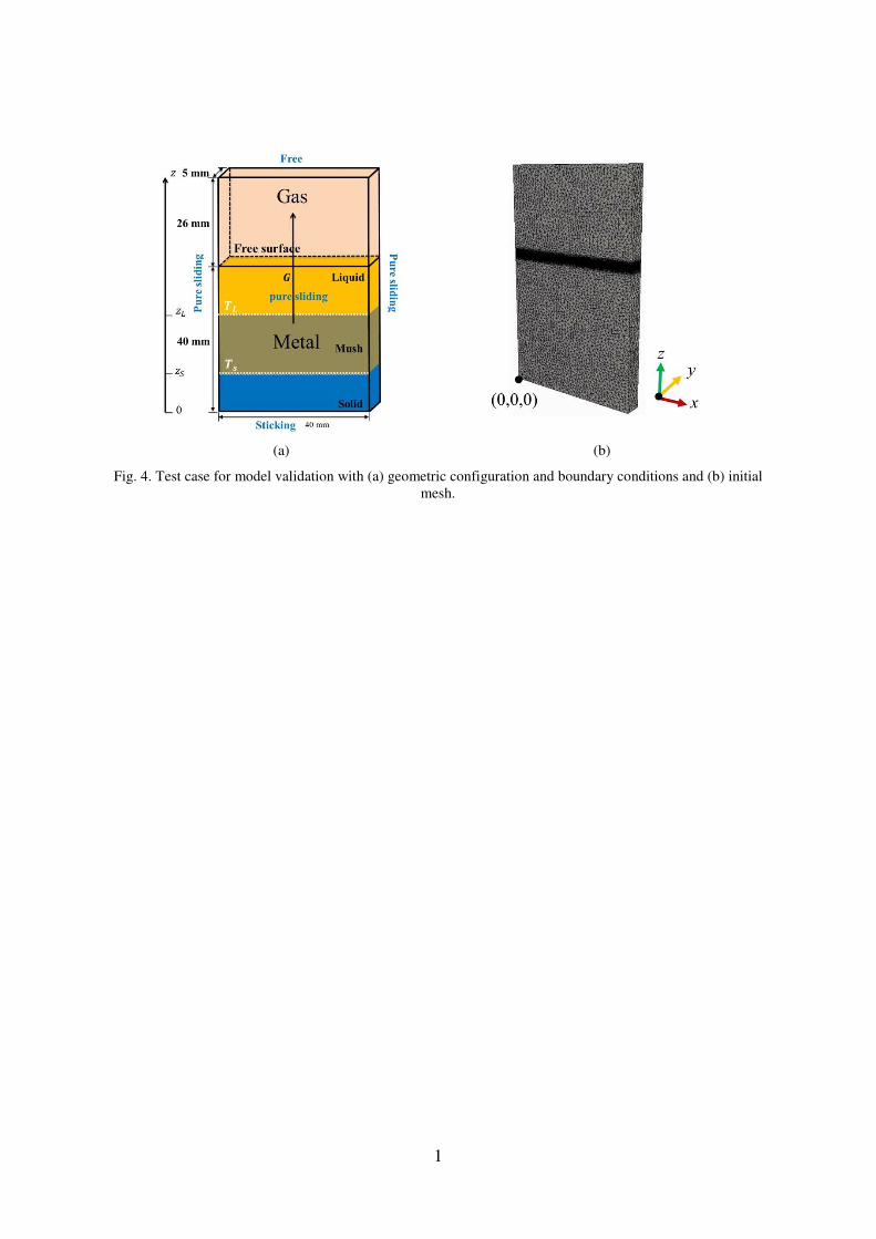
1

(a) (b)

Fig. 4. Test case for model validation with (a) geometric configuration and boundary conditions and (b) initial

mesh.

1

(a) (b)

(c) (d)

Fig. 5. Vertical profiles of the vertical components of computed velocities �� and ��� for the test case at time (a)

0.05 s , (b) 0.3 s , (c) 0.9 s and (d) 1.2 s with (plain lines) the analytical reference solution and (lines with

symbols) the numerical simulation.

1

(a) (b)

Fig. 6. Geometry of ingot case simulation with (a) initial configuration of the ingot during the filling stage and

boundary conditions and (b) initial mesh.

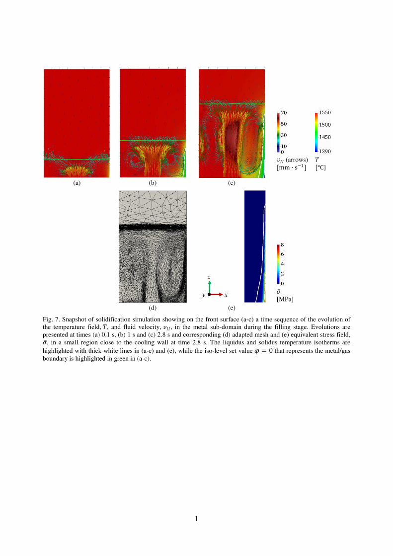
1

��� (arrows)

[mm · s�]

�

[°C]

(a) (b) (c)

��

[MPa]

(d) (e)

Fig. 7. Snapshot of solidification simulation showing on the front surface (a-c) a time sequence of the evolution of

the temperature field, �, and fluid velocity, ���, in the metal sub-domain during the filling stage. Evolutions are

presented at times (a) 0.1 s, (b) 1 s and (c) 2.8 s and corresponding (d) adapted mesh and (e) equivalent stress field,

��, in a small region close to the cooling wall at time 2.8 s. The liquidus and solidus temperature isotherms are

highlighted with thick white lines in (a-c) and (e), while the iso-level set value � = 0 that represents the metal/gas

boundary is highlighted in green in (a-c).

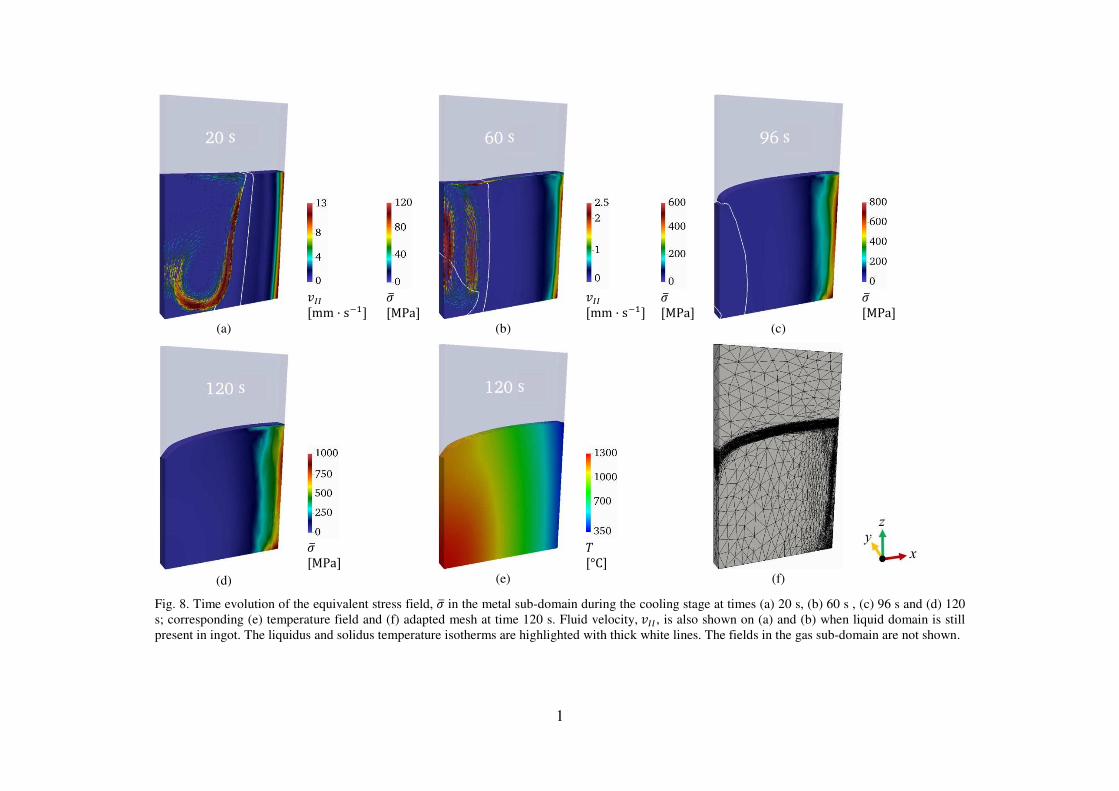
1

���

�mm � s�

��

�MPa

���

�mm � s�

��

�MPa

��

�MPa

(a) (b) (c)

��

�MPa

�

�°C

(d) (e) (f)

Fig. 8. Time evolution of the equivalent stress field, �� in the metal sub-domain during the cooling stage at times (a) 20 s, (b) 60 s , (c) 96 s and (d) 120

s; corresponding (e) temperature field and (f) adapted mesh at time 120 s. Fluid velocity, ��� , is also shown on (a) and (b) when liquid domain is still

present in ingot. The liquidus and solidus temperature isotherms are highlighted with thick white lines. The fields in the gas sub-domain are not shown.

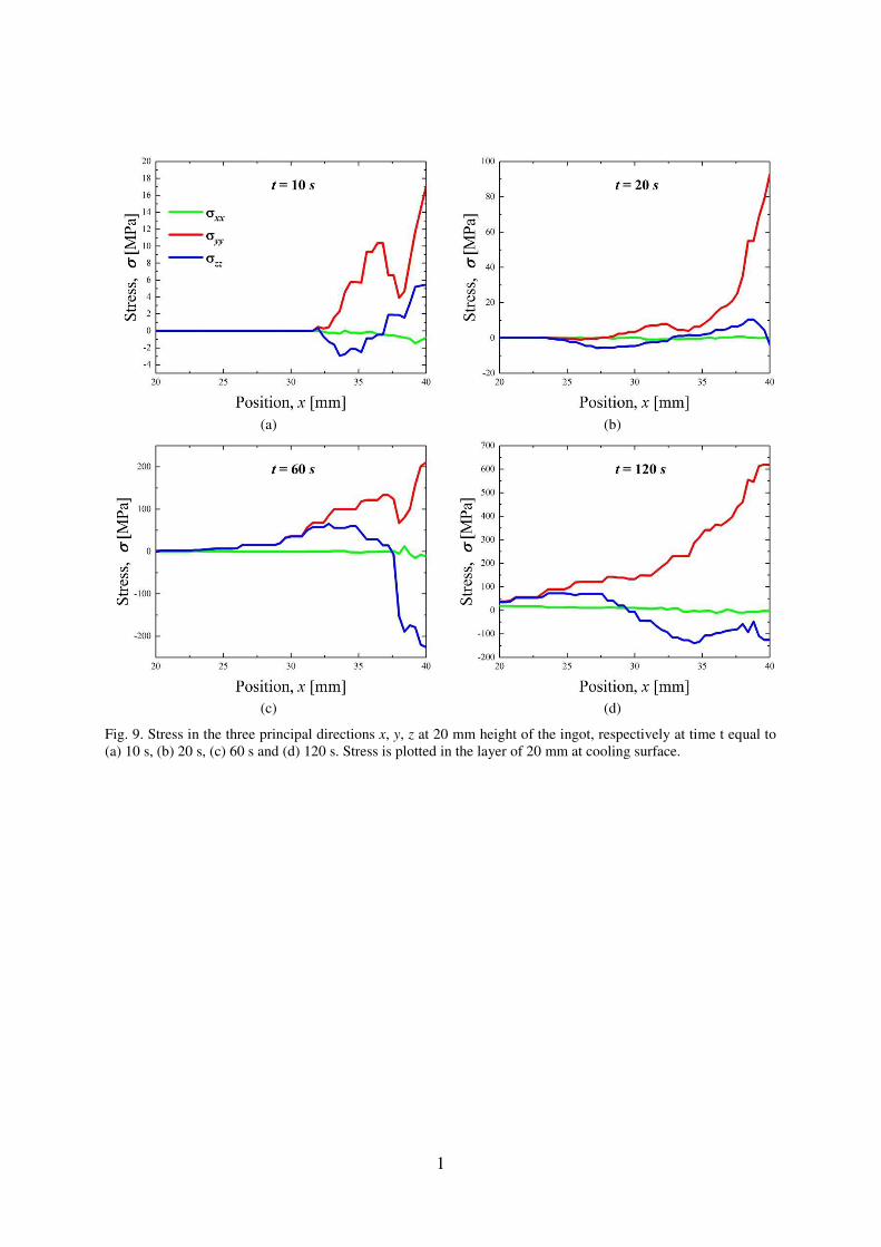
1

(a) (b)

(c) (d)

Fig. 9. Stress in the three principal directions x, y, z at 20 mm height of the ingot, respectively at time t equal to

(a) 10 s, (b) 20 s, (c) 60 s and (d) 120 s. Stress is plotted in the layer of 20 mm at cooling surface.

1

Fig. 10. Time evolution of the relative error on metal mass conservation without

and with correction.

1

Fig. A.1: Evolution of the liquid fraction �� in the solidification interval

1

Fig. A.2: Evolution of the solid density 𝜌𝑠 (until liquidus temperature) and the liquid density 𝜌𝑙 (until solidus

temperature) as a function of temperature.

1

Fig. A.3: Evolution of the specific solid enthalpy ℎ𝑠 and specific liquid enthalpy ℎ𝑙 as a function of temperature

1

Fig. A.4: Evolution of the solid consistency 𝐾 as a function of temperature

1

Fig. A.5: Evolution of the solid strain rate sensibility 𝑚 as a function of temperature

1

Fig. A.6: Evolution of the solid hardening coefficient 𝑛 as a function of temperature

1

Fig. A.7: Evolution of the Young modulus 𝐸 as a function of temperature

1

Fig. A.8: Evolution of the yield stress 𝜎𝑌 as a function of temperature

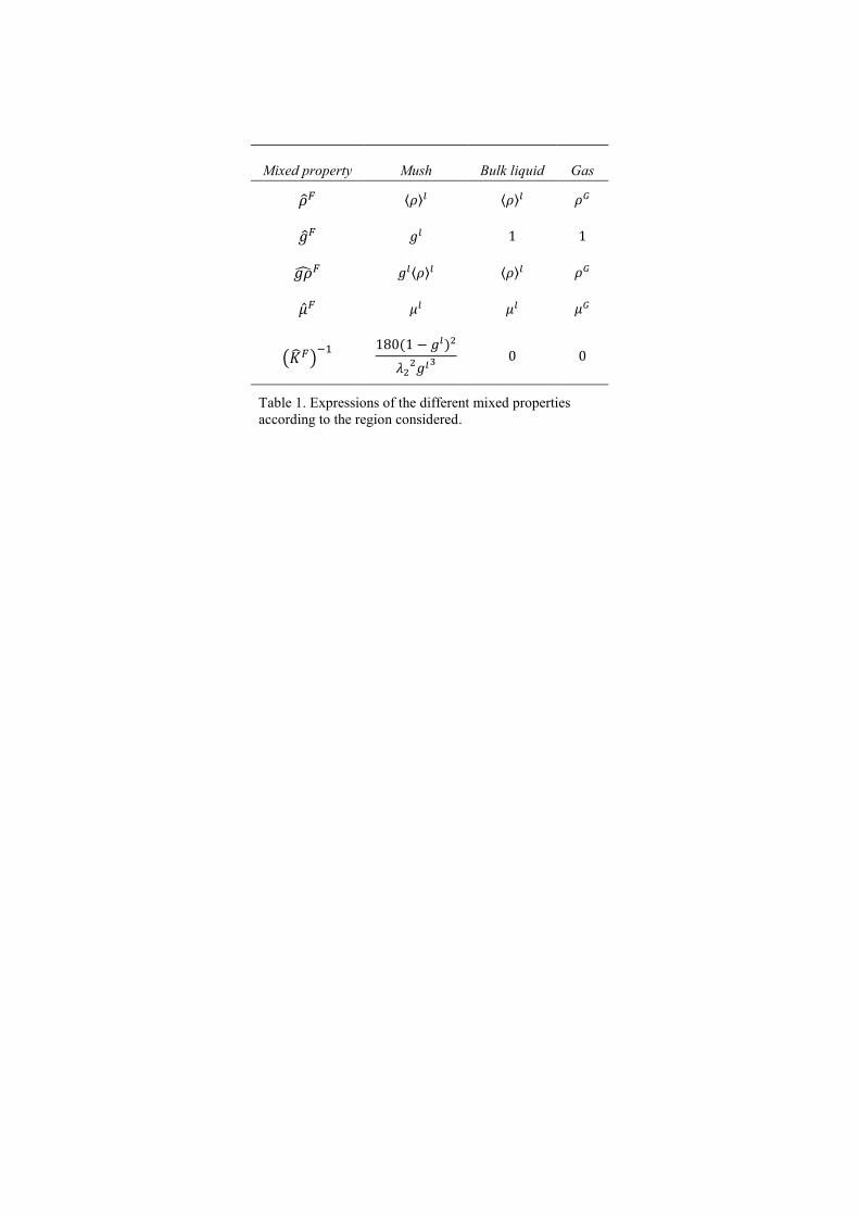
Mixed property Mush Bulk liquid Gas �̂�𝐹 ⟨𝜌⟩𝑙 ⟨𝜌⟩𝑙 𝜌𝐺 𝑔𝐹 𝑔𝑙 1 1 𝑔�̂�𝐹 𝑔𝑙⟨𝜌⟩𝑙 ⟨𝜌⟩𝑙 𝜌𝐺 �̂�𝐹 𝜇𝑙 𝜇𝑙 𝜇𝐺

(�̂�𝐹)−1 180(1 − 𝑔𝑙)2𝜆22𝑔𝑙3 0 0

Table 1. Expressions of the different mixed properties

according to the region considered.

1

Material parameter Symbol Value Unit

Initial bottom temperature 𝑇0𝑏𝑜𝑡 1773.15 K

Vertical temperature gradient 𝐺 3030.30 K · m−1

Cooling rate 𝑅 −100 K · s−1

Solidus temperature 𝑇𝑆 1704.15 K

Liquidus temperature 𝑇𝐿 1763.65 K

Solid density at solidus 𝜌𝑆 8000 kg · m−3

Liquid density at liquidus 𝜌𝐿 6000 kg · m−3

Gas density 𝜌𝐺 6000 kg · m−3

Solid dilatation coefficient 𝛽𝑠 4 × 10−4 K−1

Liquid dilatation coefficient 𝛽𝑙 2 × 10−4 K−1

Gas viscosity STEP I | STEP II 𝜇𝐺 100 | 100 Pa · s

Liquid viscosity STEP I | STEP II 𝜇𝑙 100 | 100 Pa · s Solid consistency 𝐾 100 Pa · s

Numerical parameter

Level set thickness 𝜀 1 mm

Time step ∆𝑡 0.01 s Table 2. Values of material and numerical parameters used in unidirectional

solidification test case.

Element C Mn Cr Mo Si Fe

wt.% 0.4 1.5 2 0.2 0.3 Balance

Table 3. Composition of the steel grade.

Material parameter Symbol Value Unit

Solidus temperature 𝑇𝑆 1704.15 (1431) K (°C)

Liquidus temperature 𝑇𝐿 1763.65 (1490.5) K (°C)

Reference temperature 𝑇𝑟𝑒𝑓 1763.65 (1490.5) K (°C)

Liquid density at liquidus 𝜌𝐿 7001.82 kg · m−3

Solid density 𝜌𝑠 𝑇𝑎𝑏𝑢𝑙𝑎𝑡𝑖𝑜𝑛 kg · m−3

Gas density 𝜌𝐺 1.3 kg · m−3

Liquid dilatation coefficient 𝛽𝑙 9.23 × 10−5 K−1

Secondary dendritic arm spacing 𝜆2 5 × 10−4 m

Gas viscosity STEP I | STEP II 𝜇𝐺 100 | 1 × 10−5 Pa · s

Liquid viscosity STEP I | STEP II 𝜇𝑙 100 | 5 × 10−3 Pa · s

Solid consistency 𝐾 𝑇𝑎𝑏𝑢𝑙𝑎𝑡𝑖𝑜𝑛 Pa · sm

Poisson’s ratio 𝜈 0.3 −

Strain rate sensibility 𝑚 𝑇𝑎𝑏𝑢𝑙𝑎𝑡𝑖𝑜𝑛 −

Hardening coefficient 𝑛 𝑇𝑎𝑏𝑢𝑙𝑎𝑡𝑖𝑜𝑛 −

Young modulus 𝐸 𝑇𝑎𝑏𝑢𝑙𝑎𝑡𝑖𝑜𝑛 MPa

Yield stress 𝜎𝑌 𝑇𝑎𝑏𝑢𝑙𝑎𝑡𝑖𝑜𝑛 MPa

Simulation parameter

Initial temperature 𝑇𝑖𝑛𝑖𝑡 1823.15 (1550) K (°C)

Filling temperature 𝑇𝑓𝑖𝑙𝑙 1823.15 (1550) K (°C)

External temperature 𝑇𝑒𝑥𝑡 293.15 (20) K (°C)

Filling velocity 𝑣𝑓𝑖𝑙𝑙 5 × 10−2 m · s−1

Heat transfer coefficient ℎ𝑇 3000 W · m−2 · K−1

Numerical parameter

Level set thickness 𝜀 1 mm

Time step ∆𝑡 0.01 s

Table 4. Material, simulation and numerical parameters used in ingot casting. All

tabulations are provided as graphs in the Appendix.

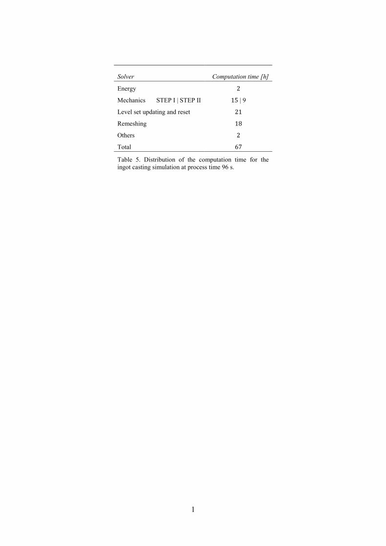
1

Solver Computation time [h]

Energy 2

Mechanics STEP I | STEP II 15 | 9

Level set updating and reset 21

Remeshing 18

Others 2

Total 67

Table 5. Distribution of the computation time for the

ingot casting simulation at process time 96 s.