a parallel simulated annealing algorithm zbigniew j. …cdn.intechweb.org/pdfs/10764.pdf · a...

A parallel simulated annealing algorithm as a tool for itness landscapes exploration 247

A parallel simulated annealing algorithm 4pt as a tool for itness landscapes exploration

Zbigniew J. Czech

0

A parallel simulated annealing algorithm

as a tool for fitness landscapes exploration

Zbigniew J. CzechSilesia University of Technology and University of Silesia

Poland

1. Introduction

Solving a discrete optimization problem consists in finding a solution which maximizes (orminimizes) an objective function. The function is often called the fitness and the correspond-ing landscape the fitness landscape. We are concerned with statistical measures of a fitnesslandscape in the context of the vehicle routing problem with time windows (VRPTW). Themeasures are determined by using a parallel simulated annealing algorithm as a tool for ex-ploring a solution space. This chapter summarizes our experience in designing parallel simu-lated annealing algorithms and investigating fitness landscapes of a sample NP-hard bicrite-rion optimization problem.Since 2002 we have developed several versions of the parallel simulated annealing (SA) al-gorithm (11)-(19). Each of these versions comprises a number of parallel SA processes whichco-operate periodically by passing and exploiting the best solutions found during the search.For this purpose a specific scheme of co-operation of processes has been devised. The meth-ods of parallelization of simulated annealing are discussed in Aarts and van Laarhoven (2),Aarts and Korst (1), Greening (20), Abramson (3), Boissin and Lutton (8), and Verhoeven andAarts (35). Parallel simulated annealing to solve the VRPTW is applied by Arbelaitz et al. (4).Onbasoglu and Ozdamar (26) present the applications of parallel simulated annealing algo-rithms in various global optimization problems. The comprehensive study of parallelizationof simulated annealing is given by Azencott et al. (5)The parallel SA algorithm allowed us to discover the landscape properties of the VRPTWbenchmarking tests (33). This knowledge not only increased our understanding of processeswhich happen during optimization, but also helped to improve the performance of the parallelalgorithm. The usage of the landscape notion is traced back to the paper by Wright (37). Themore formal treatments of the landscape properties are given by Stadler (32), Hordijk andStadler (22), Reidys and Stadler (31). Statistical measures of a landscape are proposed byWeinberger (36). The reviews of the landscape issues are given by Reeves (30) and Reeves andRowe (29).Section 2 of this chapter formulates the optimization problem which is solved. Section 3 de-scribes a sequential SA algorithm. In section 4 two versions of the parallel SA algorithm, calledindependent and co-operating searches, are presented. Section 5 is devoted to the statisticalmeasures of the fitness landscapes in the context of the VRPTW. In subsections 5.1-5.2 somebasic notions are introduced, and in subsection 5.3 the results of the experimental study arediscussed. Section 6 concludes the chapter.

13

www.intechopen.com

Parallel and Distributed Computing248

2. Problem formulation

The VRPTW is an extension to the capacitated vehicle routing problem (CVRP) which is for-mulated as follows (34). There is a central depot of goods and n customers (nodes) geograph-ically scattered around the depot. The locations of the depot (i = 0) and the customers (i = 1,2, . . . , n), as well as the shortest distances dij and the corresponding travel times tij betweenany two customers i and j are given. Each customer asks for a quantity qi of goods which hasto be delivered (or picked up from) by a vehicle of capacity Q. Because of this capacity limit,the vehicle after serving a subset of customers has to return to the depot for reloading. Thevehicle effects the whole service on a number of routes. Each route starts and terminates at thedepot. A solution to the CVRP is a set of routes of minimum travel distance (or travel time)which visits each customer i, i = 1, 2, . . . , n, exactly once. The total demand for each routecannot exceed Q.The CVRP is extended into the VRPTW by introducing for each customer and the depot aservice time window [ei, fi] and a service time si (s0 = 0). The values ei and fi determine, re-spectively, the earliest and the latest time for start servicing. The customer i has to be servedwithin the time window [ei, fi] and the service of all customers should be accomplished withinthe time window of the depot [e0, f0]. The vehicle can arrive to the customer before the timewindow but then it has to wait until time ei, when the service can begin. The latest time for ar-rival of the vehicle to customer i is fi. It is assumed that the routes are traveled simultaneouslyby a fleet of K homogeneous vehicles (i.e. of equal capacity), each vehicle assigned to a singleroute. A solution to the VRPTW is the set of routes which guarantees the delivery of goodsto all customers and satisfies the time window and vehicle capacity constraints. Furthermore,the size of the set equal to the number of vehicles needed (primary objective) and the totaltravel distance (secondary objective) should be minimized.More formally, there are three types of decision variables in this two-objective optimizationproblem. The first decision variable, xi,j,k, i, j ∈ {0,1, . . . ,n}, k ∈ {1,2, . . . ,K}, i �= j, is 1 if vehiclek travels from customer i to j, and 0 otherwise. The second decision variable, ti, denotes thetime when a vehicle arrives at customer i, and the third decision variable, bi, denotes thewaiting time at that customer. The aim is to:

minimize K, and then (1)

minimize ∑ni=0 ∑

nj=0,j �=i ∑

Kk=1 di,jxi,j,k, (2)

subject to the following constraints:

K

∑k=1

n

∑j=1

xi,j,k = K, for i = 0, (3)

n

∑j=1

xi,j,k =n

∑j=1

xj,i,k = 1, for i = 0 and k ∈ {1,2, . . . ,K}, (4)

K

∑k=1

n

∑j=0,j �=i

xi,j,k =K

∑k=1

n

∑i=0,i �=j

xi,j,k = 1, for i, j ∈ {1,2, . . . ,n}, (5)

www.intechopen.com


n

∑i=1

qi

n

∑j=0,j �=i

xi,j,k ≤ Q, for k ∈ {1,2. . . . ,K} (6)

K

∑k=1

n

∑i=0,i �=j

xi,j,k(ti + bi + hi + ti,j) ≤ tj, for j ∈ {1,2, . . . ,n} (7)

and t0 = b0 = h0 = 0,

ei ≤ (ti + bi) ≤ fi, for i ∈ {1,2, . . . ,n}. (8)

Formulas (1) and (2) define the minimized functions. Eq. (3) specifies that there are K routesbeginning at the depot. Eq. (4) expresses that every route starts and ends at the depot. Eq. (5)assures that every customer is visited only once by a single vehicle. Eq. (6) defines the capacityconstraints. Eqs. (7)–(8) concern the time windows. Altogether, eqs. (3)–(8) define the feasiblesolutions to the VRPTW.Lenstra and Rinnooy Kan (24) proved that the VRP and the VRPTW are NP-hard discreteoptimization problems.

3. Sequential simulated annealing

The algorithm of simulated annealing which can be regarded as a variant of local search wasfirst introduced by Metropolis et al. (25), and then used to optimization problems by Kirk-patrick, Gellat and Vecchi (23), and Cerny (10). A comprehensive introduction to the subjectcan be found in Reeves (27) and Azencott (5).Let C : S �→ R be a cost function which is to be minimized, defined on some finite solutionset (search space) S. Let N(X), N(X) ⊂ S, be a set of neighbors of solution X for each X ∈ S.Usually the sets N(X) are small subsets of S. For the VRPTW the members of N(X) areconstructed by moving one or more customers among the routes of solution X. The wayin which these sets are created influences substantially the accuracy of results obtained by asimulated annealing algorithm. While constructing the sets N(X) we make sure that theirmembers are built through deep modifications of X. Let R be a transition probability matrix,such that R(X,Y) > 0 if and only if Y ∈ N(X). Let (Ti), i = 0, 1, . . . be a sequence of positivenumbers, called the temperatures of annealing, such that Ti ≥ Ti+1 and limi→∞ Ti = 0. Thesequence (Ti) is called the cooling schedule, and a sequence of annealing steps within whichthe temperature of annealing stays constant is called the cooling stage. Consider the sequentialannealing algorithm for constructing a sequence (or chain) of solutions (Xi), Xi ∈ S, definedas follows. An initial solution X0 is computed using e.g. some heuristics. Given the currentsolution Xi, a potential next solution Yi is chosen from set N(Xi) with probability R(Xi,Yi).Then in a single annealing step solution Xi+1 is set as follows (cf. Fig. 2):

Xi+1 =

Yi if C(Yi) ≤ C(Xi),Yi with probability pi, if C(Yi) > C(Xi),Xi otherwise,

wherepi = exp(−(C(Yi)− C(Xi))/Ti). (9)

www.intechopen.com


If Xi+1 is set to Yi and C(Yi) > C(Xi), then we say that an uphill move is carried out. Eq. (9)implies that uphill moves are performed more often when temperature Ti is high. When Ti isclose to zero uphill moves occur sporadically. Simulated annealing can be described formallyby non-homogeneous Markov chains. In these chains the probability of moving from one stateto another depends not only on these states but also on the temperature of annealing.A solution X ∈ S is said to be a local minimum of the cost function C, if C(X)≤ C(Y) for all Y ∈N(X), and to be a global minimum of C, if C(X) = infY∈S C(Y). Let Smin be the set of globalminima of C. We say that the process of simulated annealing converges, if limi→∞

P(Xi ∈Smin) = 1. It was proved (21) that the convergence is guaranteed by the logarithmic coolingschedules of the form: Ti ≥

Rlog(i+1)

for some constant R which depends on the cost function

landscape. It was also shown (5; 9) that for the logarithmic cooling schedules the speed ofconvergence is given by:

P(Xi /∈ Smin) ∼

(

K

i

)α

(10)

for i large enough, where K > 0 and α > 0 are suitable constants. Both constants are connectedto the cost function landscape, and for large solution spaces constant K is very large and con-stant α is very small (5; 9). This implies that the process of simulated annealing converges veryslowly. According to Eq. (10) a global minimum is attained only if the process of annealing isinfinite. For this reason the question of how to accelerate simulated annealing by making useof parallelism is crucial.In the sequential simulated annealing algorithm to solve the VRPTW, the chain (Xi) is con-structed in two phases. The goal of phase 1 is to minimize the number of routes of the VRPTWsolution, whereas phase 2 minimizes the total length of the routes. However in phases 1 and 2it may happen that both the number of routes and the total length of routes are reduced. Thecost of solution Xi in phase 1 is computed as: C1(Xi) = c1N + c2D + c3(r1 − r), and in phase 2as: C2(Xi) = c1N + c2D, where N is the number of routes (vehicles) of solution Xi, D – the totaltravel distance of the routes, r1 – the number of customers of a randomly chosen route whichis to be shorten and perhaps eliminated from the current solution, r – the average numberof customers in all routes, c1, c2, c3 – some constants. For simplicity, instead of the logarith-mic an exponential cooling schedule is used, i.e. the temperature of annealing is decreased asTk+1 = β f Tk, for k = 0, 1, . . . , a f , and some constants β f (β f < 1) and a f ( f = 1 and 2 denotephase 1 and 2).

4. Parallel simulated annealing algorithm

4.1 Independent searches

In the parallel algorithm of independent searches (IS), p independent simulated annealingprocesses P0, P1, . . . , Pp−1 are executed. Every process performs its computations like inthe sequential algorithm. On completion, the processes pass their best solutions found to themaster process, which selects the best solution among solutions it received. This solutionconstitutes the final result of the IS algorithm.More formally, suppose that i steps of sequential simulated annealing is taken. Then in parallelIS, p annealing chains of z = i/p steps each are executed. As the result p terminal solutions{Xz,0, Xz,1, . . . , Xz,p−1} are computed, from which the final solution Yi is selected by: Yi =Xz,0 ⊗ Xz,1 ⊗ . . . ⊗ Xz,p−1, where ⊗ is the operator of choosing the better solution with respect

www.intechopen.com


to the total length of routes1. In terms of convergence we have (5):

P(Yi /∈ Smin) = ∏0≤j≤p−1

P(Xz,j /∈ Smin). (11)

Assuming that each simulated annealing chain j of z steps converges at speed determined by

Eq. 10: P(Xz,j /∈ Smin) ∼(

Kz

)α, we get (5):

P(Yi /∈ Smin) ∼

(

Kp

i

)αp

. (12)

Consider a chain of i = 107 steps of sequential simulated annealing, and let K = 100 and α =

0.01. Then according to Eq. 10 the speed of convergence is equal(

Ki

)α≈ 0.89. If one uses p =

5, 10, 15 and 20 processes, then by Eq. (12) the speeds of convergence of IS are:(

Kpi

)αp≈ 0.61,

0.40, 0.27 and 0.18, respectively. Thus the parallel independent searches converge much fasterthan the sequential algorithm.

4.2 Co-operating searches

The parallel algorithm of co-operating searches (CS) executes in the form of p processes P0,P1, . . . , Pp−1 (Figs. 1-3). A process generates its own annealing chain divided into two phases(lines 6–19 in Fig. 1). A phase consists of a number of cooling stages, and a cooling stageconsists of a number of annealing steps. The processes co-operate with each other every ωannealing step passing their best solutions found to date (lines 12–16 in Fig. 1, and Fig. 3). Thechain of annealing steps of process P0 is entirely independent (Fig. 4). The chain of processP1 is updated at steps uω, u = 1, 2, . . . , um, to the better solution between the best solutionsfound by processes P0 and P1 to date. Similarly, process P2 chooses as the next point in itschain the better solution between its own best and the one obtained from process P1. Thusthe best solution found by process Pl is piped down for further enhancement to processesPl+1 . . . Pp−1. Clearly, after step umω process Pp−1 holds the best solution Xb found by allthe processes. To our best knowledge the speed of convergence of co-operating searches givene.g. by equations similar to Eq. (10) and (12) are not known.As mentioned before, the temperature of annealing decreases according to the equationTk+1 = β f Tk for k = 0, 1, 2, . . . , a f , where a f is the number of cooling stages. In this work weinvestigate two cases in establishing the points of process co-operation with respect to tem-perature drops. In the first case, of regular co-operation, processes interact at the end of eachcooling stage (ω = L) (lines 12–13 in Fig. 1). The number of annealing steps executed withina cooling stage is set to L = (5E)/p, where E = 105 is a constant established experimentally,and p = 5, 10, 15 and 20, is the number of processes (line 3 in Fig. 1). Such an arrangementkeeps the parallel cost of the algorithms constant when different numbers of processes areused, provided the co-operation costs are neglected. Therefore in this case as the number ofprocesses becomes larger, the length of cooling stages goes down, what means that the fre-quency of co-operation increases. In the second case, of rare co-operation, the frequency isconstant and the processes exchange their solutions every ω = E annealing step (lines 14–15in Fig. 1). For the number of processes p = 10, 15 and 20, the co-operation takes place after 2,3 and 4 temperature drops, respectively.

1 In this analysis it is assumed that each chain achieves a solution with the minimum (best known) num-ber of routes.

www.intechopen.com


1 parfor Pj, j = 0, 1, . . . , p − 1 do

2 Set co-operation mode to regular or rare depending on a test set;3 L := (5E)/p; {establish the length of a cooling stage; E = 105}4 Create the initial solution using some heuristics;5 current solutionj := initial solution; best solutionj := initial solution;

6 for f := 1 to 2 do {execute phase 1 and 2}{beginning of phase f}

7 T := T0, f ; {initial temperature of annealing}

8 repeat {a cooling stage}9 for i := 1 to L do10 annealing step f (current solutionj, best solutionj);

11 end for;12 if ( f = 1) or (co-operation mode is regular) then {ω = L}13 co operation;14 else {rare co-operation: ω = E}15 Call co operation procedure every E annealing step

counting from the beginning of the phase;16 end if;17 T := β f T; {temperature reduction}

18 until a f cooling stages are executed;

{end of phase f}19 end for;20 end parfor;21 Produce best solutionp−1 as the solution to the VRPTW;

Fig. 1. Parallel simulated annealing algorithm of co-operating searches

1 procedure annealing step f (current solution, best solution);

2 Create new solution as a neighbor to current solution(the way this step is executed depends on f );

3 δ := C f (new solution)−C f (current solution);

4 Generate random x uniformly in the range (0, 1);5 if (δ < 0) or (x < e−δ/T) then6 current solution := new solution;7 if C f (new solution) < C f (best solution) then

8 best solution := new solution;9 end if;10 end if;11 end annealing step f ;

Fig. 2. Annealing step procedure

The exchange of solutions between processes can be considered as exploitation of the searchresults, whereas exploration takes place when a process penetrates the search space freely. Letus call a sequence of ω annealing steps executed by a process between points of co-operationas a chain of free exploration. Taking into account Eq. (10) the longer these chains the better.

www.intechopen.com


1 procedure co operation;2 if j = 0 then Send best solution0 to process P1;3 else {j > 0}4 receive best solutionj−1 from process Pj−1;

5 if C f (best solutionj−1) < C f (best solutionj) then

6 best solutionj := best solutionj−1;

7 current solutionj := best solutionj−1;

8 end if;9 if j < p − 1 then Send best solutionj to process Pj+1; end if;

10 end if;11 end co operation;

Fig. 3. Procedure of co-operation of processes

X0 →

X(0)0 → X

(ω)0 → X

(2ω)0 → • • → X

(umω)0

↓ ↓ ↓

X(0)1 → X

(ω)1 → X

(2ω)1 → • • → X

(umω)1

↓ ↓ ↓

• • • • • •

• • • • • •

X(0)p−2 → X

(ω)p−2 → X

(2ω)p−2 → • • → X

(umω)p−2

↓ ↓ ↓

X(0)p−1 → X

(ω)p−1 → X

(2ω)p−1 → • • → X

(umω)p−1 → Xb

Fig. 4. Scheme of co-operation of processes (X0 – initial solution; Xb – best solution among theprocesses)

Note that due to co-operation, a process after having completed a chain with solution X, maybe forced to explore the search space from a—probably more promising—solution differentfrom X. In order to obtain good results during parallel search the proper balance betweenexploitation and exploration has to be maintained.A series of experiments was carried out in order to establish how the number of processes,the length of chains of free exploration, and the frequency of processes co-operation influencethe accuracy of solutions to the VRPTW (16). For the experiments, 39 out of 56 benchmarkingtests2 elaborated by Solomon (33) were used. The tests are grouped into three major problemsets named R, C and RC. The geographical coordinates for customers in sets R, C and RC aregenerated randomly, in a clustered manner, and as a mix of random and clustered structures,respectively. Each of these sets is divided into two subsets, R1, R2, C1, C2, RC1, RC2. Thesubsets R1, C1 and RC1 have short time windows and permit relatively large numbers ofroutes (between 9 and 19) in the solutions. The time windows for subsets R2, C2 and RC2are wider allowing less routes (between 2 and 4) in the solutions. Every test involves 100customers and the distances are measured using Euclidean metric. It is assumed that traveltimes are equal to the corresponding distances.

2 The tests in set C are easy to solve, so they were omitted in the experiments.

www.intechopen.com


In the series of the experiments, the IS and CS algorithms3 were executed at least 1000 timesfor each test, a given number of processes p, a number of annealing steps L2 fixed for it,and a period of communication ω. Based on each sample of results4 the average of totaltravel distances of routes y and the standard deviation s were calculated. The experimentsshowed that depending on the test instance, the minimum of the mean value y appeared fordifferent values of parameters p, L2 and ω. E.g. the minimum of y for test R101 was obtainedfor p = 20 and L2 = ω = E/4 (Table ??). Whether these specific values of parameters give

p L2 ω R101 R102 R103 R104 R105 R106

5 E E 13.9 17.6 11.4 0.8 1.1 10.6

10 E/2 E/2 6.5 11.6 3.9 0.5 0.1 5.3

15 E/3 E/3 1.4 3.3 min 0.7 2.3 2.120 E/4 E/4 min∗ min∗ 0.6∗ min 0.3 min

10 E/2 E 10.3 13.6 5.5 0.7 1.4 6.7

15 E/3 E 15.3 19.9 9.7 1.1 1.0 3.0

20 E/4 E 13.8 20.1 8.8 0.6∗ min∗ 0.9∗

p L2 ω R107 R108 R109 R110 R111 R112

5 E E 0.8 1.0 min∗ min∗ 0.3 1.2

10 E/2 E/2 min 0.1 6.5 3.2 min 1.1

15 E/3 E/3 1.1 min 6.7 3.7 1.4 min

20 E/4 E/4 0.7∗ 1.2∗ 10.4 5.3 1.9∗ 0.8

10 E/2 E 1.9 1.5 4.1 2.7 1.5 1.6

15 E/3 E 3.1 2.7 8.8 3.6 3.0 0.7

20 E/4 E 4.6 4.2 10.3 5.5 3.6 1.3∗

Table 1. Values of test statistic Z for CS algorithm and set R1;’*’ marks the best choice ofparameters p, L2 and ω

statistically superior results can be proved by testing the hypotheses H0 : µi ≤ µm versus analternative hypothesis Ha : µi > µm, where µ denotes the mean value of a population of totaltravel distances of routes; i – populations whose samples have worse mean values (e.g. casesp = 5 and L2 = ω = E; p = 10 and L2 = ω = E/2; etc. for test R101); m – a population forwhich the minimum mean value of a sample was observed (i.e. case p = 20 and L2 = ω = E/4for test R101). In the cases where H0 are rejected one can claim that their values of parametersp, L2 and ω give inferior solutions with respect to the values for which y = ymin occur, orequivalently, the population with y = ymin comprises superior solutions as compared to other

3 It was observed (15) that for some Solomon’s tests the probability of finding a solution with the min-imum number of routes was very low. Therefore phase 1 of the algorithms was executed in the CSfashion with a1 = 50 cooling stages and L1 = 105 annealing steps in each stage. In phase 2 the IS and CSmodes were used with a2 = 100 and L2 depending on the number of processes. The following valuesof parameters were fixed: c1 = 40000, c2 = 1, c3 = 50, β1 = 0.95, β2 = 0.98.

4 For some tests the size of the sample was smaller than 1000, since only solutions with the minimumnumber of routes were considered.

www.intechopen.com


A. p L2 ω R109 R110 R202 RC102 RC104 RC108 RC202

5 E – 2.1∗ 2.7 5.6 2.4 3.0 min∗ 3.3

IS 10 E/2 – 2.9 4.8 9.4 4.0 6.5 8.5 4.4

15 E/3 – 6.8 6.5 12.0 5.2 11.1 13.6 3.6

20 E/4 – 8.8 9.5 13.1 6.3 11.7 20.3 4.5

5 E E min min∗ min∗ min min∗ 2.4 min∗

CS 10 E/2 E/2 6.5 3.2 7.2 0.8∗ 2.7 7.1 4.0

15 E/3 E/3 6.7 3.7 10.4 3.4 5.2 12.1 6.7

20 E/4 E/4 10.4 5.3 12.8 4.1 8.2 15.2 8.2

10 E/2 E 4.1 2.7 4.7 5.3 3.3 5.1 2.5

CS 15 E/3 E 8.8 3.6 7.8 3.5 6.2 10.4 3.4

20 E/4 E 10.3 5.5 9.7 4.3 6.8 13.6 3.9

Table 2. Values of test statistic Z for IS and CS algorithms

populations. For the test statistic:

Z =yi − ym

√

s2i

ni+ s2

mnm

the hypotheses H0 are rejected at the α = 0.01 significance level, if Z > Z0.01 = 2.33 (ni andnm are numbers of experiments over which si and sm values are calculated). Table ?? showsthe values of Z for set R1 (results for sets R2, RC1 and RC2 are reported in (16)), where minindicates values of p, L2 and ω which give the minimum of y. The framed values denoterejections of hypotheses H0, what means that for the corresponding values of parameters p,L2 and ω, the results of statistically worse total travel distances of routes are achieved. It canbe seen that the values of Z for test R101 and parameters p = 15, L2 = ω = E/3, and p = 20,L2 = ω = E/4, are less than 2.33. So it is justified to claim that these values of parameters givestatistically the best solutions to the VRPTW. In other words, using p = 20 or 15 processes co-operating after every cooling stage enable us to obtain quickly solutions of the best accuracy.It follows from the experiments (16) that for most Solomon’s tests the results of high accuracycan be achieved by making use of p = 20 processes. The exceptions are tests R109, R110, R202,RC102, RC104, RC108 and RC202. For these tests the minimum of y occurs when p = 5 andmost of other numbers of processes yield statistically worse results. As already indicated,to keep the cost of parallel computations constant, the number of annealing steps taken byprocesses between points of co-operation was decreased along with an increase of the numberof processes. The results of the experiments prove that for the tests listed above the executionof shorter annealing chains of free exploration of length from L2 = E/4 to L2 = E/2 are notcompensated—in terms of accuracy—by the co-operation between processes.The annealing chains of free exploration are substantially longer in the algorithm of inde-pendent searches (IS), in which the processes do not co-operate and execute chains as longas L2 = Ea2, where a2 is the fixed number of cooling stages5. Table 2 compares the resultsobtained by the IS and CS algorithms for the specific tests mentioned above. It can be seenthat an increase of the length of chains and lack of co-operation in the IS algorithm, make

5 Note that altogether each process of the IS and CS algorithms executes a1 + a2 cooling stages.

www.intechopen.com


the results worse for tests R110, R202, RC104 and RC202. Applying the IS algorithm—of lowcommunication cost—can be justified only for tests R109 and RC108.Considering the results of the experiments and the objective of computing good quality solu-tions to the VRPTW in a short time, Solomon’s tests can be divided into 3 groups:

I – tests which can be solved quickly (e.g. using p = 20 processes) to good accuracy withrare co-operation (ω = E). To this group belong 24 tests, out of 39, not listed in groupsII and III specified below.

II – tests which can be solved quickly (e.g. with p = 20) but the co-operation should takeplace after every cooling stage (we call this co-operation regular) (e.g. ω = E/4 for p =20) to achieve good accuracy of solutions. This group comprises 8 tests: R101, R102,R103, R107, R108, R111, R207 and RC105.

III – tests whose solving cannot be accelerated as much as for the tests in groups I andII. The solutions of best accuracy are obtained for less than p = 20 processes6. To thisgroup belong 7 tests: R109, R110, R202, RC102, RC104, RC108 and RC202.

5. Fitness landscape

5.1 Basic definitions

Let C, S and N(X) be a cost function, a search space and a set of neighbors of solution X,respectively, as defined in section 3. A solution Xo ∈ S is said to be a local minimum offunction C, if C(Xo) ≤ C(Y) for all Y ∈ N(Xo), and to be a global minimum X∗ of C, ifC(X∗) = infY∈S C(Y). In evolutionary optimization function C is often called the fitness andthe associated landscape a fitness landscape. More formally (29), a landscape L for the func-tion C is a triple L = (S,C,d) where d denotes a distance measure d : S × S �→ R

+ ∪ {∞}which for any solutions P, Q, R ∈ S satisfies the conditions: d(P, Q) ≥ 0, d(P, Q) = 0 ⇔ P = Qand d(P, R)≤ d(P, Q)+ d(Q, R). If d is symmetric, i.e. d(P, Q)= d(Q, P) for all P, Q ∈ S then dis a metric on space S.Discrete optimization can be performed by neighborhood search where the process of search-ing starts at some initial solution and converges to a local optimum, or an attractor. Thesearching process is described by a function µ : S �→ So, where X ∈ S is an initial solutionand µ(X) is the optimum that it reaches (29). A basin of attraction of solution Xo is the setB(Xo)= {X : µ(X)= Xo}. The set contains the initial solutions from which the search leads toa specified attractor. The basins of attraction for a given function are not unique. They dependon a method adopted for landscape exploration and can be established only if the method isdeterministic. Therefore the notion of the basin is of limited use for methods with a good dealof randomization, like simulated annealing.

5.2 Statistical measures of fitness landscape

The nature of a fitness landscape can be unveiled either by mathematical analysis or by gath-ering some statistical data during the process of searching it. In this work we follow the latterapproach. Several statistical measures have been proposed in the literature. Weinberger (36)observed that some characteristics could be obtained from a random walk. Let Ct be the fit-ness of the solution visited at time t. Then the autocorrelation function of the landscape during

6 There are two open questions here: whether less than p = 5 processes could give solutions of betteraccuracy for some tests in group III, and whether finding solutions for tests in groups I-II can be speededup even further by making use of more than p = 20 processes with no loss of solutions accuracy.

www.intechopen.com


a random walk of length T is:

aj =∑

T−jt=1 (Ct − C)(Ct+j − C)

∑Tt=1(Ct − C)2

where C is the mean fitness of the T solutions visited, and j is the lag. For smooth landscapes,with neighbor solutions of similar fitness, and small lags, the values of aj are close to 1. As thelag increases the values of autocorrelation are likely to diminish. The values of aj are close tozero at all lags for rugged landscapes, where close solutions have unrelated fitness.A useful indicator of the difficulty of an optimization problem is the number of optima ap-pearing in a corresponding landscape. Indeed, the more optima in the landscape, the harderis to find the global optimum. Suppose that for a given optimization problem the search isrestarted r times with random initial solutions. Most likely these solutions lay in differentbasins of attraction, so as the result of the search a number of different local solutions k, k ≤ r,will be found. Based on the values of r and k one may estimate the number of optima ν presentin a given landscape. Assuming that the probability of encountering each solution is the same,it is easy to show that the random variable K which takes the number of distinct solutions ina series of r independent searches has the Arfwedson distribution (28):

P[K = k] =ν!

(ν − k)! νrrk (13)

where 1 ≤ k ≤ min(r,ν), with the mean:

EK = ν[1 − (1 − 1/ν)r]. (14)

After having measured EK one can solve numerically Eq. (14) and find an estimate for ν.Reeves (28) gives an approximation of it as: ν ≈ (K2 − r)/(2(r − K)), where K is a measuredestimation of EK. When the value of ν is small one may ask how many searches W should bedone to be sure with some certainty that all optima have been found. The waiting time Wk

for the (k + 1)th solution provided that k of them have been already found has a geometricdistribution, and the mean of the waiting time for ν solutions is (28):

EW ≈ ν(lnν + γ) (15)

where γ ≈ 0.577 is Euler’s constant. The formulas (13)–(15) are derived under the assumptionthat the probability of encountering each solution is the same, or in other words that solutionsare isotropically distributed in the landscape. Unfortunately in many optimization problems,also in the VRPTW, this assumption is not valid.

5.3 Experimental study

The objective of the study was to gather statistical data concerning the fitness landscapes for39 (out of 56) VRPTW tests by Solomon.

Fitness landscape characteristics

In the course of experiments the parallel simulated annealing algorithm was executed at least4200 times (see column Exp. in Table 4) for each test in sets R and RC. The VRPTW is a two-objective optimization problem in which both, the number of routes and the total travel dis-tance, should be minimized. For the landscape studies only solutions with the minimum

www.intechopen.com


number of routes were taken into account. Most of Solomon’s tests are relatively easy to solvewith respect to the first objective function (the exceptions are tests R104, R112, RC101, RC105,and RC106, see paragraph “Difficulty of test instances”). The minimum number of routes foreach test is generally known. Since the VRPTW problem is NP-hard, there is some probabilitythat these numbers are not global minima. However for simplicity, we shall name them as‘minima’ instead of ‘known minima’.Table 3 contains the histograms of numbers of solutions7 produced by the algorithm withthe total travel distance y worse by 0-1%, 1-2% etc. than the distance ymin of the best-knownsolution. The columns denoted by τ and τmax show the values of (y − ymin)/ymin and (ymax −

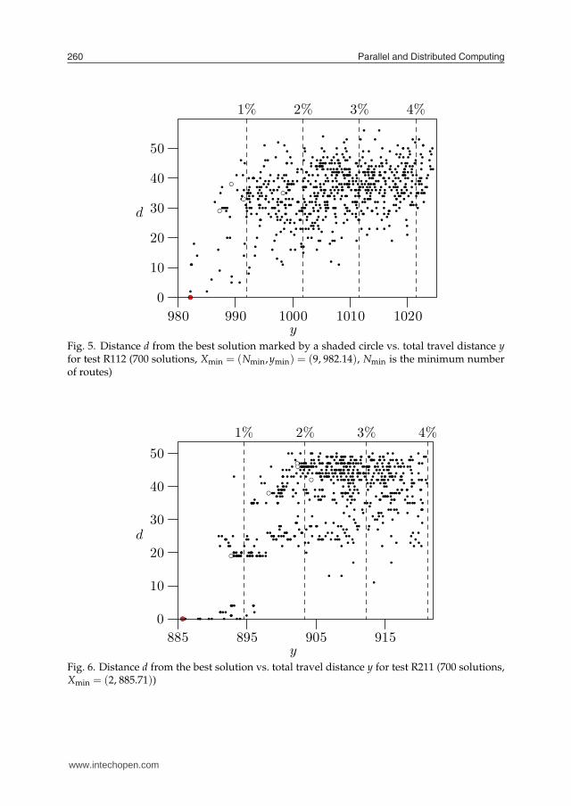
ymin)/ymin, where y and ymax are the average and maximum total travel distances obtainedfor a given test, respectively. All values in Table 3 are expressed in per cents, and the tests areordered according to 0-1% column. It can be seen e.g. for test R112 that there is 30% chanceof getting a solution with distance y worse by 2-3% than ymin. This is because the number ofdistinct solutions in terms of y for this test, discovered in ranges from 0-1% to >4% were 102,149, 179, 89 and 81, respectively. Clearly, the distribution of solutions in the fitness landscapeis not isotropic, i.e. they are not uniformly scattered across every direction in the search space.There exists a relatively large number of solutions with y ∈ [1.02ymin,1.03ymin), what increasesthe probability that the algorithm will finish its computations at a local optimum with y inthis range. Fig. 5 plots the distances d of a sample of solutions from the best solution foundXmin, against the total travel distances of solution routes8. As a metric for measuring thedistance d between solutions we use the minimum number of customer movements amongthe routes necessary to convert one solution into another (see subsection 5.1). It was observedthat the solutions of all VRPTW tests were not sampled with equal probability. For instance,the majority of solutions of test R1129 were hit only a few times, but 5 solutions were reachedat least 10 times (marked by white circles in Fig. 5). Most likely the sizes of basins of attractionof more popular solutions are larger, although the notion of such a basin is vague in the contextof simulated annealing where random uphill moves may take place. The characteristics of thefitness landscape depend also on the search algorithm. Note that the solutions of test R112reached most often (at least 10 times) are located in range 0-2%, i.e. range of good accuracy(Fig. 5), partly due to good convergence, as we believe, of the parallel algorithm which favorssolutions of higher quality. In general, the shape of the landscape which is discovered is asgood as thorough is an exploration of the landscape conducted by the algorithm. On theother hand, an excellent search algorithm can give a biased picture of the landscape, sincethe worse local optima are then found less frequently—if at all—than the better ones. Similarresults to that of test R112 were obtained for other Solomon’s tests characterized by “longhistograms” (see columns 0-1% . . .>4% of Table 3). For instance, the numbers of distinctsolutions discovered for tests R211 and RC202 in ranges from 0-1% to >4% were 335, 1047,926, 723, 1351 and 7349, 3105, 14281, 19246, 9027, respectively. The attractors (marked bywhite circles) were observed in ranges 0-3% (test R211) and 0-5% (test RC202) (Figs. 6–7).

7 Note that each of these solutions is a local minimum to the VRPTW problem with respect to the totaltravel distance.

8 Note that two separate series of experiments were conducted. In the first series the data containedin Tables 3-4 were gathered. The goal of the second series of experiments was to find, up to 700 bestsolutions to the selected VRPTW tests. The results of these experiments are depicted in Figs. 5-12.

9 Overall 9200 executions of the algorithm were carried out for this test, 600 executions produced solu-tions with the number of routes equal 9, which is likely to be minimum, and 399 of these solutions weredistinct.

www.intechopen.com


Test 0-1 1-2 2-3 3-4 >4 τ τmax

% % % % %

R112 17 25 30 15 13 2.4 6.5R110 45 21 18 7 9 1.6 11.4R108 47 37 13 2 1 1.2 5.9R107 61 37 2 0 0 0.8 7.7R109 70 16 7 3 4 0.8 10.6R111 72 6 13 5 4 0.9 10.3R104 82 17 1 0 0 0.5 2.4R106 91 9 0 0 0 0.6 1.8R103 96 4 0 0 0 0.6 3.8R102 100 0 0 0 0 0.4 1.0R105 100 0 0 0 0 0.2 1.6R101 100 0 0 0 0 0.1 0.5

R211 8 24 21 16 31 3.4 12.4R207 25 26 11 20 18 2.4 11.4R210 41 44 15 0 0 1.2 3.2R203 56 43 1 0 0 0.9 3.4R204 75 3 14 8 0 0.9 4.9R208 77 23 0 0 0 0.6 2.9R202 88 1 5 5 1 0.5 6.3R209 97 3 0 0 0 0.2 2.5R206 99 1 0 0 0 0.4 2.6R201 100 0 0 0 0 0.1 1.3R205 100 0 0 0 0 0.0 3.4

RC108 63 25 9 2 1 0.9 11.6RC104 69 7 24 0 0 0.8 3.1RC106 72 10 14 4 0 0.7 4.9RC101 89 11 0 0 0 0.2 2.1RC102 96 0 1 3 0 0.3 7.6RC105 99 1 0 0 0 0.3 1.4RC103 100 0 0 0 0 0.1 3.4RC107 100 0 0 0 0 0.0 0.4

RC202 14 6 27 36 17 3.2 13.5RC203 64 23 11 2 0 0.8 4.0RC206 89 8 3 0 0 0.5 3.3RC205 91 9 0 0 0 0.5 2.5RC207 94 4 1 1 0 0.3 4.9RC201 96 4 0 0 0 0.3 2.8RC208 97 3 0 0 0 0.2 2.3RC204 100 0 0 0 0 0.1 3.7

Table 3. Histograms of numbers of solutions in specified ranges 0-1%, 1-2%, . . . , >4%, τ =(y− ymin)/ymin, τmax = (ymax − ymin)/ymin (all values in per cent; tests are ordered accordingto 0-1% column)

www.intechopen.com


980 990 1000 1010 1020

0

10

20

30

40

50

1% 2% 3% 4%

y

d

Fig. 5. Distance d from the best solution marked by a shaded circle vs. total travel distance yfor test R112 (700 solutions, Xmin = (Nmin,ymin) = (9, 982.14), Nmin is the minimum numberof routes)

885 895 905 915

0

10

20

30

40

50

1% 2% 3% 4%

y

d

Fig. 6. Distance d from the best solution vs. total travel distance y for test R211 (700 solutions,Xmin = (2, 885.71))

www.intechopen.com


1365 1385 1405

0

10

20

30

40

50

1% 2% 3%

y

d

Fig. 7. Distance d from the best solution vs. total travel distance y for test RC202 (700 solutions,Xmin = (3, 1365.64))

“Big valley” structure

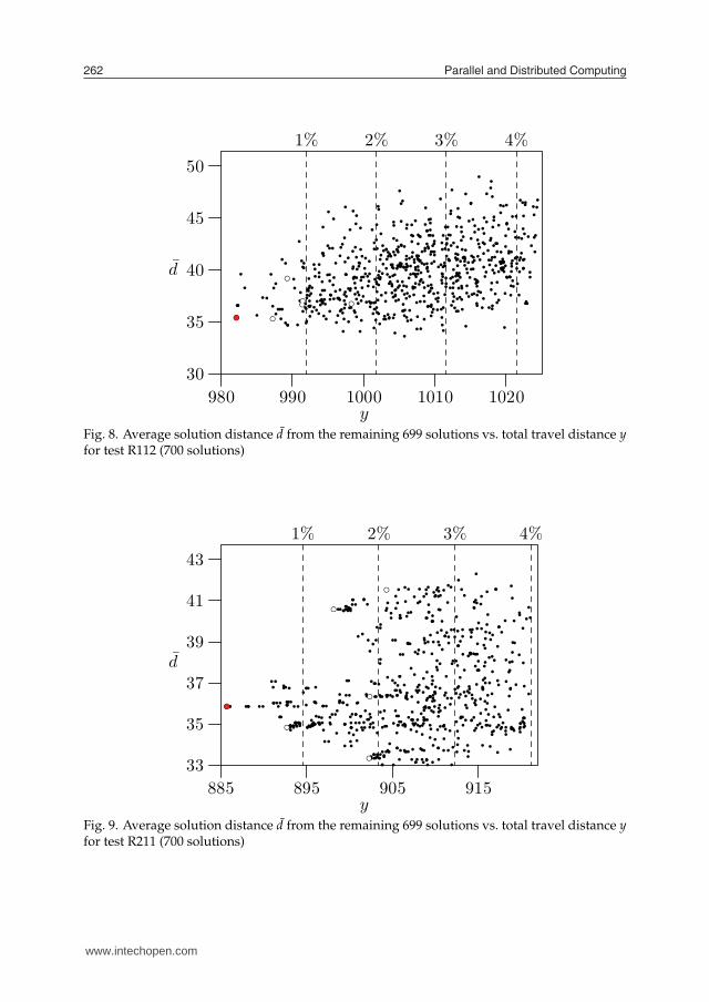
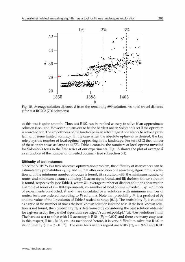
Several experimental studies in discrete optimization revealed correlations among locationsof local optima which suggest existence of a globally convex or “big valley” structures in thefitness landscapes (7). The experiments indicated that local optima are closer (in terms ofdistance d) to the global optimum than are random points in a search space. The local optimaare also closer to each other and form a “big valley” structure with the best local (or global)optimum appearing in a center of the valley. The phenomenon can be illustrated by plotting agraph of fitness against average distance from all other optima. The graph in Fig. 8 shows thatthe best solution (marked by a shaded circle) has almost minimum distance d what implies itis located near the center of the valley. However this is not the case for the graphs in Figs. 9and 10 where many local optima are much closer to the center than the best solution.

Approximate and exact solutions

Suppose that a hard optimization problem is to be solved. Then getting an approximatesolution worse no more than by 0-1% with respect to the optimum can be considered asadequate. In such circumstances a good indicator of the problem difficulty is the value ofτ = (y − ymin)/ymin which exhibits the shift of the average cost y of solutions from ymin at-tained by solving the problem repeatedly. The value of τmax = (ymax − ymin)/ymin providessome insight into the depth of local optima. If τ ≤ 1% is observed then a problem can bethought of as easy to solve. Assuming that 1% accuracy of solution approximation is accept-able, all VRPTW tests, except R112, R110, R108, R211, R207, R210 and RC202, can be classifiedas easy10 (Table 3). Fig. 11 drawn for test R102 shows that all its 700 best solutions found,have their y values within 0.28% margin from ymin, what indicates that the fitness landscape

10 Remembering of course that they are instances of the NP-hard problem being solved by the advancedparallel algorithm.

www.intechopen.com


980 990 1000 1010 1020

30

35

40

45

50

1% 2% 3% 4%

y

d

Fig. 8. Average solution distance d from the remaining 699 solutions vs. total travel distance yfor test R112 (700 solutions)

885 895 905 915

33

35

37

39

41

43

1% 2% 3% 4%

y

d

Fig. 9. Average solution distance d from the remaining 699 solutions vs. total travel distance yfor test R211 (700 solutions)

www.intechopen.com


1365 1385 1405

20

28

36

44

52

1% 2% 3%

y

d

Fig. 10. Average solution distance d from the remaining 699 solutions vs. total travel distancey for test RC202 (700 solutions)

ot this test is quite smooth. Thus test R102 can be ranked as easy to solve if an approximatesolution is sought. However it turns out to be the hardest one in Solomon’s set if the optimumis searched for. The smoothness of the landscape is an advantage if one wants to solve a prob-lem with some limited accuracy. In the case when the absolute optimum is desired, the keyrole plays the number of local optima ν appearing in the landscape. For test R102 the numberof these optima was as large as 44773. Table 4 contains the numbers of local optima unveiledfor Solomon’s tests in the first series of our experiments. Fig. 15 shows the plot of average Kas a function of the number of unveiled optima ν (see subsection 5.1).

Difficulty of test instances

Since the VRPTW is a two-objective optimization problem, the difficulty of its instances can beestimated by probabilities P1, P2 and P3 that after execution of a searching algorithm i) a solu-tion with the minimum number of routes is found, ii) a solution with the minimum number ofroutes and minimum distance allowing 1% accuracy is found, and iii) the best-known solutionis found, respectively (see Table 4, where K – average number of distinct solutions observed ina sample of series of r = 100 experiments, ν – number of local optima unveiled; Exp. – numberof experiments conducted; K and ν are calculated over solutions with minimum number ofroutes; tests are ordered according to P2 column). Note that probability P2 is a product of P1

and the value of the 1st column of Table 3 scaled to range [0,1]. The probability P3 is countedas a ratio of the number of times the best-known solution is found to ν. If the best-known solu-tion is not found, then probability P3 is determined by considering the best solution obtainedfor a given test by the parallel algorithm, see http://sun.aei.polsl.pl/˜zjc/best-solutions.html.The hardest test to solve with 1% accuracy is R104 (P2 = 0.002) and there are many easy testsin this respect, R101, R102, etc. As mentioned before, it is very difficult to solve test R102 toits optimality (P3 = 2 · 10−5). The easy tests in this regard are R205 (P3 = 0.997) and R105

www.intechopen.com


1486 1488 1490

0

5

10

15

20

0.28%

y

d


(P3 = 0.559). As can be seen in Fig. 12 there are many solutions of test R105 located at smalldistances d from the minimum. Clearly, such a dense distribution of good quality solutionssurrounding the optimum one, facilitates the gradual improvements of the configuration of acurrent solution during the process of simulated annealing. In contrast, there are not manyneighbor solutions close to the minima for tests R112, R211, RC202 and R102 (see Figs. 5-7 andFig. 11). Each of these minima belongs to a “small valley” of solutions which occurs awayfrom the “big valley” structure. As the result, reaching those minima from an arbitrary initialsolution by a process of small enhancements is not easy, and sometimes not possible at all.The plots in Fig. 13 and 14 show the difficulty of 39 tests by Solomon. For the tests: R104,R112, RC101, RC105, RC106, both probabilities (P1, P2 in Fig. 13, and P1, P3 in Fig. 14) are lessthan 0.5. Thus these tests can be classified as the most difficult to solve in Solomon’s set.

Taking advantage of landscape properties

In this paragraph we ponder how the features of the fitness landscape can be exploited toimprove the performance of the parallel simulated annealing algorithm solving the VRPTWproblem. Boese et al. (7) proposed an adaptive multi-start algorithm for the traveling salesmanproblem. It consists of two phases. In the first, initial phase, a set of R random local minimais computed. In the second phase, which is executed a specified number of times, based onthe k (k ≤ R) best local minima found so far, an adaptive starting solution is constructed. Thissolution is then improved A times using the greedy descent algorithm, what results in a setof k + A local minima. From this set, the k best minima are selected, a new adaptive startingsolution is formed, and the second phase is repeated. An adaptive starting solution is created

www.intechopen.com


1375 1380 1385

0

10

20

30

40

0.6%

y

d


5 8

26

R104R112

RC106

RC101

RC105

R101 ,R102 ,...

0 0.2 0.4 0.6 0.8 1

0

0.2

0.4

0.6

0.8

1

P1

P2

Fig. 13. Difficulty of tests measured by probabilities P1 and P2 (1% approximate solution isdesired)

www.intechopen.com


5 32

2

R104R112

RC106

RC101

RC105

R205

R105

0 0.2 0.4 0.6 0.8 1

0

0.2

0.4

0.6

0.8

1

P1

P3

Fig. 14. Difficulty of tests measured by probabilities P1 and P3 (best solution is desired)

R102

0 104

2×104

3×104

4×104

0

20

40

60

80

100

K

Fig. 15. Average number of distinct solutions K observed in a sample of series of r = 100experiments vs. number of unveiled local optima ν for 39 Solomon’s tests (for reference, solidline plots Eq. 14)

www.intechopen.com


Test P1 P2 P3 K ν Exp.

R104 0.003 0.002 0.001 12.00 15 41600

R112 0.065 0.011 7 · 10−4 87.00 399 9200R110 0.579 0.259 0.102 60.91 5486 60600R108 0.940 0.442 0.008 95.20 2971 4900R111 0.654 0.472 0.078 65.73 4106 38700R109 0.703 0.492 0.195 30.61 2435 61400R107 0.926 0.566 0.017 80.67 4705 19400

R103 0.909 0.873 2 · 10−4 98.83 3384 4500R106 1.000 0.908 0.008 90.57 17523 72200R105 1.000 0.999 0.559 14.40 185 9100R101 1.000 1.000 0.006 95.41 12488 56000R102 1.000 1.000 2 · 10−5 99.98 44773 48600

R211 0.939 0.071 0.013 71.07 1028 4700R207 0.989 0.249 0.084 78.44 5420 23300R210 1.000 0.416 0.058 70.71 8031 68400R203 1.000 0.559 0.006 96.91 3734 5300R204 1.000 0.745 0.216 48.60 1789 10400R208 1.000 0.769 0.008 75.41 9850 71100R202 1.000 0.878 0.402 39.11 3070 37200R209 1.000 0.970 0.433 21.31 279 4200R206 1.000 0.987 0.049 62.34 854 4400R205 1.000 0.998 0.997 1.28 36 36500R201 1.000 1.000 0.317 10.69 72 4500

RC106 0.195 0.141 0.124 11.68 45 22700RC101 0.336 0.300 0.291 4.91 70 33300RC105 0.357 0.355 0.178 9.00 69 8900RC108 1.000 0.634 0.285 42.60 3192 46800RC104 1.000 0.692 0.031 89.85 15842 40100RC102 0.777 0.743 0.404 11.51 664 76800RC103 1.000 1.000 0.022 46.73 823 17700RC107 1.000 1.000 0.036 4.72 46 15600

RC202 0.948 0.131 0.013 34.55 2387 56000RC203 1.000 0.645 0.043 50.23 2121 25600RC206 1.000 0.890 0.273 10.79 351 27800RC205 1.000 0.911 0.115 22.92 904 42100RC207 1.000 0.937 0.212 8.89 270 22000RC201 1.000 0.958 0.362 12.77 472 50100RC208 1.000 0.971 0.014 13.06 401 18700RC204 1.000 0.999 0.022 28.86 538 68300

Table 4. Selected statistical measures of fitness landscapes P1 – probability that solution hasminimum number of routes, P2 – probability that solution has minimum number of routesand minimum distance allowing 1% accuracy, P3 – probability that solution is the best-knownor best-achieved, K – average number of distinct solutions observed in a sample of seriesof r = 100 experiments, ν – number of local optima unveiled (K and ν are calculated oversolutions with minimum number of routes; tests are ordered according to P2 column)

www.intechopen.com


out of as many frequently occurring edges within the best local minima (salesman’s tours) aspossible, because it is believed that if the “big valley” structure holds, then very good solutionsare located near other good solutions.Boese et al.’s approach cannot be directly used for the VRPTW problem, since its instancesmay not have the “big valley” structure (see Fig. 9 and 10). Moreover, an initial solution isnot enhanced in simulated annealing into a better local minimum, like in greedy descent.It is rather a starting point for a random walk which ends up at some local optimum. Thecorrelation between the quality of this optimum and the quality of the initial solution wherethe search began is quite weak.However a shape of the fitness landscape provides some insight into the procedure whichfinds the set of neighbors N(X) of a current solution X (see section 3). Figs. 6 and 7 indicatethat the optimum solution can be a member of a “small valley” of solutions whose distancesfrom all other solutions—measured by d—are large. Therefore in order to reach any solutionin such an isolated “valley”, the procedure finding the neighbors should create them throughdeep modifications of a current solution. This gives some guarantee that both close and distantneighbors will be constructed with equal probability.The information concerning the ruggedness of the fitness landscape is used to establish theinitial temperature of annealing in our parallel algorithm, what is a standard practice. Sincethe algorithm consists of two phases, the temperature T0, f is computed at the beginning ofeach phase ( f = 1,2). The procedure finding a neighbor solution is executed a specified num-ber of times and the average increase of solution cost ∆ is computed. The initial temperatureT0, f is fixed in such a way that the probability of worsening the solution cost by ∆ in the first

annealing step: e−∆/T0, f , is not larger than a predefined constant—in our case 0.01 (15). If thisprobability is too large then the convergence of simulated annealing is slow.

6. Concluding remarks

The fitness landscape is a useful notion in discrete optimization. It increases the understand-ing of processes which happen during optimization and helps to improve the performanceof optimization algorithms. The experiments conducted for the VRPTW benchmarking testsby Solomon showed that the optimum solution can be located inside a “small valley” placedfar away from the “big valley” containing the predominant number of solutions. In order tobe able to find such an optimum one should assure that among the neighbors of a currentsolution built during an optimization process, there are not only the close neighbor solutionsbut also the distant ones. At the beginning of the process of simulated annealing the initialvalue of the temperature has to be fixed. It is usually done by taking into account the degreeof ruggedness of the fitness landscape of a problem instance being solved. Statistical mea-sures of the fitness landscape can be helpful in establishing the difficulty of instances of theproblem. The analysis of this difficulty has several facets. One may ask how hard is to findthe exact solution to the problem. In this case the key role plays the number of local optimaoccurring in the landscape. This number can be estimated by detecting distinct solutions ina series of experiments. The larger is the numer of these solutions, the more local optimaare present in the landscape, and the problem instance is harder to solve. If one wants tosolve the problem with some accuracy, then the smoothness of the landscape is crucial. Anindicator here can be the value of τ = (y − ymin)/ymin which exhibits the shift of the averagecost y of solutions from ymin attained by solving the problem repeatedly. For two-objectiveminimization problems, like the VRPTW, one can ask what are the probabilities that in a finalsolution produced by an optimization algorithm both objective functions are minimized, or

www.intechopen.com


stay within some accuracy limits. For example, we found that among the VRPTW tests theseprobabilities are the smallest for test R104, and the largest for test R205. Last but not least,the amenability of the problem and its instances for parallelization can be investigated. If thesimulated annealing paradigm is used, then shortening the parallel execution time in order toget speedup, decreases the chains of steps of free exploration of the solution space carried outby processes. However short chains cause deterioration of quality of search results, becausethe convergence of simulated annealing is relatively slow. This difficulty can be alleviatedby making processes co-operate. For this goal a suitable scheme of co-operation and its fre-quency are to be devised. It follows from our experiments that solving most of the VRPTWtests can be accelerated by using up to 20 processes. However for some tests (group III, seesubsection 4.2) solutions of best accuracy are obtained for less than 20 processes. We believethat this issue requires further investigation.

7. Acknowledgments

We thank the following computing centers where the computations of our project were carriedout: Academic Computer Centre in Gdansk TASK, Academic Computer Centre CYFRONETAGH, Krakow (computing grants 027/2004 and 069/2004), Poznan Supercomputing and Net-working Center, Interdisciplinary Centre for Mathematical and Computational Modelling,Warsaw University (computing grant G27-9), Wrocław Centre for Networking and Supercom-puting (computing grant 04/97). The research of this project was supported by the Ministerof Science and Higher Education grant No 3177/B/T02/2008/35.

8. References

[1] Aarts, E.H.L., and Korst, J.H.M., Simulated annealing and Boltzmann machines, Wiley,Chichester, 1989.

[2] Aarts, E.H.L., and van Laarhoven, P.J.M., Simulated annealing: Theory and applications,Wiley, New York, 1987.

[3] Abramson, D., Constructing school timetables using simulated annealing: sequential andparallel algorithms, Man. Sci. 37, (1991), 98–113.

[4] Arbelaitz, O., Rodriguez, C., and Zamakola, I., Low cost parallel solutions for theVRPTW optimization problem, Proceedings of the International Conference on ParallelProcessing Workshops, (2001).

[5] Azencott, R., Parallel simulated annealing: An overview of basic techniques, in Azencott,R. (Ed.), Simulated annealing. Parallelization techniques, J. Wiley, NY, (1992), 37–46.

[6] Azencott, R., and Graffigne, C., Parallel annealing by periodically interacting multiplesearches: Acceleration rates, In: Azencott, R. (Ed.), Simulated annealing. Parallelizationtechniques, J. Wiley, NY, (1992), 81–90.

[7] K. D. Boese, A. B. Kahng, and S. Muddu, A new multi-start technique for combinatorialglobal optimization, Operations Research Letters 16, (1994), 101–113.

[8] Boissin, N., and Lutton, J.-L., A parallel simulated annealing algorithm, Parallel Com-puting 19, (1993), 859–872.

[9] Catoni, O., Grandes deviations et decroissance de la temperature dans les algorithmes derecuit simule, C. R. Ac. Sci. Paris, Ser. I, 307 (1988), 535-538.

[10] Cerny, V., A thermodynamical approach to the travelling salesman problem: an efficientsimulation algorithm, J. of Optimization Theory and Applic. 45, (1985), 41-55.

www.intechopen.com


[11] Czech, Z.J., and Czarnas, P., A parallel simulated annealing for the vehicle routing prob-lem with time windows, Proc. 10th Euromicro Workshop on Parallel, Distributed andNetwork-based Processing, Canary Islands, Spain, (January, 2002), 376–383.

[12] Czarnas, P., Czech, Z.J.,and Gocyla, P., Parallel simulated annealing for bicriterion op-timization problems, Proc. of the 5th International Conference on Parallel Processingand Applied Mathematics (PPAM 2003), (September 7–10, 2003), Czestochowa, Poland,Springer LNCS 3019/2004, 233–240.

[13] Czech, Z.J., and Wieczorek, B., Solving bicriterion optimization problems by parallel sim-ulated annealing, Proc. of the 14th Euromicro Conference on Parallel, Distributed andNetwork-based Processing, (February 15–17, 2006), Montbeliard-Sochaux, France, 7–14(IEEE Conference Publishing Services).

[14] Czech, Z.J., and Wieczorek, B., Frequency of co-operation of parallel simulated annealingprocesses, Proc. of the 6th Intern. Conf. on Parallel Processing and Applied Mathematics(PPAM 2005), (September 11–14, 2005), Poznan, Poland, Springer LNCS 3911/2006, 43–50.

[15] Czech, Z.J., Speeding up sequential annealing by parallelization, Proc. of the Inter-national Conference on Parallel Computing in Electrical Engineering, PARELEC 2006,(September 13–17, 2006), Bialystok, Poland, 349–354 (IEEE Conference Publishing Ser-vices).

[16] Czech, Z.J., Co-operation of processes in parallel simulated annealing, Proc. of the 18thIASTED International Conference on Parallel and Distributed Computing and Systems(PDCS 2007), (November 13-15, 2006), Dallas, Texas, USA, 401–406.

[17] Debudaj-Grabysz, A., and Czech, Z.J., Theoretical and practical issues of parallel sim-ulated annealing, Proc. of the 7th Intern. Conf. on Parallel Processing and AppliedMathematics (PPAM 2007), (September 9–12, 2007), Gdansk, Poland, Springer LNCS4967/2008, 189–198.

[18] Czech, Z.J., Statistical measures of a fitness landscape for the vehicle routing problem,Proc. of the 22nd IEEE International Parallel and Distributed Symposium (IPDPS 2008),11th Intern. Workshop on Nature Inspired Distributed Computing (NIDISC 2008), (April14–18, 2008), Miami, Florida, USA, 1–8.

[19] Czech, Z. J., Mikanik, W., and Skinderowicz, R., Implementing a parallel simulated an-nealing algorithm, (2009), 1–11 (submitted).

[20] Greening, D.R., Parallel simulated annealing techniques, Physica D 42, (1990), 293–306.[21] Hajek, B., Cooling schedules for optimal annealing, Mathematics of Operations Research

13, 2, (1988), 311–329.[22] W. Hordijk and P. F. Stadler, Amplitude spectra of fitness landscapes, J. Complex Systems

1, (1998), 39–66.[23] Kirkpatrick, S., Gellat, C.D., and Vecchi, M.P., Optimization by simulated annealing, Sci-

ence 220, (1983), 671-680.[24] Lenstra, J., and Rinnooy Kan, A., Complexity of vehicle routing and scheduling prob-

lems, Networks 11, (1981), 221–227.[25] Metropolis, N., Rosenbluth, A.W., Rosenbluth, M.N., Teller, A.H., and Teller, E., Equation

of state calculation by fast computing machines, Journ. of Chem. Phys. 21, (1953), 1087-1091.

[26] Onbasoglu, E.,and Ozdamar, L., Parallel simulated annealing algorithms in global opti-mization, Journal of Global Optimization 19: 27–50, 2001.

www.intechopen.com


[27] Reeves, C.R., (Ed.) Modern Heuristic Techniques for Combinatorial Problems, McGraw-Hill, London, 1995.

[28] Reeves, C. R., Direct statistical estimation of GA landscape properties, in: Foundationsof Genetic Algorithms 6, FOGA 2000, Martin, W. N., Spears, W. M. (Eds.), Morgan Kauf-mann Publishers, (2000), 91–107.

[29] Reeves, C. R. and Rowe, J. E., Genetic algorithms: Principles and Perspective. A Guideto GA Theory, Kluwer Academic Publishers, (2003), 231–263.

[30] C. R. Reeves, Fitness landscapes, In: Search methodologies. Introductory Tutorials inOptimization and Decision Support Techniques, Burke, E. K. and Kendall, G. (Eds.), 587–610, Springer-Verlag, Berlin, (2005).

[31] C. M. Reidys and P. F. Stadler, Combinatorial landscapes, SIAM Rev. 44, (2002), 3–54.[32] P. F. Stadler, Towards a theory of landscapes, In: Complex Systems and Binary Networks,

Lopez-Pena, R., Capovilla, R., Garcıa-Pelayo, R., Waelbroeck, H., and Zurteche, F. (Eds.),77–163, Springer-Verlag, Berlin, (1995).

[33] Solomon, M.M., Algorithms for the vehicle routing and scheduling problemswith time window constraints, Operations Research 35, (1987), 254–265, see alsohttp://w.cba.neu.edu/˜msolomon/problems.htm.

[34] Toth, P., and Vigo, D., (Eds.), The vehicle routing problem, SIAM Monographs on Dis-crete Mathematics and Applications, Philadelphia, PA, 2002.

[35] Verhoeven, M.G.A., and Aarts, E.H.L., Parallel local search techniques, Journal of Heuris-tics 1, (1996), 43–65.

[36] Weinberger, E. D., Correlated and uncorrelated landscapes and how to tell the difference,Biol. Cybernet. 63, (1990), 325–336.

[37] S. Wright, The role of mutation, inbreeding, crossbreeding and selection in evolution, In:6th Int. Congress on Genetics 1, Jones, D. (Ed.), (1932), 356–366.

www.intechopen.com


www.intechopen.com

Parallel and Distributed ComputingEdited by Alberto Ros

ISBN 978-953-307-057-5Hard cover, 290 pagesPublisher InTechPublished online 01, January, 2010Published in print edition January, 2010

InTech EuropeUniversity Campus STeP Ri Slavka Krautzeka 83/A 51000 Rijeka, Croatia Phone: +385 (51) 770 447 Fax: +385 (51) 686 166www.intechopen.com

InTech ChinaUnit 405, Office Block, Hotel Equatorial Shanghai No.65, Yan An Road (West), Shanghai, 200040, China

Phone: +86-21-62489820 Fax: +86-21-62489821

The 14 chapters presented in this book cover a wide variety of representative works ranging from hardwaredesign to application development. Particularly, the topics that are addressed are programmable andreconfigurable devices and systems, dependability of GPUs (General Purpose Units), network topologies,cache coherence protocols, resource allocation, scheduling algorithms, peertopeer networks, largescalenetwork simulation, and parallel routines and algorithms. In this way, the articles included in this bookconstitute an excellent reference for engineers and researchers who have particular interests in each of thesetopics in parallel and distributed computing.

How to referenceIn order to correctly reference this scholarly work, feel free to copy and paste the following:

Zbigniew J. Czech (2010). A Parallel Simulated Annealing Algorithm as a Tool for Fitness LandscapesExploration, Parallel and Distributed Computing, Alberto Ros (Ed.), ISBN: 978-953-307-057-5, InTech,Available from: http://www.intechopen.com/books/parallel-and-distributed-computing/a-parallel-simulated-annealing-algorithm-as-a-tool-for-fitness-landscapes-exploration

a parallel simulated annealing algorithm zbigniew j. …cdn.intechweb.org/pdfs/10764.pdf · a...

Documents