HEFAT2014

10th

International Conference on Heat Transfer, Fluid Mechanics and Thermodynamics

14 – 26 July 2014

Orlando, Florida

A NOVEL MATHEMATICAL MODEL AND NUMERICAL SIMULATION OF MASS

AND HEAT TRANSFER IN BIOLEACHING PROCESS OF COPPER

AGGLOMERATE.

Zambra C.E.* and Muñoz J.F. **

*Author for correspondence

*Centro de Estudios en Alimentos Procesados (CEAP), CONICYT-Regional, GORE-Maule, R09I2001,

San Miguel 3425,

Talca, 3460000,

Chile,

E-mail: carlos.zambra.s@gmail.com

**Pontificia Universidad Católica de Chile,

Av. Vicuña Mackena 4860, Macul,

Santiago, 8320000,

Chile,

E-mail: jfmunoz@ing.puc.cl

ABSTRACT

The bioleaching unlike the leaching is a process catalyzed

by bacteria to obtain copper. Generally, the material containing

copper is previously agglomerated to build piles. A three

dimensional mathematical model to describe the fluid

mechanics, mass and heat transport that consider source terms

for oxidation reaction, biological kinetic, and oxygen depletion

due to methanogenic bacteria (15-45 ºC), is presented. The

results of computational simulations made with original

programs using the proposed mathematical model, the finite

volume method and RECT computational package were

validated comparing it with experimental results obtained from

a leaching pile of tailing agglomerated. These shown good

concordances between them. When the effect of the catalyzing

bacteria was included, is possible to predict their effect over the

temperature, oxygen concentration and acid consume for a pile

with bioleaching process.

INTRODUCTION The bioleaching is a leaching process catalyzed by

microorganisms and applied to copper sulfate minerals to

improve the dissolution kinetic. The bacteria involved in the

process are generally autotrophic, aerobic and chemosynthetic

and resistant to extreme acid and high metal concentration

media. The copper extraction from minerals such as chalcocite

(Cu2S) and covellite (CuS) by bioleaching is practiced

commonly in mines around the world. The thermophilic

bacteria are the most studied due to the advantages in

biohydrometallurgy processes. In order to reach maximum

copper recuperation from the pile 80-90%, is required 250-350

days of process [1]. The oxidation reactions are exothermic and

allow self-heating the pile which improves the copper

recuperation.

A mathematical model for the self-heating in piled material

has been introduced by Sidhu et al. [2] and using by same

authors [3-5] to predict with finite volume numerical

simulations the self-heating in compost pile. This model has the

particularity of group the effect of the growth of

microorganisms colony in an parametrized equation,

comparatively simple in front of classical equations of biologic

kinetic. The oxidation reaction of the organic matter may be

describe by and Arrhenius type equation [2]. In order to predict

the solute flow in soil is used an equation that considers the

advection (Darcy law), diffusion (Fick law) and hydrodynamic

dispersion. This equation consider that solute is diluted in water

thus is flowing with it [6].

In this paper is proposed a mathematical model for the

oxygen flow, energy and acid solution inside of copper

bioleaching pile located in field. The three dimensional

mathematical model is solved with the finite volume method

[7]. Numerical results with analytical solution and Numerical

results with experimental data are compared in order to validate

the algorithm accuracy. The results show that is possible to

predict the solute flow and the water transport with errors less

than 5%. The three dimensional simulation describe the internal

distribution of the variables; water temperature increases,

oxygen and acid consume.

1362

NOMENCLATURE A1 [1/s] Pre-exponential factor for the oxidation

A2 [-] Pre-exponential factor for the inhibition of biomass

growth C [kg/m3] Concentration

,p TC [J/kgK] Coefficient dependent on geometric, thermal and

material property values D [m2/s] Diffusion coefficient.

E [J/mol] Activation energy

k [W/mK] Thermal conductivity h [m] Head pressure

K [cell/l] Cell crowding

Kd [m3/kg] Distribution coefficient '''G [W/m3] Volumetric heat generation density

R [J/K mol] Ideal gas constant Rf [-] Retardation factor

t [d] time

T [K] Temperature S [-] Source term

x [m] Cartesian axis direction

y [m] Cartesian axis direction z [m] Cartesian axis direction

Special characters

[kg/m3] Density

,s b [kg/m3] Bulk density

[-] Volumetric water content

f [-] Function

[1/s] Reaction velocity

[m] Tortuosity

ε [-] Porosity

[kg/m3d] Dispersivity

[m/d] Porous mean velocity

[-] Variable

δ [-] First order degradation constant

Subscripts

b biomass T Temperature

eff Volumetric effective expression

irr Irrigation mgr Mass growth

fl Fluid phase

ox Oxygen max Maximum

m Mass

s Sulfur Fe ferrous

MATHEMATICAL MODEL For the temperature and oxygen concentration was assumed

that the flow velocity inside the porous media is low, the

convective terms values are very small compared with the

diffusive terms values and hence in these cases the convective

terms may be despised. The mathematical model considers the

diffusion of temperature and oxygen and convection-diffusion

of water and solute in porous media with chemical and

biological reactions [4]. This model assumes that the

microorganisms growth is possible due to ability to consume on

iron and sulfur. The equation (1) shown the model for the

temperature and oxygen

''' '''

, ,

2

p T eff T ox beff

TC k T G G

t

;

'''2oxfl eff ox ox

CD C G

t

(1)

Heat and mass transfer properties in the porous media are

defined in terms of the pile porosityflε ,

( )eff fl air fl mk k 1 k ;

, , ,( )p T fl air p air fl m p meffC C 1 C ;

,eff fl air mD D (2)

In these equations Gb’’’

,Ge,ox’’’

, are the generations caused by

biomass growth and the chemical reactions, and -Gox’’’

, is the

oxygen consume due to chemical reaction and temperature

increases. The generation and consume terms are characterized

by a reaction velocity ( ).

'''

, , ( )T ox T ox fl m ox moxG Q 1 C ; ''' ( )b b fl b ox mgrG Q 1 F ;

oxE

RT

mox oxA e

(3)

Here, mox , is and Arrhenius type equation used to describe

the oxidation velocity due to chemical reaction and mgr is the

velocity of the reactions catalyzed by microorganisms. In the

present model was assumed that bacteria that consume iron and

sulfur are the main cause of the self-heating. The microbial

growth rate is expressed as a maximum microbial growth

modified by limiting factors. The growth rate of iron oxidizing

microbes is given by

max

,max ( )[ ]

H

2H

2 2

2

C

CFe

Fe Fe

Fe Fe

ox I

ox ox I Fe

Cf T 1 e

K C

C K

K C K N

. (4)

This equation shows a dependence of the growth rate of iron

oxidizing microbes on temperature ( )f T , pH (H

C ), ferrous ion

concentration (2Fe

C ), oxygen concentration (

oxC ), and cell

crowding (IK ). A similar expression is written for the growth

rate of sulfur oxidizing microbes. Sulfur oxidizing microbes

grow by oxidizing elemental sulfur at the surface of the ore

particles. Therefore, it will be assumed that planktonic sulfur

oxidizers do not grow. The growth rate of adsorbed sulfur

oxidizers is given by

,max ( ) S ox IS S

S S ox ox I S

g C Kf T

K g K C K N

(5)

In this article we propose a parametrized equation to

describe the metabolic activity of biomass.

( )

1

2

E

RT

1

E

RT

2

A ef T

1 A e

(6)

1363

The formulation of equation (6) encapsulates that activation

and inactivation processes occur over different temperature

ranges. At low temperatures the metabolic activity of the

biomass grows with increasing temperature. These processes

are governed by the parameters A1 and E1. Equation (6) can be

derived theoretically by assuming that the biomass growth rate

is determined by a rate limiting step in which there is an

equilibrium between “activated” and “unactivated” forms of the

biomass [8]. From this, thermodynamic, perspective the term A2

exp(−E2/RT ) represents the temperature dependence of the

equilibrium constant whilst the expression A1 exp(−E1/RT) is

the maximum forward rate of reaction in the rate limiting step.

Roels [8], notes that “Although this model is based on a highly

simplified image of the complexity of the growth process, it can

be considered an efficient tool to model the temperature

dependence of the maximum rate of growth”. Eq. (6) has been

used to model the maximum specific biomass growth rate in the

aerobic biodegradation of the organic fraction of municipal

solid waste [9]. It has also been used in a number of models for

solid-state fermentation processes [10-13]. Finally, the total

microbial growth rate for the mesophilic microorganisms in the

bioleaching pile is obtained

mgr Fe s (7)

This expression was incorporated in equation (3) for the

heat generation by biomass growth.

The solute transfer in soil is calculated with an equation that

considers advection, diffusion and hydrodynamic dispersion in

porous media with chemical reactions.

,

,

,

,

( )[ ]

( )[ ]

[ ]

s s b se y

w s se x

se z

C s CD

t y y

J C CD

y x x

CD S

z z

(8)

; ( ) ; ( ) ;

; ;

7

3s s w

e l lh l 1 l 1 2

s

wlh w s

D D D D D

J HD J K

y

(9)

Here, Cs is the soil solute concentration, b,sρ the bulk

density, s soil solute absorption, , , ,, ,e x e y e zD D D , are the

solute effective dispersion coefficient of soil in x,y,z coordinate

respectively, s

lD the solute effective diffusion coefficient in

soil, )θ(ξ1 is the tortuosity,

w

lD solute diffusion coefficient in

free water, lhD is the hydrodynamic dispersion coefficient, ν

water mean velocity in the porous, λ is the dispersivity, wJ is

the Darcy flux, H is the water head potential (H = h + y) in the

soil, Ks is the saturated hydraulic conductivity and S is the

source term. If an equilibrium lineal adsorption is considered:

sdCKs= , (10)

where dK is the distribution coefficient corresponding to the

slope of adsorption isotherm. When the assumption of linear

absorption and water flow in steady state in soil are considered,

the equation (8) turns to [6]:

2 2

, ,

2

,

s s s sf e y e x2 2

se z f s2

C C C CR D D

t y y x

CD R C

z

(11)

θ

Kρ1R

db,s

f += , (12)

where Rf is the unit-less retardation factor and δ is a first-

order degradation constant. The dependence of the solute

parameter w

lD anddK on the temperature is calculated

through the follows equation [14].

ref

refp

RTT

)TT(E

exp)T(f = , (13)

where Ep , is the activation energy of the process being modeled,

R is the universal gas constant, and Tref (293.15 K or 20 ºC) is

the reference temperature for optimal production.

The Richards equation is commonly used to describe the

water transfer in soils.

( )[ ( ) ( )]

[ ( ) ] [ ( ) ]

y

x z

h hK h K h

t y y

h hK h K h

x x z z

(14)

Here, θ is the water content, h the hydraulic pressure, K(h)x,

K(h)y and K(h)z, are the hydraulic conductivity in x,y,z

coordinate respectively. When the water content in the soil is

either steady state or saturated with water, the gradients in

equation (14) are zero and the water content value in the

domain is known. The van Genuchten model [15] for the

variation of water content with the hydraulic pressure was used

in all cases.

NUMERICAL METHOD

The system of equations that governs this problem (1, 12

and 14) was solved numerically using the finite volume

method, Patankar [7]. Each one of the governing equations was

written in the general form of the transport equation, with

unsteady, diffusion and linearized source terms:

SpScgraddiv

t (15)

A first-order accuracy in time was used in the numerical

scheme to account for the unsteady heat and mass terms

tt

ttt

(16)

The diffusion coefficient ( ) and source terms (Sc, Sp) for

each dependent variable are given in Table 1.

An original computational program, written in Fortran

language, with a combination of the TDMA and Gauss-Seidel

1364

method an iterative solver [7] was used to predict temperature

and oxygen concentration inside the compost pile.

The pile geometry was discretized using uniform grid of:

40x26x40 nodes in the x,y,z directions, respectively, to verify

that the results obtained were not influenced by the mesh size.

Numerical simulations were carried out for pile: 50x22x5.5 m

of width, large and height.

Temperature increases initially smoothly while oxygen

decreased slowly with time until sudden changes, caused by the

material heat generation. Therefore, a strategy based on the use

of dynamic time steps was implemented, with lower time steps

when the unsteady terms were higher. The different values of

the time steps used in the unsteady calculations were in the

interval.

600s Δt 86400s (17)

The iterative procedure ends at each time step when the

maximum difference between iteration for , ,ox sT C C ,

satisfied in each control volume the convergence criteria 4

,

1

, 10 k

ji

k

ji (18)

Table 1. Diffusion coefficients and source terms for the waste

pile mathematical model.

VALIDATION AND NUMERICAL CASES

Water flow in experimental leaching pile

In this section the experimental results obtained from

agglomerated tailing material are compared with numerical

results.

The experimental procedure is explained below. The tailing

material with humidity of 13.2% (p/p), was agglomerated using

22.62 kg of sulfuric acid and 11.7 l of refining solution by ton

of dry material. The product is an agglomerated material with

final humidity of 14.4% (p/p). This material was disposal in a

field pile of size 50mx22mx5.5m large, wide and high,

respectively with lateral slopes of 45º. An impermeable carpet

with drainage tubes were placed in the pile base. The bulk

density of the piled material was 1550 kg/m3.

The pile was drip irrigated on a surface of 308 m2 with

configuration of 1m between tubes and 0.9 m between

droppers. The water average flow was 3.41 L/h m2. In figure 1

is shown the daily volume on the surface.

Figure 1. Water daily volume on the surface of leaching pile

In the final steps of the pile construction, samples of the

piled material each 1m of high from different point along the

pile were taken. These samples were used to observe the

granulometry spatial variation of the material. The results

indicate the formation of two material types. The first is similar

to the sand and the second to pelletized material that was not

agglomerated in the process and seem spheres from 0.01m to

0.08m of diameter with high humidity. These pellets are

distributed mainly in the lower zone of the pile. For this reason

the pile was divided in three horizontal layers. The first is

located in the upper zone and has 1m of thickness. It is

composed by homogeneous mixture of agglomerated material

and pellets. The second layer is located in the intermediate zone

and is composed by 3.5m of agglomerated tailing. The third is a

lower layer of 1m thickness of pellets material. The

hydrodynamics properties were determinate for each layer. In

order to find the experimental suction curve were used pressure

cells with range between 0 to 1 bar. The saturated hydraulic

conductivity was determinate by using of constant head

permeameter. Experimental values of the suction curve and

saturated conductivity are incorporated to the RECT program

[15,16] in order to obtain the van Genuchten parameters for the

water content and unsaturated hydraulic conductivity for each

layer defined in the granulometry study detailed in previous

paragraph. In figure 2 are observed the experimental results and

adjusted curves obtained using the RECT program and the van

Genuchten model [15].

Sc Sp

( )h ( )K h ( )Δ h

Δt

( )ΔK h

Δy

T effk t

T p

+

''' '''

,e ox bG G t

1

oxC effD t

Cp

ox

'''

oxGt

1

sC eD sC

y

+p

f sR C

Δt

fRfR

Δt

1365

Figure 2 Experimental point and suction curves calculated

by RECT for each layer.

The van Genuchten parameters for each layer are shown in

table 2.

Table 2. Van Genuchten parameters obtained with RECT

program for each layer.

Parameters upper layer middle layer lower layer

r (m3/m

3) 0 0 0.140

s (m3/m

3) 0.325 0.330 0.407

(1/d) 3.023 1.368 7.060

N 1.265 1.411 1.200

M 0.209 0.292 0.167

L 0.500 0.5 0.5

Ks (m/d) 1.776 1.680 2.141

The time evolution of the water flux in the pile base from

experimental data and numerical simulation are compared after

43d in figure 3. Numerical simulations results are obtained

solving the Richards equation (14). The numerical values are

close to the experimental. Higher difference of q is after 43d

and reaches 0.002 m/d.

Figure 3 Measured and calculated transient values of the

flux at bottom of the pile.

Comparison for the solute transport model

In this section are presented comparisons between analytical

and numerical results for solute transport in soil. Considering

the transport in homogeneous and isotropic porous media,

steady and unidirectional water flow and lineal solute

adsorption, the transport equation (8) becomes: 2 2

2

;

s s s sf L T2 2

sT f s2

C C C CR D D

t y y x

CD R C

z

(19)

;

θ

Kρ1R

db

f +=

s

d C

sK = (20)

where DT y DL are soil dispersion coefficients in y,x,z

coordinates, Rf is the soil retardation factor, Kd is the

distribution coefficient and λ , are the degradation constants

to chemical reaction of zero and first order, respectively. The

analytical solution of equation (19) is [6].

,

( )

/ /

/ /

( )( , , , ) exp

( / ) ( / )

( / ) ( / )

2 2tf fs i

s 3

L f f LP t

1 2 1 2

T f T f

1 2 1 2

T f T f

R z R z vCC x y z t

4 4 D R 4R D

x a x aerfc erfc

2 D R 2 D R

y b y berfc erfc d

2 D R 2 D R

/

/

( )exp

exp( )

f

1 2t

f L

f f0 f

1 2

L f L

v R zerfc

2 R Dd

2R R R z vvzerfc

D 2 R D

(21)

The calculate domain have dimensions of 120m x 200m x

120m and mesh of 88x98x88 nodes in x,y,z direction,

respectively. The time step is 1d. Initially, solute-free medium

is subjected to a source of Cs,i=1kg/m3. The rectangular surface

source has dimensions x=0-50m and z=0-50m at y=200m.

Then, the boundary conditions may be written as:

Cs(x,y,200,t)=Cs,i=1kg/m3 if 0<x<50m or 0<z<50m;

Cs(x,y,200,t)=0 if 50<x<120m or 50<z<120m. The input

transport parameters for simulations are listed in Table 6.

Tabla 6 Input parameters for comparison with analytical

solution

The three dimensional results for solute concentration obtained to

0.1 kg/m3 after 10, 50, 100 and 365 days, are shown in figure 5.

ν

m/d

1/d

kg/m3d

DT

m2/d

DL

m2/d

Rf Cs,i

kg/m3

a

m

b

m

0.1 0.01 0 0.5 1 3 1 52 52

1366

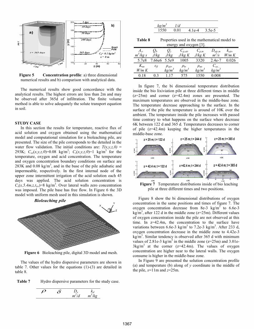
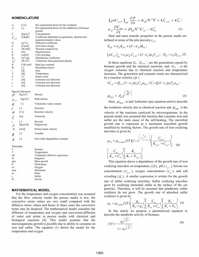
Figure 5 Concentration profile: a) three dimensional

numerical results and b) comparison with analytical data.

The numerical results show good concordance with the

analytical results. The highest errors are less than 2m and may

be observed after 365d of infiltration. The finite volume

method is able to solve adequately the solute transport equation

in soil.

STUDY CASE

In this section the results for temperature, reactive flux of

acid solution and oxygen obtained using the mathematical

model and computational simulation for a bioleaching pile, are

presented. The size of the pile corresponds to the detailed in the

water flow validation. The initial conditions are: T(x,y,z,0) =

293K; Cox(x,y,z,0)=0.08 kg/m3; Cs(x,y,z,0)=1 kg/m

3 for the

temperature, oxygen and acid concentration. The temperature

and oxygen concentration boundary conditions on surface are

283K and 0.08 kg/m3, and in the base of the pile adiabatic and

impermeable, respectively. In the first internal node of the

upper zone intermittent irrigation of the acid solution each 45

days was applied. The acid solution concentration is

Cs(x,5.4m,z,tirr)=8 kg/m3. Over lateral walls zero concentration

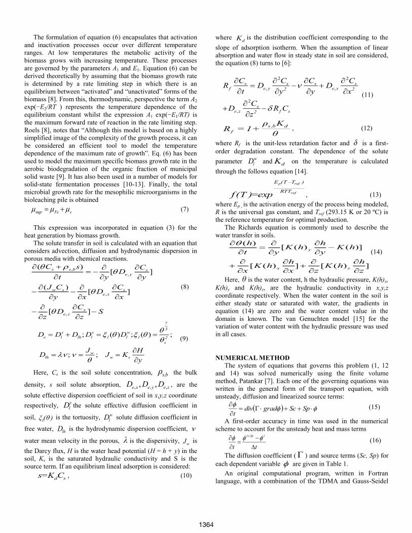
was imposed. The pile base has free flow. In Figure 6 the 3D

model with uniform mesh used in this simulation is shown.

Figure 6 Bioleaching pile, digital 3D model and mesh.

The values of the hydro dispersive parameters are shown in

table 7. Other values for the equations (1)-(3) are detailed in

table 8.

Table 7 Hydro dispersive parameters for the study case.

De

m2/d

kd

m3/kg

kg/m3

1/d

1550 0.01 4.1e-4 3.5e-5

Table 8 Properties used in the mathematical model to

energy and oxygen [3].

Ac,

m3/kg s

Qb

J/kg

Qc

J/kg

Cp,air

J/kg K

Cp,m

J/kg K

Dair,m

m2/s

kair,

W/m K

5.7e8 7.66e6 5.5e9 1005 3320 2.4e-7 0.026

Km,

W/m K

εfl ρair,

kg/m3

ρb,

kg/m3

ρm,

kg/m3

Cox ,

kg/m3

0.18 0.3 1.17 575 1550 0.008

In figure 7, the bi dimensional temperature distribution

inside the bio lixiviation pile at three different times in middle

(z=25m) and corner (z=42.4m) zones are presented. The

maximum temperatures are observed in the middle-base zone.

The temperature decrease approaching to the surface. In the

surface of the pile the temperature is around of 10K over the

ambient. The temperature inside the pile increases with passed

time contrary to what happens on the surface where decrease

6K between 122 d and 365 d. Temperatures decreases to corner

of pile (z=42.4m) keeping the higher temperatures in the

middle-base zone.

Figure 7 Temperature distributions inside of bio leaching

pile at three different times and two positions.

Figure 8 show the bi dimensional distributions of oxygen

concentration in the same positions and times of figure 7. The

oxygen concentration decrease from 8e-3 kg/m3 to 6.6e-3

kg/m3, after 122 d in the middle zone (z=25m). Different values

of oxygen concentration inside the pile are not observed at this

time. In z=42.4m, the concentration to the surface have

variations between 6.6e-3 kg/m3 to 7.2e-3 kg/m

3. After 233 d,

oxygen concentration decrease in the middle zone to 4.42e-3

kg/m3. Similar tendency is observed after 365 d with minimum

values of 2.81e-3 kg/m3 in the middle zone (z=25m) and 3.01e-

3kg/m3

at the corner (z=42.4m). The values of oxygen

concentration are higher near to the lateral walls. The oxygen

consume is higher in the middle-base zone.

In Figure 9 are presented the solution concentration profile

(a) and temperature (b) along of y coordinate in the middle of

the pile, x=11m and z=25m.

Z

XY

Bioleaching pile

305305

304298

304

x (m)

y(m

)

0

2

4

6

8 z = 25 m; t = 122 d

306

304300 296 296

306

x (m)

y(m

)

0

2

4

6

z = 25 m; t = 244 d

307

304302298 294

306

x (m)

y(m

)

0

2

4

6

8 z = 25 m; t = 365 d

305304

302298

300304

x (m)

y(m

)

0

2

4

6

8

z = 42.4 m; t = 122 d

305302300

296 294

304

x (m)

y(m

)

0

2

4

6

8

z =42.4 m; t = 244 d

305

300298294 292

302

x (m)

y(m

)

35 40 45 50 550

2

4

6 z = 42.4 m; t = 365 d

1367

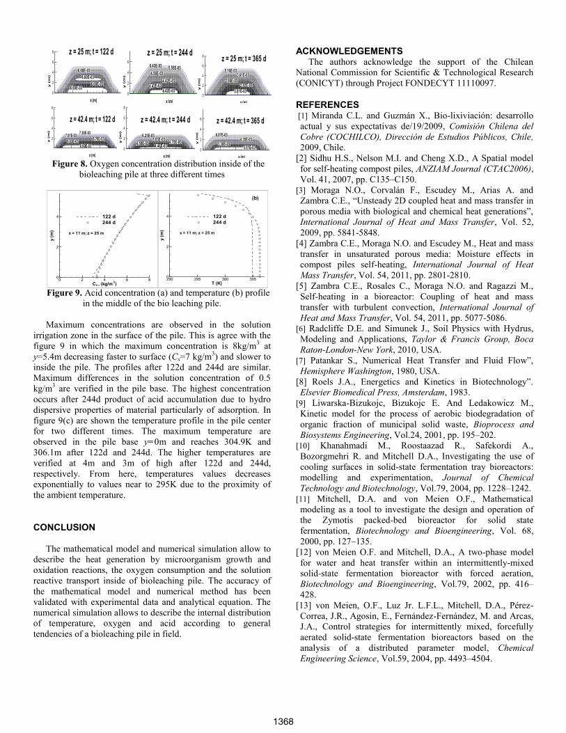
Figure 8. Oxygen concentration distribution inside of the

bioleaching pile at three different times

Figure 9. Acid concentration (a) and temperature (b) profile

in the middle of the bio leaching pile.

Maximum concentrations are observed in the solution

irrigation zone in the surface of the pile. This is agree with the

figure 9 in which the maximum concentration is 8kg/m3 at

y=5.4m decreasing faster to surface (Cs=7 kg/m3) and slower to

inside the pile. The profiles after 122d and 244d are similar.

Maximum differences in the solution concentration of 0.5

kg/m3 are verified in the pile base. The highest concentration

occurs after 244d product of acid accumulation due to hydro

dispersive properties of material particularly of adsorption. In

figure 9(c) are shown the temperature profile in the pile center

for two different times. The maximum temperature are

observed in the pile base y=0m and reaches 304.9K and

306.1m after 122d and 244d. The higher temperatures are

verified at 4m and 3m of high after 122d and 244d,

respectively. From here, temperatures values decreases

exponentially to values near to 295K due to the proximity of

the ambient temperature.

CONCLUSION

The mathematical model and numerical simulation allow to

describe the heat generation by microorganism growth and

oxidation reactions, the oxygen consumption and the solution

reactive transport inside of bioleaching pile. The accuracy of

the mathematical model and numerical method has been

validated with experimental data and analytical equation. The

numerical simulation allows to describe the internal distribution

of temperature, oxygen and acid according to general

tendencies of a bioleaching pile in field.

ACKNOWLEDGEMENTS The authors acknowledge the support of the Chilean

National Commission for Scientific & Technological Research

(CONICYT) through Project FONDECYT 11110097.

REFERENCES [1] Miranda C.L. and Guzmán X., Bio-lixiviación: desarrollo

actual y sus expectativas de/19/2009, Comisión Chilena del

Cobre (COCHILCO), Dirección de Estudios Públicos, Chile,

2009, Chile.

[2] Sidhu H.S., Nelson M.I. and Cheng X.D., A Spatial model

for self-heating compost piles, ANZIAM Journal (CTAC2006),

Vol. 41, 2007, pp. C135–C150.

[3] Moraga N.O., Corvalán F., Escudey M., Arias A. and

Zambra C.E., “Unsteady 2D coupled heat and mass transfer in

porous media with biological and chemical heat generations”,

International Journal of Heat and Mass Transfer, Vol. 52,

2009, pp. 5841-5848.

[4] Zambra C.E., Moraga N.O. and Escudey M., Heat and mass

transfer in unsaturated porous media: Moisture effects in

compost piles self-heating, International Journal of Heat

Mass Transfer, Vol. 54, 2011, pp. 2801-2810.

[5] Zambra C.E., Rosales C., Moraga N.O. and Ragazzi M.,

Self-heating in a bioreactor: Coupling of heat and mass

transfer with turbulent convection, International Journal of

Heat and Mass Transfer, Vol. 54, 2011, pp. 5077-5086.

[6] Radcliffe D.E. and Simunek J., Soil Physics with Hydrus,

Modeling and Applications, Taylor & Francis Group, Boca

Raton-London-New York, 2010, USA.

[7] Patankar S., Numerical Heat Transfer and Fluid Flow”,

Hemisphere Washington, 1980, USA.

[8] Roels J.A., Energetics and Kinetics in Biotechnology”.

Elsevier Biomedical Press, Amsterdam, 1983.

[9] Liwarska-Bizukojc, Bizukojc E. And Ledakowicz M.,

Kinetic model for the process of aerobic biodegradation of

organic fraction of municipal solid waste, Bioprocess and

Biosystems Engineering, Vol.24, 2001, pp. 195–202.

[10] Khanahmadi M., Roostaazad R., Safekordi A.,

Bozorgmehri R. and Mitchell D.A., Investigating the use of

cooling surfaces in solid-state fermentation tray bioreactors:

modelling and experimentation, Journal of Chemical

Technology and Biotechnology, Vol.79, 2004, pp. 1228–1242.

[11] Mitchell, D.A. and von Meien O.F., Mathematical

modeling as a tool to investigate the design and operation of

the Zymotis packed-bed bioreactor for solid state

fermentation, Biotechnology and Bioengineering, Vol. 68,

2000, pp. 127–135.

[12] von Meien O.F. and Mitchell, D.A., A two-phase model

for water and heat transfer within an intermittently-mixed

solid-state fermentation bioreactor with forced aeration,

Biotechnology and Bioengineering, Vol.79, 2002, pp. 416–

428.

[13] von Meien, O.F., Luz Jr. L.F.L., Mitchell, D.A., Pérez-

Correa, J.R., Agosin, E., Fernández-Fernández, M. and Arcas,

J.A., Control strategies for intermittently mixed, forcefully

aerated solid-state fermentation bioreactors based on the

analysis of a distributed parameter model, Chemical

Engineering Science, Vol.59, 2004, pp. 4493–4504.

6.60E-03

6.60E-03

6.60E-036.60E-03

x (m)

y(m

)

0

2

4

6

8 z = 25 m; t = 122 d

6.43E-03 5.55E-034.56E-03

4.42E-034.42E-03

4.42E-03

x (m)

y(m

)

0

2

4

6

z = 25 m; t = 244 d

5.16E-033.61E-03

2.90E-032.82E-03

2.81E-03

x (m)

y(m

)

0

2

4

6

8 z = 25 m; t = 365 d

7.01E-037.20E-03

6.76E-036.63E-03

6.60E-03

x (m)

y(m

)

2

4

6

8

z = 42.4 m; t = 122 d

6.23E-035.03E-03

4.75E-034.58E-034.46E-03

x (m)

y(m

)

0

2

4

6

8

z = 42.4 m; t = 244 d

6.07E-034.35E-03

3.30E-033.01E-03

x (m)

y(m

)

0

2

4

6 z = 42.4 m; t = 365 d

C , (kg/m )

y(m

)

0 2 4 6 80

2

4 122 d

244 d

s3

x = 11 m; z = 25 m

T (K)

y(m

)

290 295 300 3050

2

4 122 d

244 d

x = 11 m; z = 25 m

(b)

1368

[14] Köhne J.M., Köhne S.and Šimůnek J., A review of model

applications for structured soils: a) Water flow and tracer

transport, Journal of Contaminant Hydrology, Vol. 104, 2009,

pp. 4–35.

[15] van Genuchten M. Th., Leij F. J., Yates S. R., The RETC

Code for Quantifying Hydraulic Function of Unsatured Soils,

USEPA Rep. 600/2-91/065. U.S. Salinity Laboratory,

Riverside, CA., 1991, USA.

[16] Yates S., R., van Genuchten M., Th., Warrick A. W. and

Leij F. J., Analysis of Measured, Predicted, and Estimated

Hydraulic Conductivity Using the RETC Computer Program,

Soil Sci. Soc. Am. J., Vol. 56, 1992, pp. 347-354.

1369