MNRAS 000, 1–10 (2017) Preprint 18 October 2017 Compiled using MNRAS LATEX style file v3.0

A new all-sky map of Galactic high-velocity clouds from

the 21-cm HI4PI survey

Tobias Westmeier1⋆

1International Centre for Radio Astronomy Research (ICRAR), The University of Western Australia, 35 Stirling Highway,Crawley WA 6009, Australia

Accepted XXX. Received YYY; in original form ZZZ

ABSTRACT

High-velocity clouds (HVCs) are neutral or ionised gas clouds in the vicinity of theMilky Way that are characterised by high radial velocities inconsistent with partic-ipation in the regular rotation of the Galactic disc. Previous attempts to create ahomogeneous all-sky H I map of HVCs have been hampered by a combination of poorangular resolution, limited surface brightness sensitivity and suboptimal sampling.Here, a new and improved H I map of Galactic HVCs based on the all-sky HI4PIsurvey is presented. The new map is fully sampled and provides significantly betterangular resolution (16.2 versus 36 arcmin) and column density sensitivity (2.3 versus3.7 × 1018 cm−2 at the native resolution) than the previously available LAB survey.The new HVC map resolves many of the major HVC complexes in the sky into anintricate network of narrow H I filaments and clumps that were not previously resolvedby the LAB survey. The resulting sky coverage fraction of high-velocity H I emissionabove a column density level of 2 × 1018 cm−2 is approximately 15 per cent, which re-duces to about 13 per cent when the Magellanic Clouds and other non-HVC emissionare removed. The differential sky coverage fraction as a function of column densityobeys a truncated power law with an exponent of −0.93 and a turnover point at about5×1019 cm−2. H I column density and velocity maps of the HVC sky are made publiclyavailable as FITS images for scientific use by the community.

Key words: ISM: clouds – Galaxy: halo – Galaxy: kinematics and dynamics – radiolines: ISM

1 INTRODUCTION

High-velocity clouds (HVCs) are gas clouds detected in theoptical and ultraviolet, but most notably in the 21-cm lineof neutral hydrogen, across much of the sky at radial veloc-ities that are incompatible with the regular rotation of theGalactic disc. There is no general consensus on how to sep-arate HVCs from gas at low and intermediate velocities. Inthe past, most authors applied a fixed velocity threshold of90 or 100 km s−1 in the Local Standard of Rest (LSR). How-ever, this is clearly insufficient, as Galactic disc emission stilloccupies such extreme velocities in some parts of the sky. Animproved definition was proposed by Wakker (1991) who in-troduced a so-called deviation velocity of vdev = 50 km s−1

to characterise HVCs as deviating by a fixed velocity sepa-ration from the maximally permissible velocity of Galacticdisc emission in a given direction. Today, the concept of de-viation velocity is the most commonly applied criterion for

⋆ E-mail: tobias.westmeier@uwa.edu.au

defining high-velocity gas, although the actual value of vdev

may differ from the one applied by Wakker (1991).

HVCs come in a wide range of sizes and shapesranging from large complexes and streams, such as theMagellanic Stream (Mathewson et al. 1974) or complex C(Hulsbosch 1968), to (ultra-)compact and isolated HVCs(CHVCs/UCHVCs; Braun & Burton 1999; Adams et al.2013). The discovery of 21-cm H I emission from HVCsby Muller et al. (1963) sparked an intense scientific debateabout their spatial distribution and origin (e.g., Oort 1966).This debate was settled only recently when distance brack-ets or upper limits for several HVCs became available, mostnotably halo gas in the direction of the Large MagellanicCloud (Savage & de Boer 1981), complex M (Danly et al.1993), complex A (Wakker et al. 1996; van Woerden et al.1999), complex C (Wakker et al. 2007; Thom et al. 2008),the Cohen Stream (Wakker et al. 2008), complex GCP(Wakker et al. 2008) and complex WD (Peek et al. 2016),confirming that HVCs are generally located several kpcabove the Galactic plane in close proximity to the MilkyWay. This rules out the hypothesis that HVCs are pri-

c© 2017 The Authors

2 T. Westmeier

mordial dark-matter haloes distributed throughout the Lo-cal Group (Blitz et al. 1999), instead suggesting diversegas infall or outflow mechanisms as the origin of mostof the clouds (Cox 1972; Bregman 1980; de Boer 2004;Lehner & Howk 2010; Fraternali et al. 2015; Fox et al. 2016;Marasco & Fraternali 2017). HVCs also contain significantcomponents of ionised gas that can be traced with thehelp of optical and ultra-violet absorption spectroscopy(Sembach et al. 2003; Fox et al. 2006). For a comprehensivereview of the properties and origin of HVCs the reader isreferred to Wakker & van Woerden (1997), Wakker (2001)and van Woerden et al. (2004).

The issue of creating complete all-sky maps of HVCshas been strongly tied to the availability of homogeneous,sensitive, all-sky surveys of Galactic H I emission. An initial,rather patchy all-sky map of HVCs based on the combina-tion of different data sources was presented by Bajaja et al.(1985). The map included data from the IAR 30-m antennaand already showed the general outline of several of thelarge HVC complexes known today, including the MagellanicStream and Leading Arm, complex C and the anti-centrecomplex. A much improved HVC survey of the northern skywith the 25-m Dwingeloo radio telescope was presented byHulsbosch & Wakker (1988). Their map reveals all of thelarge HVC complexes in the northern sky, including com-plexes A, C and M as well as the entire anti-centre complex.Wakker (1991) then combined the southern-hemispheredata from Bajaja et al. (1985) with the improved northern-hemisphere data from Hulsbosch & Wakker (1988) to createan all-sky HVC map which revealed for the first time thestructure and kinematics of high-velocity gas across the en-tire sky, albeit at a fairly low angular resolution (also seeWakker & van Woerden 1997).

The possibilities of imaging HVCs across the entire skywere significantly improved by the new generation of sen-sitive H I surveys carried out towards the end of the 20th

century, particularly the Leiden/Dwingeloo Survey (LDS;Hartmann & Burton 1997), the IAR 30-m survey of thesouthern sky (Arnal et al. 2000; Morras et al. 2000) and theH I Parkes All-Sky Survey (HIPASS; Barnes et al. 2001). De-spite being an extragalactic survey, HIPASS was successfullyemployed by Putman et al. (2002) to create an improvedcatalogue of HVCs in the southern hemisphere at much bet-ter angular resolution of 15.5 arcmin, but poor velocity res-olution of 26.4 km s−1. Similarly, de Heij et al. (2002a) ex-tracted a catalogue of CHVCs from the LDS data. Both cat-alogues were merged by de Heij et al. (2002b) into an all-skycatalogue of CHVCs.

The LDS and IAR surveys were combined into the all-sky Leiden/Argentine/Bonn survey (LAB; Kalberla et al.2005) which, in turn, was used byWestmeier (2007) to createa homogeneous all-sky map of HVCs at an angular resolutionof about 36 arcmin. While this map covers the full sky at thesame resolution and sensitivity for the first time, the poorangular resolution of the data does not sufficiently resolvethe most compact HVCs as well as the small-scale structurewithin larger HVC complexes.

The purpose of this paper is to present an improved,homogeneous all-sky map of HVCs based on the newHI4PI all-sky (4π sr) H I survey (HI4PI Collaboration 2016).The HI4PI survey combines data from the Effelsberg–Bonn H I Survey (EBHIS; Kerp et al. 2011) in the north-

v

v

P

r

r

Sun

GC

d

y

z

x

r

y

xr

r

z

max

r rxy

l

b

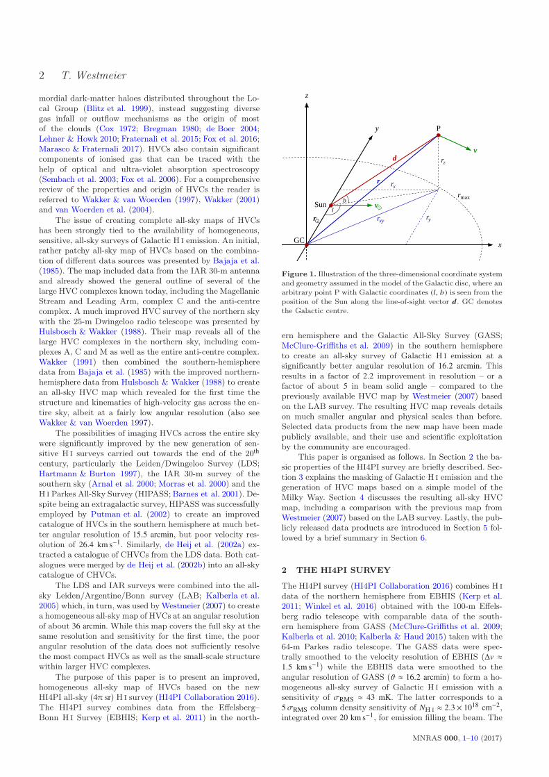
Figure 1. Illustration of the three-dimensional coordinate systemand geometry assumed in the model of the Galactic disc, where anarbitrary point P with Galactic coordinates (l, b) is seen from theposition of the Sun along the line-of-sight vector d. GC denotesthe Galactic centre.

ern hemisphere and the Galactic All-Sky Survey (GASS;McClure-Griffiths et al. 2009) in the southern hemisphereto create an all-sky survey of Galactic H I emission at asignificantly better angular resolution of 16.2 arcmin. Thisresults in a factor of 2.2 improvement in resolution – or afactor of about 5 in beam solid angle – compared to thepreviously available HVC map by Westmeier (2007) basedon the LAB survey. The resulting HVC map reveals detailson much smaller angular and physical scales than before.Selected data products from the new map have been madepublicly available, and their use and scientific exploitationby the community are encouraged.

This paper is organised as follows. In Section 2 the ba-sic properties of the HI4PI survey are briefly described. Sec-tion 3 explains the masking of Galactic H I emission and thegeneration of HVC maps based on a simple model of theMilky Way. Section 4 discusses the resulting all-sky HVCmap, including a comparison with the previous map fromWestmeier (2007) based on the LAB survey. Lastly, the pub-licly released data products are introduced in Section 5 fol-lowed by a brief summary in Section 6.

2 THE HI4PI SURVEY

The HI4PI survey (HI4PI Collaboration 2016) combines H I

data of the northern hemisphere from EBHIS (Kerp et al.2011; Winkel et al. 2016) obtained with the 100-m Effels-berg radio telescope with comparable data of the south-ern hemisphere from GASS (McClure-Griffiths et al. 2009;Kalberla et al. 2010; Kalberla & Haud 2015) taken with the64-m Parkes radio telescope. The GASS data were spec-trally smoothed to the velocity resolution of EBHIS (∆v ≈1.5 km s−1) while the EBHIS data were smoothed to theangular resolution of GASS (ϑ ≈ 16.2 arcmin) to form a ho-mogeneous all-sky survey of Galactic H I emission with asensitivity of σRMS ≈ 43 mK. The latter corresponds to a5σRMS column density sensitivity of NH I ≈ 2.3 × 1018 cm−2,integrated over 20 km s−1, for emission filling the beam. The

MNRAS 000, 1–10 (2017)

All-sky map of high-velocity clouds 3

LSR velocity coverage is about ±480 km s−1 in the southernhemisphere and ±600 km s−1 in the northern hemisphere.The HVC map presented here is restricted to the narrowervelocity coverage of the GASS data to ensure a homogeneouscoverage across the sky. As virtually all HVC emission is re-stricted to velocities of |vLSR | < 450 km s−1, the chosen veloc-ity cut-off is not expected to have any effect on the qualityand completeness of the HVC map.

3 DATA PROCESSING

3.1 Model of the Galactic H I disc

Creation of an all-sky HVC map requires masking of H I

emission from the Galactic disc. Hence, the first step willbe to develop a three-dimensional model of the Milky Way’sneutral gas disc. For the sake of simplicity, a simple cylin-drical geometry of the Galactic disc is assumed, similar tothe approach by Wakker (1991) who concluded that the pu-rity of the resulting HVC map is not particularly sensitiveto the details of the model. The basic Galactocentric coor-dinate system used here is illustrated in Fig. 1, where thex and y axes define the Galactic plane, while the z axis isperpendicular to the plane and pointing in the direction ofthe north Galactic pole. The Sun is assumed to be located inthe Galactic plane at the position of r⊙ = (0,r⊙ ,0) and mov-ing in positive x-direction at a velocity of v⊙ = (v⊙ ,0,0).1

Throughout this paper the standard values of r⊙ = 8.5 kpc

and v⊙ = 220 km s−1 adopted by the International Astro-nomical Union (Kerr & Lynden-Bell 1986) are assumed.

Let us further introduce a point P with radius vectorr = (rx ,ry ,rz ) at which the gas is moving at a velocity ofv = (vx ,vy ,0). Following the geometry in Fig. 1, the positionof P is given as

r =*.,rxryrz

+/- =*.,

d sin(l) cos(b)

r⊙ − d cos(l) cos(b)

d sin(b)

+/- (1)

where l and b are the Galactic longitude and latitude, respec-tively, of the line-of-sight vector, d, pointing from the Sun topoint P. Next, we need to determine the radial velocity of thegas at P relative to the Sun by projecting the velocity vec-tor, v, on to the line-of-sight vector, d, and subtracting theprojected contribution from the Sun’s own orbital velocity,thus

vrad =d · (v − v⊙ )

|d |=

(r − r⊙ ) · (v − v⊙ )

d. (2)

Inserting Eq. 1 into Eq. 2, we obtain the following expressionfor the radial velocity:

vrad =

[vrot(rxy )

r⊙

rxy− v⊙

]sin(l) cos(b) (3)

where vrot (rxy ) is the rotation curve of the Milky Way andrxy = |(rx ,ry ) |. Note that the geometry used here impliescylindrical rotation, i.e. the rotation velocity of the disc isassumed to be independent of height, z, above the Galacticplane.

1 Strictly speaking, this velocity refers to the LSR, as the Sunpossesses a small peculiar motion with respect to the LSR.

For this work, the rotation curve of Clemens (1985) isused, specifically the polynomial fit to the rotation curve forthe IAU standard values of r⊙ = 8.5 kpc and v⊙ = 220 km s−1.The rotation curve of Clemens (1985) was derived from com-bined CO and H I observations of the Milky Way and shouldtherefore be well-suited to describe the rotation velocity ofthe neutral gas disc for the purpose of identifying high-velocity emission.

With the radial velocity of any arbitrary point at hand,we can now determine the velocity range of Galactic discgas for any position in the sky by simply moving away fromthe Sun in discrete steps along the line of sight, determiningthe radial velocity of the gas in each step, and recording themaximum and minimum values, vmax and vmin, encounteredin between the Sun and the boundary of the cylindrical discmodel. Lastly, the derived velocity range will need to beexpanded by a fixed deviation velocity, vdev, to account forthe intrinsic velocity dispersion of the disc gas as well as anysmall deviations from the regular rotation velocity of the disc(Wakker 1991). The final velocity range, [vmin − vdev,vmax +

vdev], can then be masked in the data cube, leaving onlychannels with velocities inconsistent with Galactic rotation.

3.2 Optimisation of model parameters

While we now have a simple model of the Galactic disc thatwill allow us to mask and remove Galactic H I emission, thereare several free parameters, specifically the disc size, rmax

and zmax, as well as the value of the deviation velocity, vdev,that will need to be chosen first. For this purpose, a low-resolution copy of the entire HI4PI survey was created bybinning the data by a factor of 8 in the spatial domain and 4in the spectral domain. This reduced the total data volumeby a factor of 256, allowing for fast processing of the full skyat low resolution.

Next, maps of HVC emission were calculated from thebinned data using a matrix of different values for the threefree parameters. The following set of parameter values weretested in this way: rmax = 20, 25 and 30 kpc, zmax = 2, 5

and 10 kpc, and vdev = 50, 60 and 70 km s−1. This resultedin a total of 27 different parameter combinations to be pro-cessed and tested. The HVC maps resulting from the dif-ferent combinations of parameters were finally inspected byeye to determine the parameter values that would success-fully remove most of the Galactic foreground H I emissionwhile retaining as much of the H I emission from the HVCpopulation as possible.

The resulting optimal set of disc parameters is rmax =

20 kpc, zmax = 5 kpc and vdev = 70 km s−1. Interestingly,varying the value of rmax did not have any significant influ-ence on the result, while changing the thickness of the discled to substantial changes in the purity of the resulting HVCmap. Similarly, choosing a lower deviation velocity would in-troduce significant residuals from intermediate-velocity gas,e.g. in the region of complex M. Compared to the parame-ters adopted by Wakker (1991), the disc radius chosen hereis smaller, while the thickness of the disc and deviation ve-locity are larger. This results in a ‘cleaner’ map with lowerlevels of residual emission from the Galactic disc (e.g. in theregion of the Outer Arm), while the major HVC complexesare largely unaffected due to their significant kinematic sep-aration from the disc.

MNRAS 000, 1–10 (2017)

4 T. Westmeier

LSRv km s( −1)

1020

IH

N(c

m−

2)

−90°

−60°

−30°

Gal

actic

latit

ude

0°

30°

60°

90°

360° 300°

II I

IIIIV

VIV

IVIII

II

0

III I

CD Ce

Ce

V

IV

III

Stream

Cohen

Giovanelli Stream

III

II

I

Region

Interface

IV

I

II IIIAnti−

Shell

K

K

GCN

AC

AC

MSMS

LA

WE

LA

LA

M33

M31

LMC

SMC

WB/WA

B

A

H

C

4802400−240−480

0°

Galactic longitude

240° 60°120°

C

180°

I II

0

I

Bridge

Centre

MagellanicWright’sCloud

M

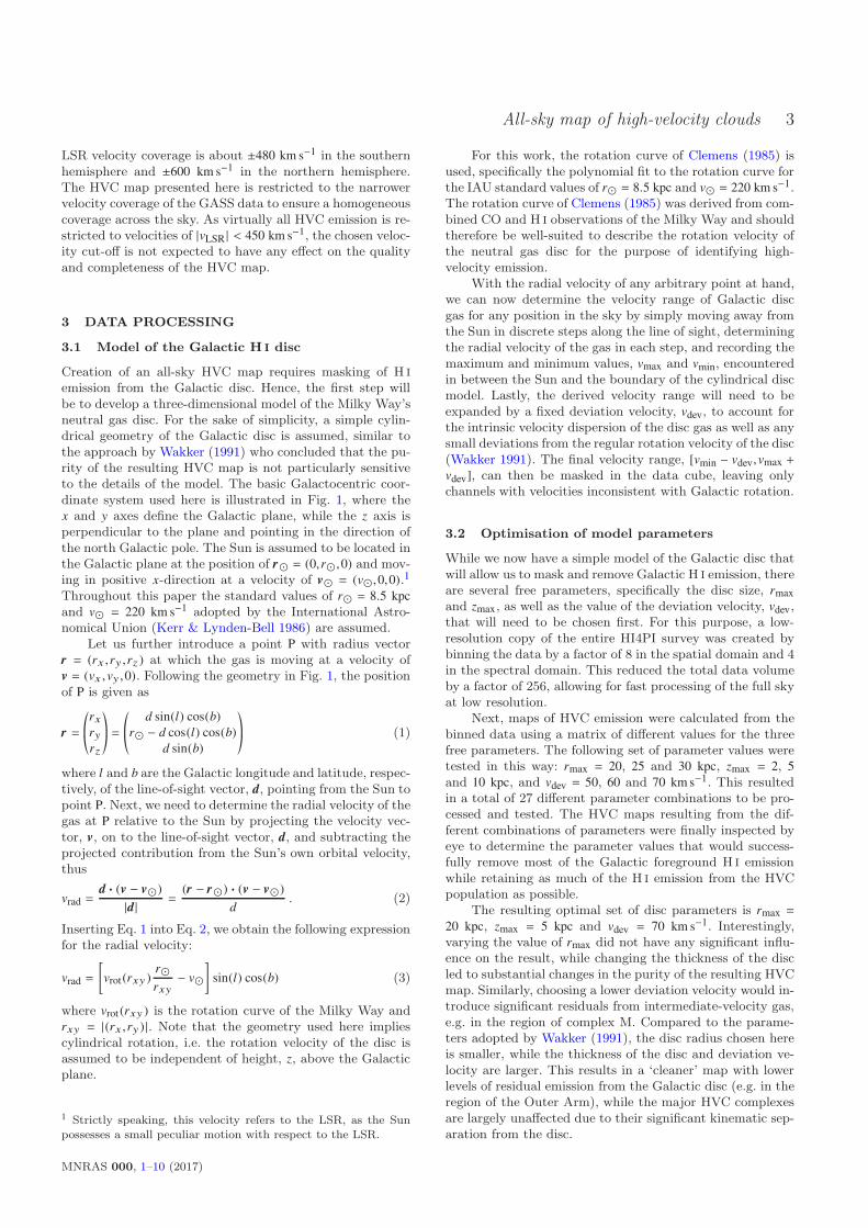
Figure 2. All-sky false-colour map of high-velocity gas presented in Hammer–Aitoff projection in Galactic coordinates centred on theGalactic anti-centre. Brightness and hue in the image represent H I column density (linear from 0 to 1020 cm−2) and LSR radial velocity ofthe emission, respectively. Several major HVC complexes as well as a few notable individual structures and external galaxies are labelled.

3.3 Generation of HVC maps

After determination of the optimal set of parameters for theGalactic disc model, a custom script written in C++ wasused to process the original HI4PI data with the aim ofgenerating an all-sky map of HVCs. The script first readsan HI4PI sub-cube of 20 × 20 into memory. It then loopsacross all spatial pixels of the cube, extracts the Galacticcoordinates at each pixel, and applies Eq. 3 to determinethe velocity range of Galactic emission at that position bymoving outwards from the Sun along the line of sight insteps of 100 pc. All spectral channels located within thatGalactic velocity range, expanded by the deviation velocityof 70 km s−1, are then masked before the processed cube iswritten back to disk for subsequent analysis.

In order to facilitate the creation of two-dimensionalmaps of the HVC sky from the masked data cubes, themasked cubes were first smoothed spatially by a Gaussian of48 arcmin FWHM and spectrally by a boxcar filter 5 channels(approximately 7.5 km s−1) wide. Only those pixels of theoriginal cube that had TB > 50 mK in the smoothed copy ofthe cube were used in the generation of any two-dimensionalmaps created from the data cube. This approach ensuresthat the faint outer parts of diffuse H I sources are includedin the map, while compact artefacts such as noise and radiofrequency interference (RFI) are largely excluded. Lastly,any two-dimensional HVC maps created from the maskeddata cubes were concatenated to form a single, all-sky map.

The resulting two-dimensional all-sky HVC map inHammer–Aitoff projection is presented in Fig. 2 in Galac-tic coordinates centred on the Galactic anti-centre. In thiscolour map, which was created to facilitate visual inspec-tion of the HVC emission, brightness represents H I column

density, while hue reflects the LSR radial velocity of theemission. This allows HVCs of different velocities to be dis-tinguished by their different hues in regions of spatially over-lapping emission. The naming of HVC features in the mapis in accordance with Wakker (2001), Putman et al. (2003),Wakker (2004), Bruns et al. (2005), Venzmer et al. (2012)and For et al. (2013).

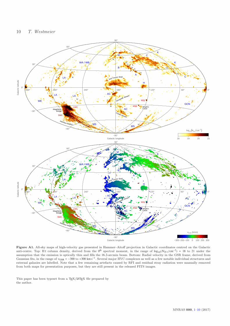
To provide data products that are more suitable for aquantitative analysis, a two-dimensional map of the 0th spec-tral moment was created as well. The 0th moment map wasconverted to H I column density in units of cm−2, using thestandard conversion factor of 1.823 × 1018 cm−2/(K km s−1),under the assumption that the emission is optically thin andfills the 16.2 arcmin beam. A labelled all-sky view of the re-sulting column density map in Hammer–Aitoff projectionin Galactic coordinates is presented in the upper panel ofFig. A1 in Appendix A.

In a similar fashion one could generate a radial velocitymap of the HVC sky from the 1st spectral moment. However,a general issue with the 1st moment is that the resulting val-ues may be highly susceptible to the influence of noise incases where either the H I signal is faint or the applied maskis too large. In addition, the 1st moment may produce arbi-trary values in cases where multiple sources of emission existalong the line of sight. In order to avoid these issues, a veloc-ity map was created by fitting a single Gaussian function tothe brightest line component in each spectrum using a cus-tom script written in python. The script will first identifythe location of the brightest emission in the spectrum, thendetermine the mean and standard deviation of the emissionwithin a window of ±20 channels around that position, andfinally use those initial estimates to fit a Gaussian function

MNRAS 000, 1–10 (2017)

All-sky map of high-velocity clouds 5

HI4PI

Complex C

Complex B

AV

AIII

AII

A0

CIII

AI

Holmberg I

Holmberg II

NGC 2403

NGC 2366

M81

NGC 2841

IC 2574

NGC 2541

Complex A

AVI

AIV

LAB

Complex C

Complex B

AV

AIII

AII

A0

CIII

AINGC 2403

M81

Complex A

AVI

AIV

log 1

0(

HI

cm−

2N

)/

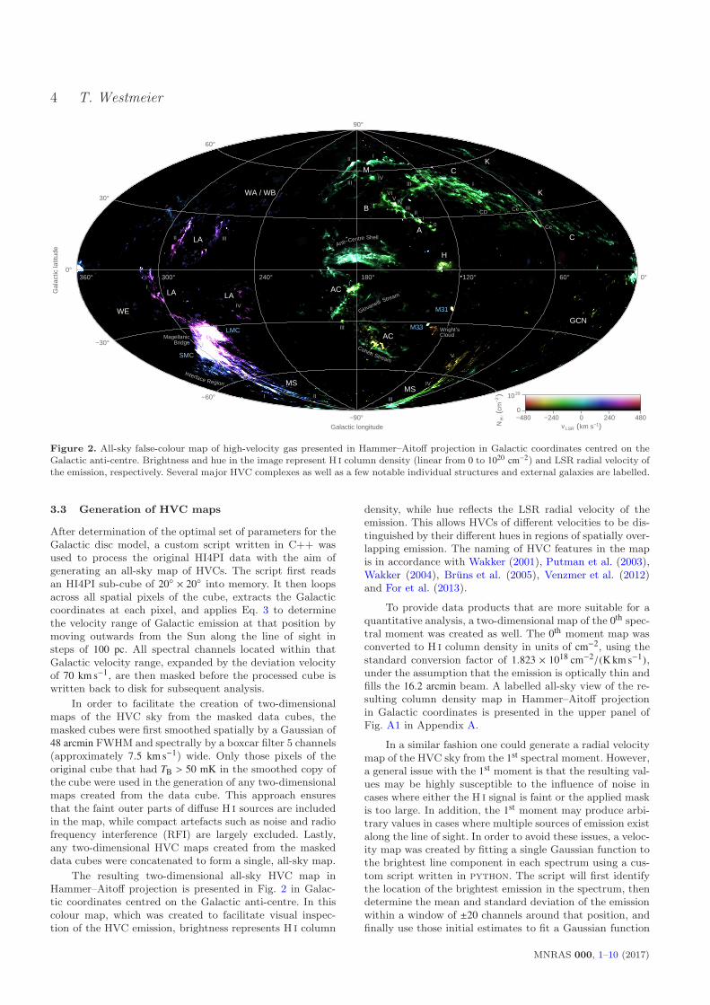
Figure 3. Comparison between the old HVC map from Westmeier (2007) based on LAB data (left) and the new map presented here

based on HI4PI data (right) in the region of HVC complex A. The substantial improvement in angular resolution reveals a complexnetwork of intricate gas filaments and clumps that are not resolved by the old LAB data. Note the large number of nearby galaxies visiblein the high-resolution HI4PI data, the brightest of which have been labelled.

to the entire spectrum. Successful fits are accepted for spec-tra that have positive integrated flux, a peak brightness tem-perature exceeding three times the mean RMS of the HI4PIsurvey (i.e. TB ≥ 130 mK), and an initial estimate of the stan-dard deviation of at least two channels (i.e. σ & 2.6 km s−1).The amplitude, mean and standard deviation from acceptedGaussian fits are then written into a FITS file for furtheranalysis.

As the native LSR velocity frame of the HI4PI data isdominated by the projected rotation velocity of the Galacticdisc, the resulting velocity map was converted to the moreappropriate Galactic standard-of-rest (GSR) frame in unitsof km s−1, assuming the standard orbital velocity of v⊙ =

220 km s−1 in the direction of (l,b) = (90,0). The resultingGSR velocity map of the HVC sky in Galactic coordinatesis presented in the bottom panel of Fig. A1 in Appendix A.

Finally, in order to facilitate studies of the Magellanicsystem, the H I column density and GSR velocity mapswere converted from the native Galactic coordinate system,(l,b), to Magellanic coordinates, (lMag,bMag), as defined byNidever et al. (2008). The resulting maps are presented inFig. A2 in Appendix A. The Magellanic coordinate system isdefined such that the Magellanic Stream and Leading Armare approximately aligned with the equator at bMag ≈ 0,while the Large Magellanic Cloud defines the origin of thelongitudinal axis at lMag = 0. This avoids the usually strongdistortions of parts of the Magellanic system in standardequatorial and Galactic coordinates and provides a morenatural coordinate system suitable for studies of the Mag-ellanic system. Note that the maps in Fig. A2 have beencentred on lMag = 270 instead of 0 to prevent Complex Cfrom being wrapped around the edge of the map.

4 RESULTS AND DISCUSSION

4.1 The HVC sky

The all-sky maps shown in Fig. 2 as well as Fig. A1 and A2show the major HVC complexes in the sky in much greater

detail than ever before. Dominant structures in the mapsinclude the large HVC complexes A, C and M in the north-ern (celestial and Galactic) hemisphere, the anti-centre com-plex and shell near the Galactic anti-centre, and the Magel-lanic Clouds with the extended structures of the MagellanicStream and Leading Arm mostly confined to the southernhemisphere. A few smaller or less sharply defined structuresare visible as well, including HVC complexes H and K. Sev-eral HVC complexes with low deviation velocities, most ofwhich kinematically overlap with Galactic disc emission, arelargely missing from the map, including complexes L, WA,WB, WC, G, R, GCP as well as parts of complex H and theGiovanelli Stream.

The final maps are almost entirely free of residual emis-sion from the Galactic disc. Notable contamination stemsfrom peculiar-velocity gas near the Galactic centre, faintintermediate-velocity gas filaments near the north Galac-tic pole, and a few remnants of extra-planar gas associatedwith the Outer Arm near (l,b) = (80 ,25). Moreover, not allemission seen in the maps is due to high-velocity H I gas. Onthe one hand, low levels of RFI and residual stray radiationmay still be present in some parts of the sky, in particular inthe northern celestial hemisphere covered by EBHIS. On theother hand, several nearby galaxies at low radial velocitiesare included in the map as well, most prominently the Largeand Small Magellanic Cloud as well as M31 and M33.

It should be noted that some of the HVC complexespartially extend into the velocity range of Galactic disc gas,which inevitably leads to the loss of some emission fromthe maps. As a consequence, the column density values insome regions of Fig. A1 and A2 may be lower limits whilethe velocities may be inaccurate. The Magellanic Streamin particular crosses from negative to positive LSR veloc-ities near the south Galactic pole, inevitably resulting influx loss. For the same reason, some neutral gas clouds lo-cated in the Galactic halo may be missing entirely, as theirkinematics in combination with the viewing geometry mayhave placed them within the deviation velocity range ap-plied here. This would effectively ‘hide’ those clouds within

MNRAS 000, 1–10 (2017)

6 T. Westmeier

Ori Dwarf

‘Hook’ ACI

AC Shell

Complex AC

ACIII

Giovanelli Stream

NGC 1156

ACII

HI4PILAB

‘Hook’ ACI

AC Shell

Complex AC

ACIII

Giovanelli Stream

ACII

cmI/

HN

−2 )

(10

log

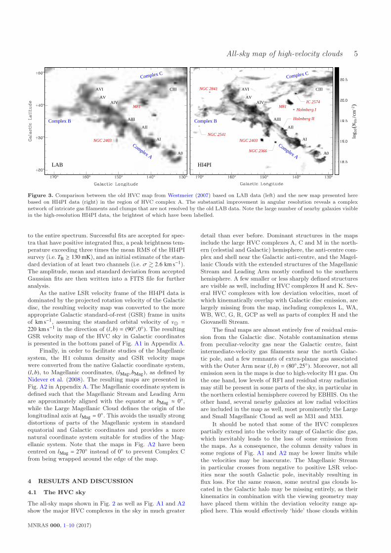
Figure 4. Same as in Fig. 3, but for a larger region around the northern section of the anti-centre (AC) complex and the adjacentanti-centre shell.

the velocity range of the Galactic disc, where they would nolonger be discernible as high-velocity gas.

4.2 Comparison with LAB data

Using the regions around HVC complex A and the anti-centre (AC) complex as an example, Fig. 3 and 4 comparethe quality of the previous all-sky map created by Westmeier(2007) based on LAB data with the new HI4PI-based mappresented here. While the individual clouds of complex Awere barely resolved by the 36 arcmin beam of the LABsurvey, the new data resolve complex A into a remarkablenetwork of intricate H I filaments and small clumps. Assum-ing a distance in the range of 4 to 10 kpc for complex A(van Woerden et al. 1999), the corresponding physical reso-lution would be in the range of about 20 to 50 pc. A similareffect can be seen in the anti-centre region, where the ACshell in particular breaks up into a system of fine, interwo-ven gas filaments that were too narrow to be resolved by the36 arcmin beam of the LAB survey in the past.

An additional improvement in the quality of the mapcan be attributed to the full spatial sampling of the HI4PIsurvey data in contrast to the LAB data which were onlysampled on a 30 arcmin grid. The undersampling of the LABsurvey is clearly visible in the left-hand panels of Fig. 3and 4. On top of the improvements in resolution and sam-pling, the HI4PI survey is also more sensitive than the LABsurvey, resulting in a better column density sensitivity2 ofabout 2.3×1018 cm−2 (as compared to about 3.7×1018 cm−2

for the LAB survey across a much larger beam solid angle).The significant improvement in both angular resolution andsensitivity is also highlighted by the large number of nearbygalaxies visible in the HI4PI map in the right-hand panel of

2 H I column density sensitivities are specified for a signal of 5 ×

σRMS across 20 km s−1 under the assumption that the emission isoptically thin and fills the beam size.

Fig. 3, only the brightest and most extended of which arealso seen in the LAB data.

Lastly, the general agreement between the LAB andHI4PI maps is remarkable in view of the fact that a slightlydifferent methodology was used byWestmeier (2007) for gen-erating the LAB-based HVC map. Nevertheless, the samegeneral features are visible in the two maps, indicating thatmost of the HVC structures in the sky are kinematicallywell-separated from the Galactic disc and thus appear inboth maps.

4.3 Sky coverage fraction of HVCs

From the resulting HVC map one can immediately derivethe sky coverage fraction of high-velocity H I emission as afunction of column density. For this purpose, column den-sity values were extracted from the map in plate carree pro-jection on a grid of ∆b = 0.25 deg in Galactic latitude and∆l cos(b) = 0.25 deg in Galactic longitude, resulting in a totalof about 4π/Ωgrid ≈ 660,000 largely independent data pointsacross the full sky. The resulting sky coverage fraction, fsky,and cumulative sky coverage fraction, φsky, of HVC emis-sion in excess of a given H I column density level are shownas the blue squares in Fig. 5. The cumulative sky coveragefraction for HVC emission of NH I > 2 × 1018 cm−2 is ap-proximately 15 per cent. It decreases to about 7 per cent atNH I > 1019 cm−2 and about 1 per cent at NH I > 1020 cm−2.

The original HVC map still contains some emissionfrom sources other than HVCs, in particular nearby galax-ies, residual emission from the Galactic disc and stray radi-ation residuals in the northern celestial hemisphere coveredby EBHIS. Therefore, a cleaned HVC map was created bymanually masking bright galaxies (including the LMC, SMCand Magellanic Bridge, but not the Interface Region, Mag-ellanic Stream and Leading Arm), bright emission near theGalactic centre, residual emission from the Outer Arm andbright stray radiation residuals in the EBHIS data. The mea-surements of fsky and φsky resulting from the cleaned map

MNRAS 000, 1–10 (2017)

All-sky map of high-velocity clouds 7

18.0 18.5 19.0 19.5 20.0 20.5 21.0 21.5 22.0−6

−5

−4

−3

−2

−1

0

Fit

Data raw

Data clean

LAB

0

−2

−4

−1

−3

−5

−618 19 20 21 22

log

10(f

sky)

N cm/HI−2log10 )(

10%

1%

Schechter function fitLAB dataHI4PI data cleanedHI4PI data original

Sky coverage

18.0 18.5 19.0 19.5 20.0 20.5 21.0 21.5 22.0−6

−5

−4

−3

−2

−1

0

Data raw

Data clean

LAB

0

−2

−4

−1

−3

−5

−618 19 20 21 22

log

10sk

y)

(φ

N cm/HI−2

10 )(log

10%

1%

LAB dataHI4PI data cleanedHI4PI data original

Cumulative sky coverage

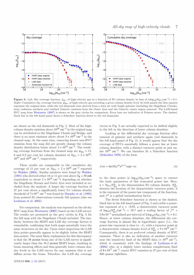
Figure 5. Left: Sky coverage fraction, fsky, of high-velocity gas as a function of H I column density in bins of ∆ log10 (NH I/cm−2) = 0.1.Right: Cumulative sky coverage fraction, φsky, of high-velocity gas exceeding a given column density level. In both panels the blue squaresrepresent the original data, while the red diamonds were derived from a data set with bright galaxies (including the Magellanic Clouds),stray radiation artefacts and residual Galactic emission from the Outer Arm and the Galactic centre region removed. The LAB-basedHVC map from Westmeier (2007) is shown as the grey circles for comparison. Error bars are indicative of Poisson errors. The dashed,black line in the left-hand panel shows a Schechter function fitted to the red diamonds.

are shown as the red diamonds in Fig. 5. Most of the high-column density emission above 1020 cm−2 in the original mapcan be attributed to the Magellanic Clouds and Bridge, andthere is no more emission above about 5 × 1020 cm−2 in thecleaned map. At the same time, removing known non-HVCemission from the map did not greatly change the columndensity distribution below about 3 × 1019 cm−2. The result-ing coverage fractions from the cleaned map are φsky ≈ 13,

6 and 0.2 per cent for column densities of NH I > 2 × 1018,1019 and 1020 cm−2, respectively.

These results are comparable to the cumulative skycoverage of 15 per cent at NH I > 2 × 1018 cm−2 reportedby Wakker (2004). Similar numbers were found by Wakker(1991) who derived either 18 or 11 per cent above TB = 50 mK

(equivalent to about 2 × 1018 cm−2) depending on whetherthe Magellanic Stream and Outer Arm were included or ex-cluded from the analysis. A larger sky coverage fraction of37 per cent above a significantly lower 5σ column densitythreshold of 7×1017 cm−2 was found by Murphy et al. (1995)from pointed H I observations towards 102 quasars (also seeLockman et al. 2002).

For comparison, the analysis was repeated on the all-skyHVC map from Westmeier (2007) based on the LAB survey.The results are presented as the grey circles in Fig. 5 forthe full map with the Magellanic Clouds included. The sim-ilarity between the HI4PI and LAB sky coverage factors isremarkable, confirming that both maps essentially trace thesame structures on the sky. Upon closer inspection the LABdata points generally appear to be slightly below the HI4PIdata points. The most likely explanation for this discrepancyis that the 36 arcmin beam size of the LAB survey is signifi-cantly larger than the 16.2 arcmin HI4PI beam, resulting inbeam smearing effects and thus generally lower column den-sity levels in the LAB survey for any emission that is notdiffuse across the beam. Therefore, the LAB sky coverage

curves in Fig. 5 are actually expected to be shifted slightlyto the left in the direction of lower column densities.

Looking at the differential sky coverage fraction afterremoval of galaxies and artefacts again (red diamonds inthe left-hand panel of Fig. 5), it would appear that the skycoverage of HVCs essentially follows a power law at lowercolumn densities, with a distinct turnover point at just un-der 1020 cm−2. We can therefore fit a Schechter function(Schechter 1976) of the form

f (n) = ln(10) f ⋆nα+1 exp(−n) (4)

to the data points in log10 (NH I/cm−2) space to extractthe basic parameters of this truncated power law. Here,n = NH I/N

⋆H I

is the dimensionless H I column density, N⋆H I

denotes the location of the characteristic turnover point, αis the exponent of the power-law component of the function,and f ⋆ is a global normalisation factor.

The fitted Schechter function is shown as the dashed,black line in the left-hand panel of Fig. 5 and yields a power-law exponent of α = −0.93, a characteristic turnover pointof log10 (N⋆

H I/cm−2) = 19.7 and a scaling factor of f ⋆ =

5.0×10−3 normalised per interval of ∆ log10 (NH I/cm−2) = 0.1.Hence, at lower column densities, the differential sky cov-erage fraction is almost flat in logarithmic space (i.e., thepower-law exponent is close to −1), with a turnover point ata characteristic column density level of N⋆

H I≈ 5×1019 cm−2.

Consequently, there is no preferred column density of HVCemission. There is also no indication of another turnovernear the sensitivity limit of the HI4PI data (≈ 1018 cm−2),which is consistent with the findings of Lockman et al.(2002) who, at a slightly lower median completeness limitof 8×1017 cm−2, report HVC emission in 37 per cent of their860 quasar sightlines.

MNRAS 000, 1–10 (2017)

8 T. Westmeier

Table 1. List of FITS data products made available as supplementary material in the online version of this paper. The standard FITSprojection codes used are CAR (plate carree) and AIT (Hammer–Aitoff). File sizes are given for the compressed files in units of 1 MB = 220 B.

Data product Coordinate Proj. Dimension File name File size

system (pixels) (MB)

log10 (NH I/cm−2) Galactic CAR 4323 × 2144 hi4pi-hvc-nhi-gal-car.fits.gz 7.7

log10 (NH I/cm−2) Galactic AIT 3891 × 1947 hi4pi-hvc-nhi-gal-ait.fits.gz 4.6

log10 (NH I/cm−2) Magellanic CAR 4323 × 2144 hi4pi-hvc-nhi-mag-car.fits.gz 7.9

vLSR/(km s−1) Galactic CAR 4323 × 2144 hi4pi-hvc-vlsr-gal-car.fits.gz 4.5

vLSR/(km s−1) Galactic AIT 3891 × 1947 hi4pi-hvc-vlsr-gal-ait.fits.gz 2.9

vGSR/(km s−1) Galactic CAR 4323 × 2144 hi4pi-hvc-vgsr-gal-car.fits.gz 4.6

vGSR/(km s−1) Galactic AIT 3891 × 1947 hi4pi-hvc-vgsr-gal-ait.fits.gz 3.0

vGSR/(km s−1) Magellanic CAR 4323 × 2144 hi4pi-hvc-vgsr-mag-car.fits.gz 4.7

5 DATA RELEASE

All-sky HVC maps are a useful tool for a wide rangeof scientific applications, including, among others, thestudy of the HVC population itself (Wakker 1991;Wakker & van Woerden 1991), comparison of the H I emis-sion with optical and ultra-violet absorption lines of ionisedgas in the Galactic halo (Fox et al. 2006; Lehner et al.2012), cross-correlation of the H I emission with X-rayemission (Kerp et al. 1996, 1999; Shelton et al. 2012) andHα emission (Tufte et al. 1998; Barger et al. 2012), andcomparison of the H I gas with molecular gas (Wakker et al.1997) and dust emission (Wakker & Boulanger 1986;Miville-Deschenes et al. 2005; Williams et al. 2012;Lenz et al. 2016) in the quest for evidence of star for-mation in HVC complexes such as the Magellanic Stream(Tanaka & Hamajima 1982; Bruck & Hawkins 1983) andLeading Arm (Casetti-Dinescu et al. 2014).

In order to facilitate a wider scientific use of the newall-sky HVC maps by the community, H I column densitymaps and radial velocity maps in the LSR and GSR frameshave been made publicly available in both plate carree andHammer–Aitoff projections (see Table 1 for details). Themaps are provided as two-dimensional FITS images (Flex-ible Image Transport System; Wells et al. 1981) and areavailable as supplementary material in the online versionof this paper. Column density and GSR velocity maps inplate carree projection are also made available in Magel-lanic coordinates (using the definition of Nidever et al. 2008)in which the Magellanic Stream is aligned with the equa-tor to facilitate studies of the Magellanic system. Note thatfor convenience the corresponding FITS files have Galacticcoordinates defined in their header, as the FITS standarddoes not natively support the Magellanic coordinate system(Calabretta & Greisen 2002), while user-specific coordinatesystems may not be supported by some of the third-partysoftware commonly used to handle and display FITS images.

6 SUMMARY

In this paper a new all-sky map of Galactic HVCs basedon the HI4PI survey is presented. For this purpose, a sim-ple, cylindrical model of the Galactic disc with a disc radiusof 20 kpc and a disc height of 5 kpc was created based onwhich the expected velocity range of Galactic emission wasdetermined and masked after applying an additional devi-

ation velocity of 70 km s−1. All-sky H I column density andvelocity maps of high-velocity gas were then generated fromthe masked cubes.

The resulting all-sky maps show the Milky Way’sHVC population at an unprecedented angular resolution of16.2 arcmin and a 5σ column density sensitivity of about2.3×1018 cm−2. Most of the HVC complexes are resolved intoa network of H I filaments and clumps not seen in the pre-vious HVC maps of Wakker (1991) and Westmeier (2007).The overall sky coverage fraction of high-velocity gas is ap-proximately 15 per cent for emission of NH I > 2×1018 cm−2,decreasing to about 13 per cent when the Magellanic Cloudsand some additional non-HVC emission are excluded. Thedifferential HVC sky coverage fraction as a function of col-umn density essentially follows a truncated power law withan exponent of −0.93 and a characteristic turnover point ata column density level of about 5 × 1019 cm−2.

FITS files of H I column density and velocity maps ofthe HVC sky in different coordinate systems and projectionshave been made publicly available to facilitate the scientificuse of the new HVC map by the entire community. Usersare requested to include a reference to this paper in anypublication making use of these data files.

ACKNOWLEDGEMENTS

The author would like to thank L. Staveley-Smith for valu-able discussions and comments on the manuscript. This workis based on publicly released data from the HI4PI surveywhich combines the Effelsberg–Bonn H I Survey (EBHIS)in the northern hemisphere with the Galactic All-Sky Sur-vey (GASS) in the southern hemisphere. This publicationis based on observations with the 100-m telescope of theMPIfR (Max-Planck-Institut fur Radioastronomie) at Ef-felsberg. The Parkes Radio Telescope is part of the Aus-tralia Telescope which is funded by the Commonwealth ofAustralia for operation as a National Facility managed byCSIRO. This research has made use of the VizieR catalogueaccess tool, CDS, Strasbourg, France. The original descrip-tion of the VizieR service was published in A&AS 143, 23.This research has made use of NASA’s Astrophysics DataSystem Bibliographic Services. This research has made useof the NASA/IPAC Extragalactic Database (NED), which isoperated by the Jet Propulsion Laboratory, California Insti-tute of Technology, under contract with the National Aero-nautics and Space Administration.

MNRAS 000, 1–10 (2017)

All-sky map of high-velocity clouds 9

REFERENCES

Adams E. A. K., Giovanelli R., Haynes M. P., 2013, ApJ, 768, 77

Arnal E. M., Bajaja E., Larrarte J. J., Morras R., PoppelW. G. L., 2000, A&AS, 142, 35

Bajaja E., Cappa de Nicolau C. E., Cersosimo J. C., Martin M. C.,Loiseau N., Morras R., Olano C. A., Poppel W. G. L., 1985,ApJS, 58, 143

Barger K. A., Haffner L. M., Wakker B. P., Hill A. S., MadsenG. J., Duncan A. K., 2012, ApJ, 761, 145

Barnes D. G., et al., 2001, MNRAS, 322, 486

Blitz L., Spergel D. N., Teuben P. J., Hartmann D., Burton W. B.,1999, ApJ, 514, 818

Braun R., Burton W. B., 1999, A&A, 341, 437

Bregman J. N., 1980, ApJ, 236, 577

Bruck M. T., Hawkins M. R. S., 1983, A&A, 124, 216

Bruns C., et al., 2005, A&A, 432, 45

Calabretta M. R., Greisen E. W., 2002, A&A, 395, 1077

Casetti-Dinescu D. I., Moni Bidin C., Girard T. M., Mendez R. A.,Vieira K., Korchagin V. I., van Altena W. F., 2014, ApJ, 784,L37

Clemens D. P., 1985, ApJ, 295, 422

Cox D. P., 1972, ApJ, 178, 159

Danly L., Albert C. E., Kuntz K. D., 1993, ApJ, 416, L29

For B.-Q., Staveley-Smith L., McClure-Griffiths N. M., 2013, ApJ,764, 74

Fox A. J., Savage B. D., Wakker B. P., 2006, ApJS, 165, 229

Fox A. J., et al., 2016, ApJ, 816, L11

Fraternali F., Marasco A., Armillotta L., Marinacci F., 2015, MN-RAS, 447, L70

HI4PI Collaboration 2016, A&A, 594, A116

Hartmann D., Burton W. B., 1997, Atlas of Galactic NeutralHydrogen. Cambridge University Press

Hulsbosch A. N. M., 1968, Bull. Astron. Inst. Netherlands, 20, 33

Hulsbosch A. N. M., Wakker B. P., 1988, A&AS, 75, 191

Kalberla P. M. W., Haud U., 2015, A&A, 578, A78

Kalberla P. M. W., Burton W. B., Hartmann D., Arnal E. M.,Bajaja E., Morras R., Poppel W. G. L., 2005, A&A, 440, 775

Kalberla P. M. W., et al., 2010, A&A, 521, A17

Kerp J., Mack K.-H., Egger R., Pietz J., Zimmer F., Mebold U.,Burton W. B., Hartmann D., 1996, A&A, 312, 67

Kerp J., Burton W. B., Egger R., Freyberg M. J., Hartmann D.,Kalberla P. M. W., Mebold U., Pietz J., 1999, A&A, 342, 213

Kerp J., Winkel B., Ben Bekhti N., Floer L., Kalberla P. M. W.,2011, Astron. Nachr., 332, 637

Kerr F. J., Lynden-Bell D., 1986, MNRAS, 221, 1023

Lehner N., Howk J. C., 2010, ApJ, 709, L138

Lehner N., Howk J. C., Thom C., Fox A. J., Tumlinson J., TrippT. M., Meiring J. D., 2012, MNRAS, 424, 2896

Lenz D., Floer L., Kerp J., 2016, A&A, 586, A121

Lockman F. J., Murphy E. M., Petty-Powell S., Urick V. J., 2002,ApJS, 140, 331

Marasco A., Fraternali F., 2017, MNRAS, 464, L100

Mathewson D. S., Cleary M. N., Murray J. D., 1974, ApJ, 190,291

McClure-Griffiths N. M., et al., 2009, ApJS, 181, 398

Miville-Deschenes M.-A., Boulanger F., Reach W. T., Noriega-Crespo A., 2005, ApJ, 631, L57

Morras R., Bajaja E., Arnal E. M., Poppel W. G. L., 2000, A&AS,142, 25

Muller C. A., Oort J. H., Raimond E., 1963, C. R. Acad. Sci.,257, 1661

Murphy E. M., Lockman F. J., Savage B. D., 1995, ApJ, 447, 642

Nidever D. L., Majewski S. R., Burton W. B., 2008, ApJ, 679,432

Oort J. H., 1966, Bull. Astron. Inst. Netherlands, 18, 421

Peek J. E. G., Bordoloi R., Sana H., Roman-Duval J., TumlinsonJ., Zheng Y., 2016, ApJ, 828, L20

Putman M. E., et al., 2002, AJ, 123, 873

Putman M. E., Staveley-Smith L., Freeman K. C., Gibson B. K.,Barnes D. G., 2003, ApJ, 586, 170

Savage B. D., de Boer K. S., 1981, ApJ, 243, 460Schechter P., 1976, ApJ, 203, 297Sembach K. R., et al., 2003, ApJS, 146, 165Shelton R. L., Kwak K., Henley D. B., 2012, ApJ, 751, 120Tanaka K. I., Hamajima K., 1982, PASJ, 34, 417Thom C., Peek J. E. G., Putman M. E., Heiles C., Peek K. M. G.,

Wilhelm R., 2008, ApJ, 684, 364Tufte S. L., Reynolds R. J., Haffner L. M., 1998, ApJ, 504, 773Venzmer M. S., Kerp J., Kalberla P. M. W., 2012, A&A, 547, A12Wakker B. P., 1991, A&A, 250, 499Wakker B. P., 2001, ApJS, 136, 463Wakker B. P., 2004, HVC/IVCMaps and HVC Distribution Func-

tions. Kluwer Academic Publishers, pp 25–54

Wakker B. P., Boulanger F., 1986, A&A, 170, 84Wakker B. P., van Woerden H., 1991, A&A, 250, 509Wakker B. P., van Woerden H., 1997, ARA&A, 35, 217Wakker B., Howk C., Schwarz U., van Woerden H., Beers T.,

Wilhelm R., Kalberla P., Danly L., 1996, ApJ, 473, 834Wakker B. P., Murphy E. M., van Woerden H., Dame T. M., 1997,

ApJ, 488, 216Wakker B. P., et al., 2007, ApJ, 670, L113Wakker B. P., York D. G., Wilhelm R., Barentine J. C., Richter

P., Beers T. C., Ivezic Z., Howk J. C., 2008, ApJ, 672, 298Wells D. C., Greisen E. W., Harten R. H., 1981, A&AS, 44, 363Westmeier T., 2007, PhD thesis, Rheinische Friedrich-Wilhelms-

Universitat BonnWilliams R. J., Mathur S., Poindexter S., Elvis M., Nicastro F.,

2012, AJ, 143, 82Winkel B., Kerp J., Floer L., Kalberla P. M. W., Ben Bekhti N.,

Keller R., Lenz D., 2016, A&A, 585, A41

de Boer K. S., 2004, A&A, 419, 527de Heij V., Braun R., Burton W. B., 2002a, A&A, 391, 159de Heij V., Braun R., Burton W. B., 2002b, A&A, 392, 417van Woerden H., Schwarz U. J., Peletier R. F., Wakker B. P.,

Kalberla P. M. W., 1999, Nature, 400, 138van Woerden H., Wakker B. P., Schwarz U. J., de Boer K. S., eds,

2004, High Velocity Clouds. Astrophysics and Space ScienceLibrary Vol. 312, Kluver Academic Publishers

SUPPORTING INFORMATION

Additional Supporting Information may be found in the on-line version of this paper:

As detailed in Section 5, FITS images of the new all-skymap of HVCs presented in this paper are made available assupplementary material in the online version of this paper.An overview of the individual data products and correspond-ing FITS files is provided in Table 1.

Please note: Oxford University Press are not responsiblefor the content or functionality of any supporting materialssupplied by the authors. Any queries (other than missingmaterial) should be directed to the corresponding authorfor the paper.

APPENDIX A: COLUMN DENSITY AND

VELOCITY MAPS

H I column density and GSR radial velocity maps of thehigh-velocity sky in Hammer–Aitoff projection in bothGalactic and Magellanic coordinates are presented in thisappendix.

MNRAS 000, 1–10 (2017)

10 T. Westmeier

log (N cm )10 HI−2/

LMC

−90°

−60°

−30°

Gal

actic

latit

ude

0°

30°

60°

90°

0°

LA

B

II I

IVIII

II

I

Anti−Shell

III

IV

M33

C

H

A

LA

MSMS

K

K

Cohen

III

Galactic longitude

III

VIV

0

II

III

LAIV

M31

Interface Region

VSMC

Ce

Ce

I

C

CD

IV

Giovanelli Stream

WEGCN

WB/WA

AC

AC

I

IIIII

Stream

60°300°360° 240° 180°

III

120°

18 19 20 21

Wright’sCloud

I

Centre

M

MagellanicBridge

vGSR (km/s)

−90°

−60°

−30°

Gal

actic

latit

ude

0°

30°

60°

90°

360° 0°

Anti−Shell

Cohen

Galactic longitude

Interface Region

Giovanelli Stream

MS

LALA

WE

LA

WB/WA

B

A

CK

K

C

GCN

AC

MS

AC

SMC

LMC M33

M31

Stream

300° 120° 60°240° 180°

H

Wright’sCloud

Centre

MagellanicBridge

100 3000−100 200−300−200

M

Figure A1. All-sky maps of high-velocity gas presented in Hammer–Aitoff projection in Galactic coordinates centred on the Galacticanti-centre. Top: H I column density, derived from the 0th spectral moment, in the range of log10(NH I/cm−2) = 18 to 21 under theassumption that the emission is optically thin and fills the 16.2-arcmin beam. Bottom: Radial velocity in the GSR frame, derived fromGaussian fits, in the range of vGSR = −300 to +300 km s−1. Several major HVC complexes as well as a few notable individual structures andexternal galaxies are labelled. Note that a few remaining artefacts caused by RFI and residual stray radiation were manually removedfrom both maps for presentation purposes, but they are still present in the released FITS images.

This paper has been typeset from a TEX/LATEX file prepared bythe author.

MNRAS 000, 1–10 (2017)

All-sky map of high-velocity clouds 11

log (N cm )10 HI−2/

−90°

−60°

−30°

Mag

ella

nic

latit

ude

0°

30°

60°

90°

Magellanic longitude

LA

LMCIII

III

I

IVII

II

Cohen Stream

C

IV

III

K

III

I

120°0° 300° 240° 180°60°

AC

VI

II

InterfaceRegion

LA

LA

III

B

A

H

WE

IV

SMC

MS

M31

M33I

VI

0

III

I

Ce

Ce

CD

C

90°90°

18 19 20 21

Anti−Centre Shell

M

Galactic Centre

WB/WA

Wright’sCloud

IV

vGSR )−1(km s

−90°

−60°

−30°

Mag

ella

nic

latit

ude

0°

30°

60°

90°

Magellanic longitude

LA

Cohen Stream

K

120°300° 240° 180°60°

InterfaceRegion

LA

LA

B

A

WE

M31

M33

C

90°90° 0°

SMC

LMCMS

AC

H

C

Anti−Centre Shell

M

Galactic Centre

WB/WA

Wright’sCloud

100 3000 200−100−300−200

Figure A2. Same as in Fig. A1, but using the Magellanic coordinate system as defined by Nidever et al. (2008). The coordinate systemis chosen such that the Magellanic Stream is aligned with the equator to facilitate studies of the Magellanic system. Note that the mapis centred on 270 in Magellanic longitude, as otherwise complex C would be wrapped around the edge of the map.

MNRAS 000, 1–10 (2017)