A NEW HEDONIC REGRESSION FOR REAL ESTATE PRICES APPLIED TO THE SINGAPORE RESIDENTIAL MARKET

By

Liang Jiang, Peter C. B. Phillips, and Jun Yu

December 2014

COWLES FOUNDATION DISCUSSION PAPER NO. 1969

COWLES FOUNDATION FOR RESEARCH IN ECONOMICS YALE UNIVERSITY

Box 208281 New Haven, Connecticut 06520-8281

http://cowles.econ.yale.edu/

A New Hedonic Regression for Real EstatePrices Applied to the Singapore

Residential Market∗

Liang JiangSingapore Management University

Peter C.B. PhillipsYale University, University of Auckland, University of Southampton,

Singapore Management University

Jun YuSingapore Management University

October 5, 2014

Abstract

This paper develops a new hedonic method for constructing a real estateprice index that utilizes all transaction price information that encompasses bothsingle-sale and repeat-sale properties. The new method is less prone to specifi-cation errors than standard hedonic methods and uses all available data. Likethe Case-Shiller repeat-sales method, the new method has the advantage of be-ing computationally effi cient. In an empirical analysis of the methodology, wefit the model to all transaction prices for private residential property holdings inSingapore between Q1 1995 and Q2 2014, covering several periods of major pricefluctuation and changes in government macroprudential policy. Two new indicesare created, one from all transaction prices and one from single-sales prices. Theindices are compared with the S&P/Case-Shiller index. The result shows that thenew indices slightly outperform the S&P/Case-Shiller index in predicting the priceof single-sales homes out-of-sample. However, they underperform the S&P/Case-Shiller index in predicting the price of repeat-sales homes out-of-sample. The

∗Jiang Liang, School of Economics, Singapore Management University, 90 Stamford Road, Sin-gapore. Peter C. B. Phillips, Yale University, 30 Hillhouse Avenue, New Haven, CT, 06520, USA;Email: peter.phillips@yale.edu; Phillips acknowledges research support from the NSF under GrantNo. SES 12-58258. Jun Yu, School of Economics and Lee Kong Chian School of Business, Sin-gapore Management University, 90 Stamford Road, Singapore. Email: yujun@smu.edu.sg. URL:http://www.mysmu.edu/faculty/yujun/. Yu thanks the Singapore Ministry of Education for Acad-emic Research Fund under grant number MOE2011-T2-2-096.

1

empirical findings indicate that specification bias can be more substantial thanthe sample selection bias when constructing a real estate price index. In a fur-ther empirical application, the recursive method of Phillips, Shi and Yu (2014)is used to detect explosive periods in real estate prices of Singapore. The resultsconfirm the existence of an explosive period from Q4 2006 to Q1 2008. No ex-plosive period is found after 2009, suggesting that the ten successive rounds ofcooling measures implemented by the Singapore government have been effectivein changing price dynamics and preventing a subsequent outbreak of explosivebehavior in the Singapore real estate market.

JEL classification: C58, R31Keywords: Repeat sales, Hedonic models, Prediction, Index, Explosive, Coolingmeasures

1 Introduction

Real estate prices are one of the key indicators of economic activity. Indices measuring

changes in real estate prices help to inform households about their asset wealth and

to make a wide variety of economic decisions that depend on wealth resources. Policy

makers rely on the information imported by these indices in designing and formulating

monetary and fiscal policies at the aggregate level as well as macro-prudential policies

directed at the financial and banking sectors. Though real estate prices are widely

accepted as highly important economic statistics, the construction of a suitable index

that will reflect movements in the price of a typical house in the economy presents many

conceptual, practical, and theoretical challenges.

First, houses are distinctive, making it particularly diffi cult to characterize a ‘typi-

cal’house for the development of an index. Different houses have varying characteristics

such as location, size, ownership, utilities and indoor/outdoor facilities. These differ-

ences imply that averaging all market transaction prices without controlling for house

heterogeneity inevitably produces bias. Second, house transactions are infrequent and

sales data are unbalanced for several reasons. Most houses on the market are single-

sale houses. Houses that have been sold more than once account for a small portion

of the whole market in a typical dataset. Also, houses sold in one period can be quite

different from those sold in other periods. These factors unbalance the pricing data and

complicate econometric construction of a price index due to problems of heterogeneous,

missing, and unequally spaced observations. Third, a typical presumption underlying

construction of real estate price indices is that the average quality of properties in the

market remains constant over time, whereas quality improvements in housing occurs

2

continuously from advances in materials, design, utilities, and construction technologies.

Meanwhile and in spite of ongoing maintenance, older dwellings age with the holding

period, leading to some depreciation in house value. These countervailing effects can

produce ambiguities regarding what movements in a real estate price index reflect: the

underlying market situation or quality changes in the properties that happen to be sold.

This problem is exacerbated in a fast growing real estate market where a substantial

proportion of sales are new sales released directly from developers.

Two main approaches dominate the literature of real estate price indices: the he-

donic regression method and repeat sales method. The hedonic method assumes that

house values can be decomposed into bundles of utility-bearing attributes that con-

tribute to the observed heterogeneity in prices. Observed house prices may then be

regarded as the composite sum of elements that reflect implicit structural and loca-

tional prices (Rosen, 1974). Hedonic methods of estimating a real estate price index

employ regression techniques to control for various sources of heterogeneity in prices

using observations on covariates and dummy variables that capture relevant character-

istics. However, the choice of the covariates in such hedonic regressions is limited by

data availability and involves subjective judgements by the researcher, which may lead

to model misspecification bias. Moreover, Shiller (2008) argued that the hedonic ap-

proach can lead to spurious regression effects in which the irrelevant hedonic variables

are significant. A further complication is that the precise relationship between hedonic

information and sales prices is unknown, likely to be complex, and may well be house

dependent.

Unlike the hedonic approach, which uses all transaction prices to create an index, the

repeat sales method uses only properties that are sold multiple times in the sample to

track market trends. The technique was first introduced for building the real estate price

index by Bailey, Muth, and Nourse (1963) and then extended to include time-dependent

error variances in seminal work by Case and Shiller (1987, 1989). The repeat-sales

method seeks to avoid the problem of heterogeneity by looking at the difference in sale

prices of the same house. No hedonic variables are needed, so the approach avoids the

diffi culties of choosing hedonic information and specifying functional forms. However,

since the repeat-sales method confines the analysis only to houses that have been sold

multiple times, it is natural to question whether repeat-sales are representative of the

entire market and whether there exists significant sample selection bias. Clapp et al.

(1991) and Gatzlaff and Haurin (1998) argued that the properties that are sold more

than once could not represent the whole real estate market and the index estimated by

the repeat sales method is most likely subject to some sample selection bias. Moreover,

3

large numbers of observations must be discarded because repeat sales typically comprise

only a small subset of all sales. Not surprisingly, the repeat-sales method has been

criticized by researchers (e.g., Mark and Goldberg, 1984) for discarding too much data.

However, as argued in Shiller (2008), “there are too many possible hedonic variables

that might be included, and if there are n possible hedonic variables, then there are

n! possible lists of independent variables in a hedonic regression, often a very large

number. One could strategically vary the list of included variables until one found the

results one wanted.”

A combined approach, called the hybrid model, has been introduced as an alternative

method of constructing house price indices. In particular, Case and Quigley (1991)

proposed a hybrid model and applied a generalized least squares method to jointly

estimate the hedonic and repeat sales equations. In subsequent work, Quigley (1995)

and Englund et al. (1998) proposed to model explicitly the structure of the error

terms in their hybrid model to improve the estimated price index. Hill et al. (1997)

instead employed an AR(1) process to model the error dynamics of the hybrid model.

Nagaraja, Brown and Zhao (2011) also relied on an underlying AR(1) model to build

the hybrid model. To answer the question why hybrid models are better, Ghysels et

al. (2012) explained that improved estimation in the hybrid model is analogous to the

better forecasts gained by forecast combinations. The hedonic model has less sample

selection bias but potentially greater specification bias, whereas the repeat sales model

has less specification bias but more sample selection bias. Ideally, some combination of

the two might lead to an improved procedure of delivering an index that reduces both

sample selection and specification bias.

Such is the goal of the present work, which seeks to examine the price index im-

plications of specification bias and sample selection bias and proposes a new hedonic

model and real estate price index that is less prone to specification error than standard

hedonic models. We compare the new method’s out-of-sample predictive performance

with the S&P/Case-Shiller index when the model is fitted to all repeat-sales prices. It

is found that, while our method performs better at forecasting the price of single-sales

homes than the S&P/Case-Shiller index, it performs worse in predicting the price of

repeat-sales homes. Consider both single-sales and repeat-sales homes in forecasting,

we find that the S&P/Case-Shiller index gives better performance overall, since it leads

to a significantly better predictive power for the prices of repeat-sales homes and only

slightly worse predictive power for the price of single-sales homes. These findings indi-

cate that specification bias has more serious implications in terms of pricing errors in

indices and in forecasting than the sample selection bias, thereby reinforcing the claim

4

made by Shiller (1988) that “the repeat sales method is the only way to go”.

The remainder of the paper is organized as follows. Section 2 develops the model

and the estimation method. In Section 3, the method is applied to build a real estate

price index for Singapore and out-of-sample performance of the alternative indices is

compared. In Section 4 we test for explosive behavior in the index using the recursive

method of bubble detection developed recently in Phillips, Shi and Yu (2014). The

results are discussed in the context of policy measures conducted by the Singapore

government to cool the local real estate market. The Appendix provides details of

these policy cooling measures. Section 5 concludes.

2 Model and Estimation

Let the log price per square foot for the jth sale of the ith house in area z be yi,j,zand denote by t(i, j, z) the time when the ith house in area z is sold for the jth time.

We assume that the log price can be modeled as the sum of a log price index com-

ponent, a location effect, an individual house effect, other hedonic covariates, and a

time-dependent error term. The log price index component is described by the parame-

ter βt(i,j,z), which captures the time specific effect of house prices. The location effect is

captured by the location variable µz, which is assumed to be a fixed effect with respect

to location z and may be correlated with covariates. The individual house effect is

captured by hi, which is assumed to be independent over i with mean 0 and variance

σ2h.

Suppose the total number of time periods (say quarters) is T . Then, t(i, j, z) belongs

to the set {1, . . . , T}. When there is no confusion, we simply write t(i, j, z) as t. Let L

be the total number of location areas, Iz the number of houses in area z, and Ji,z the

number of sales for the house i in area z. Then the model is formulated as follows

yi,j,z = c+ βt(i,j,z) + γ ′Xi,,z + µz + hi,z + εi,j,z, (1)

where c is a constant intercept, Xi,z the covariates of the ith house in area z, and

εi,j,z represents idiosyncratic shocks that are assumed to be iid (0, σ2ε). The covariates

capture the available hedonic information in the data.

The standard hedonic model (Ghysels et al., 2012) is:

yi,j,z = c+ βt(i,j,z) + γ ′Xi,z + εi,j,z. (2)

Compared with Model (1), neither the location nor individual fixed effects are includedin the standard hedonic model.

5

The model of Case-Shiller (1987) may be motivated from the following specification

yi,j,z = βt(i,j,z) + f (Xi,z,γ) + µz +

at(i,j,z)∑k=0

ui,z(k) + εi,j,z. (3)

where at(i,j,z) is the house age at time t(i, j, z) for the ith house in area z. In this model,

the functional form that captures the impact of hedonic information (whether available

or not) is f where f is left unspecified. In addition, the random walk (partial sum)

process∑at(i,j,z)

k=0 ui,z(k) is used to model the concatenation of shocks associated with

house up-keep and maintenance. For houses that have been sold multiple times in the

sample, taking the difference of Model (3) at two time stamps gives

yi,j,z − yi,j−1,z = βt(i,j,z) − βt(i,j−1,z) +

t(i,j,z)∑k=t(i,j−1,z)−1

ui,z(k) + εi,j,z − εi,j−1,z, (4)

as both the hedonic covariates (both observed and unobserved) and the location effect

are eliminated by differencing. Only houses that have been sold multiple times in the

sample are retained in model (4). The model was estimated by Case and Shiller (1987)

using a multi-stage method and led to the construction of the S&P/Case-Shiller real

estate price index.

Compared with the standard hedonic model (2), the new model (1) is more robust

to model misspecification. To see this, note that, to capture the heterogeneity across

different houses, it is necessary to include all the relevant hedonic information para-

metrically in (2). Inevitably some covariates in equation (2) are missing due to data

unavailability. These covariates are generally correlated with the observed covariates

and are absorbed into the error term, εi,j,z, in equation (2). Consequently, εi,j,z is corre-

lated with Xi,,z in (2). Whereas, in the proposed new model, as long as these omitted

covariates do not change over time,1 equation (1) holds true without involving these

covariates, since they are explicitly captured by the location and individual house fixed

effects.

Comparison between the repeat-sales model of Case-Shiller (1987) and the model

(1) involves a trade-off in potential bias effects. On the one hand, the proposed model

is more prone to model misspecification than the repeat-sales model. This is because in

the repeat-sales model, the functional form that relates yi,j,z to Xi,z is left unspecified

1Some covariates, such as construction technology, building materials and architectural design, arelikely to be slowly time varying. If so, model (1) is subject to specification errors that result fromevolution in these processes.

6

whereas in our model the functional form is specified parametrically. Moreover, in the

proposed model it is assumed that the individual house specific effects hiiid∼ (µh, σ

2h),

which may be restrictive. On the other hand, by confining analysis to repeat sales, an

underlying assumption is that the repeat-sales properties can reasonably represent the

whole real estate market. If this assumption does not hold, there exists sample selection

bias in Model (4). The proposed model is not subject to such a sample selection bias

as all transaction prices across the full market are used in constructing the index.

The pricing implications arising from the misspecification bias can be larger or smaller

than those arising from the sample selection bias. It is therefore important to have an

empirical assessment of the relative pricing implications of these two sources of bias.

To estimate the proposed model, we can take price averages in each area at each

time period from equation (1) giving

yt,z = c+ βt + γ ′Xt,z + µz + ht,z + εt,z, (5)

for houses that have been sold in location z and at time t. First differencing produces

yt,z − yt−1,z = βt − βt−1 + γ ′(Xt,z − Xt−1,z) + ht,z − ht−1,z + εt,z − εt−1,z, (6)

from which the location fixed-effect µz is eliminated. Under the assumption that the

number of houses sold in each location at each time tends to infinity, by the law of large

numbers, equation 6 can be written as

yt,z − yt−1,z = βt − βt−1 + γ ′(Xt,z − Xt−1,z) + et,z. (7)

where et,z = ht,z− ht−1,z + εt,z− εt−1,z, which is op(1) if hiiid∼ (µh, σ

2h) and εi,j,z

iid∼ (0, σ2ε).

Correspondingly, if the number of houses sold in each location at two time periods (say

t and t′ with t′ > t ) tends to infinity, then long differencing (5) we have

yt′,z − yt,z = βt′ − βt + γ ′(Xt′,z − Xt,z) + et′,t,z, (8)

where et′,t,z = ht′,z − ht,z + εt′,z − εt,z which is again of small order.Equations (7) can be stacked into matrix form as the system

Y = Zθ + e, (9)

with parameter vector θ = [ β′ γ ′ ]′ and where Y is anN -dimensional (N = (T − 1)L)

vector stacked with elements of the form yt,z − yt−1,z for all locations and time periods,and the regressor matrix is partitioned as Z =

[D X

]. Here D is a dummy matrix

of designs in which the nth row and tth column element is −1 corresponding to the

7

previous month house price average (viz., βt−1) used at time t in the parameterization

of the index, and 1 for the present month house price average (viz., βt) used at time

t in the index, and 0 otherwise. In the partition of Z, X is a matrix with each row

corresponding to elements of the form Xt,z − Xt−1,z. Ordinary least squares applied to

(9) gives the estimate θ =(β′, γ ′)′

= (Z ′Z)−1(Z ′Y ).

3 Empirical Analysis

In this section, we apply the proposed model and the repeat-sales method to real es-

tate price data involving quarterly transactions of private residential property sales in

Singapore from Q1 1995 to Q2 2014. The period is of substantial interest given the

fluctuations and growth in property prices in Singapore over this period and because of

the policy measures introduced by the government to cool the real estate market whose

effectiveness can be gauged by empirical analysis of the real estate price indices.

There are mainly two residential property markets in Singapore: a private resi-

dential market and the public residential market that is managed by the Housing and

Development Board (HDB). HDB is the statutory board of the Ministry of National

Development and HDB flats are heavily subsidized by the Singapore government. Not

surprisingly, the HDB market is largely segmented from the private residential market.

Given its special nature and strong differentiation from the private market, we have ex-

cluded HDB transactions in the construction of the property market price index. The

sample used for analysis therefore refers only to the private property market.

The data source for private house information is the Urban Redevelopment Author-

ity (URA),2 which is Singapore’s urban planning and management authority. The URA

property market dataset provides extensive records of information for all transactions

in the property market. The sale price (both the total price and the price per square

foot) and the transaction period are reported. The district, sector and postal code of

every transacted property are also recorded. Other characteristics include floor and

unit number, project number, size, sell type, property type, completion year, tenure

length, and location type.

During the sample period our data include some 315,000 transactions and the num-

ber of the dwellings involved is around 216,000.3 Among these, about 146,000 houses

are single-sales and the remainder, about 70,000 houses, are ones that sold more than

2http://www.ura.gov.sg/3We delete the houses with incomplete information on characteristics and exclude sales that occur

in two consecutive quaters.

8

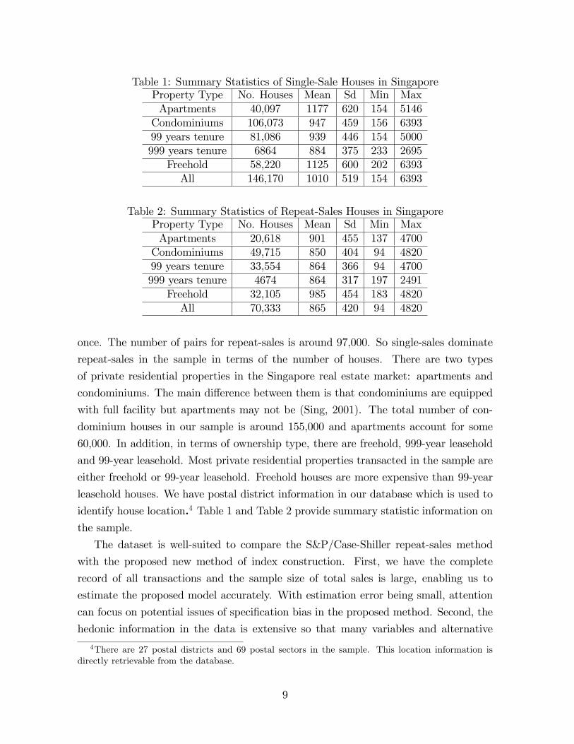
Table 1: Summary Statistics of Single-Sale Houses in SingaporeProperty Type No. Houses Mean Sd Min MaxApartments 40,097 1177 620 154 5146Condominiums 106,073 947 459 156 639399 years tenure 81,086 939 446 154 5000999 years tenure 6864 884 375 233 2695

Freehold 58,220 1125 600 202 6393All 146,170 1010 519 154 6393

Table 2: Summary Statistics of Repeat-Sales Houses in SingaporeProperty Type No. Houses Mean Sd Min MaxApartments 20,618 901 455 137 4700Condominiums 49,715 850 404 94 482099 years tenure 33,554 864 366 94 4700999 years tenure 4674 864 317 197 2491

Freehold 32,105 985 454 183 4820All 70,333 865 420 94 4820

once. The number of pairs for repeat-sales is around 97,000. So single-sales dominate

repeat-sales in the sample in terms of the number of houses. There are two types

of private residential properties in the Singapore real estate market: apartments and

condominiums. The main difference between them is that condominiums are equipped

with full facility but apartments may not be (Sing, 2001). The total number of con-

dominium houses in our sample is around 155,000 and apartments account for some

60,000. In addition, in terms of ownership type, there are freehold, 999-year leasehold

and 99-year leasehold. Most private residential properties transacted in the sample are

either freehold or 99-year leasehold. Freehold houses are more expensive than 99-year

leasehold houses. We have postal district information in our database which is used to

identify house location.4 Table 1 and Table 2 provide summary statistic information onthe sample.

The dataset is well-suited to compare the S&P/Case-Shiller repeat-sales method

with the proposed new method of index construction. First, we have the complete

record of all transactions and the sample size of total sales is large, enabling us to

estimate the proposed model accurately. With estimation error being small, attention

can focus on potential issues of specification bias in the proposed method. Second, the

hedonic information in the data is extensive so that many variables and alternative

4There are 27 postal districts and 69 postal sectors in the sample. This location information isdirectly retrievable from the database.

9

Figure 1: Scatter plots of house prices per square foot over January 1995 - June 2014

specifications can be included on the right hand side of the model (1). Third, there are

a very large number of repeat sales in the data, so that model (4) can also be estimated

accurately. Consequently, we can again ignore estimation error and focus on potential

sample selection bias in the repeat-sales method.

It is worth noting that single-sale properties display different summary statistics

from repeat-sales properties. The mean price and the standard deviation for repeat-

sales houses is lower than single-sales houses across all categories. This observation

supports the argument that repeat-sales houses are not a representative random sample

of the entire market and carry a potential sample selection bias. Furthermore, in spite

of the long sample period, about 68% of houses in the sample that have changed hands

are single-sales houses. So the repeat-sale method is based on only about 32% of the

houses in the sample.

The scatter plot of all house prices per square foot over time is given in Figure 1.

It is diffi cult to discern the price trend from this scatter plot, especially for houses at

the low-end of the market. For the high-end houses, prices seem to be stable between

2000 and 2006.

To fit the model in equation (8), we take account of the following three property

characteristics: location, property type, and ownership type. We use postal district

information in our database to identify a house location. The real estate price index is

βt, the quarterly index from Q1 1995 to Q2 2014 (78 quarters in total). In addition,

there are two types of properties (apartments and condominiums) and three types of

ownership (99 years, 999 years, and freehold). Taking these features of the data into

account, equation (1) may be rewritten as

10

yi,j,z = βt(i,j,z) + γ1X(1)i,z + γ2X

(2)i,z + γ3X

(3)i,z + µz + hi,z + εi,j,z,

where X(1)i,z is equal to 1 when the property type is condominium and 0 when it is an

apartment. Similarly, we construct two other dummy variables as

X(2)i,z =

{1 if 999 lease0 if otherwise

,

X(3)i,z =

{1 if freehold0 if otherwise

.

Although we only use the three dummy variables in our empirical analysis, the model

can be easily expanded to include additional hedonic information as covariates. We

have experimented with other covariates and the main empirical findings reported here

are qualitatively unchanged. For simplicity, therefore, we report results with the above

specification.

We first fit the model to all data (named the Group Averaging for all sales) and

obtain βt. We also fit the model to the data that contain single sales only (named

the Group Averaging for single sales) and obtain βt. Since our purpose is to construct

the house price index instead of its logarithm, following Nagaraja, Brown and Zhao

(2011), we calculate It = exp(βt).5 Finally, we take the first quarter in our sample as

the reference point where the price index is set to unity.

For comparison, we also apply the S&P/Case-Shiller method to repeat-sales prices

to build the index. We plot the two indices from the proposed group averaging method,

the S&P/Case-Shiller index, and the price index published by Urban Redevelopment

Authority (URA) in Figure 2.6 It is obvious that all three indices are similar over the

period 1995-2007 at which point they start to differ noticeably. The differences becomes

more pronounced after 2010.

To compare the quality of the two indices from the proposed group averaging method

and the S&P/Case-Shiller index, we examine their out-of-sample predictive power. To

do so, we divide the observations into training and testing datasets. The testing set

contains all the final sales of the houses sold three or more times in our sample period.

Among the houses sold twice, their second transactions are randomly put into the

testing set with probability 0.05. We also randomly add single-sale houses into our

5Although It is biased downward for It, the biased corrected estimator leads to virtually no changeto our results since the estimation error (and hence the variance estimate that appears in the biascalculation) is small.

6Since the exact methodology of URA is not entirely clear to us, we cannot use it for out-of-samplepredictions.

11

Figure 2: The Real Estate Price Indices for Singapore: Q1 1995 —Q2 2014

testing set with probability 0.16 so that the testing set contains the same number of

single-sale houses and repeat-sales ones. All the remaining houses are included in the

training set. The resulting testing set contains around 15% of sales in our sample, of

which 50% are single-sale houses and the rest are repeat-sales.

We first estimate the indices on the training set by the different modeling methods

and then examine their out-of-sample forecasts on the testing set. To calculate the

estimated price for the repeat-sales homes in the testing set, we use

Yt′,i =It′

ItYt,i,

where Yt,i is the price per square foot for house i at time t, t′ > t and It is the estimated

index at time t. To calculate the estimated price for the single-sale homes, we use

Yi,z =It(i,z)It(i,z)−1

Yt(i,z)−1,

where t(i, z) is the transaction period for house i at area z,7 Yt(i,z)−1 is the average price

per square foot for area z at time t(i, z) − 1 and It(i,z) is the estimated index at time

t(i, z).

7For single-sale houses, we simply write t(i, 1, z) as t(i, z).

12

Figure 3: Three real estate price indices and the dates of ten rounds of successivemacroprudential cooling measures.

The RMSE results are shown in Table 3.8 The S&P/Case-Shiller index clearly has

the best predictive power for repeat-sales homes, whereas our Group Averaging indices

perform (marginally) better for single-sale houses. However, after we use all sales in the

testing set for forecasting, we find that the S&P/Case-Shiller index performs best since

the S&P/Case-Shiller index performs so much better in predicting the price of repeat-

sales houses but only slightly worse than the Group Averaging indices when forecasting

the price of single-sale homes.

As discussed, it is known that the repeat-sales method is subject to sample selection

bias. Our data indicate that repeat-sales houses are different from single-sale houses.

Although this difference is a principal argument advanced for using hedonic models,

the empirical results found here suggest a preference for using the repeat sales method.

The results in Table 3 indicate that the specification error in hedonic models outweighs

their advantage in removing the sample selection bias of the repeat-sales method.

8We have also tried using tenure length and house type (apartment versus condominium) in pre-dicting prices. But the RMSEs of forecast only change by a small amount.

13

Table 3: Testing set RMSE for the Indices (SG dollars)Test Set S&P/C-S G.A. (all sales) G.A. (single sale)Single sales 285.8 279.5 280.0Repeat sales 196.9 278.8 303.9All sales 245.4 279.1 292.2

Figure 4: The S&P/Case-Shiller index, the BSADF statistic of PSY and the criticalvalues.

4 Cooling Measures and Explosive Behavior

Housing is a highly important sector of the economy and provides the largest form of

savings of household wealth in Singapore. Property prices play an important role in

consumer price inflation and can therefore have a serious impact on public policy. The

private housing sector, property prices and rents also impact measures of Singapore’s

competitiveness in the world economy. For these and other reasons, the Singapore

government has closely watched movements in housing prices over the last decade and

particularly since the house price bubble in the USA. Recently, Singapore implemented

ten successive rounds of macro-prudential measures intended to cool down the housing

market. These measures were undertaken between September 2009 and December 2013,

the first eight of which were targeted directly at the private residential market.

The Appendix summarizes the dates and the nature of these macro-prudential mea-

14

sures. As is evident, a variety of macro-prudential policies have been used by the

Singapore government. These include introducing a Seller’s Stamp Duty (SSD), low-

ering the Loan-to-Value (LTV) limit, introducing an Additional Buyer’s Stamp Duty

(ABSD), and reducing the Total Debt Servicing Ratio (TDSR) and the Mortgage Ser-

vicing Ratio (MSR). To visualize the impact of these cooling measures on the dynamics

of real estate price movements, Figure 3 plots the three price indices for the period be-

tween Q1 2008 and Q2 2014, superimposed by vertical lines indicating the introduction

of these ten cooling measures.

The primary goal of the macro-prudential policies is to reduce or eliminate emergent

price bubbles in the real estate market and bring prices closer in line with fundamental

values. Using the present value model, Diba and Grossman (1988) showed the presence

of a rational bubble solution that implies that an explosive behavior in the observed

price. If fundamental values are not explosive, then the explosive behavior in prices

is a suffi cient condition for the presence of bubble. Phillips, Wu and Yu (2011) and

Phillips, Shi and Yu (2014a, 2014b, PSY hereafter) introduced recursive and rolling

window econometric methods to test for the presence of mildly explosive behavior or

market exuberance in financial asset prices. These methods also facilitated estimation

of the origination and termination dates of explosive bubble behavior. The method

of Phillips, Wu and Yu (2011) is particularly effective when there is a single explosive

episode in the data while the method of PSY can identify multiple explosive episodes.

In the absence of prior knowledge concerning the number of explosive episodes, in what

follows we use the PSY method to assess evidence of bubbles in real estate prices.

Bubble behavior and market exuberance and collapse are subsample phenomena.

So, PSY proposed the use of rolling window recursive application of right sided unit

root tests (against explosive alternatives) using a fitted model for data {Xt}nt=1 of thefollowing form

∆Xt = α + βXt−1 +K∑i=1

βi∆Xt−i + et. (10)

Details of the procedure and its asymptotic properties are given in PSY. We provide

a synopsis here and refer readers to PSY for further information about the specifics

of implementation and the procedure properties. Briefly, the unit root test recursion

involves a sequence of moving windows of data in the overall sample that expands

backward from each observation t = bnrc of interest, where n is the sample size andbnrc denotes the integer part of nr for r ∈ [0, 1]. Let r1 and r2 denote the start and end

point fractions of the subsample regression. The resulting sequence of calculated unit

root test statistics are denoted as{ADF r2

r1

}r1∈[0,r2−r0]

where r0 is the minimum window

15

Figure 5: Testing for Bubbles in Singapore Real Estate Prices: using the Group averageindex (all sales), the BSADF statistic of PSY and critical values of the test recursion.

size used in the recursion. and t = bTrc is the point in time for which we intend totest for normal market behavior against exuberance. PSY define the recursive statistic

BSADFr = supr1∈[0,r2−r0],r2=r{ADF r2

r1

}. The origination and termination dates of an

explosive period are then determined from the crossing times

re = infr∈[r0,1]

{r : BSADFr > cv} and rf = infr∈[re,1]

{r : BSADFr < cv} , (11)

where the recursive statistic BSADF crosses its critical value cv. The quantity re es-

timates the origination date of an explosive period and rf estimates the termination

date of an explosive period. After the first explosive period is identified, the same

method may be used to identify origination and termination dates of subsequent explo-

sive episodes in the data.

To assess evidence for potential bubbles in the private real estate market in Singa-

pore, we applied the PSY method first to the S&P/Case-Shiller index with minimum

rolling window size r0 = 8, corresponding to two years. Figure 4 reports the index,

the BSADF statistics and the 5% critical values. The shaded area corresponds to

the explosive period where the BSADF statistic exceeds the critical value. The PSY

method identifies an explosive period, namely Q4 2006 to Q1 2008, in the data. During

this period, no cooling measures were introduced by the government. If the government

16

had been alerted to the existence of exuberant market conditions in real time during

this period, the opportunity would have been available for the implementation of cool-

ing measures to affect the market. Moreover, although all three indices suggest that

there were upward movements in price following 2008, between 2009 and 2013, these

movements are not determined to be explosive and he PSY detector indicates little

or no evidence of explosive behavior after 2009. This tapering in real estate market

exuberance coincides with period September 2009 and December 2013 in which the

macro-prudential cooling measures were undertaken by the government.

We also applied the PSYmethod to the Group Average all-sales index with minimum

rolling window size r0 = 8. Figure 5 reports the index, the test recursion, and the test

5% critical values. The empirical results for this series mirror those for the S&P/Case-

Shiller index, confirming the findings of a bubble in the private real estate market over

Q1 2007 to Q1 2008.

5 Conclusion

In order to exploit all available information in real estate markets, this paper provides

a new hedonic model for the estimation of real estate price indices. The new model

has the advantage of using both single-sales and repeat-sales data and is less prone

to misspecification bias than standard hedonic models and less prone to selection bias

than repeat-sales methods that use only partial data sets. The model is also easy

to estimate. Unlike the maximum likelihood methods of Hill, Knight and Sirmans

(1997) and Nagaraja, Brown and Zhao (2011), this approach uses ordinary least square

estimation and is computationally effi cient with large datasets.

We apply our estimation procedure to the real estate market for private residential

dwellings in Singapore and examine the model’s out-of-sample predictive performance

in comparison with indices produced using the repeat-sales methodology of Case and

Shiller (1987, 1988). The findings reveal that, compared with the repeat-sales methodol-

ogy, our method performs better at forecasting prices of single-sale homes, but worse at

forecasting prices of repeat-sales houses. When taking into account all sales in the fore-

cast comparison, we find that Case-Shiller has superior predictive performance, echoing

Shiller’s (2008) maxim that “the repeat-sales method is the only way to go”by Shiller

(2008).

The recursive detection method of Phillips, Shi and Yu (2014a) is applied to each

of the indices to locate episodes of real estate price exuberance in Singapore. Only one

explosive period in the indices, from Q1 2007 to Q1 2008, is detected. Although all

17

the indices grew during 2009 - 2013, the expansion is not explosive, indicating that ten

recent rounds of cooling measure intervention in the real estate market by the Singapore

government have been successful in controlling prices.

Appendix

Dates and the content of recent real estate market cooling mea-sures introduced in Singapore.

1. 2009/9/14

• Reinstatement of the confirmed list for the 1st half 2010 government landsales programme

• Removal of the interest absorption scheme and interest-only housing loans

• Non-extension of the January 2009 budget assistance measures for the prop-erty market

2. 2010/2/20

• Introduction of a Seller’s Stamp Duty (SSD) on all residential properties andlands sold within one year of purchase

• Loan-to-Value (LTV) limit lowered from 90% to 80% for all housing loans

3. 2010/8/30

• Holding period for imposition of SSD increased from one year to three years

• Minimum cash payment increased from 5% to 10% and the LTV limit de-

creased to 70% for buyers with one or more outstanding housing loans

• The extended SSD does not affect HDB lessees as the required Minimum

Occupation Period for HDB flats is at least 3 years

4. 2011/1/14

• Increase the holding period for imposition of SSD from three years to four

years

• Raise SSD rates to 16%, 12%, 8% and 4% for residential properties sold in

the first, second, third and fourth year of purchase respectively

18

• Lower the LTV limit to 50% on housing loans for property purchasers who

are not individuals

• Lower the LTV limit on housing loans from 70% to 60% for second property

5. 2011/12/8

• Introduction of an Additional Buyer’s Stamp Duty (ABSD)

• Developers purchasing more than four residential units and following throughon intention to develop residential properties for sale would be waived ABSD

6. 2012/10/6

• Mortgage tenures capped at a maximum of 35 years

• For loans longer than 30 years or for loans that extend beyond retirement ageof 65 years: LTV lowered to 60% for first mortgage and to 40% for second

and subsequent mortgages

• LTV for non-individuals lowered to 40%

7. 2013/1/12

• Higher ABSD rates

• Decrease the LTV limit for second/third loan to 50/40% from 60%; non-

individuals’LTV to 20% from 40%

• Mortgage Servicing Ratio (MSR) for HDB loans now capped at 35% of

gross monthly income (from 40%); MSR for loans from financial institutions

capped at 30%

8. 2013/6/28: Introduction of Total Debt Servicing Ratio (TDSR). The total monthly

repayments of debt obligations should not exceed 60% of gross monthly income.

9. 2013/8/27

• Singapore Permanent Resident (SPR) Households need to wait three years,before they can buy a resale HDB flat

• Maximum tenure for HDB housing loans is reduced to 25 years. The MSR

limit is reduced to 30% of the borrower’s gross monthly income

19

• Maximum tenure of new housing loans and re-financing facilities for the pur-chase of HDB flats is reduced to 30 years. New loans with tenure exceeding

25 years and up to 30 years will be subject to tighter LTV limits

10. 2013/12/9

• Reduction of cancellation fees From 20% to 5% for executive condominiums

• Resale levy for second-timer applicants

• Revision of mortgage loan terms. Decrease MSR from 60% to 30% of a

borrower’s gross monthly income

References

[1] Bailey, Martin J., Richard F. M., and H. O. Nourse. “A regression method for real

estate price index construction.”Journal of the American Statistical Association

58.304 (1963): 933-942.

[2] Case, B., H. O. Pollakowski, and S. M. Wachter. “On choosing among house price

index methodologies.”Real Estate Economics 19.3 (1991): 286-307.

[3] Case, B., and J. M. Quigley. “The dynamics of real estate prices.”The Review of

Economics and Statistics (1991): 50-58.

[4] Case, K. E., and R. Shiller. “Prices of single-family homes since 1970: New indexes

for four cities.”New England Economic Review (1987): 45-56.

[5] Case, K. E., and R. J. Shiller. “The Effi ciency of the Market for Single-Family

Homes.”The American Economic Review (1989): 125-137.

[6] Clapp, J. M., C. Giaccotto, and D. Tirtiroglu. “Housing price indices based on all

transactions compared to repeat subsamples.”Real Estate Economics 19.3 (1991):

270-285.

[7] Diba, Behzad T., and Herschel I. Grossman. “Explosive rational bubbles in stock

prices?.”The American Economic Review (1988): 520-530.

[8] Englund, P., J. M. Quigley, and C. L. Redfearn. “Improved price indexes for real

estate: measuring the course of Swedish housing prices.” Journal of Urban Eco-

nomics 44.2 (1998): 171-196.

20

[9] Hill, R. Carter, John R. Knight, and C. F. Sirmans. “Estimating capital asset price

indexes.”Review of Economics and Statistics 79.2 (1997): 226-233.

[10] Hill, R. C., C. F. Sirmans, and J. R. Knight. “A random walk down main street?”

Regional Science and Urban Economics 29.1 (1999): 89-103.

[11] Hwang, M., and J. M. Quigley. “Housing price dynamics in time and space: pre-

dictability, liquidity and investor returns.”The Journal of Real Estate Finance and

Economics 41.1 (2010): 3-23.

[12] Gatzlaff, D. H., and D. R. Haurin. “Sample selection bias and repeat-sales index

estimates.”The Journal of Real Estate Finance and Economics 14.1-2 (1997): 33-

50

[13] Ghysels, E., A. Plazzi, W. N. Torous, and R. Valkanov. “Forecasting real estate

prices.”Handbook of Economic Forecasting 2 (2012).

[14] Guo, X.., Zheng, S.., Geltner, D., and Liu, H. “A New Approach for Constructing

Home Price Indices in China: The Pseudo Repeat Sales Model.”Journal of Housing

Economics (2014): 20-38.

[15] Nagaraja, C. H., L. D. Brown, and L. H. Zhao. “An autoregressive approach to

house price modeling.”The Annals of Applied Statistics 5.1 (2011): 124-149.

[16] Phillips, P. C. B., S. Shi, and J. Yu. “Testing for multiple bubbles: Historical

episodes of exuberance and collapse in the S&P 500.” International Economic

Review, forthcoming (2014a).

[17] Phillips, P. C. B., S. Shi, and J. Yu. “Testing for Multiple Bubbles: Limit Theory

of Real Time Detector,”International Economic Review, forthcoming (2014b)

[18] Phillips, P. C. B., Wu, Y., and J. Yu, “Explosive behavior in the 1990s Nasdaq:

When did exuberance escalate asset values?” International Economic Review, 52

(2011):201—226.

[19] Quigley, J. M. “A simple hybrid model for estimating real estate price indexes.”

Journal of Housing Economics 4.1 (1995): 1-12.

[20] Shiller, R. J. “Derivatives markets for home prices.”No. w13962. National Bureau

of Economic Research, 2008.

21

[21] Rosen, S.. “Hedonic prices and implicit markets: Product differentiation in pure

competition.”Journal of Political Economy 82.1 (1974): 34-55.

[22] Sing, T.. “Dynamics of the condominium market in Singapore.”International Real

Estate Review 4.1 (2001): 135-158.

[23] Basket-based Property Price Indexes for Singapore Non-landed Private Residential

Properties (March. 2010), www.ires.nus.edu.sg

[24] S&P/Case-Shiller Home Price Indices-Index Methodology (Nov. 2009)

http://www.standardandpoors.com/

22