A New Digital Filter Using Window Resizing for Protective Relay Applications

Bogdan Kasztenny, Mangapathirao V. Mynam, Titiksha Joshi, and Chad Daniels Schweitzer Engineering Laboratories, Inc.

Published in the proceedings of the 15th International Conference

on Developments in Power System Protection Liverpool, United Kingdom

March 9–12, 2020

1

A NEW DIGITAL FILTER USING WINDOW RESIZING FOR PROTECTIVE RELAY APPLICATIONS

Bogdan Kasztenny1*, Mangapathirao V. Mynam1, Titiksha Joshi1, Chad Daniels1

1Schweitzer Engineering Laboratories, Inc., Pullman, Washington, USA *bogdan_kasztenny@selinc.com

Keywords: POWER SYSTEM PROTECTION, VARIABLE-WINDOW FILTER, WINDOW RESIZING.

Abstract

Digital protective relays use finite impulse response filters with sliding data windows for band-pass filtering of voltages and currents and measurement of phasors. Cosine, Fourier, and Walsh data windows are commonly used. Short windows yield faster protection operation but allow larger transient errors jeopardizing protection security and calling for adequate countermeasures. Often, these countermeasures erase some, if not most, benefits of shorter data windows. This paper presents the theory, implementation, laboratory test results, and a field case example of a new filtering method for protective relaying based on window resizing. The method uses a full-cycle sliding data window until a disturbance is detected, at which time the window size is considerably shortened to include only disturbance samples and exclude all pre-disturbance samples. With passing of time, the window size grows to include more disturbance samples as they become available. When the window reaches its nominal full-cycle size, it stops extending and starts sliding again. By purging the pre-disturbance data, the new filter strikes an excellent balance between speed and accuracy. We derive the method for fixed sampling and processing rates and include compensation for frequency deviations in the input signals.

1 Introduction

Recently, new implementations of protection elements and schemes became available that are based on superimposed components and traveling waves [1] and operate on the order of 2 ms. These protection principles work on fault-induced signals supplied not only by the sources but also with the energy stored in the network prior to the fault. This reduced dependence on power sources makes them a viable solution for protection applications near non-traditional power sources. However, transient-based protection methods are not fully dependable because traveling waves dissipate, and incremental quantities expire. Therefore, transient-based protection elements and schemes need a dependable backup.

Dependable protection elements and schemes must work on the same signal spectrum as the power sources that drive fault currents in the grid. Modern power grids with high penetration of wind generators, inverters, and static condensers supply fault currents only for a short time. Therefore, backup for transient-based protection must not only be dependable, but also fast. Considering non-traditional power sources, protection speed is an important way to improve dependability.

Historically, protective relays use band-pass filters to obtain protection operating signals consistent with the frequency of fault currents and voltages, while rejecting other signal components (phasor-based protection). Since the beginning of protective relaying, relay filter designers have strived to address the contradicting requirements of speed (short group delay of the filters) and security (accurate measurement through rejection of the out-of-band signal components).

Digital protective relays use finite impulse response (FIR) filters with sliding data windows for band-pass filtering and measurement of phasors. Cosine, Fourier, and Walsh data windows are commonly used. Short windows yield faster operation but allow larger transient errors. Often, intentional delay, reduced reach, or additional restraining in general, are used in the protection logic to address these transient errors. This, however, partially or entirely, erases the initial gain of speed and makes the design ineffective. In some cases, two parallel measurement paths are used, such as with full-cycle and half-cycle (or even quarter-cycle) filters operating in parallel. The full-cycle measurement is slower but dependable. The measurement with a shorter data window is faster, but it may be intentionally desensitized and may operate only under certain favorable conditions.

This paper presents the theory, implementation, laboratory test results, and a field case example of a new filtering method that uses filter window resizing to achieve the following:

• Speed of operation. • Accuracy of the operating characteristics. • Efficiency of implementation.

The highlights of the new method include the following:

• The filter window resizes to a short length upon detecting a disturbance. The new window subsequently grows with each new available sample and eventually slides after reaching its full nominal length.

• The filter includes a carefully designed resizing logic to allow or prevent resizing for optimum performance while maintaining security.

2

• Instead of letting the window slide from the pre-fault state to the fault state, the algorithm intentionally delays window resizing for a few milliseconds so that the pre-disturbance data are entirely purged from the filter window. Hence, the shortened window contains only the fault state data, which provides good accuracy, despite using a short data window following resizing.

• The method can be used as a plain filter, and therefore it may be combined with any other post-processing algorithm, such as a pair of orthogonal filters for phasor estimation. Or, the method can be used directly to measure phasors.

• The method is applicable to protection elements and schemes that use fundamental-frequency measurements across all protection applications.

• The method is derived for a relay hardware with a fixed sampling rate, and an arbitrary fixed processing rate.

• The method compensates for off-nominal frequency of the inputs and for the group delay, allowing the downstream protection logic to compare the input samples with the filter output samples, if desired.

The presented method has been implemented in relay hardware and this paper shows results from testing a physical device.

2 Filter Window Resizing

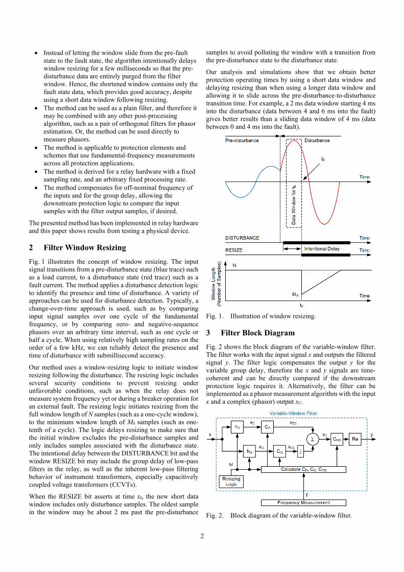
Fig. 1 illustrates the concept of window resizing. The input signal transitions from a pre-disturbance state (blue trace) such as a load current, to a disturbance state (red trace) such as a fault current. The method applies a disturbance detection logic to identify the presence and time of disturbance. A variety of approaches can be used for disturbance detection. Typically, a change-over-time approach is used, such as by comparing input signal samples over one cycle of the fundamental frequency, or by comparing zero- and negative-sequence phasors over an arbitrary time interval, such as one cycle or half a cycle. When using relatively high sampling rates on the order of a few kHz, we can reliably detect the presence and time of disturbance with submillisecond accuracy.

Our method uses a window-resizing logic to initiate window resizing following the disturbance. The resizing logic includes several security conditions to prevent resizing under unfavorable conditions, such as when the relay does not measure system frequency yet or during a breaker operation for an external fault. The resizing logic initiates resizing from the full window length of N samples (such as a one-cycle window), to the minimum window length of M0 samples (such as one-tenth of a cycle). The logic delays resizing to make sure that the initial window excludes the pre-disturbance samples and only includes samples associated with the disturbance state. The intentional delay between the DISTURBANCE bit and the window RESIZE bit may include the group delay of low-pass filters in the relay, as well as the inherent low-pass filtering behavior of instrument transformers, especially capacitively coupled voltage transformers (CCVTs).

When the RESIZE bit asserts at time t0, the new short data window includes only disturbance samples. The oldest sample in the window may be about 2 ms past the pre-disturbance

samples to avoid polluting the window with a transition from the pre-disturbance state to the disturbance state.

Our analysis and simulations show that we obtain better protection operating times by using a short data window and delaying resizing than when using a longer data window and allowing it to slide across the pre-disturbance-to-disturbance transition time. For example, a 2 ms data window starting 4 ms into the disturbance (data between 4 and 6 ms into the fault) gives better results than a sliding data window of 4 ms (data between 0 and 4 ms into the fault).

Fig. 1. Illustration of window resizing.

3 Filter Block Diagram

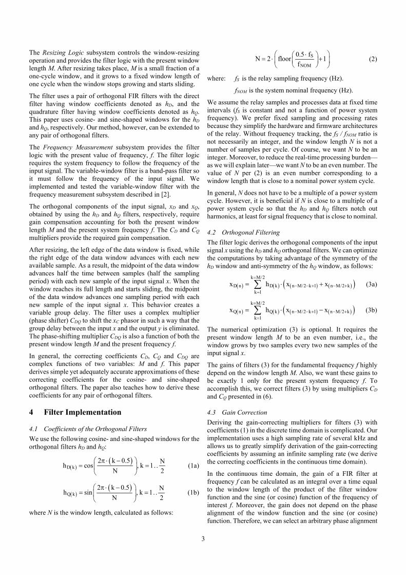
Fig. 2 shows the block diagram of the variable-window filter. The filter works with the input signal x and outputs the filtered signal y. The filter logic compensates the output y for the variable group delay, therefore the x and y signals are time-coherent and can be directly compared if the downstream protection logic requires it. Alternatively, the filter can be implemented as a phasor measurement algorithm with the input x and a complex (phasor) output xC.

Fig. 2. Block diagram of the variable-window filter.

3

The Resizing Logic subsystem controls the window-resizing operation and provides the filter logic with the present window length M. After resizing takes place, M is a small fraction of a one-cycle window, and it grows to a fixed window length of one cycle when the window stops growing and starts sliding.

The filter uses a pair of orthogonal FIR filters with the direct filter having window coefficients denoted as hD, and the quadrature filter having window coefficients denoted as hQ. This paper uses cosine- and sine-shaped windows for the hD and hQ, respectively. Our method, however, can be extended to any pair of orthogonal filters.

The Frequency Measurement subsystem provides the filter logic with the present value of frequency, f. The filter logic requires the system frequency to follow the frequency of the input signal. The variable-window filter is a band-pass filter so it must follow the frequency of the input signal. We implemented and tested the variable-window filter with the frequency measurement subsystem described in [2].

The orthogonal components of the input signal, xD and xQ, obtained by using the hD and hQ filters, respectively, require gain compensation accounting for both the present window length M and the present system frequency f. The CD and CQ multipliers provide the required gain compensation.

After resizing, the left edge of the data window is fixed, while the right edge of the data window advances with each new available sample. As a result, the midpoint of the data window advances half the time between samples (half the sampling period) with each new sample of the input signal x. When the window reaches its full length and starts sliding, the midpoint of the data window advances one sampling period with each new sample of the input signal x. This behavior creates a variable group delay. The filter uses a complex multiplier (phase shifter) CDQ to shift the xC phasor in such a way that the group delay between the input x and the output y is eliminated. The phase-shifting multiplier CDQ is also a function of both the present window length M and the present frequency f.

In general, the correcting coefficients CD, CQ and CDQ are complex functions of two variables: M and f. This paper derives simple yet adequately accurate approximations of these correcting coefficients for the cosine- and sine-shaped orthogonal filters. The paper also teaches how to derive these coefficients for any pair of orthogonal filters.

4 Filter Implementation

4.1 Coefficients of the Orthogonal Filters We use the following cosine- and sine-shaped windows for the orthogonal filters hD and hQ:

( )( )

D k2 k 0.5 Nh cos , k 1. .

N 2π ⋅ −

= =

(1a)

( )( )

Q k2 k 0.5 Nh sin , k 1. .

N 2π ⋅ −

= =

(1b)

where N is the window length, calculated as follows:

S

NOM

0.5 fN 2 floor 1f

⋅ = ⋅ +

(2)

where: fS is the relay sampling frequency (Hz).

fNOM is the system nominal frequency (Hz).

We assume the relay samples and processes data at fixed time intervals (fS is constant and not a function of power system frequency). We prefer fixed sampling and processing rates because they simplify the hardware and firmware architectures of the relay. Without frequency tracking, the fS / fNOM ratio is not necessarily an integer, and the window length N is not a number of samples per cycle. Of course, we want N to be an integer. Moreover, to reduce the real-time processing burden—as we will explain later—we want N to be an even number. The value of N per (2) is an even number corresponding to a window length that is close to a nominal power system cycle.

In general, N does not have to be a multiple of a power system cycle. However, it is beneficial if N is close to a multiple of a power system cycle so that the hD and hQ filters notch out harmonics, at least for signal frequency that is close to nominal.

4.2 Orthogonal Filtering The filter logic derives the orthogonal components of the input signal x using the hD and hQ orthogonal filters. We can optimize the computations by taking advantage of the symmetry of the hD window and anti-symmetry of the hQ window, as follows:

( ) ( ) ( ) ( )( )k M/2

D n D k n M/2 k 1 n M/2 kk 1

x h x x=

− − + − +=

= ⋅ +∑ (3a)

( ) ( ) ( ) ( )( )k M/2

Q n Q k n M/2 k 1 n M/2 kk 1

x h x x=

− − + − +=

= ⋅ −∑ (3b)

The numerical optimization (3) is optional. It requires the present window length M to be an even number, i.e., the window grows by two samples every two new samples of the input signal x.

The gains of filters (3) for the fundamental frequency f highly depend on the window length M. Also, we want these gains to be exactly 1 only for the present system frequency f. To accomplish this, we correct filters (3) by using multipliers CD and CQ presented in (6).

4.3 Gain Correction Deriving the gain-correcting multipliers for filters (3) with coefficients (1) in the discrete time domain is complicated. Our implementation uses a high sampling rate of several kHz and allows us to greatly simplify derivation of the gain-correcting coefficients by assuming an infinite sampling rate (we derive the correcting coefficients in the continuous time domain).

In the continuous time domain, the gain of a FIR filter at frequency f can be calculated as an integral over a time equal to the window length of the product of the filter window function and the sine (or cosine) function of the frequency of interest f. Moreover, the gain does not depend on the phase alignment of the window function and the sine (or cosine) function. Therefore, we can select an arbitrary phase alignment

4

that gives us the simplest integral to solve. We can also select either a sine or cosine function, depending on which function is easier to solve.

Following the above approach, we can obtain the continuous time-domain approximation of the gain coefficients as follows:

( ) ( )

MN

1D D

NOMMN

fC h z cos z dzf

π−

− π

= ⋅ ⋅ ∫ (4a)

( ) ( )

MN

1Q Q

NOMMN

fC h z sin z dzf

π−

− π

= ⋅ ⋅ ∫ (4b)

Equations (4) apply to any pair of orthogonal filters. For the orthogonal filters (2) we write the following:

( ) ( )

MN

1D

NOMMN

fC cos z cos z dzf

π−

− π

= ⋅ ⋅ ∫ (5a)

( ) ( )

MN

1Q

NOMMN

fC sin z sin z dzf

π−

− π

= ⋅ ⋅ ∫ (5b)

Equations (5) are straightforward to solve and yield the following gain-correcting coefficients:

( ) ( ) 1

Dsin A sin BMC

2 A B

−

= ⋅ + (6a)

( ) ( ) 1

Qsin A sin BMC

2 A B

−

= ⋅ − (6b)

where:

NOM

M fA 1N f

= π ⋅ ⋅ −

(6c)

NOM

M fB 1N f

= π ⋅ ⋅ +

(6d)

The value of A approaches 0 when the system operates near the nominal frequency. Of course, sin(A) / A in (6a) and (6b) approaches 1 if A approaches 0.

Equations (6) show us that the gain-correcting coefficients depend on the per-unit system frequency f / fNOM, the present per-unit window length M / N, and the present window length in samples, M. System frequency does not change fast, and the f / fNOM value can be refreshed relatively slowly. The rest of the operations involved in (6) can be implemented through a combination of real-time calculations and look-up tables.

As expected, the gain-correcting coefficients do not depend on the relay sampling frequency fS because we derived these coefficients as approximations in the continuous time domain.

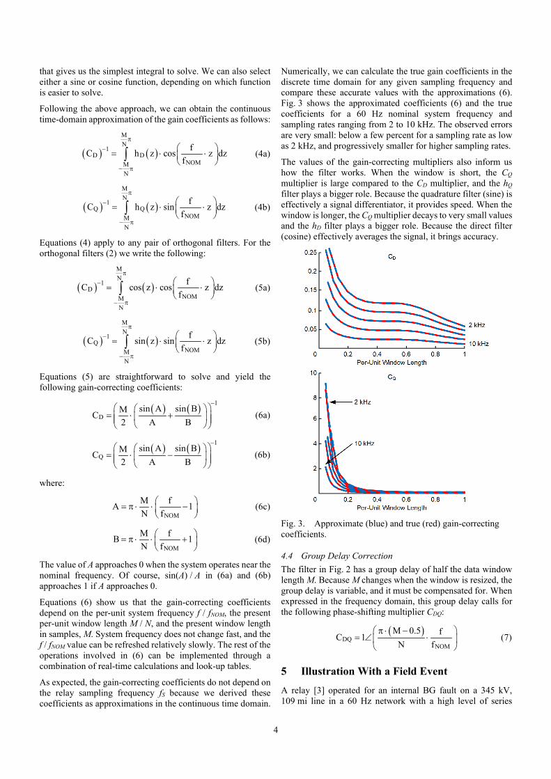
Numerically, we can calculate the true gain coefficients in the discrete time domain for any given sampling frequency and compare these accurate values with the approximations (6). Fig. 3 shows the approximated coefficients (6) and the true coefficients for a 60 Hz nominal system frequency and sampling rates ranging from 2 to 10 kHz. The observed errors are very small: below a few percent for a sampling rate as low as 2 kHz, and progressively smaller for higher sampling rates.

The values of the gain-correcting multipliers also inform us how the filter works. When the window is short, the CQ multiplier is large compared to the CD multiplier, and the hQ filter plays a bigger role. Because the quadrature filter (sine) is effectively a signal differentiator, it provides speed. When the window is longer, the CQ multiplier decays to very small values and the hD filter plays a bigger role. Because the direct filter (cosine) effectively averages the signal, it brings accuracy.

Fig. 3. Approximate (blue) and true (red) gain-correcting coefficients.

4.4 Group Delay Correction The filter in Fig. 2 has a group delay of half the data window length M. Because M changes when the window is resized, the group delay is variable, and it must be compensated for. When expressed in the frequency domain, this group delay calls for the following phase-shifting multiplier CDQ:

( )DQ

NOM

M 0.5 fC 1N f

π ⋅ − = ∠ ⋅

(7)

5 Illustration With a Field Event

A relay [3] operated for an internal BG fault on a 345 kV, 109 mi line in a 60 Hz network with a high level of series

5

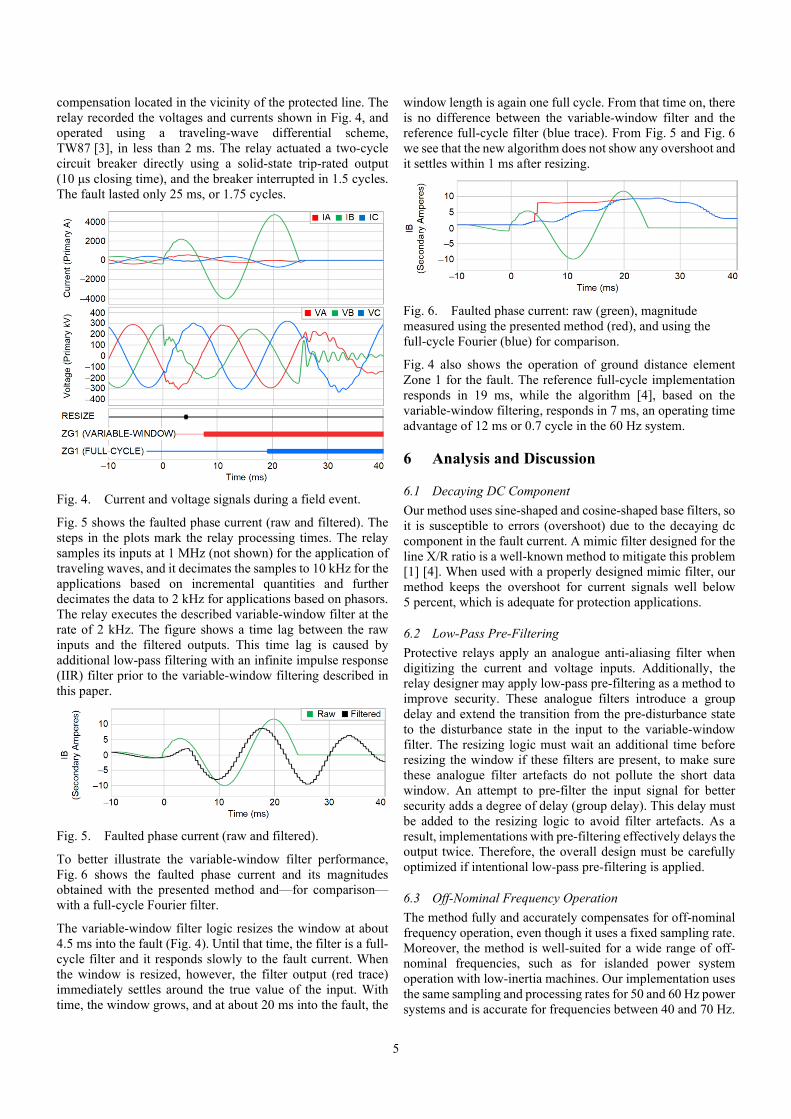
compensation located in the vicinity of the protected line. The relay recorded the voltages and currents shown in Fig. 4, and operated using a traveling-wave differential scheme, TW87 [3], in less than 2 ms. The relay actuated a two-cycle circuit breaker directly using a solid-state trip-rated output (10 μs closing time), and the breaker interrupted in 1.5 cycles. The fault lasted only 25 ms, or 1.75 cycles.

Fig. 4. Current and voltage signals during a field event.

Fig. 5 shows the faulted phase current (raw and filtered). The steps in the plots mark the relay processing times. The relay samples its inputs at 1 MHz (not shown) for the application of traveling waves, and it decimates the samples to 10 kHz for the applications based on incremental quantities and further decimates the data to 2 kHz for applications based on phasors. The relay executes the described variable-window filter at the rate of 2 kHz. The figure shows a time lag between the raw inputs and the filtered outputs. This time lag is caused by additional low-pass filtering with an infinite impulse response (IIR) filter prior to the variable-window filtering described in this paper.

Fig. 5. Faulted phase current (raw and filtered).

To better illustrate the variable-window filter performance, Fig. 6 shows the faulted phase current and its magnitudes obtained with the presented method and—for comparison—with a full-cycle Fourier filter.

The variable-window filter logic resizes the window at about 4.5 ms into the fault (Fig. 4). Until that time, the filter is a full-cycle filter and it responds slowly to the fault current. When the window is resized, however, the filter output (red trace) immediately settles around the true value of the input. With time, the window grows, and at about 20 ms into the fault, the

window length is again one full cycle. From that time on, there is no difference between the variable-window filter and the reference full-cycle filter (blue trace). From Fig. 5 and Fig. 6 we see that the new algorithm does not show any overshoot and it settles within 1 ms after resizing.

Fig. 6. Faulted phase current: raw (green), magnitude measured using the presented method (red), and using the full-cycle Fourier (blue) for comparison.

Fig. 4 also shows the operation of ground distance element Zone 1 for the fault. The reference full-cycle implementation responds in 19 ms, while the algorithm [4], based on the variable-window filtering, responds in 7 ms, an operating time advantage of 12 ms or 0.7 cycle in the 60 Hz system.

6 Analysis and Discussion

6.1 Decaying DC Component Our method uses sine-shaped and cosine-shaped base filters, so it is susceptible to errors (overshoot) due to the decaying dc component in the fault current. A mimic filter designed for the line X/R ratio is a well-known method to mitigate this problem [1] [4]. When used with a properly designed mimic filter, our method keeps the overshoot for current signals well below 5 percent, which is adequate for protection applications.

6.2 Low-Pass Pre-Filtering Protective relays apply an analogue anti-aliasing filter when digitizing the current and voltage inputs. Additionally, the relay designer may apply low-pass pre-filtering as a method to improve security. These analogue filters introduce a group delay and extend the transition from the pre-disturbance state to the disturbance state in the input to the variable-window filter. The resizing logic must wait an additional time before resizing the window if these filters are present, to make sure these analogue filter artefacts do not pollute the short data window. An attempt to pre-filter the input signal for better security adds a degree of delay (group delay). This delay must be added to the resizing logic to avoid filter artefacts. As a result, implementations with pre-filtering effectively delays the output twice. Therefore, the overall design must be carefully optimized if intentional low-pass pre-filtering is applied.

6.3 Off-Nominal Frequency Operation The method fully and accurately compensates for off-nominal frequency operation, even though it uses a fixed sampling rate. Moreover, the method is well-suited for a wide range of off-nominal frequencies, such as for islanded power system operation with low-inertia machines. Our implementation uses the same sampling and processing rates for 50 and 60 Hz power systems and is accurate for frequencies between 40 and 70 Hz.

6

6.4 Harmonics By using a filter window of a fixed length, (1) and (2), the method notches out harmonics of the base frequency equal to fS / N. This base frequency is very close to the nominal system frequency. Therefore, the filter effectively rejects harmonics of the nominal frequency. However, when the system frequency shifts away from the nominal value, the harmonic rejection is less effective. By comparison, FIR filters that use a variable sampling rate (frequency tracking) notch out harmonics completely, assuming they track the correct frequency. Therefore, the presented variable-window filter performs slightly worse with respect to harmonics than a frequency-tracking full-cycle filter. Nonetheless, it provides degree of harmonic attenuation that is acceptable for protection applications.

6.5 Current Transformer Saturation In most protection applications, current transformers (CTs) are sized to avoid saturation for at least the first full cycle after the fault. By using a short data window, the new filter allows fast operation before CTs saturate and therefore improves dependability with respect to CT saturation. To illustrate this point, Fig. 7 shows the operating time of an instantaneous overcurrent element using the new filter. For multiples of pickup above 2, the element operates in less than half a cycle, including relay processing time. Therefore, these elements outrun CT saturation and operate dependably, even if the CT saturates after half a cycle. When CT saturation occurs, our method already uses a relatively long data window and is not significantly affected by the distorted secondary current waveforms.

Fig. 7. Instantaneous overcurrent element operating time (range and median).

6.6 Security The new filter resizes the window in about a quarter of a cycle, and at that time it starts providing relatively accurate fault information to the downstream protection logic. At the time of resizing, however, the window length may be as short as one-eighth of a cycle and, as a result, the filter does not fully eliminate transient components. Therefore, we recommend that the downstream protection logic adds another quarter of a cycle for extra security when operating based on the output from the variable-window filter. For example, the distance element described in [4] uses quarter-cycle coincidence timing for shaping the distance characteristic. If so, when a protection element operates in about half a cycle, it uses a data window

that is almost half a cycle long but excludes entirely the pre-fault data. Also, when it operates the element has already been checking the operating conditions for about a quarter of a cycle using relatively accurate inputs. This combination of removing pre-fault data, using variable-window filtering, and applying quarter-cycle additional security yields protection elements that are both consistently fast and secure [4].

7 Conclusion

This paper describes the design of a variable-window filter for protection applications. The filter uses an explicit resizing logic with several security conditions to allow window resizing only when it is secure to do so. The logic intentionally delays window resizing to ensure that the short data window only includes disturbance samples and excludes all pre-disturbance samples. We explain how explicit low-pass filtering in the relay and inherent low-pass filtering in instrument transformers extend transients related to the transition from the pre-disturbance state to the disturbance state, and how this extension must be accounted for in the resize delay timer. The paper derives the filter for the sine- and cosine-shaped base filters, and it teaches how to design the filter for any pair of orthogonal filters using the continuous time-domain approximation method.

The proposed filter is intended for relay hardware with fixed sampling and processing rates. We prefer these relay architectures for their internal simplicity, especially when implementing time-domain protection principles [1] [3]. The described filter is fully compensated for off-nominal frequencies, and it rejects harmonics reasonably well even if the frequency deviates from the nominal value.

The filter has been implemented in a relay platform based on [3] and it provides distance and overcurrent protection element operating times consistently in the range of half a cycle.

8 References

[1] Schweitzer, III, E. O., Kasztenny, B., Mynam, M., et al.: “New Time-Domain Line Protection Principles and Implementation,” proceedings of the 13th International Conference on Developments in Power System Protection, Edinburgh, UK, March 2016.

[2] Kasztenny, B.: “A New Method for Fast Frequency Measurement for Protection Applications,” proceedings of the 13th International Conference on Developments in Power System Protection, Edinburgh, UK, March 2016.

[3] SEL-T400L Instruction Manual. Available: https://selinc.com.

[4] Kasztenny, B., Mynam, M. V., Joshi, T., et al.: “A New Digital Distance Element Implementation Using Coincidence Timing,” proceedings of the 15th International Conference on Developments in Power System Protection, Liverpool, UK, March 2020.

© 2020 by Schweitzer Engineering Laboratories, Inc. All rights reserved • 20200108 • TP6951