Prepared for submission to JCAP

A new analytic solution for 2nd-orderFermi acceleration

Philipp Mertsch

Rudolf Peierls Centre for Theoretical Physics, University of Oxford,1 Keble Road, Oxford OX1 3NP, UK

E-mail: p.mertsch1@physics.ox.ac.uk

Abstract. A new analytic solution for 2nd-order Fermi acceleration is presented. In partic-ular, we consider time-dependent rates for stochastic acceleration, diffusive and convectiveescape as well as adiabatic losses. The power law index q of the turbulence spectrum isunconstrained and can therefore account for Kolmogorov (q = 5/3) and Kraichnan (q = 3/2)turbulence, Bohm diffusion (q = 1) as well as the hard-sphere approximation (q = 2). Thisconsiderably improves beyond solutions known to date and will prove a useful tool for morerealistic modelling of 2nd-order Fermi acceleration in a variety of astrophysical environments.

Keywords: particle acceleration, cosmic ray theory

arX

iv:1

110.

6644

v2 [

astr

o-ph

.HE

] 2

3 N

ov 2

011

Contents

1 Introduction 1

2 The Green’s function 3

2.1 Diffusive escape 3

2.2 Convective escape 5

3 Examples 5

3.1 Constant acceleration and escape rates, but no adiabatic losses 5

3.2 Constant acceleration rate 6

3.3 Constant adiabatic loss rate and exponentially decreasing acceleration rate 8

3.4 No escape 10

4 Summary and conclusion 11

1 Introduction

Stochastic acceleration of relativistic particles by plasma wave turbulence – a 2nd-order Fermiprocess [1] – is dominating the production of non-thermal particle distributions in a varietyof astrophysical environments. Radio galaxies [2–7], clusters of galaxies [8–11], gamma-raybursts [12, 13], extra-galactic large-scale jets [14, 15], blazars [16, 17], solar flares [18–20],the interstellar medium [21, 22], the galactic centre [23, 24], supernova remnants [25–27] andeven the recently discovered “Fermi bubbles” [28] have been suggested as sites of stochasticacceleration.

The dynamics of the phase-space density f(p,x, t) of relativistic particles interactingwith a turbulent magnetised plasma is governed by a Fokker-Planck equation. If the timefor pitch-angle scattering is much smaller than the timescales of interest, i.e. acceleration,escape and loss times, it suffices to consider the isotropic part of the phase-space density,f(p,x, t) where p =

√p2. Here we consider only relativistic energies such that energy E

and momentum p are essentially the same, E = pc. Furthermore, we constrain ourselves toa distribution function f(p, t) independent of position, e.g. the spatial average if the ratesonly change slowly over the acceleration region. In the special case of transport coefficientsconstant in time (see discussion in Sec. 2), this constraint can be relaxed as the spatial andthe momentum parts of the problem decouple, see e.g. Ch. 14 of Ref. [29].

Stochastic acceleration is a biased diffusion in momentum space and results in a broad-ening and systematic shift of the injection spectrum to higher momenta. In quasi-lineartheory, particles interact resonantly with turbulent plasma waves of a range of wave-lengthssimilar to the particles gyroradius rg, and the resulting momentum diffusion coefficient Dpp

depends on the spectrum of turbulence. In particular, if we consider resonant interactionwith a power law spectrum W(k) ∝ k−q of MHD waves of velocity vA = βAc, the diffusioncoefficient takes the form [30–32]

Dpp =ζβ2Ap

2c

r2−qg λq−12

, (1.1)

– 1 –

where ζ = (δB)2/B2 is the energy in turbulence (δB)2 =∫ k2k1

dk′W(k′), compared to theenergy of the background magnetic field B and λ2 = 2π/k1 is the longest wave-length ofthe MHD modes. The momentum dependence of the diffusion coefficient reflects the powerlaw behaviour of the turbulence spectrum, Dpp ∝ pq. In the Kolmogorov and Kraichnanphenomenologies the spectral index is q = 5/3 and 3/2, respectively [33]. A well knownand particularly straightforward approximation is the so-called “hard-sphere” limit in whichDpp ∝ p2. If one however assumes the scattering mean-free path to be equal to the gyroradiusone finds Dpp ∝ p (Bohm limit).

In eq. 1.1 we have omitted a numerical factor which depends on q as well as on the mag-netic and cross helicity, e.g. in the case of slab-Alfven turbulence [34]. For 1.5 . q . 2.5 andthe simplest case of right-/left-handed waves propagating parallel and antiparallel with thesame power, this factor is O(1). If Alfven waves however only propagate into one direction,the momentum diffusion coefficient vanishes. Furthermore, also allowing for obliquely propa-gating modes one needs to consider that Alfvenic turbulence is inherently anisotropic [35, 36]which reduces the efficiency of second-order acceleration. In contrast, fast-mode waves orturbulence at super-Alfvenic scales (which cascades hydrodynamically) are isotropic [36] andprobably dominate 2nd-order Fermi acceleration [37, 38].

Despite the relevance of stochastic acceleration for a variety of astrophysical environ-ments, however, only solutions for a somewhat limited range of q and assumptions about theacceleration, escape and loss rates have been presented. The first solution of the Fokker-Planck equation including Bremsstrahlung losses but only a constant escape rate was givenfor the hard-sphere limit (q = 2) [39] using Mellin transforms with respect to particle en-ergy. Still for q = 2, this was later extended [40] to include time-dependent escape butno Bremsstrahlung. A comprehensive review of known time-dependent solutions (and adiscussion of the importance of boundary conditions and its relevance for the steady statespectrum) was presented in Ref. [41], although only for time-independent rates and limitedvalues of q. Finally, the transport equation has been solved for arbitrary q [29] and exten-sively discussed [42, 43]), however, again only for time-independent rates. We conclude thatfor time-dependent rates, a solution only exists for q = 2 whereas for general q the loss andgain rates must be assumed to be time-independent.

For certain classes of environments, however, this assumption is difficult to justify.For example for very young (. 100 yr) supernova remnants, the acceleration, escape andadiabatic loss rates are expected to vary on timescales less than or equal to the accelerationor loss times [26, 44]. Another example are blazar jets with variability on timescales down tominutes [45]. What is therefore needed is the time-dependent solution of the Fokker-Planckequation for arbitrary q and allowing for time-dependent energy gain and loss rates. Inthis paper, we present a time-dependent solution of the Fokker-Planck equation for generalq considering time-dependent stochastic acceleration, escape and adiabatic losses or gains.We employ a combination of integral transforms to reduce the transport equation to theheat equation in (γ + 1)-dimensional spherical coordinates (where γ is a function of q). Ourresult improves beyond solutions known to date and constitutes an important contributionto particle transport theory.

In Section 2 of this paper we derive the Green’s function of the Fokker-Planck equationwith time-dependent stochastic acceleration, diffusive or convective escape and adiabaticloss/gain terms for arbitrary q, using a combination of integral transforms. We apply thisnewly found solution to four specific (toy) models of time-dependencies in Section 3. Inparticular, assuming all rates to be constant the solution of Ref. [42] is recovered which

– 2 –

constitutes a non-trivial test of our calculation. We conclude in Section 4 with some remarkson boundary conditions and the existence of the steady state solution.

2 The Green’s function

We start from the transport equation for the isotropic and spatially averaged phase spacedensity f(p, t) in flux conservation form [32, 46],

∂f(p, t)

∂t= − 1

p2∂

∂p

(p2(−Dpp(p, t)

∂f(p, t)

∂p+A(p, t)f(p, t)

))− f(p, t)

τ(p, t)+S(p, t)

4πp2. (2.1)

The terms on the right hand side describe biased diffusion in momentum space with a diffusioncoefficient Dpp(p, t), additional energy gain/loss processes with a rate A(p, t), global escapewith a rate 1/τ(p, t) and injection with a rate S(p, t)/(4πp2).

For adiabatic losses/gains the rate is proportional to p, so we define a(t) by

A(p, t) = mc( p

mc

)a(t) , (2.2)

where m is the mass of the particle. We note that this form can in principle also account forbremsstrahlung losses and gains by 1st-order Fermi acceleration at shocks. However, withthis particular momentum dependence, cooling by synchrotron radiation or inverse Comptonscattering cannot be accounted for because the momentum dependence of the loss rate A(p, t)is more complex then the usually assumed p2 which is only valid in the Thomson regime.While in certain limits, e.g. in the steady-state case (see e.g. [29]), analytical solutionsmight be possible, the fully general case is only amenable to numerical approaches. If thediffusion in momentum space is due to resonant interactions with MHD waves, the momentumdependence of the diffusion coefficient Dpp reflects the spectrum of the turbulence cascade.In particular, assuming the spectral energy density W (k) to be ∝ k−q, we have Dpp ∝ pq,and we define the acceleration rate k(t) by

Dpp(p, t) = k(t)(mc)2( p

mc

)q, (2.3)

where q = 1 for Bohm diffusion, q = 3/2 for Kraichnan turbulence, q = 5/3 for Kolmogorovturbulence and q = 2 in the hard-sphere approximation.

2.1 Diffusive escape

Assuming that the interactions with the same turbulent MHD waves dominate spatial dif-fusion and therefore the diffusive escape from the acceleration region, fixes the energy de-pendence of the escape rate. In particular, the time for diffusive escape from a region ofspatial extent L is τ ∼ L2/Dxx where the spatial diffusion coefficient Dxx is related to themomentum diffusion coefficient Dpp by DxxDpp = ξv2Ap

2 with vA the Alfven velocity. Here,ξ is a factor that depends on q as well as the magnetic and cross helicity of the magneticturbulence. In this case, τ ∝ pq−2 and we define τd(t) through the relation

τ(p, t) = τd(t)( p

mc

)q−2. (2.4)

– 3 –

We are now looking for the Green’s function to the transport equation 2.1, that is f(p, t)for mono-energetic, impulsive injection S(p, t) = δ(p− p0)δ(t− t0)/(4πp2). Introducing thedimensionless momentum variable x ≡ p/(mc), the transport equation reads,

∂f

∂t+ 3 a(t)f +

(a(t)− (2 + q)k(t)xq−2x

)x∂f

∂x− k(t)xq

∂2f

∂x2

+f

τd(t)x2−q =

δ(x− x0)δ(t− t0)(mc)34πx20

, (2.5)

with x0 ≡ p0/(mc).We make the substitutions,

ρ(x, t) = 2x(2−q)/2√g(t)ψ(t) where g(t) = exp

[−(2− q)

∫ t

t0

dt′a(t′)

], (2.6)

η = ϕ(t) and f = f exp

[y α(t)−

∫ t

t0

dt′λ(t′)α(t′)− 3

∫ t

t0

dt′a(t′)

], (2.7)

where we choose

dα

dt= (2− q)2α(t)2k(t)g(t)− 1

τd(t)g(t), (2.8)

ψ(t) = exp

[2(2− q)2

∫ t

t0

dt′α(t′)k(t′)g(t′)

], (2.9)

ϕ(t) = (2− q)2∫ t

t0

dt′k(t′)g(t′)ψ(t′) . (2.10)

Eq. 2.5 then transforms to

∂f

∂η=∂2f

∂ρ2+γ

1

ρ

∂f

∂ρ+exp

[−xα+

∫ t

t0

dt′λα+ 3

∫ t

t0

dt′a(t′)

](ϕ(t))−1δ(x−x0)δ(t−t0) , (2.11)

that is the heat equation with spherical symmetry in (γ+1)-dimensional spherical coordinateswhere γ = (4+q)/(2−q). Equation 2.8 is a special case of the Riccati equation and solutionsα(t) for explicit k(t), g(t) and τd(t) are known and have been compiled in Refs. [47–49].

The bounded Green’s function, i.e. the solution to

∂f

∂y=∂2f

∂ρ2+ γ

1

ρ

∂f

∂ρ+ δ(ρ− ρ0)δ(η − η0) (2.12)

that remains finite for all ρ and η > 0, is

f(ρ, ρ0, η, η0) =ρ0

2(η − η0)exp

[− ρ2 + ρ20

4(η − η0)

]I γ−1

2

(ρρ0

2(η − η0)

)(ρ

ρ0

)(1−γ)/2, (2.13)

with I(γ−1)/2 the modified Bessel function of the first kind. Resubstituting for ρ = ρ(x, t)and η = η(t) one finds for q 6= 2,

f =1

(mc)34πx20

2− qx0

exp

[−3

2

∫ t

t0

dt′a(t′)

]exp

[x2−qgα− x2−q0 α0

](xx0)2−q2√gψ

ϕ

× exp

[−x

2−qgψ + x2−q0 ψ0

ϕ

]I 1+q

2−q

[2 (xx0)

2−q2√gψ

ϕ

](x

x0

)−3/2. (2.14)

– 4 –

which, together with eqs. 2.8 - 2.10, constitutes the main result of this paper.For the hard-sphere approximation, one needs to carefully take the limit q → 2. After

some tedious algebra including a number of non-trivial cancellations, one arrives at the knownresult [26, 40],

f =1

(mc)34πx20

1

x

1√4π

exp[−∫ tt0

dt′

τd

]√∫ t

t0dt′k

exp

−(

lnx− lnx0 −∫ tt0

dt′a− 3∫ tt0

dt′k)2

4∫ tt0

dt′k

. (2.15)

We stress that this result has been derived in a way completely independent from the one inRefs. [26, 40] and therefore constitutes a valuable test of our calculation.

2.2 Convective escape

If we assume an energy-independent escape time as is for example the case if convection outof the acceleration zone is dominating over diffusive escape,

τesc(p, t) ≡ τc(t) , (2.16)

the Green’s function takes a form similar to eq. 2.14,

f =1

(mc)34πx20

2− qx0

exp

[−∫ t

t0

dt′

τc

]exp

[−3

2

∫ t

t0

dt′a(t′)

](xx0)

2−q2√g

(q − 2)2∫ tt0

dt′kg

× exp

[− x2−qg + x2−q0

(q − 2)2∫ tt0

dt′kg

]I 1+q

2−q

[2 (xx0)

2−q2√g

(q − 2)2∫ tt0

dt′kg

](x

x0

)−3/2. (2.17)

For q = 2, the result is again eq. 2.15 since in the hard-sphere approximation the escapetime for diffusive and convective escape are both energy-independent, τc ∼ τd.

3 Examples

3.1 Constant acceleration and escape rates, but no adiabatic losses

We assume that the acceleration and escape rates are constant, k(t) ≡ k0, τd(t) ≡ τd0, andthat there are no adiabatic losses, a(t) ≡ 0. The Riccati equation 2.8 is solved by

α = −1

ε

1√k0τd0

, (3.1)

and we find for ψ(t) and ϕ(t)

ψ(t) = exp

[−2(2− q)

√k0τd0

(t− t0)

], (3.2)

ϕ(t) =1

2(2− q)

√k0τd0(1− ψ) . (3.3)

For q 6= 2, the particle density n(x, x0, t, t0) = 4πx2f(x, x0, t, t0) for impulsive injection reads

n(x, x0, t, t0) =2− qx0

√x

x0

2(xx0)(2−q)/2√ψ

(2− q)√k0τd0(1− ψ)

exp

[− (x2−q + x2−q0 )(1 + ψ)

(2− q)√k0τd0(1− ψ)

]

× I 1+q2−q

[4(xx0)

(2−q)/2√ψ(2− q)

√k0τd0(1− ψ)

], (3.4)

– 5 –

and for q = 2 this reduces to

n(x, x0, t, t0) =1

p

1√4π

exp[− t−t0

τd0

]√k0(t− t0)

exp

[−(lnx− lnx0 − 3k0(t− t0))2

4k0(t− t0)

]. (3.5)

Equations 3.4 and 3.5 are identical to eqs. 46 and 49 of Ref. [42] (setting their a ≡ 0),respectively (see also [29]). Their result was however derived assuming constant accelerationrate and escape time. Reproducing this result as a special case of our more general solutiontherefore constitutes a non-trivial test of our calculation.

In the left column of Fig. 1 (compare with Fig. 2 of Ref. [42]) we show the particlespectrum for impulsive injection, n(x, 1, t, 0), for Kraichnan turbulence, Kolmogorov turbu-lence and the hard-sphere approximation. We fixed τd0 = 1 and all timescales (rates) are inunits of 1/k0 (k0). Diffusion and advection in momentum space lead to a broadening of thespectrum and monotonous increase of the mean energy with time. Since in the hard-sphereapproximation the acceleration timescale p2/Dpp is the same for all momenta, the spectrum(in the logarithmic momentum variable, log x) is even with respect to the mean logarithmicenergy, (log x0 + 3k0(t − t0)). For Kraichnan and Kolmogorov turbulence the behaviour isqualitatively different as the acceleration time is now increasing with energy. At higher en-ergies, the spectrum becomes gradually softer and asymmetric. For a fixed escape time, thespectrum rolls over at much smaller energies than in the hard-sphere case.

In the right column of Fig. 1 we show the spectra for steady injection,

n(x, x0, t, t0) =

∫ t

t0

dt′f(x, x0, t, t′) , (3.6)

including the steady state spectrum, i.e. the limit t→∞. In general, it is not clear whetherthis integral in fact converges for t→∞ but for the case of constant rates, injection and escapeexactly balance each other. We note that for the hard-sphere approximation, accelerationand escape rates have the same momentum behaviour and consequently there is no preferredmomentum scale. This leads to a power law steady state spectrum whereas for Kraichnanand Kolmogorov phenomenology the spectrum exhibits a long exponential roll-over with acharacteristic momentum defined by the equality of acceleration and escape times.

3.2 Constant acceleration rate

We use the relation between the space and momentum diffusion coefficients, DxxDpp = ξv2Ap2,

to express the escape time τ(t, p) = τd(t)xq−2 in terms of the acceleration rate k(t),

1

τd(t)=ξv2A(t)

k(t)L2=

1

k(t)

ξ

ρm

(B(t)

L(t)

)2

, (3.7)

where L(t) is the size of the acceleration region and the Alfven velocity vA(t) = B(t)/√ρm

with B the background magnetic field and ρm the thermal gas mass density. Specifying theadiabatic loss/gain rate, a(t), to the case of an expanding/contracting flux tube [26],

a(t) =1

3

(d lnL(t)

dt− d lnB(t)

dt

)⇒ g = exp

[−3

∫ t

t0

dt′a(t′)

]=

L0

L(t)

B(t)

L0, (3.8)

with L0 = L(t0) and B0 = B(t0), we can write

1

τd(t)=

1

k(t)

ξ

ρm

(B0

L0

)2

g2(t) . (3.9)

– 6 –

10-1 1 10 102 103 104 105

10-8

10-6

10-4

10-2

1

x

nHx,

x 0,t,

t 0L

t = 0.01t = 0.03t = 0.1t = 0.3t = 1t = 3

rates const.q = 3�2

10-1 1 10 102 103 104 105

10-8

10-6

10-4

10-2

1

x

nHx,

x 0,t,

t 0L

t = 0.01t = 0.03t = 0.1t = 0.3t = 1t = 3steady state

rates const.q = 3�2

10-1 1 10 102 103 104 105

10-8

10-6

10-4

10-2

1

x

nHx,

x 0,t,

t 0L

t = 0.01t = 0.03t = 0.1t = 0.3t = 1t = 3

rates const.q = 5�3

10-1 1 10 102 103 104 105

10-8

10-6

10-4

10-2

1

x

nHx,

x 0,t,

t 0L

t = 0.01t = 0.03t = 0.1t = 0.3t = 1t = 3steady state

rates const.q = 5�3

10-1 1 10 102 103 104 105

10-8

10-6

10-4

10-2

1

x

nHx,

x 0,t,

t 0L

t = 0.01t = 0.03t = 0.1t = 0.3t = 1t = 3

rates const.q = 2

10-1 1 10 102 103 104 105

10-8

10-6

10-4

10-2

1

x

nHx,

x 0,t,

t 0L

t = 0.01t = 0.03t = 0.1t = 0.3t = 1t = 3steady state

rates const.q = 2

Figure 1. Particle spectrum n(x, 1, t, 0) for impulsive (left panel) and steady injection (right panel)for Kraichnan turbulence (first line), Kolmogorov turbulence (second line) and the hard-sphere ap-proximation (last line) and assuming a = 0 and τd0 = 1. The solid lines are for fixed timest = 0.01, 0.03, 0.1, 0.3, 1, 3 and the dashed lines denote the steady state spectrum. All timescales(rates) are in units of 1/k0 (k0).

The Riccati equation 2.8 now reads,

dα

dt= α2(q − 2)2kg − ξ

ρm

(B0

L0

)2 g

k. (3.10)

– 7 –

10-1 1 10 102 103 104 105

10-8

10-6

10-4

10-2

1

x

nHx,

x 0,t,

t 0L

t = 0.01t = 0.03t = 0.1t = 0.3t = 1t = 3

k = const., a µ ã-Λ t

q = 3�2

10-1 1 10 102 103 104 105

10-8

10-6

10-4

10-2

1

x

nHx,

x 0,t,

t 0L

t = 0.01t = 0.03t = 0.1t = 0.3t = 1t = 3steady state

k = const., a µ ã-Λ t

q = 3�2

Figure 2. Particle spectrum n(x, 1, t, 0) for impulsive (left panel) and steady injection (right panel) forKraichnan turbulence and assuming a = a0 exp [−λt] with a0 = −1, λ = 0.5 and (ξB2

0/L20ρm) = 0.1.

The solid lines are for fixed times t = 0.01, 0.03, 0.1, 0.3, 1, 3 and the dashed line denotes the steadystate spectrum. All timescales (rates) are in units of 1/k0 (k0).

For a constant acceleration rate, k(t) ≡ k0, this is solved by

α(t) ≡ α0 =1

q − 2

√ξ

ρm

B0

L0

1

k0, (3.11)

leading to

ψ(t) = exp

[2(2− q)2α0k0

∫ t

t0

dt′g(t′)

], (3.12)

ϕ(t) =1

2α0(ψ − 1) . (3.13)

In Fig. 2 we show the particle spectrum n(x, 1, t, 0) for impulsive and steady injectionand Kraichnan turbulence. We have chosen L(t) and B(t) such that

a(t) = a0 exp [−λt] , (3.14)

with a0 = −1, λ = 0.5 and (ξB20/L

20ρm) = 0.1. Again, all times (rates) are understood to

be in units of 1/k0 (k0). For early times (t � 1), the acceleration and adiabatic loss rateare similar, |a(t)| ≈ k0 and escape can be neglected. For intermediate times (t ∼ 1), the lossrate starts declining which leads to a rather hard spectrum. Finally, for late times (t � 1),escape becomes important such that the spectrum does not extend to any higher energies.The late onset of escape also reflects in very hard spectra for steady injection and a steadystate spectrum extending over several orders of magnitude.

3.3 Constant adiabatic loss rate and exponentially decreasing acceleration rate

We assume that the adiabatic loss rate a(t) < 0 is constant, a(t) ≡ a0. This is a fair assump-tion for environments with a blast wave where the shock radius and speed are r(t) ∝ t2/5 andv(t) ∝ t−3/5 such that the adiabatic loss rate a(t) ∝ (r2v) ∝ t1/5 has a weak time dependence.We find for g(t),

g = g0 exp [λt] with λ = −(2− q)a0 > 0 and g0 = −λt0 . (3.15)

– 8 –

10-1 1 10 102 103 104 105

10-8

10-6

10-4

10-2

1

x

nHx,

x 0,t,

t 0L

t = 0.01t = 0.03t = 0.1t = 0.3t = 1t = 3

a = const., k µ ã-Λ t

q = 3�2

10-1 1 10 102 103 104 105

10-8

10-6

10-4

10-2

1

x

nHx,

x 0,t,

t 0L

t = 1t = 5t = 10t = 15t = 20t = 25

a = const., k µ ã-Λ t

q = 3�2

Figure 3. Particle spectrum n(x, 1, t, 0) for impulsive (left panel) and steady injection (right panel)for Kraichnan turbulence. We assumed a = a0 = const. and k = k0 exp [−λt] with a0 = −0.6 and(ξB2

0/L20ρm) = 0.2. The solid lines are for fixed times t = 0.01, 0.03, 0.1, 0.3, 1, 3. All timescales (rates)

are in units of 1/k0 (k0).

We assume further that k(t) is of the form k0 exp [−κt] and that κ = λ. (In fact, thiscan be easily extended to κ 6= λ but for clarity we here constrain ourselves to the case κ = λ.)The Riccati equation 3.10 now reads

dα

dt= α2(q − 2)2k0g0 −

ξ

ρm

(B0

L0

)2 g0k0

exp [2λt] . (3.16)

and substituting y = exp [2λt], w = −1/α leads to the standard form

dw

dy= A2w2 + B 1

ywith A ≡ − 1

ρm

(B0

L0

)2 g0k0

1

2λand B ≡ (q − 2)2

k0g02λ

. (3.17)

The solution for w(y) is [49]

w = − 1

A1

u

du

dywhere u =

√yJ1

(2√AB√y

), (3.18)

with J1 the Bessel function of the first kind. For α(t) and ψ(t) we find

α(t) =

√AB√yJ1

(2√AB√y

)J0

(2√AB√y

) and ψ(t) =

J1(

2√AB√y0

)J1

(2√AB√y

)2

, (3.19)

where y0 = y(t0). ϕ(t) is again given by eq. 2.10.In the left panel of Fig. 3 we show the particle spectrum n(x, 1, t, 0) for impulsive

injection for Kraichnan turbulence and for λ = 0.3 and (ξB20/L

20ρm) = 0.2. All timescales

(rates) are in units of 1/k0 (k0). For early times (t . 0.1), the Green’s function behavessimilarly as in the cases considered before. For intermediate times (0.1 . t . 1), however,the acceleration rate has started decreasing while the adiabatic loss rate stays constant.For even later times, escape becomes dominant since its rate is ∝ g2 ∝ exp [2λt] and theGreen’s function becomes heavily suppressed. This behaviour is even more prominent in thespectrum for steady injection, see right panel of Fig. 3. We show the particle spectrum for

– 9 –

10-1 1 10 102 103 104 105

10-8

10-6

10-4

10-2

1

x

nHx,

x 0,t,

t 0L

t = 0.01t = 0.03t = 0.1t = 0.3t = 1t = 3

no escapeq = 3�2

10-1 1 10 102 103 104 105

10-8

10-6

10-4

10-2

1

x

nHx,

x 0,t,

t 0L

t = 0.01t = 0.03t = 0.1t = 0.3t = 1t = 3steady state

no escapeq = 3�2

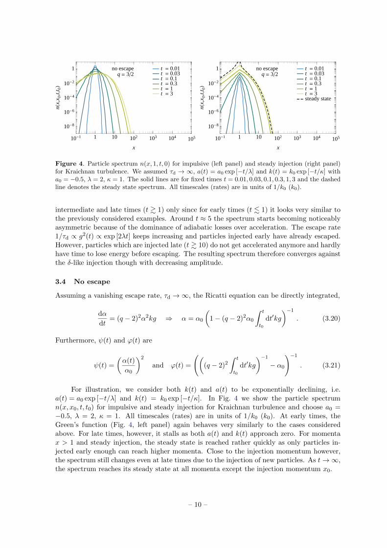
Figure 4. Particle spectrum n(x, 1, t, 0) for impulsive (left panel) and steady injection (right panel)for Kraichnan turbulence. We assumed τd → ∞, a(t) = a0 exp [−t/λ] and k(t) = k0 exp [−t/κ] witha0 = −0.5, λ = 2, κ = 1. The solid lines are for fixed times t = 0.01, 0.03, 0.1, 0.3, 1, 3 and the dashedline denotes the steady state spectrum. All timescales (rates) are in units of 1/k0 (k0).

intermediate and late times (t & 1) only since for early times (t . 1) it looks very similar tothe previously considered examples. Around t ≈ 5 the spectrum starts becoming noticeablyasymmetric because of the dominance of adiabatic losses over acceleration. The escape rate1/τd ∝ g2(t) ∝ exp [2λt] keeps increasing and particles injected early have already escaped.However, particles which are injected late (t & 10) do not get accelerated anymore and hardlyhave time to lose energy before escaping. The resulting spectrum therefore converges againstthe δ-like injection though with decreasing amplitude.

3.4 No escape

Assuming a vanishing escape rate, τd →∞, the Ricatti equation can be directly integrated,

dα

dt= (q − 2)2α2kg ⇒ α = α0

(1− (q − 2)2α0

∫ t

t0

dt′kg

)−1. (3.20)

Furthermore, ψ(t) and ϕ(t) are

ψ(t) =

(α(t)

α0

)2

and ϕ(t) =

(((q − 2)2

∫ t

t0

dt′kg

)−1− α0

)−1. (3.21)

For illustration, we consider both k(t) and a(t) to be exponentially declining, i.e.a(t) = a0 exp [−t/λ] and k(t) = k0 exp [−t/κ]. In Fig. 4 we show the particle spectrumn(x, x0, t, t0) for impulsive and steady injection for Kraichnan turbulence and choose a0 =−0.5, λ = 2, κ = 1. All timescales (rates) are in units of 1/k0 (k0). At early times, theGreen’s function (Fig. 4, left panel) again behaves very similarly to the cases consideredabove. For late times, however, it stalls as both a(t) and k(t) approach zero. For momentax > 1 and steady injection, the steady state is reached rather quickly as only particles in-jected early enough can reach higher momenta. Close to the injection momentum however,the spectrum still changes even at late times due to the injection of new particles. As t→∞,the spectrum reaches its steady state at all momenta except the injection momentum x0.

– 10 –

4 Summary and conclusion

We have presented a new solution to the Fokker-Planck equation for stochastic particleacceleration by plasma wave turbulence. In extension to previously known solutions weallow the rates for stochastic acceleration, both diffusive and convective escape as well asadiabatic losses to be time-dependent. Furthermore, we do not need to constrain ourselvesto specific values of the turbulence spectral index q and can therefore apply this result tothe phenomenologically interesting cases of Kolmogorov (q = 5/3) and Kraichnan (q =3/2) turbulence. We have investigated four examples to illustrate the qualitatively differentbehaviour of spectra due to the time-dependent rates and extended range in q. In the firstexample we constrained ourselves, however, to constant rates and neglected adiabatic lossesin order to compare our solution to previously presented results which constitutes a non-trivial test of our calculation. We have also considered the case of constant accelerationand exponentially decreasing adiabatic loss rate which leads to rather hard spectra. Incontrast, with exponentially decreasing acceleration and constant adiabatic losses, the spectrabecome very soft and no steady-state solution exists. Finally, for infinite escape time we havepresented an example with exponentially decreasing acceleration and adiabatic loss rateswhich leads to rather soft spectra in particular close to the injection energy.

A few words about boundary conditions are in order. It was pointed out [41] that theinitial value problem (IVP), eq. 2.1, with boundary conditions at x = 0 and x → ∞ issingular (see Ref. [41] for a definition and discussion of a singular IVP). Therefore, the statusof the boundary conditions is not clear but must be determined more carefully. Furthermore,the spectral theory of second order differential equations proves helpful in investigating theconditions under which a steady state solution exists. Unfortunately, it is not possible toanalyse the problem at hand in this framework, since the variable coefficients of the partialdifferential equation prevent the formulation of an equivalent boundary-value problem (BVP)of Sturm-Liouville type. However, the transformed IVP, i.e. the heat equation type eq. 2.11,must satisfy boundary conditions for f at ρ → 0,∞ similar to those that the original IVP,eq. 2.5, satisfies for f at x→ 0,∞ since both are connected by non-singular transformations.We find that ρ → 0,∞ are both limit points (for a definition see Ref. [41]) such that theappropriate boundary conditions at ρ→ 0,∞ are simply ||f || <∞ which justifies the choiceof the bounded solution in deriving eq. 2.11. Finally, we note that the discussion aboutthe existence of the steady state solution cannot be applied here either due to the variablecoefficients. As we have seen in the above examples, the existence of the steady state is largelydetermined by the time-dependence and asymptotic behaviour of the acceleration and lossrates, k(t), a(t) and τd(t) and therefore needs to be discussed on a case-by-case basis.

Acknowledgments

The author would like to thank Subir Sarkar, Brian Reville and Alex Lazarian for helpfuldiscussions and Subir Sarkar for encouragement to publish this study.

References

[1] E. Fermi, On the Origin of the Cosmic Radiation, Phys.Rev. 75 (1949) 1169–1174.

[2] C. Lacombe, Acceleration of particles and plasma heating by turbulent Alfven waves in aradiogalaxy, Astron. Astrophys. 54 (1977) 1–16.

– 11 –

[3] J. A. Eilek, Particle reacceleration in radio galaxies, Astrophys. J. 230 (1979) 373–385.

[4] A. Achterberg, The energy spectrum of electrons accelerated by weak magnetohydrodynamicturbulence, Astron. Astrophys. 76 (1979) 276–286.

[5] M. J. Hardcastle, C. C. Cheung, I. J. Feain, and L. Stawarz, High-energy particle accelerationand production of ultra-high-energy cosmic rays in the giant lobes of Centaurus A, Mont. Not.R. Astron. Soc. 393 (2009) 1041–1053, [arXiv:0808.1593].

[6] S. O’Sullivan, B. Reville, and A. Taylor, Stochastic particle acceleration in the lobes of giantradio galaxies, Mon. Not. R. Astron. Soc. 400 (2009) 248–257, [arXiv:0903.1259].

[7] A. Tramacere, E. Massaro, and A. M. Taylor, Stochastic Acceleration and the Evolution ofSpectral Distributions in SSC Sources: A Self Consistent Modeling of Blazars’ Flares,Astrophys. J. 739 (2011) 66, [arXiv:1107.1879].

[8] R. Schlickeiser, A. Sievers, and H. Thiemann, The diffuse radio emission from the Comacluster, Astron. Astrophys. 182 (1987) 21–35.

[9] V. Petrosian, On the Nonthermal Emission and Acceleration of Electrons in Coma and OtherClusters of Galaxies, Astrophys. J. 557 (2001) 560–572, [astro-ph/0101145].

[10] G. Brunetti, P. Blasi, R. Cassano, and S. Gabici, Alfvenic reacceleration of relativistic particlesin galaxy clusters: MHD waves, leptons and hadrons, Mon. Not. R. Astron. Soc. 350 (2004)1174, [astro-ph/0312482].

[11] G. Brunetti and A. Lazarian, Compressible Turbulence in Galaxy Clusters: Physics andStochastic Particle Re-acceleration, Mon. Not. R. Astron. Soc. 378 (2007) 245–275,[astro-ph/0703591].

[12] E. Waxman, Cosmological gamma-ray bursts and the highest energy cosmic rays, Phys. Rev.Lett. 75 (1995) 386–389, [astro-ph/9505082].

[13] C. D. Dermer and M. Humi, Adiabatic losses and ultra-high energy cosmic ray acceleration ingamma ray burst blast waves, Astrophys. J. 556 (2001) 479–493, [astro-ph/0012272].

[14] L. Stawarz and M. Ostrowski, Radiation from the Relativistic Jet: a Role of the ShearBoundary Layer, Astrophys. J. 578 (2002) 763–774, [astro-ph/0203040].

[15] L. Stawarz, M. Sikora, M. Ostrowski, and M. C. Begelman, On Multiwavelength Emission ofLarge-Scale Quasar Jets, Astrophys. J. 608 (2004) 95–107, [astro-ph/0401356].

[16] K. Katarzynski, G. Ghisellini, A. Mastichiadis, F. Tavecchio, and L. Maraschi, Stochasticparticle acceleration and synchrotron self-Compton radiation in TeV blazars, Astron.Astrophys. 453 (2006) 47–56, [astro-ph/0603362].

[17] B. Giebels, G. Dubus, and B. Khelifi, Unveiling the X-ray/TeV engine in Mkn 421,Astron.Astrophys. 462 (2007) 29–41, [astro-ph/0610270].

[18] V. Petrosian and T. Q. Donaghy, On the Spatial Distribution of Hard X-Rays from Solar FlareLoops, Astrophys. J. 527 (1999) 945–957, [astro-ph/9907181].

[19] S.-M. Liu, V. Petrosian, and G. M. Mason, Stochastic Acceleration of 3He and 4He by ParallelPropagating Plasma Waves, Astrophys. J. 613 (2004) L81, [astro-ph/0403007].

[20] V. Petrosian and S.-M. Liu, Stochastic Acceleration of Electrons and Protons. I. Accelerationby Parallel Propagating Waves, Astrophys. J. 610 (2004) 550–571, [astro-ph/0401585].

[21] M. Simon, W. Heinrich, and K. D. Mathis, Propagation of injected cosmic rays underdistributed reacceleration, Astrophys. J. 300 (1986) 32–40.

[22] E. S. Seo and V. S. Ptuskin, Stochastic reacceleration of cosmic rays in the interstellar medium,Astrophys. J. 431 (1994) 705–714.

[23] S.-M. Liu, V. Petrosian, and F. Melia, Electron Acceleration around the Supermassive Black

– 12 –

Hole at the Galactic Center, Astrophys. J. 611 (2004) L101–L104, [astro-ph/0403487].

[24] A. Atoyan and C. D. Dermer, TeV emission from the Galactic Center black-hole plerion,Astrophys.J. 617 (2004) L123–L126, [astro-ph/0410243].

[25] J. S. Scott and R. A. Chevalier, Cosmic-ray production in the Cassiopeia A supernovaremnant, Astrophys. J. Lett. 197 (1975) L5–L8.

[26] R. Cowsik and S. Sarkar, The evolution of supernova remnants as radio sources, Mon. Not. R.Astron. Soc. 207 (1984) 745.

[27] Z. Fan, S. Liu, and C. L. Fryer, Stochastic Electron Acceleration in the TeV SupernovaRemnant RX J1713.7-3946: The High-Energy Cut-off, Mon. Not. R. Astron. Soc. 406 (2009)1337–1349, [arXiv:0909.3349].

[28] P. Mertsch and S. Sarkar, Fermi gamma-ray ‘bubbles’ from stochastic acceleration of electrons,Phys.Rev.Lett. 107 (2011) 091101, [arXiv:1104.3585].

[29] R. Schlickeiser, Cosmic ray astrophysics. Springer, Berlin, 2002.

[30] D. B. Melrose, The Emission and Absorption of Waves by Charged Particles in MagnetizedPlasmas, Ap&SS 2 (1968) 171–235.

[31] R. Kulsrud and W. P. Pearce, The Effect of Wave-Particle Interactions on the Propagation ofCosmic Rays, Astrophys. J. 156 (1969) 445.

[32] R. Schlickeiser, Cosmic-ray transport and acceleration. I - Derivation of the kinetic equationand application to cosmic rays in static cold media., Astrophys. J. 336 (1989) 243–293.

[33] Y. Zhou and W. H. Matthaeus, Models of inertial range spectra of interplanetarymagnetohydrodynamic turbulence, J. Geophys. Res. 95 (1990) 14881–14892.

[34] R. Dung and R. Schlickeiser, The influence of the Alfvenic cross and magnetic helicity on thecosmic ray transport equation. I - Isospectral slab turbulence, Astron. Astrophys. 240 (1990)537–540.

[35] P. Goldreich and S. Sridhar, Toward a theory of interstellar turbulence. 2: Strong alfvenicturbulence, Astrophys. J. 438 (1995) 763–775.

[36] J. Cho and A. Lazarian, Compressible sub-alfvenic MHD turbulence in low-Beta plasmas, Phys.Rev. Lett. 88 (2002) 245001, [astro-ph/0205282].

[37] R. Schlickeiser and J. A. Miller, Quasi-linear Theory of Cosmic-Ray Transport andAcceleration: The Role of Oblique Magnetohydrodynamic Waves and Transit-Time Damping,Astrophys. J. 492 (1998) 352.

[38] J. Cho and A. Lazarian, Particle acceleration by MHD turbulence, Astrophys. J. 638 (2006)811–826, [astro-ph/0509385].

[39] S. A. Kaplan, The Theory of the Acceleration of Charged Particles by Isotopic Gas MagneticTurbulent Fields, J. Exper. Theoret. Phys. 2 (1956) 203–210.

[40] N. S. Kardashev, Nonstationarity of Spectra of Young Sources of Nonthermal Radio Emission,Soviet Ast. 6 (1962) 317–327.

[41] B. T. Park and V. Petrosian, Fokker-Planck Equations of Stochastic Acceleration: Green’sFunctions and Boundary Conditions, Astrophys. J. 446 (1995) 699–716.

[42] P. Becker, T. Le, and C. D. Dermer, Time-Dependent Stochastic Particle Acceleration inAstrophysical Plasmas: Exact Solutions Including Momentum-Dependent Escape, Astrophys.J.647 (2006) 539–551, [astro-ph/0604504].

[43] Y. Fedorov and M. Stehlik, Stochastic acceleration by the induced electric field versus the Fermiacceleration, Journal of Physics B Atomic Molecular Physics 43 (2010) 185701.

– 13 –

[44] S. F. Gull, A numerical model of the structure and evolution of young supernova remnants,Mont. Not. R. Astron. Soc. 161 (1973) 47–69.

[45] J. Tammi and P. Duffy, Particle-acceleration timescales in TeV blazar flares, AIP Conf. Proc.1085 (2009) 475–478, [arXiv:0811.3573].

[46] R. Schlickeiser, Cosmic-Ray Transport and Acceleration. II. Cosmic Rays in Moving ColdMedia with Application to Diffusive Shock Wave Acceleration, Astrophys. J. 336 (1989) 264.

[47] G. M. Murphy, Ordinary Differential Equations and Their Solutions. D. Van Nostrand, NewYork, 1960.

[48] E. Kamke, Differentialgleichungen: Losungsmethoden und Losungen, I, GewohnlicheDifferentialgleichungen. B. G. Teubner, Leipzig, 1977.

[49] A. D. Polyanin and V. F. Zaitsev, Handbook of Exact Solutions for Ordinary DifferentialEquations. CRC Press, Boca Raton, 1995.

– 14 –