a multi-objective linear programming model for ranking
TRANSCRIPT
Aalto University
School of Science
Master’s Programme in Mathematics and Operations Research
Visa Linkio
A Multi-Objective Linear Programming Modelfor Ranking Competing Refineries
Master’s Thesis
Espoo, May 27, 2018
Supervisor: Professor Kai Virtanen, Aalto University
Advisor: M.Sc. (Tech.) Esa Svahn, Neste
The document can be stored and made available to the public on the open Internet pages of
Aalto University. All other rights are reserved.

Aalto University
School of Science
Master’s Programme in Mathematics and Operations Re-
search
ABSTRACT OF
MASTER’S THESIS
Author: Visa Linkio
Title:
A Multi-Objective Linear Programming Model for Ranking Competing Refineries
Date: May 27, 2018 Pages: vii + 67
Major: Systems and Operations Research Code: SCI3055
Supervisor: Professor Kai Virtanen, Aalto University
Advisor: M.Sc. (Tech.) Esa Svahn, Neste
For benchmarking, a petroleum refining company is interested in how different
market scenarios affect their competitors. This thesis is a feasibility study for the
use of a multi-objective linear programming (MOLP) model for analyzing the
impact of market prices on competing petroleum refineries.
Linear programming (LP) models are widely used for optimizing petroleum refin-
ery operation. The existing LP models can be utilized in the design of a MOLP
model which makes it a particuarly desired model type. MOLP is a method for
solving linear problems where multiple conflicting objective functions are opti-
mized simultaneously. In this case, the different objective functions depict the
profits of competing companies. Since there are several decision makers, this
problem is different from those that have been extensively studied in open liter-
ature.
In this thesis, a MOLP model labeled the Refinery Ranking Model (RRM) is de-
signed. The user sets the market parameters for the RRM which then determines
the optimal purchases and sales for each refining company.
The results indicate that MOLP can be used to analyze the market dynamics of
competing refining companies. The RRM could be expanded to include dozens of
refineries and still describe their detailed behavior well and with a very reasonable
solution time.
Keywords: Competition, Linear programming, Multi-objective linear
programming, Network optimization, Petroleum refining,
Supply chain planning
Language: English
ii

Aalto-yliopisto
Perustieteiden korkeakoulu
Matematiikan ja operaatiotutkimuksen maisteriohjelma
DIPLOMITYON
TIIVISTELMA
Tekija: Visa Linkio
Tyon nimi:
Lineaarinen monitavoiteoptimointimalli kilpailevien jalostamoiden vertailuun
Paivays: 27. toukokuuta 2018 Sivumaara: vii + 67
Paaaine: Systeemi- ja operaatiotutkimus Koodi: SCI3055
Valvoja: Professori Kai Virtanen, Aalto-yliopisto
Ohjaaja: Diplomi-insinoori Esa Svahn, Neste
Oljynjalostajille, kuten muillekin yrityksille, on hyodyllista verrata omaa toimin-
taansa kilpailijoihinsa. Tama diplomityo on soveltuvuustutkimus, joka selvittaa
lineaarisen monitavoiteoptimoinnin (MOLP) soveltuvuutta mallintamaan mark-
kinatilanteiden vaikutuksia kilpaileviin oljynjalostamoihin.
Lineaarista ohjelmointia kaytetaan laajalti oljynjalostamoiden toiminnan opti-
mointiin. Koska oljynjalostajilla on osaamista tallaisista malleista, MOLP-mallin
rakentaminen on verrattain helppoa. MOLP on menetelma, jolla ratkaistaan li-
neaarisia ongelmia, joissa yritetaan minimoida tai maksimoida useita keskenaan
ristiriitaisia tavoiteyhtaloita. Taman tyon tapauksessa nama tavoiteyhtalot ovat
kilpailevien oljynjalostajien tulokset. Koska kukin jalostaja pyrkii optimoimaan
omaa tulostaan muista valittamatta, on ongelmassa useita paatoksentekijoita.
Tama erottaa kyseisen tapauksen aiemmin julkisessa kirjallisuudessa kasitellyista
MOLP-malleista.
Tassa tyossa luodaan kilpailevien jalostamoiden toimintaa ja tuottavuutta ku-
vaava MOLP-malli. Kayttaja voi syottaa malliin markkinahintoja ja muita para-
metreja. Tyon tulokset osoittavat, etta MOLP-mallia voidaan kayttaa tallaiseen
analyysiin. Mallia voitaisiin myos laajentaa kattamaan kymmenia jalostamoita
ilman, etta tarkkuus tai ratkaisuaika karsisivat suuresti.
Asiasanat: Kilpailu, Lineaarinen monitavoiteoptimointi, Lineaarinen oh-
jelmointi, Toimitusketjun suunnittelu, Verkko-optimointi,
Oljynjalostus
Kieli: Englanti
iii
Acknowledgements
I would like to thank the people at Neste who expressed their interest in this thesis
and provided a vast repertory of information. Especial praise belongs to Esa Svahn
and Jonna Falck for offering this interesting topic and for always finding the time
to support the creation of this work. I also express my gratitude to my supervis-
ing professor Kai Virtanen for extremely valuable advice when it would have been
otherwise unclear how to proceed. Esa and Kai also agreed to review and evalu-
ate this thesis on a tight schedule for which I am grateful. Commendation also to
Otto Puomio for voluntarily providing detailed feedback and many suggestions for
improving this thesis. Additionally, I wish to thank my family and friends for their
continued support and care.
Espoo, May 27, 2018
Visa Linkio
iv
Abbreviations and Acronyms
bbl Barrel
bbl/d Barrels per day
CCU Catalytic Cracking Unit
CDU Crude Distillation Unit
FOB Free On Board
kbbl 1000 barrels
kbbl/d 1000 barrels per day
LP Linear Programming
LPG Liquified Petroleum Gas
MOLP Multi-Objective Linear Programming
MOO Multi-Objective Optimization
RRM Refinery Ranking Model
SCP Supply Chain Planning
VDU Vacuum Distillation Unit
VGO Vacuum Gas Oil
v
Contents
Abstract . . . . . . . . . . . . . . . . . . . . . . . . . . . . . . . . . . . . . ii
Abstract (in Finnish) . . . . . . . . . . . . . . . . . . . . . . . . . . . . . . iii
Acknowledgements . . . . . . . . . . . . . . . . . . . . . . . . . . . . . . . iv
Abbreviations and Acronyms . . . . . . . . . . . . . . . . . . . . . . . . . v
1 Introduction 1
2 Overview of Alternative Methods 4
3 Petroleum Refining 9
3.1 Petroleum Products . . . . . . . . . . . . . . . . . . . . . . . . . . . . 9
3.2 Crude Oil . . . . . . . . . . . . . . . . . . . . . . . . . . . . . . . . . 12
3.3 Refinery Configuration . . . . . . . . . . . . . . . . . . . . . . . . . . 12
3.4 Refining Margin . . . . . . . . . . . . . . . . . . . . . . . . . . . . . . 17
3.5 Supply Chain Planning . . . . . . . . . . . . . . . . . . . . . . . . . . 19
3.6 Petroleum Refining in the Refinery Ranking Model . . . . . . . . . . 21
4 Optimization Methods 22
4.1 Multi-Objective Optimization . . . . . . . . . . . . . . . . . . . . . . 22
4.2 Multi-Objective Linear Programming . . . . . . . . . . . . . . . . . . 24
4.3 Selection of Multi-Objective Linear Programming Methods . . . . . . 26
5 The Refinery Ranking Model 30
5.1 General structure . . . . . . . . . . . . . . . . . . . . . . . . . . . . . 31
5.2 Notation . . . . . . . . . . . . . . . . . . . . . . . . . . . . . . . . . . 33
5.3 Assumptions . . . . . . . . . . . . . . . . . . . . . . . . . . . . . . . . 35
5.4 Decision Variables . . . . . . . . . . . . . . . . . . . . . . . . . . . . . 36
5.5 Objective Functions . . . . . . . . . . . . . . . . . . . . . . . . . . . . 36
5.6 Constraints . . . . . . . . . . . . . . . . . . . . . . . . . . . . . . . . 37
6 Validation of the Refinery Ranking Model 39
6.1 Validation of the Refinery Linear Programming Models . . . . . . . . 39
vi
6.2 Validation of the Multi-Objective Linear Programming Model . . . . 45
6.3 Robustness and Solution Time . . . . . . . . . . . . . . . . . . . . . . 48
7 Market Price Sensitivity of Refining Margins 53
8 Discussion 57
8.1 Avoiding Undesired Behavior in the Refinery Ranking Model . . . . . 58
8.2 Model Complexity . . . . . . . . . . . . . . . . . . . . . . . . . . . . 58
8.3 Price Parameters and Game Theory . . . . . . . . . . . . . . . . . . . 60
9 Conclusions 62
Bibliography 65
vii
Chapter 1
Introduction
Linear programming (LP) is a method of mathematical optimization. It has been
used extensively in industry solutions in oil refining among other fields. Academic
articles, such as Symonds [1955], describing LP solutions for oil refining problems
date back to the 1950s. Other articles, including Bana e Costa [1990], describe the
use of Multi-Objective Linear Programming (MOLP) in oil refining. In MOLP, there
are several conflicting objectives to be optimized and a good compromise solution is
sought for [Sakawa et al., 2013]. However, to this day the public articles concerning
the refining industry concentrate on problems where the LP or MOLP problem only
covers the perspective a single decision maker. These include the optimization of
blending components into final products with several attributes to be optimized
[Bana e Costa, 1990]. This is similar to the optimization of the operation of a
refinery or a group of refineries working towards a mutual goal. Thus, there is a
void of research about using MOLP to describe systems of several decision makers
with conflicting goals. This thesis aims to create a MOLP model that can be used
to rank several competing refining companies in different market situations. In
such circumstances, the conflicts between different objective functions are highly
fascinating. No refining company is willing to give up their own good for the others.
Therefore, the model solution must be a carefully selected compromise to achieve
realism.
This thesis is commissioned by a Finnish oil refining and renewable solutions com-
pany Neste. They request a feasibility study on a mathematical model that could
be used to compare the profitability of competing oil refineries. The model should
be created on the Spiral Suite1 optimization software. The models in the software
are formulated as LP models. This naturally leads to the conclusion that the model
designed in this thesis needs to be a MOLP model since the goals of different refining
1 Spiral Suite by AVEVATM
CHAPTER 1. INTRODUCTION 2
companies must be considered. The model is labeled the Refinery Ranking Model
(RRM).
Neste has a strong presence in the Baltic countries and the St. Petersburg region
and they aim to become the leading supplier of fuel solutions in the Baltic Sea
region. The company produces renewable products in Finland, the Netherlands,
and Singapore as well as crude oil-based products in Finland. In addition they are
co-owners of a base oil plant in Bahrain. From now on, Neste shall be referred to as
the case company. [Neste, 2017]
The RRM calculates the sales, purchases, and profitability of the competing re-
fineries in market situations given by the user. A prototype RRM containing five
European refineries is built and tested as a part of this thesis in order to assess the
accuracy and practicality of such a model.
It is worth noting that although the RRM is formulated as a linear programming
model, there are some non-linearities included. These non-linearities have to do with
how the software handles some of the properties of hydrocarbon streams. Naturally
many chemical and physical processes at a petroleum refinery are nonlinear by na-
ture. Therefore, even though the problem is formulated as a MOLP problem, the
final formulation in the software is a non-linear multi-objective optimization (MOO)
problem. This thesis does not delve into these non-linearities other than analyzing
whether the non-linear behavior seen in the model results is within acceptable limits.
Because of the non-linearities, the model can also converge into local optima. Such
a behavior can be avoided to some degree by using several starting points for the
solution algorithm.
Since the objective functions of different companies conflict, there is no single correct
solution to the problem. Instead, there are several potential solutions from which one
must be selected based on a chosen selection method. The selection method must
describe the self-interest of each competing company in order to provide accurate
results. The accuracy of the RRM can be tested by market scenarios for which the
correct results can be reliably concluded based on prior knowledge. This knowledge
can be from some combination of historical data, economical theories, or factors
related to process technology at the refineries.
This thesis is structured as follows. Chapter 2 introduces related existing work and
covers some alternative approaches to the problem. Chapter 3 introduces some of
the basic concepts of refining crude oil into petroleum products. This provides the
reader with an understanding of the processes implemented in the RRM. Chapter
4 delves into the methodology of multi-objective optimization. Chapter 5 describes
CHAPTER 1. INTRODUCTION 3
how these methods are used to implement the RRM. The RRM is then validated in
Chapter 6, and Chapter 7 explores the model’s sensitivity to variations in market
prices. Chapter 8 discusses the challenges in the future development of the model.
Finally, Chapter 9 summarizes the thesis.
Chapter 2
Overview of Alternative Methods
Much of the existing work on practical MOLP problems deals with situations where
all of the objective functions, even though mutually conflicting, depict benefit for
a single decision maker. Bana e Costa [1990] gave a relevant example situation
where an oil refinery would try to simultaneously minimize cost, crude imports, high
sulfur crude, and deviations from demand state. In such a situation, the refinery is
a single agent looking for a Pareto-optimal solution and it can choose any feasible
solution according to its preferences. In the scope of this thesis, there exists several
companies each of which aims to maximize their own objective function. Therefore,
there is no single decision maker capable of selecting a preferred solution out of some
Pareto-optimal candidates. Several different approaches could be used to model the
dynamics of competing refining companies. This chapter delves into some of these
approaches and analyzes whether they could be efficient choices given the data
available.
The analyzed system is a subset of all the refineries in the world. Depending on the
scale of interest, this subset could easily contain dozens of interconnected refineries.
Due to the large scale and somewhat chaotic nature of such large systems, big
data methods could provide good results if the required data is available. However,
there is only limited reference data available for model design and validation. It
is challenging to maintain detailed up-to-date data of the sales, purchases, and
technical details of dozens of refineries. Therefore, the data is likely to be incomplete,
disjointed, and partially outdated. Thus, methods that require large amounts of data
are likely infeasible. In addition to big data methods, this applies to many methods
featuring time series analysis or stochasticity. If even some aspects of each refinery,
e.g. only their sales, could be obtained on a frequent basis, solutions that partially
utilize these types of models could be considered.
4

CHAPTER 2. OVERVIEW OF ALTERNATIVE METHODS 5
Despite the absence of proper time series in the reference data, dynamic models are
not entirely ruled out. A model can be constructed based on a data set that depicts
a static moment in time. Combined with theoretical knowledge about refinery tech-
nology and petroleum markets, the technical and trade details of each refinery are
used to model how refinery input, output, and profitability depend on the market.
Then, market parameters are given and the model provides a solution. The solution
can be used as a starting point for a new solution. Therefore, a time series of market
parameters can be chosen and a time series of trades and profits can be obtained
as a solution. In this way, static data can be used to study dynamic scenarios. In
practice, this can be achieved with a MOLP model if multiple successive runs are
made.
Another approach is to form a state-space model. A state-space representation
depicts a system as a set of input, output, and state variables which are related to
each other by first order difference or differential equations [Friedland, 1986]. An nth
order differential equation can be replaced by a state-space representation containing
only first order difference or differential equations [Friedland, 1986]. A state-space
model is in essence a time series model in which one or several unobserved time series
are used to describe an observed time series [Leeflang et al., 2017]. The unobserved
time series are called the states of the model [Leeflang et al., 2017]. The initial
values of the time series can be defined by the user based on the desired scenario.
For instance, a time series of market prices could be given as an input and their
effects on the refineries’ profitability could be observed. In this example, the market
price time series is simply a scenario and thus no existing data is required. To discuss
the feasibility of a state-space model for a system of competing refineries, consider
the following discrete-time state-space representation of a nonlinear system
x(t) = A(t)x(t) + B(t)u(t) (2.1)
y(t) = x(t)u(t) (2.2)
where
x(t) is a state vector containing the current sales and purchases, x(t) ∈ Rn
y(t) is the output vector containing the refining margins of each refinery, y(t) ∈ Rq
u(t) is the input vector containing the current market prices, u(t) ∈ Rp
A(t) is the state matrix
B(t) is the input matrix
x(t) :=d
dtx(t) is the time derivative of x(t)
CHAPTER 2. OVERVIEW OF ALTERNATIVE METHODS 6
In this case, the states are the sales and purchases of the competing refineries.
Consider Equation 2.1. The system matrix A(t) describes how the current states
affect future states. High current state should lead to low future state. For example,
a high amount of gasoline sales could mean that the inventories of the customers
are filled and the demand will be lower in the next time period. The input matrix
B(t) describes how the current input u(t) affects the future states. In this case, the
input vector would be a vector of market prices. Thus, higher input values would
lead to an increase in x(t) for those elements of u(t) that correspond to products
saleable from the refineries and decrease in x(t) for those that correspond to goods
that the refineries purchase.
Now, consider Equation 2.2. The output y(t) is a vector of profits earned by each
refinery in the model. The profit of a refinery equals the units of goods traded
multiplied by the price per unit of those goods.
Forming a state-space model requires either quality data or strong understanding
of the analyzed system. For a system of competing refining companies that goes
to such detail as in this thesis, this is a challenging task. The competitive aspect
requires careful consideration. Leeflang [2008] and Leeflang et al. [2017] discuss how
competition models have developed. They state that the first models found the
optimal solution for only a single company at a time. They continue to explain
that eventually game theoretic models were developed. In game theoretic competi-
tion models multiple players maximize their utilities simultaneously [Leeflang et al.,
2017]. The competition between several refining companies certainly has a strong
game theoretic aspect to it. Each company aims to maximize their own profit but
are affected by the simultaneous actions of their competitors. For example, the
trade deals one company can make are affected by deals of other companies because
regional supplies and demands are limited.
Fernandez et al. [2005] discuss competition and cooperation in linear production
games. These are games where each player faces a linear production problem. Specif-
ically, Fernandez et al. [2005] consider a game where all the players produce the same
goods but with different linear technologies and prices. Three analyses of this game
are presented. The first one is a non-cooperative analysis and the other two are
different cooperative analyses. One of the cooperative analyses features transferable
utility and the other one does not. Transferable utility refers to a situation where
the total utility of all players can be allocated freely among the players as opposed
to being strictly a result of the production of the respective player. [Fernandez et al.,
2005]
The system of competing refineries can be described as a game where the players

CHAPTER 2. OVERVIEW OF ALTERNATIVE METHODS 7
produce identical goods but with different prices and different technologies. The
goods sold by each refinery need to be classified under some predetermined stan-
dard products regardless of the type of model used. This is to avoid unnecessary
complexity. However, product prices need to differ from refinery to refinery since
the transportation costs differ based on geographical location. Similarly, the tech-
nologies unique to each refinery depict the respective refinery’s capability to turn
certain raw materials into certain products.
Naturally, the competition between refining companies is non-cooperative. However,
some refining companies own several refineries and there is not only cooperation but
also transferable utility between refineries belonging to the same company. There-
fore, should the system be described as a linear production game there is a question
of how to depict refining companies that own several refineries. One method is to
abstract each refining company to only have a single refinery that has the attributes
of all the refineries of that company combined. This would be a simple way to man-
age the cooperation and transferable utility that are present only within refining
companies and not between them. The downside is a loss of detail e.g. concerning
transportation costs.
In a cooperative game, the optimal solutions are in the core of the game [Barron,
2013]. The core is the set of feasible allocations where the players receive at least
as much utility as they would if they did not cooperate [Barron, 2013]. It has been
shown that for large cooperative production games the core of the game is non-empty
under certain assumptions [Flam et al., 1975]. This suggests that if the problem
involves a large enough number of companies then there exists a cooperative solution
to the problem such that the companies can not improve their profit. Although such
a solution assumes cooperation, it could contribute to the use of a non-cooperative
game theoretic model or any other type of model. It could be used to explore the
optimal solutions, thus providing insight to the quality of the results of another
model. For example, convergence to local optimum could be suspected based on
comparison to the cooperative game theoretic model.
In conclusion, the Refinery Ranking Model should be implemented as a MOLP
model since the case company has existing LP models which can be used as guide-
lines for the design. Attempting to construct a large-scale state-space model or a
complicated game theoretic model is not the key competency of the case company.
However, if the MOLP model is found to be inadequate, it is possible to consider
these alternative models in the future. Other potential model types may exist, and
the system can potentially be split into sub-problems which are solved using differ-
ent types of models. On a certain level of abstraction, the production problem and

CHAPTER 2. OVERVIEW OF ALTERNATIVE METHODS 8
the transportation problem of a refinery can be seen as separate problems although
in reality they affect each other.
Chapter 3
Petroleum Refining
This chapter explains how crude oil is turned into petroleum products in a petroleum
refinery. The petroleum supply chain is introduced in Figure 3.1. The petroleum
market, refinery configuration, and the process units at the refinery are explained to
help the reader understand the mathematical model described in Chapter 5.
A note should be made on terminology to avoid confusion. This thesis discusses
raw materials and end products of petroleum refining. It also discusses the markets
where both of these are sold and the refineries that turn raw materials into end
products. Sometimes goods can be sold from one refinery as products to another
refinery which processes them further and sells as more valuable products. There-
fore, the difference between raw materials and end products can be vague. In this
thesis, the term ‘goods’ refers to all materials that are either purchased, sold, or
both. The term ‘product’ refers to all goods that a refinery sells. Most of these are
‘end products’ that are sold to the market while some are ‘intermediate products’
sold to other refineries for further processing. All the purchases that refineries make
are collectively labeled ‘raw materials’. Thus, an intermediate product belongs in
both products and raw materials.
3.1 Petroleum Products
In order to understand the petroleum market, the mutual relationships of different
petroleum products are explained briefly. Petroleum is a mixture composed mainly
of hydrocarbons and is found in sedimentary rocks. A hydrocarbon is a compound
that contains only hydrogen (H) and carbon (C). Petroleum occurs as gas, liquid,
9
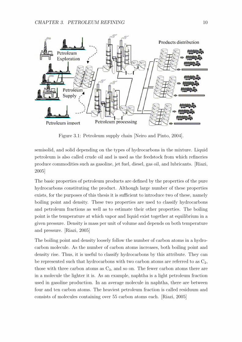
CHAPTER 3. PETROLEUM REFINING 10
Figure 3.1: Petroleum supply chain [Neiro and Pinto, 2004].
semisolid, and solid depending on the types of hydrocarbons in the mixture. Liquid
petroleum is also called crude oil and is used as the feedstock from which refineries
produce commodities such as gasoline, jet fuel, diesel, gas oil, and lubricants. [Riazi,
2005]
The basic properties of petroleum products are defined by the properties of the pure
hydrocarbons constituting the product. Although large number of these properties
exists, for the purposes of this thesis it is sufficient to introduce two of these, namely
boiling point and density. These two properties are used to classify hydrocarbons
and petroleum fractions as well as to estimate their other properties. The boiling
point is the temperature at which vapor and liquid exist together at equilibrium in a
given pressure. Density is mass per unit of volume and depends on both temperature
and pressure. [Riazi, 2005]
The boiling point and density loosely follow the number of carbon atoms in a hydro-
carbon molecule. As the number of carbon atoms increases, both boiling point and
density rise. Thus, it is useful to classify hydrocarbons by this attribute. They can
be represented such that hydrocarbons with two carbon atoms are referred to as C2,
those with three carbon atoms as C3, and so on. The fewer carbon atoms there are
in a molecule the lighter it is. As an example, naphtha is a light petroleum fraction
used in gasoline production. In an average molecule in naphtha, there are between
four and ten carbon atoms. The heaviest petroleum fraction is called residuum and
consists of molecules containing over 55 carbon atoms each. [Riazi, 2005]
CHAPTER 3. PETROLEUM REFINING 11
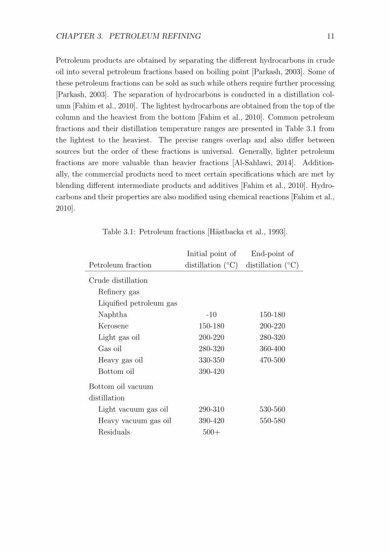
Petroleum products are obtained by separating the different hydrocarbons in crude
oil into several petroleum fractions based on boiling point [Parkash, 2003]. Some of
these petroleum fractions can be sold as such while others require further processing
[Parkash, 2003]. The separation of hydrocarbons is conducted in a distillation col-
umn [Fahim et al., 2010]. The lightest hydrocarbons are obtained from the top of the
column and the heaviest from the bottom [Fahim et al., 2010]. Common petroleum
fractions and their distillation temperature ranges are presented in Table 3.1 from
the lightest to the heaviest. The precise ranges overlap and also differ between
sources but the order of these fractions is universal. Generally, lighter petroleum
fractions are more valuable than heavier fractions [Al-Sahlawi, 2014]. Addition-
ally, the commercial products need to meet certain specifications which are met by
blending different intermediate products and additives [Fahim et al., 2010]. Hydro-
carbons and their properties are also modified using chemical reactions [Fahim et al.,
2010].
Table 3.1: Petroleum fractions [Hastbacka et al., 1993].
Initial point of End-point of
Petroleum fraction distillation (◦C) distillation (◦C)
Crude distillation
Refinery gas
Liquified petroleum gas
Naphtha -10 150-180
Kerosene 150-180 200-220
Light gas oil 200-220 280-320
Gas oil 280-320 360-400
Heavy gas oil 330-350 470-500
Bottom oil 390-420
Bottom oil vacuum
distillation
Light vacuum gas oil 290-310 530-560
Heavy vacuum gas oil 390-420 550-580
Residuals 500+
CHAPTER 3. PETROLEUM REFINING 12
3.2 Crude Oil
Crude oils from different regions have different characteristics. The two most impor-
tant characteristics are sulfur content and density, the latter of which is an indicator
of the crude oil’s hydrocarbon mixture [Speight, 2011]. Low-density crude oils are
described as ‘light’ and those with high density as ‘heavy’ [Speight, 2011]. Simi-
larly, crude oils with low sulfur content are described as ‘sweet’ and those with high
sulfur content as ‘sour’ [Speight, 2011]. The number of different crude oil types
amount probably over 400 [Bret-Rouzaut and Favennec, 2011]. When crude oils
are processed at a refinery, they yield different products as described briefly in Sec-
tion 3.1. The type of a crude oil used determines the ratio of different petroleum
fractions whereas refinery configuration affects the ratio of different end products
[Fahim et al., 2010]. More complex refinery configurations enable creating a higher
fraction of valuable products [Fahim et al., 2010].
Generally, crude oils that are lighter and have a lower sulfur content are more valu-
able. Lighter crude oil has a higher share of more valuable hydrocarbons whereas
low sulfur content is beneficial since the maximum sulfur content in end products is
regulated by law and sulfur removal is costly. Naturally, the locations of the crude
oil provider and the refinery customer determine the transportation costs and there-
fore affect the value of different crude oils to different refineries. [Bret-Rouzaut and
Favennec, 2011]
Due to high fixed costs, crude oil production responds slowly to changes in price.
The short-run supply elasticity with respect to price is considered to be 0.02 meaning
that the change in production is only 2% of the change in price. Also, the demand for
final petroleum products is inelastic with respect to price. [Al-Sahlawi, 2014]
3.3 Refinery Configuration
After crude oil is distilled into petroleum fractions, their chemical structure is modi-
fied in chemical reactions such as reforming, cracking, and desulfurization [Hastbacka
et al., 1993]. Distillation units and reactor units together are referred to as process
units. The Refinery Ranking Model (RRM) presented in Chapter 5 contains several
different process units. A selected few are listed in Table 3.2 and used later in this
section to describe refinery complexity.
CHAPTER 3. PETROLEUM REFINING 13
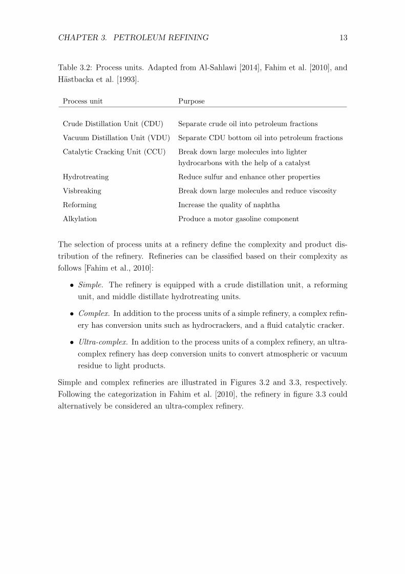
Table 3.2: Process units. Adapted from Al-Sahlawi [2014], Fahim et al. [2010], and
Hastbacka et al. [1993].
Process unit Purpose
Crude Distillation Unit (CDU) Separate crude oil into petroleum fractions
Vacuum Distillation Unit (VDU) Separate CDU bottom oil into petroleum fractions
Catalytic Cracking Unit (CCU) Break down large molecules into lighter
hydrocarbons with the help of a catalyst
Hydrotreating Reduce sulfur and enhance other properties
Visbreaking Break down large molecules and reduce viscosity
Reforming Increase the quality of naphtha
Alkylation Produce a motor gasoline component
The selection of process units at a refinery define the complexity and product dis-
tribution of the refinery. Refineries can be classified based on their complexity as
follows [Fahim et al., 2010]:
• Simple. The refinery is equipped with a crude distillation unit, a reforming
unit, and middle distillate hydrotreating units.
• Complex. In addition to the process units of a simple refinery, a complex refin-
ery has conversion units such as hydrocrackers, and a fluid catalytic cracker.
• Ultra-complex. In addition to the process units of a complex refinery, an ultra-
complex refinery has deep conversion units to convert atmospheric or vacuum
residue to light products.
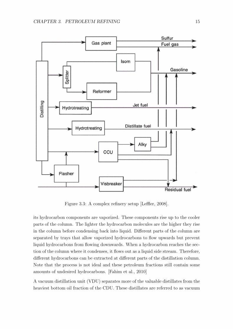
Simple and complex refineries are illustrated in Figures 3.2 and 3.3, respectively.
Following the categorization in Fahim et al. [2010], the refinery in figure 3.3 could
alternatively be considered an ultra-complex refinery.
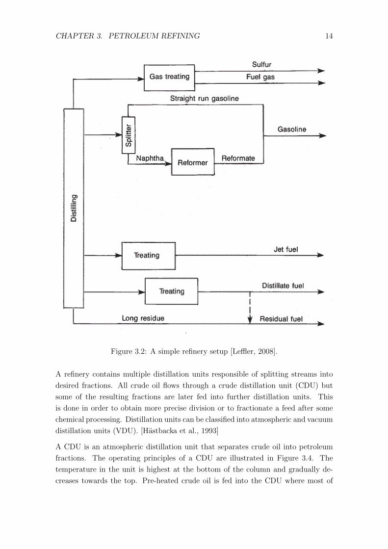
CHAPTER 3. PETROLEUM REFINING 14
Figure 3.2: A simple refinery setup [Leffler, 2008].
A refinery contains multiple distillation units responsible of splitting streams into
desired fractions. All crude oil flows through a crude distillation unit (CDU) but
some of the resulting fractions are later fed into further distillation units. This
is done in order to obtain more precise division or to fractionate a feed after some
chemical processing. Distillation units can be classified into atmospheric and vacuum
distillation units (VDU). [Hastbacka et al., 1993]
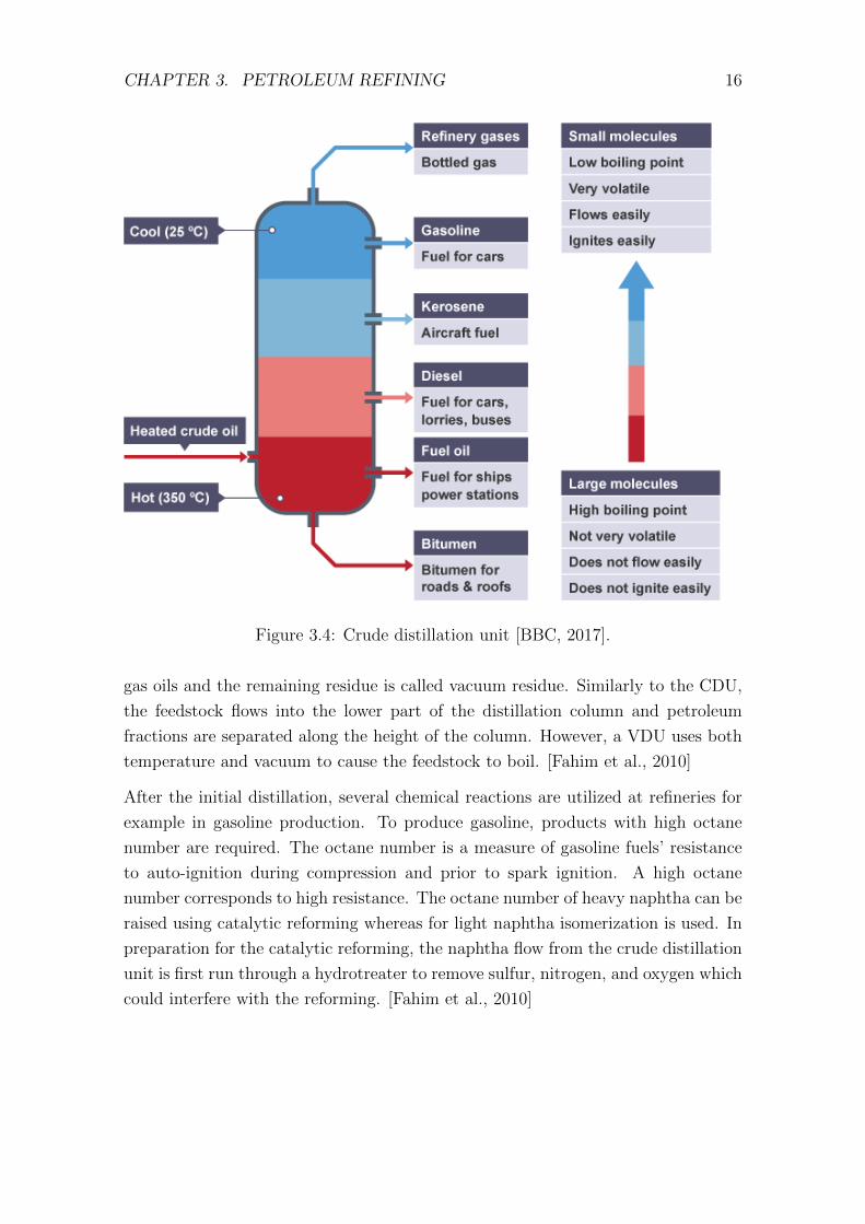
A CDU is an atmospheric distillation unit that separates crude oil into petroleum
fractions. The operating principles of a CDU are illustrated in Figure 3.4. The
temperature in the unit is highest at the bottom of the column and gradually de-
creases towards the top. Pre-heated crude oil is fed into the CDU where most of
CHAPTER 3. PETROLEUM REFINING 15
Figure 3.3: A complex refinery setup [Leffler, 2008].
its hydrocarbon components are vaporized. These components rise up to the cooler
parts of the column. The lighter the hydrocarbon molecules are the higher they rise
in the column before condensing back into liquid. Different parts of the column are
separated by trays that allow vaporized hydrocarbons to flow upwards but prevent
liquid hydrocarbons from flowing downwards. When a hydrocarbon reaches the sec-
tion of the column where it condenses, it flows out as a liquid side stream. Therefore,
different hydrocarbons can be extracted at different parts of the distillation column.
Note that the process is not ideal and these petroleum fractions still contain some
amounts of undesired hydrocarbons. [Fahim et al., 2010]
A vacuum distillation unit (VDU) separates more of the valuable distillates from the
heaviest bottom oil fraction of the CDU. These distillates are referred to as vacuum
CHAPTER 3. PETROLEUM REFINING 16
Figure 3.4: Crude distillation unit [BBC, 2017].
gas oils and the remaining residue is called vacuum residue. Similarly to the CDU,
the feedstock flows into the lower part of the distillation column and petroleum
fractions are separated along the height of the column. However, a VDU uses both
temperature and vacuum to cause the feedstock to boil. [Fahim et al., 2010]
After the initial distillation, several chemical reactions are utilized at refineries for
example in gasoline production. To produce gasoline, products with high octane
number are required. The octane number is a measure of gasoline fuels’ resistance
to auto-ignition during compression and prior to spark ignition. A high octane
number corresponds to high resistance. The octane number of heavy naphtha can be
raised using catalytic reforming whereas for light naphtha isomerization is used. In
preparation for the catalytic reforming, the naphtha flow from the crude distillation
unit is first run through a hydrotreater to remove sulfur, nitrogen, and oxygen which
could interfere with the reforming. [Fahim et al., 2010]

CHAPTER 3. PETROLEUM REFINING 17
3.4 Refining Margin
The profitability of running a refinery includes several factors. In the scope of this
thesis, these factors must be understood well enough to decide which are relevant
to the optimization model. Figure 3.5 illustrates historical import prices to Finland
for crude oil, middle distillates, and fuel oil. It is evident from the figure that the
price gap between crude oil and products refined from it is not constant. This is
one factor that affects the profitability of refineries and the effect can be different
on refineries of different complexity, location, and so on.
Figure 3.5: Historical import prices of oil to Finland [Statistics Finland, 2017].
Refinery profitability can be measured by a refining margin which depicts the profits
per unit of crude oil processed. In the petroleum industry, the amount of petroleum
goods are measured in both mass and volume. A common unit of measure for a
volume of a petroleum good is the barrel which is defined as 158.9873·10−3 m3 [Fahim
et al., 2010] [National Institute of Standards and Technology, U.S. Department of
Commerce, 2008].
Three different refining margins are defined by Fahim et al. [2010], namely gross
margin, net margin, and cash margin. Gross margin is calculated by reducing the
cost of the purchased crude oil from the combined value of the refined products. Net
margin can be derived from gross margin by reducing variable refining costs. Cash
margin is obtained in a similar manner by reducing fixed costs from the net margin.
CHAPTER 3. PETROLEUM REFINING 18
Therefore a positive cash margin indicates that the refinery is profitable [Fahim
et al., 2010]. However, a refining margin can be deceptive. A refinery analyzed
individually could have a low refining margin even if it contributes strongly to the
refining margin of a company. This is because some intermediate products could be
delivered to a differently configured refinery for further processing. In such a case
the refining margin of this other refinery could be very high. This is one reason
why there are synergy benefits for a company for owning several refineries. The
calculation of the different refining margins is summarized below.
Gross margin = Value of products− Cost of crude (3.1)
Net margin = Gross margin− Variable refining costs (3.2)
Cash margin = Net margin− Fixed costs (3.3)
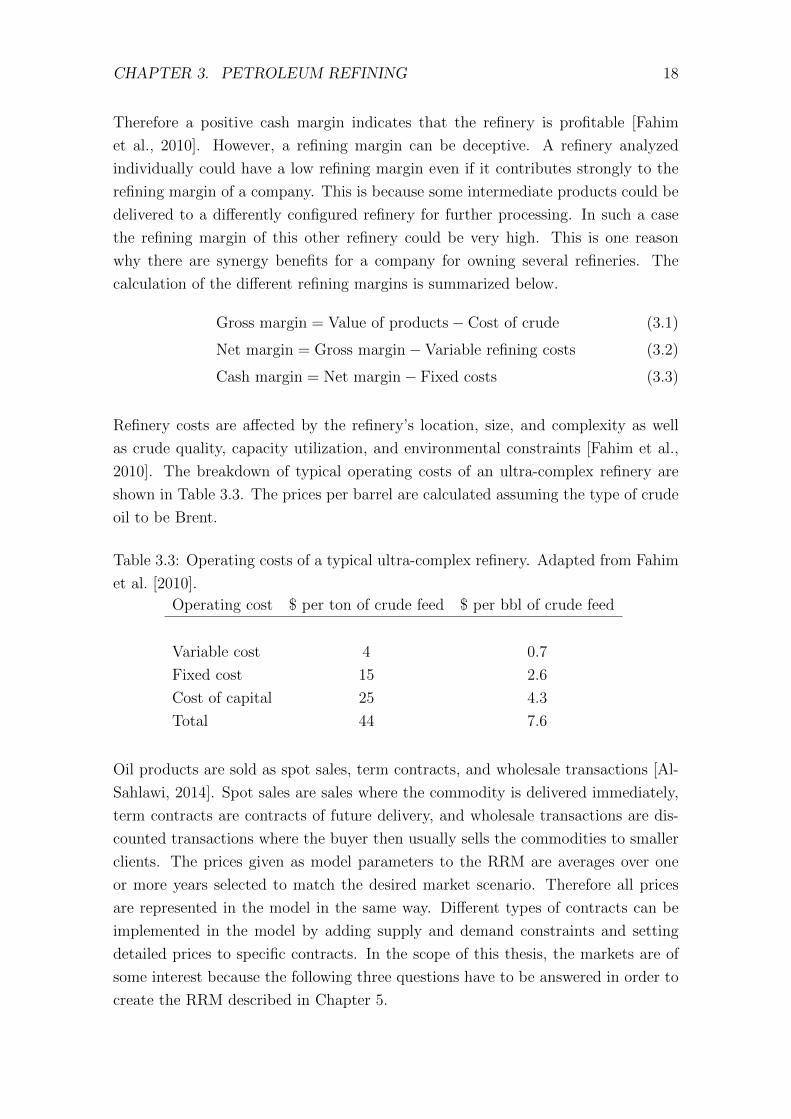
Refinery costs are affected by the refinery’s location, size, and complexity as well
as crude quality, capacity utilization, and environmental constraints [Fahim et al.,
2010]. The breakdown of typical operating costs of an ultra-complex refinery are
shown in Table 3.3. The prices per barrel are calculated assuming the type of crude
oil to be Brent.
Table 3.3: Operating costs of a typical ultra-complex refinery. Adapted from Fahim
et al. [2010].
Operating cost $ per ton of crude feed $ per bbl of crude feed
Variable cost 4 0.7
Fixed cost 15 2.6
Cost of capital 25 4.3
Total 44 7.6
Oil products are sold as spot sales, term contracts, and wholesale transactions [Al-
Sahlawi, 2014]. Spot sales are sales where the commodity is delivered immediately,
term contracts are contracts of future delivery, and wholesale transactions are dis-
counted transactions where the buyer then usually sells the commodities to smaller
clients. The prices given as model parameters to the RRM are averages over one
or more years selected to match the desired market scenario. Therefore all prices
are represented in the model in the same way. Different types of contracts can be
implemented in the model by adding supply and demand constraints and setting
detailed prices to specific contracts. In the scope of this thesis, the markets are of
some interest because the following three questions have to be answered in order to
create the RRM described in Chapter 5.
CHAPTER 3. PETROLEUM REFINING 19
1. For each refinery, which markets can it reasonably access?
2. For each refinery, what are the transportation costs associated with each of
the markets it is involved in?
3. For each market, what is the maximum supply and demand of each type of
goods?
These can be answered based on historical transaction observations, geographical
location, and local infrastructure of each refinery.
In practice, when the RRM is ran, it will provide such a cash margin for each refinery
that includes the following costs: crude oil and other import costs, refinery operating
expenses, and transportation costs. The refinery operating costs include electricity,
steam, and catalysts as well as workforce cost. This calculated cash margin is used
for ranking the refineries and the refining companies. Alternatively, a gross or net
margin can be selected if so desired. The questions given above are essential in
determining the parameters that affect the ranking solution.
3.5 Supply Chain Planning
This section introduces supply chain planning (SCP) and explains how the RRM
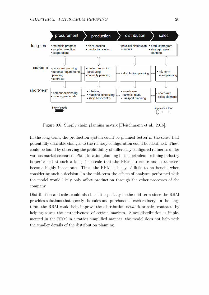
could be utilized in different processes and subprocesses in SCP. Figure 3.6 depicts a
SCP matrix where subprocesses such as ‘cooperations’ are organized by term length
(rows) and by parent process (columns). The terms are defined as follows. Long-
term planning covers strategic decisions noticeable over periods of several years.
Medium-term planning outlines regular operations for periods of 6 to 24 months.
Short-term planning concerns detailed operational plans for up to three months
into the future. The RRM is designed to be run for periods of one or more years.
Therefore it aims to support mid to long-term planning. Next, the long-term and
mid-term rows of the supply chain planning matrix are analyzed to determine which
of the listed activities might benefit from the use of the RRM. [Fleischmann et al.,
2015]
In the procurement parent process, long-term planning could benefit in the activities
of materials program and supplier selection. The RRM can provide insight to the
profitability and demand of different crude oils from different suppliers. This could
be analyzed by observing the changes in the crude palettes and profitability of
different refineries in the RRM. In the mid-term, material requirements and contracts
could benefit from similar analysis.
CHAPTER 3. PETROLEUM REFINING 20
Figure 3.6: Supply chain planning matrix [Fleischmann et al., 2015].
In the long-term, the production system could be planned better in the sense that
potentially desirable changes to the refinery configuration could be identified. These
could be found by observing the profitability of differently configured refineries under
various market scenarios. Plant location planning in the petroleum refining industry
is performed at such a long time scale that the RRM structure and parameters
become highly inaccurate. Thus, the RRM is likely of little to no benefit when
considering such a decision. In the mid-term the effects of analyses performed with
the model would likely only affect production through the other processes of the
company.
Distribution and sales could also benefit especially in the mid-term since the RRM
provides solutions that specify the sales and purchases of each refinery. In the long-
term, the RRM could help improve the distribution network or sales contracts by
helping assess the attractiveness of certain markets. Since distribution is imple-
mented in the RRM in a rather simplified manner, the model does not help with
the smaller details of the distribution planning.
CHAPTER 3. PETROLEUM REFINING 21
3.6 Petroleum Refining in the Refinery Ranking
Model
The topics covered in this chapter are essential for the design of the RRM described
in Chapter 5. Combined with the optimization methods introduced in Chapter 4
and real-world reference data of the refineries and markets, they enable the creation
of the RRM.
In the RRM, the petroleum refining industry is described from crude oil purchases
to end product sales. The separation of crude oil into petroleum fractions and
further processing into end products is described through detailed functions. These
functions are based on the properties of the crude oils, the specifications of the end-
products, and the theory of how different process units operate. How the process
units are configured into a refinery affects the ratio of end products obtained by the
refinery and therefore also the refining margin. Since the economic aspect is also
central, an understanding of the refining margin is required to properly describe
the goals of the refining companies. Since supply and demand play a major role in
any market, understanding of the petroleum market is also required for successful
utilization of the RRM. Finally, understanding of the SCP allows identification of
potential benefits the RRM could offer.
Chapter 4
Optimization Methods
This chapter introduces methods used in MOO and especially in MOLP. Addition-
ally, these methods are compared with each other and those feasible for the Refinery
Ranking Model (RRM) are identified.
4.1 Multi-Objective Optimization
This thesis discusses a MOO problem. For MOO problems with conflicting objective
functions, a completely optimal solution does not always exist. Therefore, Pareto-
optimality is used as a solution concept. Consider a set of objective functions fi(x),
i = 1, 2, 3, ..., where x ∈ X is a vector of decision variables. Each objective function
fi(x) is to be minimized. A point x∗ ∈ X is said to be a Pareto-optimal solution
if and only if there exists no other x ∈ X for which fi(x) ≤ fi(x∗) for all i and
fi(x) 6= fi(x∗) for some i [Sakawa et al., 2013]. A point x∗ is said to be a weakly
Pareto-optimal solution if and only if there exists no other x for which fi(x) < fi(x∗)
for all i [Sakawa et al., 2013]. Pareto-optimality and weak Pareto-optimality are
presented graphically in Figure 4.1. The Pareto-optimal solutions form a Pareto
front [Miettinen, 1999]. In Figure 4.1 the Pareto front is the line connecting the
labeled Pareto-optimal solutions.
Several methods for solving MOO problems exist. These can be classified into four
classes which are no-preference methods, a posteriori methods, a priori methods,
and interactive methods. [Miettinen, 1999]
22

CHAPTER 4. OPTIMIZATION METHODS 23
Figure 4.1: Pareto-optimal and weak Pareto-optimal solutions to a minimization
problem with two objective functions [Yoshimi et al., 2012].
No-preference methods are the most simplistic class as they do not assume prefer-
ence relations between Pareto-optimal solutions. The three other classes require a
decision maker whose preferences are utilized to form criteria on how to select a
preferred solution from a set of Pareto-optimal solutions. This can mean, e.g., that
preference relations are created between the different conflicting objective functions
such that an increase in one is deemed more desirable than an equal increase in an-
other. In a posteriori methods, Pareto-optimal solutions are generated first and the
decision maker selects a satisfactory solution afterwards. A posteriori methods are
often computationally heavy. In a priori methods, the decision maker’s preferences
are surveyed in advance and implemented into the solution method. Interactive
methods are iterative in nature. Practically, this means that Pareto-optimal solu-
tions are generated and improved based on the input from the decision maker until
the decision maker accepts a solution. [Miettinen, 1999]
To find (weak) Pareto-optimal solutions to a MOLP problem, a scalarization method
is used. These methods are introduced in Section 4.2 and the choice of method
used in the RRM is explained in Section 4.3. Some of these methods can be used
in different ways so that they belong to different classes of solution methods. It
is also noteworthy that some methods for solving MOO problems can find all the
Pareto-optimal solutions while others can only find Pareto-optimal extreme solutions

CHAPTER 4. OPTIMIZATION METHODS 24
[Miettinen, 1999].
4.2 Multi-Objective Linear Programming
As explained in Chapter 1, the problem presented in this thesis is formulated as
a MOLP problem although the final model in the software is a non-linear MOO
problem. For MOLP problems, there are several solution concepts from which to
choose from. First, some scalarization methods for MOLP problems are introduced.
These methods are used to characterize Pareto-optimal solutions such that there is a
non-arbitrary rule for selecting among the solution candidates [Sakawa et al., 2013].
The following three methods will be introduced: the weighting method, the weighted
minimax method, and the constraint method. Then, linear goal programming is
discussed as an alternative method. Methods that rely on using a certain algorithm
are of no interest in the scope of this thesis since there is no control over the algorithm
used by the selected software.
A general MOLP problem can be formulated as follows:
minx∈X
z(x) = (z1(x), ..., zk(x)) , (4.1)
where z1(x), ..., zk(x) are k distinct objective functions of the decision variable vector
x = (x1, ..., xn)T and
X = {x ∈ IR | Ax ≤ b, x ≥ 0} (4.2)
is the linearly constrained feasible region where A is an m × n matrix and b is a
m-vector [Sakawa et al., 2013].
In the weighting method, a weighted sum of all the objective functions is minimized
(or maximized). It is defined by
minx∈X
wz(x) =k∑
i=1
wizi(x) , (4.3)
where w = (w1, ..., wk) ≥ 0, w 6= 0 is a vector of weighting coefficients. The
benefit of the weighting method over some of the others is that it guarantees Pareto-
optimality rather than only weak Pareto-optimality. [Sakawa et al., 2013]
The weighted minimax method looks for a solution where the greatest objective
function value is minimized according to
min v (4.4)
subject to wz(x) ≤ v ,

CHAPTER 4. OPTIMIZATION METHODS 25
Figure 4.2: If f2(x) is constrained between a and b only a weak Pareto-optimal
solution to the original problem can be found. Adapted from Yoshimi et al. [2012].
where v is an auxiliary variable [Sakawa et al., 2013]. Only weak Pareto-optimality
can be guaranteed by the weighted minimax method [Sakawa et al., 2013]. From
Figure 4.1 it can be observed that this method results in solutions in the middle
region of the Pareto front since large values are avoided for all objective functions.
For a maximization problem, the equivalent would be a maximin problem where the
minimum objective function value is maximized. This could be beneficial for the
RRM since there would be a good chance of avoiding solutions where some refineries
are given either unrealistically high or low emphasis.
In the constraint method, one of the objective functions is selected and the others are
treated as inequality constraints. Only weak Pareto-optimality can be guaranteed
by the constraint method [Sakawa et al., 2013]. This is demonstrated in Figure 4.2
where objective function f2(x) is turned into a constraint and limited to only get
values in the interval [a, b] while objective function f1(x) is minimized. Since all the
Pareto-optimal solutions are below f2(x) = a and therefore outside the new feasible
region, only a weak Pareto-optimal solution can be found.

Table 4.1: Summary of different MOLP methods.
Wei
ghti
ng
met
hod
Wei
ghte
dm
inim
ax
Con
stra
int
met
hod
Lin
ear
goal
pro
gram
min
g
Advantages:
Pareto-optimal solutions x
More balanced solutions x
Specific undesired solutions can be ruled out x
Disadvantages:
Need to assign desired weighting coefficients x
Only weak Pareto-optimality guaranteed x x
Need to assign desired values for all objective functions x
In linear goal programming, the decision maker sets aspiration levels for the objective
functions and then the deviation from these targets is minimized [Sakawa et al.,
2013]. The advantages and disadvantages of each method are summarized in Table
4.1.
4.3 Selection of Multi-Objective Linear Program-
ming Methods
In this section, a rationale is provided for the choice of method for choosing between
Pareto-optimal solutions in the RRM. General attributes of such methods were
described in Section 4.2. Pareto-optimal solutions, weakly Pareto-optimal solutions,
and optimization methods for finding these were also introduced in Section 4.2.
When selecting between the alternative methods, it is crucial to take into account
any limitations imposed by the choice of software. In this case, the Spiral Suite1
software is used to implement the model.
Since the nature of the problem at hand is finding realistic scenarios and an exact
correct outcome can not be known, there is no single correct method for selecting
between Pareto-optimal solutions. It is not trivial to say whether weak Pareto-
1 Spiral Suite by AVEVATM

CHAPTER 4. OPTIMIZATION METHODS 27
optimality will suffice. Companies do not have incentive to change their behavior
unless their own profits would increase and therefore a weak Pareto-optimal solution
would be possible. However, a company would never be content with a situation
where its own actions could increase its profit. Thus, a weak Pareto-optimal solution
might exist that would not depict a realistic situation in the model. Such a solution
is undesirable and therefore a method that yields strong Pareto-optimal solutions is
preferable.
A single company can not select the solution of their choice. Instead, the RRM
is used to give insight to possible market scenarios. This would suggest using a
no-preference method for the optimization method. No-preference methods are also
the most simple method class and thus the easiest to implement. However, if the
model exhibits behavior such that some refineries are emphasized excessively, it
might be preferable to adjust the model performance by giving such a refinery lower
preference. A priori methods would allow this and therefore be more robust. Future
development of the RRM could utilize some other method class. For example,
regular use of the model and comparison of its results to reality could allow an
analyst to develop an expertise sufficient for acting as the decision maker required
for the other method classes.
To make use of an a priori method, one of the methods introduced earlier in this
chapter is selected. In the scope of this thesis, linear goal programming is hardly a
reasonable approach since the aim of the analysis is to produce the very knowledge
required as an input for this method. However, the decision maker could have a
good idea of the realistic levels of some objective functions. Therefore, this method
could possibly be utilized to some degree in a more complex future implementation
of the model. Only the three scalarization methods remain as potential methods of
choice.
The simplest scalarization method for the problem would be the weighting method.
If all refineries are given equal weights, the RRM is equivalent to a no-preference
model. Adjusting the weights turns it into an a priori model instead. Desirable
weights could be found through iteration by comparing the model results to existing
data after every change in the weighting coefficients.
Another scalarization method that could be easily implemented is the constraint
method. This would mean adding a constraint that sets the refining margins of all
but one company between some limits determined for each company. Whether or
not such a constraint is added, the flow rate of each refinery will be constrained be-
tween two values determined by the properties of the refinery’s process units. This is
a technological constraint since a sufficient flow rate is required to operate the CDU
[Fahim et al., 2010]. A refinery will run on at least the technical minimum flow rate
even if the refinery is temporarily not profitable since the shutdown and restarting
of a refinery is an expensive and complicated process [Lenahan, 2006]. Further-
more, there is a need for maintaining a sufficient supply of petroleum products to
meet international regulations and national requirements in the event of disruptions
[Ministry of Economic Affairs and Employment, Finland, 2018]. Therefore, shutting
down a refinery is rare and the bounds of a refinery’s refining margin are defined
by the minimum and maximum feed rates of its process units, mainly the CDU.
Thus, the objective functions of all but one company could simply be removed and
there would still be a valid LP problem which would yield somewhat realistic results.
However, these results could be only weakly Pareto-optimal and unrealistic in the
scale of the entire network model. The company whose gross margin is maximized
would likely enjoy an unrealistic advantage. In theory, the potentially unrealistic
weak Pareto-optimal solutions could be ruled out by selecting the constraints con-
veniently. In practice, however, it can not be known what the perfect constraint
choices would be. It might be possible to improve the results by selecting tighter
constraints based on an overview of the current price set. For example, if a cer-
tain refinery is know to do well under certain market prices, then its minimum flow
rate could be set higher than normal when running scenarios with those beneficial
prices.
The weighted maximin method on the other hand could not be implemented using
the Spiral Suite1 software. There is no way to formulate this kind of an objective
function in the software since it only maximizes the total sum of the refining margins
of all refineries. In the case of the constraint problem, this can be circumvented by
limiting the flow rates and setting prices of the raw materials, transportation, and
products of the constraint refineries to zero. This way the sum of all refineries’
margins are analogous to that of the refinery whose margin is to be maximized.
For the maximin problem, such a workaround is not possible since in the software
there is no way to implement the required auxiliary variable v that was described
in Equation 4.4. The function to be maximized must explicitly include z(x).
Under these limitations, the conclusion is that the weighting method would be fitting
for the RRM. Additionally, the constraint method can be easily implemented and
could be useful under some circumstances. The presumption is that the weighting
method could be used to simulate the effect of different market scenarios on the gen-
eral profitability of the industry and the ranking of different refineries. Furthermore,
it is presumed that the constraint method could be used to create best case scenarios
for an individual refinery. The clear downside of the constraint method is that all
but one refinery are highly susceptible to sub-optimal behavior when compared to
1 Spiral Suite by AVEVATM

CHAPTER 4. OPTIMIZATION METHODS 29
their real-life behavior.
Chapter 5
The Refinery Ranking Model
The Refinery Ranking Model (RRM) is built to analyze the profitability of several
refineries and refining companies given specific market prices for crude oils and
petroleum products. It depicts a system that contains several refineries and market
nodes. These are linked together to form a network where goods are traded based on
supply and demand. The RRM is used to analyze time periods of one or more years.
This chapter presents the structure and rationale of the model. Since the model
contains over 17 000 equations and over 16 000 variables these are not presented
individually. The general structure of the model is described in Section 5.1, the
notation used in the model is listed in Section 5.2, and general assumptions and
mathematical formulation of the model are covered in Sections 5.3-5.6. The model
validation is covered in Chapter 6. The RRM is built using Spiral Suite1 software
build version 5.3.
Certain requirements are placed on the RRM. The user of the model has to be able to
study different scenarios by setting the corresponding market prices and optimization
constraints into the model. The optimization constraints include, but are not limited
to, the amounts of raw materials available and end products demanded in different
countries. The model is to be designed in a manner that allows it to be expanded in
the future with relative ease. It consists of a network of refinery models each of which
contains several process unit models. For ease of expansion and maintenance, the
process unit models are built in a generic manner such that each different refinery
can be described using the same process unit models.
1 Spiral Suite by AVEVATM
5.1 General structure
The RRM is formulated as a multi-objective linear programming model. It consists
of 3 companies which own 5 refineries in total. Two of the companies own two
refineries each and one company owns a single refinery. Each company aims to
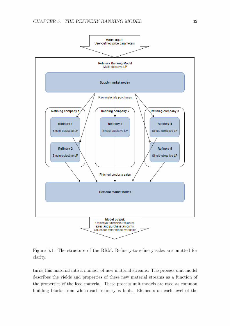
maximize the sum profit of their own refineries. The inputs, outputs, and objective
functions of the model are illustrated in Figure 5.1.
First, the user inputs the market scenario price set into the Spiral Suite1 software.
Then, the RRM aims to maximize the total objective function of the system. The
software runs an optimization algorithm that starts from an arbitrary point. It
then iterates from one potential solution to another staying within the limits set
by the optimization constraints. The algorithm stops once there is indication that
the current solution can not be improved any further. If the weighting method is
used, the total objective function is a weighted sum of refinery objective functions.
If the constraint method is used instead, then the total objective function equals the
sum of objective functions of one or more, but not all, refineries. For the constraint
method the total objective function would most likely be the objective function of a
single refinery or a single refining company. It should be noted that a combination
of the weighting and the constraint method could be used if so desired.
Once the optimization algorithm stops, the model provides a listing of all purchases,
sales, material flows, technical refinery operating parameters, and the net margin
and cash margin of each refinery and consequently each refining company. The cash
margin of a refinery or a refining company matches the respective objective function
if and only if the objective function is given a weight of 1.
The model as a whole consists of three levels. This hierarchy is illustrated in Figure
5.2. The highest level is the refinery network level which links each refinery to
markets and describes supply, demand, and transportation of goods. On this level,
the transportation of goods to and from each refinery is optimized. The second level
contains the LP models of the refineries. On this level, the crude oil entering the
refinery is turned into intermediate products and end products in a manner that
aims to maximize the value added to the products. These refinery LP models are
formed by linking process unit models together as well as to purchases and sales
determined for that particular refinery. The combination of process unit models
in a refinery defines the possible product portfolios of that refinery. The lowest
level contains the linear models of the process units. These models describe the
functionality of individual process units within a refinery. Each process unit takes
in a feed of either crude oil, petroleum fraction, or intermediate product. It then
1 Spiral Suite by AVEVATM
CHAPTER 5. THE REFINERY RANKING MODEL 32
Figure 5.1: The structure of the RRM. Refinery-to-refinery sales are omitted for
clarity.
turns this material into a number of new material streams. The process unit model
describes the yields and properties of these new material streams as a function of
the properties of the feed material. These process unit models are used as common
building blocks from which each refinery is built. Elements on each level of the
CHAPTER 5. THE REFINERY RANKING MODEL 33
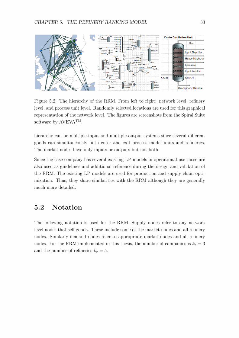
Figure 5.2: The hierarchy of the RRM. From left to right: network level, refinery
level, and process unit level. Randomly selected locations are used for this graphical
representation of the network level. The figures are screenshots from the Spiral Suite
software by AVEVATM.
hierarchy can be multiple-input and multiple-output systems since several different
goods can simultaneously both enter and exit process model units and refineries.
The market nodes have only inputs or outputs but not both.
Since the case company has several existing LP models in operational use those are
also used as guidelines and additional reference during the design and validation of
the RRM. The existing LP models are used for production and supply chain opti-
mization. Thus, they share similarities with the RRM although they are generally
much more detailed.
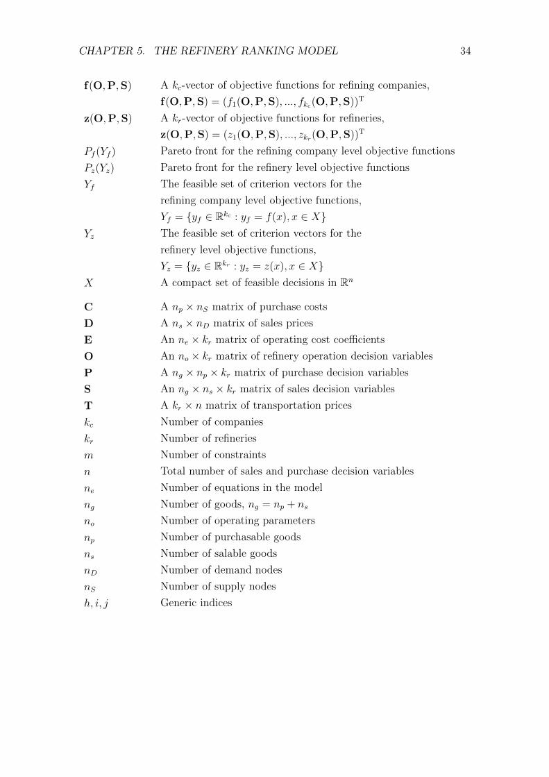
5.2 Notation
The following notation is used for the RRM. Supply nodes refer to any network
level nodes that sell goods. These include some of the market nodes and all refinery
nodes. Similarly demand nodes refer to appropriate market nodes and all refinery
nodes. For the RRM implemented in this thesis, the number of companies is kc = 3
and the number of refineries kr = 5.
CHAPTER 5. THE REFINERY RANKING MODEL 34
f(O,P,S) A kc-vector of objective functions for refining companies,
f(O,P,S) = (f1(O,P,S), ..., fkc(O,P,S))T
z(O,P,S) A kr-vector of objective functions for refineries,
z(O,P,S) = (z1(O,P,S), ..., zkr(O,P,S))T
Pf (Yf ) Pareto front for the refining company level objective functions
Pz(Yz) Pareto front for the refinery level objective functions
Yf The feasible set of criterion vectors for the
refining company level objective functions,
Yf = {yf ∈ Rkc : yf = f(x), x ∈ X}Yz The feasible set of criterion vectors for the
refinery level objective functions,
Yz = {yz ∈ Rkr : yz = z(x), x ∈ X}X A compact set of feasible decisions in Rn
C A np × nS matrix of purchase costs
D A ns × nD matrix of sales prices
E An ne × kr matrix of operating cost coefficients
O An no × kr matrix of refinery operation decision variables
P A ng × np × kr matrix of purchase decision variables
S An ng × ns × kr matrix of sales decision variables
T A kr × n matrix of transportation prices
kc Number of companies
kr Number of refineries
m Number of constraints
n Total number of sales and purchase decision variables
ne Number of equations in the model
ng Number of goods, ng = np + ns
no Number of operating parameters
np Number of purchasable goods
ns Number of salable goods
nD Number of demand nodes
nS Number of supply nodes
h, i, j Generic indices
CHAPTER 5. THE REFINERY RANKING MODEL 35
5.3 Assumptions
Next, the assumptions and abstractions made in the design of the RRM are de-
scribed.
The model covers a limited set of refineries which, in reality, function as a part of a
world-wide system of refineries where each individual agent is affected by the system
as a whole. The external agents are described as markets that have constant supply
and demand and limit the demand of goods from internal agents based on the actual
sales figures in the reference data. These external supply and demand are model
parameters and are in addition to any supply and demand of the same goods that
the refineries may provide themselves.
For simplicity, the number of goods in the model is limited to include only those
that have a considerable impact on the included refineries. Other goods are either
ignored or pooled into these chosen categories. As a result of reduced number of
different goods the refineries themselves have also been simplified in the sense of
removing process units and streams that deal with goods or characteristics that
are not included in the model. This is also required because the data available of
some refineries is not detailed enough for accurately describing some of the more
elaborate processes. An additional benefit of simplified refinery models is ease of
model upkeep. For further ease of upkeep, generic process unit models are used such
that each refinery model is built of the same constituent parts as the others. To
eliminate redundant solution options the model is designed such that each refinery
has access only to the markets that they would realistically get involved with in the
real world. This considerably reduces the number of equations in the model.
In Section 3.2, it was stated that in the short run the change in crude oil production
is only 2% of the change in crude oil price. As a result it is assumed that the user
can select crude oil prices for their chosen scenario without needing to change the
constraints of available crude oil. It was also stated that the demand for petroleum
products is inelastic with respect to price. Therefore, the user can also change the
price of these products without changing the demand constraints of the markets.
Thus, the supply and demand of the markets is assumed constant and does not
require updating when changing the values of the price parameters. The supply and
demand of the refineries in the RRM changes from solution to solution.
In forming the constraints of the problem it is assumed that each refinery sells all
their products instead of having an inventory where they might store some of the
products. Such an option could be added to the model in the future but in the
CHAPTER 5. THE REFINERY RANKING MODEL 36
scope of this thesis this approach depicting long-term mean throughput is deemed
sufficient. Furthermore, the model is assumed to be run for periods divisible by one
year. In this way, average production and demand can be used instead of accounting
for seasonal changes.
For simplicity, a constant price for each product on each market is assumed. In
addition, transportation costs apply and are determined by the supply and demand
locations. An exception is one market region where two different price levels are
defined such that once the initial demand is filled the price drops but the secondary
demand is infinite. This is to ensure all products can be sold somewhere in the model
since goods can not be stored at the refineries in the model as stated previously.
Furthermore, the problem at hand has network optimization features in the form of
a transportation problem. The network qualities of the problem do not cause issues
as long as the implementation does not include zero-cost transfers between nodes
such that they would create loops where the algorithm might become stuck.
5.4 Decision Variables
The decision variables include the purchases P, sales S, and operating parameters O
for each refinery. The most central decision variables in the model are the sales and
purchases. Each combination of a good, origin, and destination is represented by a
decision variable which represents either a sale to market, a purchase from market,
or a transfer between refineries. These make up most of the decision variables in the
model while refinery operating parameters amount for only a small fraction. The
refinery operating parameters are used to adjust the product palette of a refinery by
running the process units in alternative operating modes or directing some hydro-
carbon flows to different process units. Only some process units and hydrocarbon
flows have such alternative processing options.
5.5 Objective Functions
Consider a vector of refinery objective functions z(O,P,S). Let Oh,j denote the
value of operating parameter h of refinery j. Let Ph,i,j denote the amount of good
h purchased from market i by refinery j. Let Sh,i,j denote the amount of good h
sold to market i by refinery j. Let Dh,i denote the price of a unit of good h sold to
demand node i. Let Ch,i denote the cost of a unit of good h purchased from supply

CHAPTER 5. THE REFINERY RANKING MODEL 37
node i. Let Th,i,j denote the cost per unit of good h transported between market
i and refinery j regardless of direction. Let Eh,j denote the operating expense per
unit of operating parameter value for operating parameter h at refinery j. Then,
each objective function is of the form
zj(O,P,S) =
ng∑h=1
nD∑i=1
Sh,i,jDh,i −ng∑h=1
nS∑i=1
Ph,i,jCh,i
−ng∑h=1
nN∑i=1
(Sh,i,j + Ph,i,j)Th,i,j −no∑h=1
Oh,jEh,j , (5.1)
where j = 1, ..., kr, the first term is the total sales income, the second the total pur-
chasing costs, the third the total transportation costs, and the fourth the operating
costs, respectively. The refinery objective functions zj(O,P,S) correspond to refin-
ery cash margins. The refining company objective functions fj(O,P,S) correspond
to the cash margins of refining companies and equal the sum of the refinery cash
margins for that company’s refineries. When the operating costs terms are set to
zero the objective functions correspond to gross margins instead.
5.6 Constraints
There is a set of constraints associated with every level of the model. On the process
unit level, each process unit model has a set of built-in equality constraints such as
sulfur concentration in the naphtha fraction is equal to 0.01 + 0.2α, where α is the
sulfur concentration in the input feed. On the refinery model level and the refinery
network level, the purchases and sales of each refinery are described as equality
and inequality constraints such as the Urals crude oil purchase of refinery 3 must
be greater than or equal to 1000 barrels per day. These are due to geographical
location, refinery configuration, and market supply and demand.
Each refinery model is built using the same generic process unit model options, some
of which are presented in Table 3.2. Crude Distillation Unit (CDU) and Vacuum
Distillation Unit (VCU) are described using a different technical solution than the
other process units. Regardless of which solution is used, each process model is
specified to have a number of input feeds and petroleum fraction outputs. Each of
these process units also has minimum and maximum feed rate parameters that are
defined by their physical specifications.
As explained in Section 5.3 each refinery is assumed to sell all their products which
means that there is an equality constraint for each product of each refinery such that
CHAPTER 5. THE REFINERY RANKING MODEL 38
the sum of sales of any particular product must be equal to the produced amount
of that product.
The markets in the model can be divided into crude oil markets from which the
refineries buy raw materials and product markets to which refineries sell their prod-
ucts. Some markets might always buy at least or at most a certain amount of some
products which is manifested as inequality constraints.
Chapter 6
Validation of the Refinery Ranking
Model
This chapter describes the validation of the Refinery Ranking Model (RRM) such
that it can be stated whether the results match the reference data and whether solu-
tions are obtained in a robust and timely manner. Firstly, it is determined whether
the model can reproduce the cash margins of each refinery and refining company
in the reference data given the market prices in the reference data. Secondly, the
robustness and solution time of the model is tested in order to analyze the practical
usability. Section 6.1 presents the results of each individual refinery model whereas
Section 6.2 delves into the results of the complete RRM where the refinery models
are linked together into a network. Finally, Section 6.3 deals with the robustness
and solution time of both the refinery models and the complete model.
6.1 Validation of the Refinery Linear Program-
ming Models
Each refinery model is an LP model and as such has a single-objective function.
These models can be run separately from the rest of the MOLP RRM. In order
to find out whether these refinery models match the reference data, they are run
individually with the market price set and the material purchases set to match
those in the reference data. In addition, the results from refineries owned by the
case company can be compared to the results of existing LP models which have been
verified to match actual process data over the years. In the case of refineries owned
by the case company, the complexity of the previously existing models is higher than
39
CHAPTER 6. VALIDATION OF THE REFINERY RANKING MODEL 40
that of those created for this thesis. However, the results of the new models should
roughly match those of the older models. In this section, when referring to RRM
results they mean specifically the results of the refinery LP models runs separately
from the rest of the RRM.
The results of each refinery LP model in the RRM are compared to both technical
and economic reference data. The technical reference data specifies the input and
product palettes of each refinery. For example, a refinery might take three different
crude oils as input and produce eight different end products. For ease of comparison,
the input flow of each refinery is scaled such that the total input of petroleum goods
to each refinery is set to 100 kbbl/d. Air and hydrogen are not taken into account
in this input flow and thus the output flows of the refineries can be above 100
kbbl/d. The input crude oil palette in RRM is set to match the reference data when
validating refinerywise results. For the economic reference data, both gross margin
and cash margin are considered. These are scaled such that the gross margin of
Refinery 1 is set to 10 $/bbl and others are adjusted proportionally to that. Thus,
the signs and proportions are maintained.
When considering the product palettes of refineries, it is importance to notice that
there are some differences in how the different petroleum fractions are defined in the
RRM and in the reference data. For example, abstractions had to be made in how
gasoline products are pooled together and in the product specification constraints.
Furthermore, as explained in Section 3.1, there is overlap in the different petroleum
fractions. Since there is no precise knowledge on how these abstractions are made
in the reference data, there are bound to be differences between the RRM and the
reference data. When comparing the product palette of a refinery in RRM to its
counterpart in the reference data, it is worth looking at each product individually but
also comparing the three broader main categories to each other. These categories are
heavy products, middle distillates, and light products. It was stated in Section 3.1,
that lighter products are generally more valuable than heavier ones and that higher
sulfur concentration reduces value. Thus, products within the same main category
are often of similar value. Figure 6.1 illustrates the product palettes of each refinery
in the reference data and in the RRM. Heavy product are presented in shades of
brown whereas middle distillates are red and light products blue. The product
labeled ‘loss’ refers to the material flows that are directed to combustion instead
of being sold as end products. These belong to the light products category since
they are mostly gases. Both the reference data and the RRM actually contain more
products than shown here but further complexity would lend little added benefit to
the analysis of the results.

CHAPTER 6. VALIDATION OF THE REFINERY RANKING MODEL 41
Figure 6.1: The product palettes of each refinery in the reference data and in the
RRM. Heavy products are illustrated in shades of brown, middle distillates in shades
of red, and light products in shades of blue.
Figure 6.1 shows that for refineries 1, 3, and 5 the rough categorization of the product
palette yields very similar results in the RRM and the reference data. For Refinery
2, the RRM clearly gives a higher amount of heavy products at the expense of light
products. However, this refinery has gone through a change of refinery configuration
after collecting the reference data. It is decided that the current configuration should
be implemented in the RRM even if it complicates model validation. In the new
configuration, a smaller proportion of heavy fractions is converted into light products
which explains the change in the product palette. For refinery 4, the RRM gives
higher amounts of light products and less middle distillates than the reference data.
Investigation reveals two potential factors for the difference. One factor is that
the general process unit models do not necessarily represent the changes in density
during the process for this particular refinery. If, in reality, the density of the middle
CHAPTER 6. VALIDATION OF THE REFINERY RANKING MODEL 42
distillates is lower and that of light products is higher that could explain a deviation
similar to that shown in the figure. However, the possible mismatch in densities is
unlikely to be sufficient to explain a deviation of such a proportion. The second
potential cause of the difference between the RRM result and the reference data lies
in the data that describes the crude oils. If the composition of a crude oil has major
differences between the RRM and the reference data then the petroleum fraction
yields will inevitably differ. In such a case, only making changes to the refinery model
configuration can remove this difference from the results. Naturally, this would then
be inaccurate compared to the configuration in the reference data. It is also possible
that there is an error in the reference data such that the refinery configuration and
product palette in the reference data do not match each other.
Taking a look at the products on the more precise level, it is clear that there is
some difference in the ratios of the actual products between the reference and the
RRM. These are generally caused by minor differences in the process unit models
and the product specifications between RRM and the reference data. For example,
since the different refinery models in the RRM use the same process unit models,
the kerosene fraction that comes from the CDU differs between RRM and reference
for Refinery 5. If a CDU is tailored to match the reference data for Refinery 5,
then this difference can easily be accounted for. Concerning the effect of product
specifications, Refinery 3 allows for a good example. The sum of gasoil and diesel
produced at Refinery 3 is quite well matched between the reference data and the
RRM. The product specifications for gasoil are much more lenient than for diesel. If
possible, a refinery will attempt to process all their gasoil into more valuable diesel
but in some cases the specifications, e.g. sulfur concentration, can not meet the
specification if all of the gasoil is processed. Thus, some of the gasoil needs to be
sold as is.
A comparison of the refining margins of each refinery and refining company are
plotted in Figure 6.2. The blue bars indicate gross margins and the red ones cash
margins. Darker bars indicate reference data and lighter bars RRM results. For
each individual refinery and refining company, the difference between the reference
bar and the RRM result bar is the same for the gross margins and the cash margins.
Since cash margin is gross margin minus operational expenses, this indicates that
the operational expenses in the RRM match exactly to those in the reference data.
Calculations show that the operational expenses in the RRM are a precise match
to the reference data. However, it is clear from Figure 6.2 that in many cases the
difference between the reference and RRM bars is considerable. For the refineries,
the ranking from the most profitable to the least profitable in the RRM matches the
reference data. When summing the results of the refineries to obtain the results for
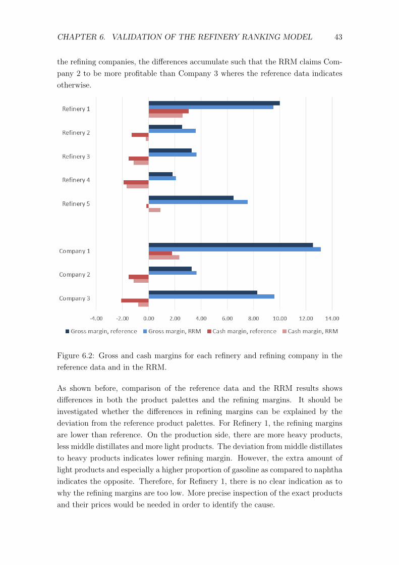
CHAPTER 6. VALIDATION OF THE REFINERY RANKING MODEL 43
the refining companies, the differences accumulate such that the RRM claims Com-
pany 2 to be more profitable than Company 3 wheres the reference data indicates
otherwise.
Figure 6.2: Gross and cash margins for each refinery and refining company in the
reference data and in the RRM.
As shown before, comparison of the reference data and the RRM results shows
differences in both the product palettes and the refining margins. It should be
investigated whether the differences in refining margins can be explained by the
deviation from the reference product palettes. For Refinery 1, the refining margins
are lower than reference. On the production side, there are more heavy products,
less middle distillates and more light products. The deviation from middle distillates
to heavy products indicates lower refining margin. However, the extra amount of
light products and especially a higher proportion of gasoline as compared to naphtha
indicates the opposite. Therefore, for Refinery 1, there is no clear indication as to
why the refining margins are too low. More precise inspection of the exact products
and their prices would be needed in order to identify the cause.
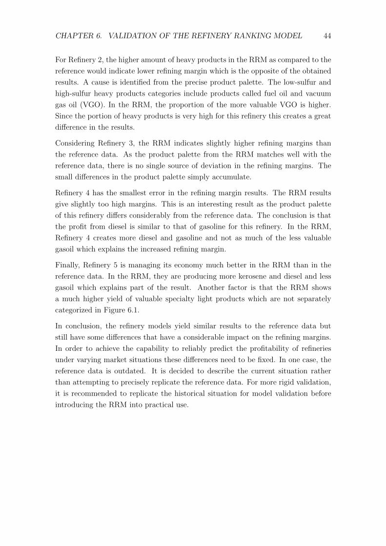
CHAPTER 6. VALIDATION OF THE REFINERY RANKING MODEL 44
For Refinery 2, the higher amount of heavy products in the RRM as compared to the
reference would indicate lower refining margin which is the opposite of the obtained
results. A cause is identified from the precise product palette. The low-sulfur and
high-sulfur heavy products categories include products called fuel oil and vacuum
gas oil (VGO). In the RRM, the proportion of the more valuable VGO is higher.
Since the portion of heavy products is very high for this refinery this creates a great
difference in the results.
Considering Refinery 3, the RRM indicates slightly higher refining margins than
the reference data. As the product palette from the RRM matches well with the
reference data, there is no single source of deviation in the refining margins. The
small differences in the product palette simply accumulate.
Refinery 4 has the smallest error in the refining margin results. The RRM results
give slightly too high margins. This is an interesting result as the product palette
of this refinery differs considerably from the reference data. The conclusion is that
the profit from diesel is similar to that of gasoline for this refinery. In the RRM,
Refinery 4 creates more diesel and gasoline and not as much of the less valuable
gasoil which explains the increased refining margin.
Finally, Refinery 5 is managing its economy much better in the RRM than in the
reference data. In the RRM, they are producing more kerosene and diesel and less
gasoil which explains part of the result. Another factor is that the RRM shows
a much higher yield of valuable specialty light products which are not separately
categorized in Figure 6.1.
In conclusion, the refinery models yield similar results to the reference data but
still have some differences that have a considerable impact on the refining margins.
In order to achieve the capability to reliably predict the profitability of refineries
under varying market situations these differences need to be fixed. In one case, the
reference data is outdated. It is decided to describe the current situation rather
than attempting to precisely replicate the reference data. For more rigid validation,
it is recommended to replicate the historical situation for model validation before
introducing the RRM into practical use.
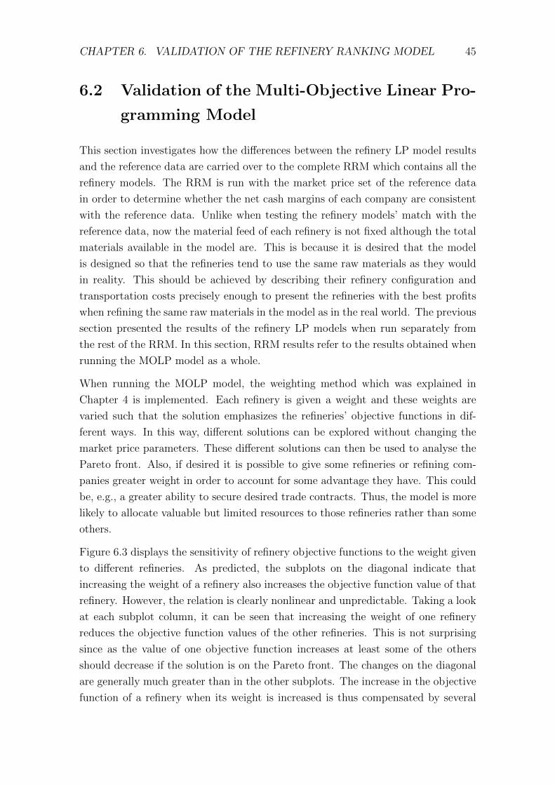
CHAPTER 6. VALIDATION OF THE REFINERY RANKING MODEL 45
6.2 Validation of the Multi-Objective Linear Pro-
gramming Model
This section investigates how the differences between the refinery LP model results
and the reference data are carried over to the complete RRM which contains all the
refinery models. The RRM is run with the market price set of the reference data
in order to determine whether the net cash margins of each company are consistent
with the reference data. Unlike when testing the refinery models’ match with the
reference data, now the material feed of each refinery is not fixed although the total
materials available in the model are. This is because it is desired that the model
is designed so that the refineries tend to use the same raw materials as they would
in reality. This should be achieved by describing their refinery configuration and
transportation costs precisely enough to present the refineries with the best profits
when refining the same raw materials in the model as in the real world. The previous
section presented the results of the refinery LP models when run separately from
the rest of the RRM. In this section, RRM results refer to the results obtained when
running the MOLP model as a whole.
When running the MOLP model, the weighting method which was explained in
Chapter 4 is implemented. Each refinery is given a weight and these weights are
varied such that the solution emphasizes the refineries’ objective functions in dif-
ferent ways. In this way, different solutions can be explored without changing the
market price parameters. These different solutions can then be used to analyse the
Pareto front. Also, if desired it is possible to give some refineries or refining com-
panies greater weight in order to account for some advantage they have. This could
be, e.g., a greater ability to secure desired trade contracts. Thus, the model is more
likely to allocate valuable but limited resources to those refineries rather than some
others.
Figure 6.3 displays the sensitivity of refinery objective functions to the weight given
to different refineries. As predicted, the subplots on the diagonal indicate that
increasing the weight of a refinery also increases the objective function value of that
refinery. However, the relation is clearly nonlinear and unpredictable. Taking a look
at each subplot column, it can be seen that increasing the weight of one refinery
reduces the objective function values of the other refineries. This is not surprising
since as the value of one objective function increases at least some of the others
should decrease if the solution is on the Pareto front. The changes on the diagonal
are generally much greater than in the other subplots. The increase in the objective
function of a refinery when its weight is increased is thus compensated by several
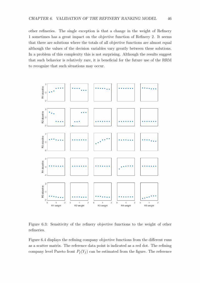
CHAPTER 6. VALIDATION OF THE REFINERY RANKING MODEL 46
other refineries. The single exception is that a change in the weight of Refinery
1 sometimes has a great impact on the objective function of Refinery 2. It seems
that there are solutions where the totals of all objective functions are almost equal
although the values of the decision variables vary greatly between these solutions.
In a problem of this complexity this is not surprising. Although the results suggest
that such behavior is relatively rare, it is beneficial for the future use of the RRM
to recognize that such situations may occur.
Figure 6.3: Sensitivity of the refinery objective functions to the weight of other
refineries.
Figure 6.4 displays the refining company objective functions from the different runs
as a scatter matrix. The reference data point is indicated as a red dot. The refining
company level Pareto front Pf (Yf ) can be estimated from the figure. The reference
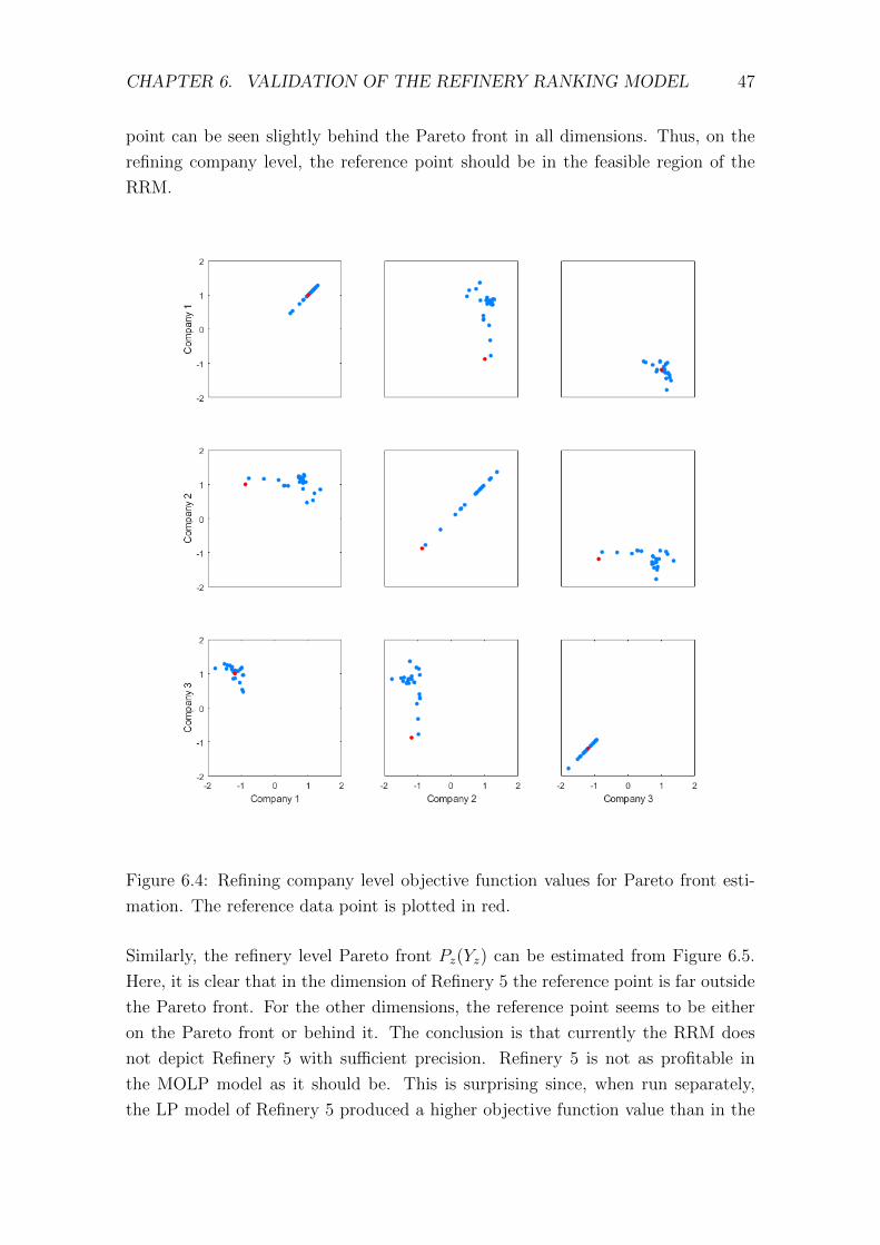
CHAPTER 6. VALIDATION OF THE REFINERY RANKING MODEL 47
point can be seen slightly behind the Pareto front in all dimensions. Thus, on the
refining company level, the reference point should be in the feasible region of the
RRM.
Figure 6.4: Refining company level objective function values for Pareto front esti-
mation. The reference data point is plotted in red.
Similarly, the refinery level Pareto front Pz(Yz) can be estimated from Figure 6.5.
Here, it is clear that in the dimension of Refinery 5 the reference point is far outside
the Pareto front. For the other dimensions, the reference point seems to be either
on the Pareto front or behind it. The conclusion is that currently the RRM does
not depict Refinery 5 with sufficient precision. Refinery 5 is not as profitable in
the MOLP model as it should be. This is surprising since, when run separately,
the LP model of Refinery 5 produced a higher objective function value than in the
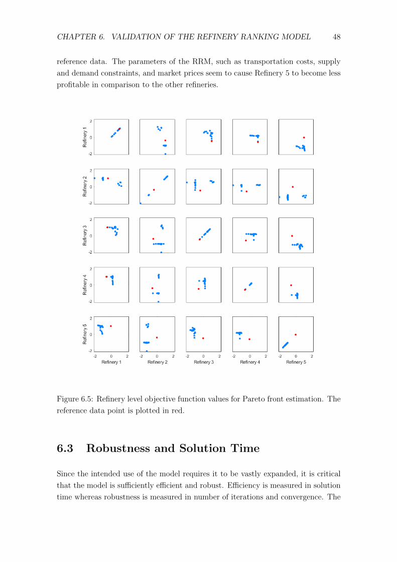
CHAPTER 6. VALIDATION OF THE REFINERY RANKING MODEL 48
reference data. The parameters of the RRM, such as transportation costs, supply
and demand constraints, and market prices seem to cause Refinery 5 to become less
profitable in comparison to the other refineries.
Figure 6.5: Refinery level objective function values for Pareto front estimation. The
reference data point is plotted in red.
6.3 Robustness and Solution Time
Since the intended use of the model requires it to be vastly expanded, it is critical
that the model is sufficiently efficient and robust. Efficiency is measured in solution
time whereas robustness is measured in number of iterations and convergence. The
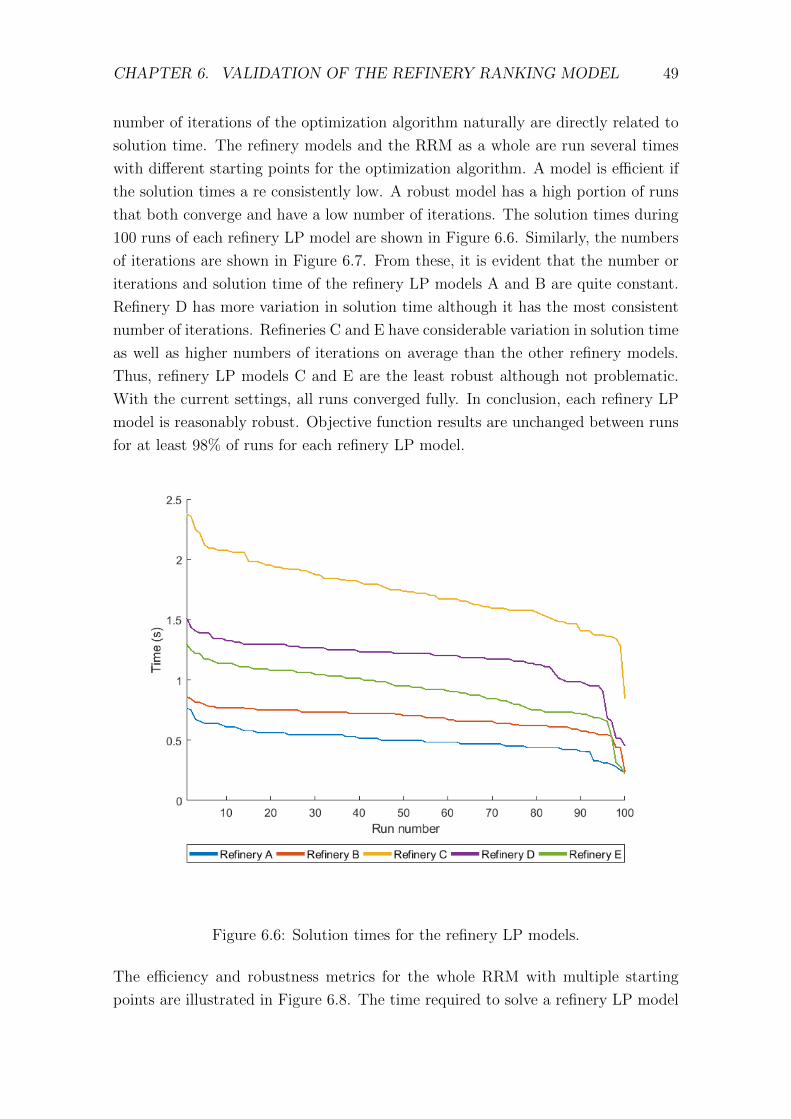
CHAPTER 6. VALIDATION OF THE REFINERY RANKING MODEL 49
number of iterations of the optimization algorithm naturally are directly related to
solution time. The refinery models and the RRM as a whole are run several times
with different starting points for the optimization algorithm. A model is efficient if
the solution times a re consistently low. A robust model has a high portion of runs
that both converge and have a low number of iterations. The solution times during
100 runs of each refinery LP model are shown in Figure 6.6. Similarly, the numbers
of iterations are shown in Figure 6.7. From these, it is evident that the number or
iterations and solution time of the refinery LP models A and B are quite constant.
Refinery D has more variation in solution time although it has the most consistent
number of iterations. Refineries C and E have considerable variation in solution time
as well as higher numbers of iterations on average than the other refinery models.
Thus, refinery LP models C and E are the least robust although not problematic.
With the current settings, all runs converged fully. In conclusion, each refinery LP
model is reasonably robust. Objective function results are unchanged between runs
for at least 98% of runs for each refinery LP model.
Figure 6.6: Solution times for the refinery LP models.
The efficiency and robustness metrics for the whole RRM with multiple starting
points are illustrated in Figure 6.8. The time required to solve a refinery LP model
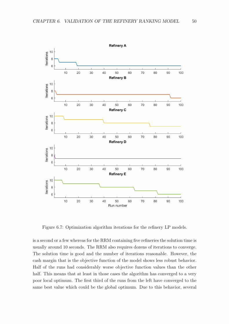
CHAPTER 6. VALIDATION OF THE REFINERY RANKING MODEL 50
Figure 6.7: Optimization algorithm iterations for the refinery LP models.
is a second or a few whereas for the RRM containing five refineries the solution time is
usually around 10 seconds. The RRM also requires dozens of iterations to converge.
The solution time is good and the number of iterations reasonable. However, the
cash margin that is the objective function of the model shows less robust behavior.
Half of the runs had considerably worse objective function values than the other
half. This means that at least in those cases the algorithm has converged to a very
poor local optimum. The first third of the runs from the left have converged to the
same best value which could be the global optimum. Due to this behavior, several
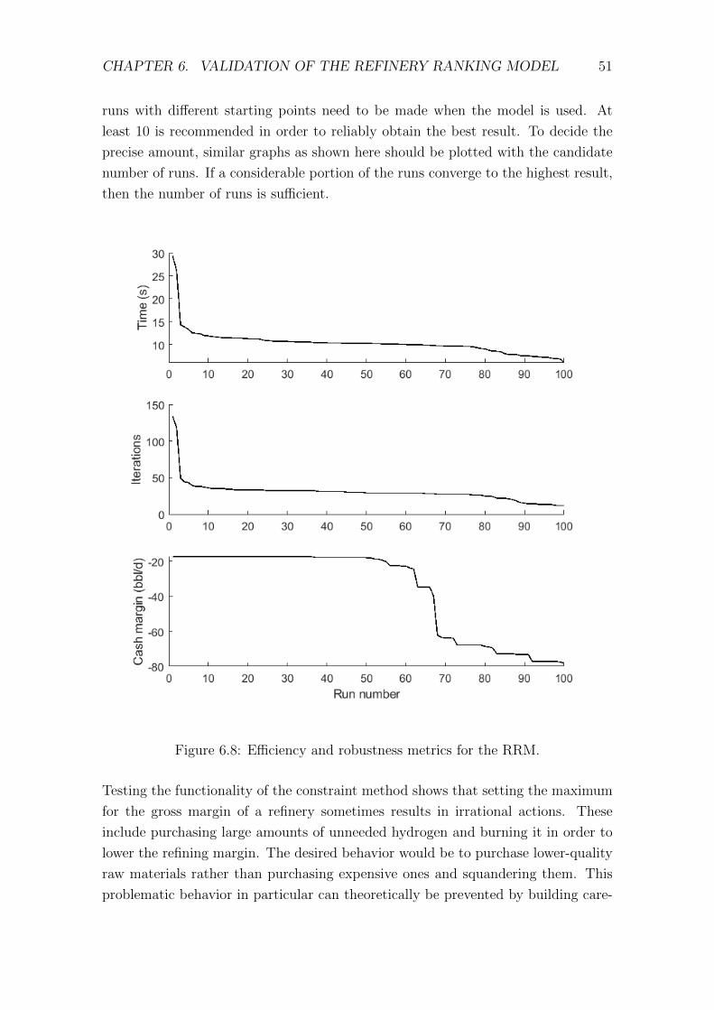
CHAPTER 6. VALIDATION OF THE REFINERY RANKING MODEL 51
runs with different starting points need to be made when the model is used. At
least 10 is recommended in order to reliably obtain the best result. To decide the
precise amount, similar graphs as shown here should be plotted with the candidate
number of runs. If a considerable portion of the runs converge to the highest result,
then the number of runs is sufficient.
Figure 6.8: Efficiency and robustness metrics for the RRM.
Testing the functionality of the constraint method shows that setting the maximum
for the gross margin of a refinery sometimes results in irrational actions. These
include purchasing large amounts of unneeded hydrogen and burning it in order to
lower the refining margin. The desired behavior would be to purchase lower-quality
raw materials rather than purchasing expensive ones and squandering them. This
problematic behavior in particular can theoretically be prevented by building care-

CHAPTER 6. VALIDATION OF THE REFINERY RANKING MODEL 52
ful constraints within the refinery models. Such safeguards are implemented in the
RRM to some degree. However, even if all such loopholes would be found adding
too many constraints like these could considerably increase the effort required to
correctly setup the model for a desired scenario. Thus, it is preferable to avoid set-
ting maximum limits to the objective functions of any subset of the model. If such
limits are put in place, it is recommended that they should not be much smaller than
the value that the unconstrained function would converge to. Unrealistic behavior
caused by the constraint method might be detected by comparison to results ob-
tained without the constraint method. With the constraint method, some decision
variables associated with very unprofitable decisions might have higher solution val-
ues. If more profitable decisions would be available without changing the decisions
of other refineries then it is likely that the constraint method is not yielding realistic
results for the scenario. If a constraint causes irrational behavior, then it should not
be used for the scenario.
In conclusion, the RRM model converges reliably and in reasonable time but the
individual objective functions exhibit unreliable behavior since they do not seem
to be directly related to the input parameters. A more extensive study should be
conducted before the model is taken into use or attempts are made to either expand
it or add detail. Also, use of the constraint method should be avoided.

Chapter 7
Market Price Sensitivity of Refin-
ing Margins
This chapter presents a sensitivity study using the Refinery Ranking Model (RRM)
built in this thesis. Generally, topics of interest include study of the conditions under
which the profitability order of different companies change, a competitor changes
their crude oil palette, or a refinery becomes unprofitable. The aim of this sensitivity
analysis is to test whether changes in the market scenario yield expected results.
Thus, a scenario should be selected such that the correct response to market change
can be confidently predicted. For example, all other things being equal, the increase
in all crude oil prices decreases the cash margin of all refineries. The sensitivity
of the refinery cash margins is tested by varying the prices of gasoline products
and crude oil. The market prices of the reference data are used as the median
for the analysis such that prices are varied below and above the reference values.
Neither the weighting method nor the constraint method are used in this sensitivity
analysis.
The effect of changes in gasoline products prices is displayed in Figure 7.1. Note
that the line illustrating the cash margins of all refineries is a weighted average
calculated from the cash margin and the volume throughput of each refinery. As
expected, the cash margins of each refinery tend to rise as the prices of the gasoline
products rise. However, between the point where the prices are altered -10 $/tonne
and the reference point there is a strong anomaly. The cash margins are lower
in the reference point than when the gasoline products prices are altered by -10
$/tonne. For a pure LP problem, the refining margins of all refineries should never
decrease when the price of a product increases. At most the refining margins of
some refineries could decrease and those of other refineries increase such that the
53
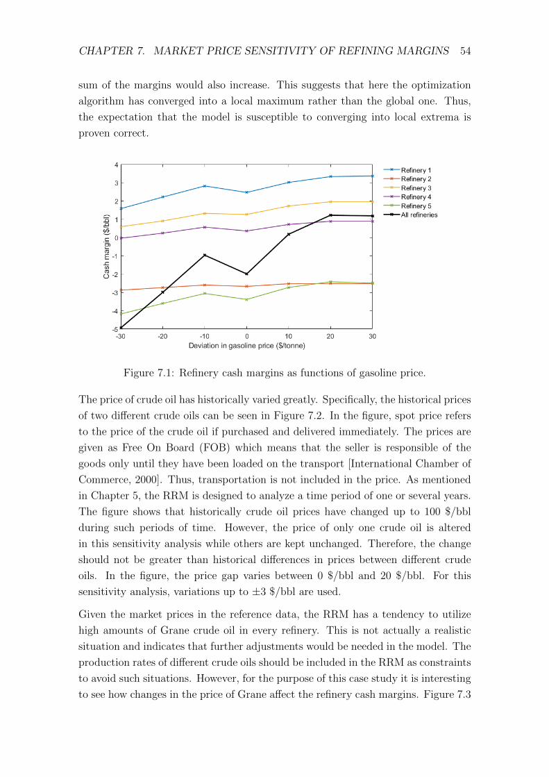
CHAPTER 7. MARKET PRICE SENSITIVITY OF REFINING MARGINS 54
sum of the margins would also increase. This suggests that here the optimization
algorithm has converged into a local maximum rather than the global one. Thus,
the expectation that the model is susceptible to converging into local extrema is
proven correct.
Figure 7.1: Refinery cash margins as functions of gasoline price.
The price of crude oil has historically varied greatly. Specifically, the historical prices
of two different crude oils can be seen in Figure 7.2. In the figure, spot price refers
to the price of the crude oil if purchased and delivered immediately. The prices are
given as Free On Board (FOB) which means that the seller is responsible of the
goods only until they have been loaded on the transport [International Chamber of
Commerce, 2000]. Thus, transportation is not included in the price. As mentioned
in Chapter 5, the RRM is designed to analyze a time period of one or several years.
The figure shows that historically crude oil prices have changed up to 100 $/bbl
during such periods of time. However, the price of only one crude oil is altered
in this sensitivity analysis while others are kept unchanged. Therefore, the change
should not be greater than historical differences in prices between different crude
oils. In the figure, the price gap varies between 0 $/bbl and 20 $/bbl. For this
sensitivity analysis, variations up to ±3 $/bbl are used.
Given the market prices in the reference data, the RRM has a tendency to utilize
high amounts of Grane crude oil in every refinery. This is not actually a realistic
situation and indicates that further adjustments would be needed in the model. The
production rates of different crude oils should be included in the RRM as constraints
to avoid such situations. However, for the purpose of this case study it is interesting
to see how changes in the price of Grane affect the refinery cash margins. Figure 7.3
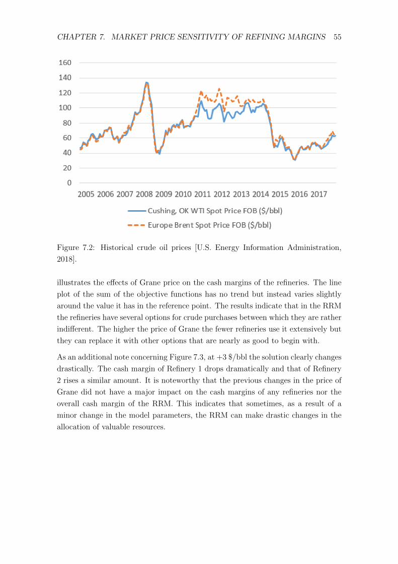
CHAPTER 7. MARKET PRICE SENSITIVITY OF REFINING MARGINS 55
Figure 7.2: Historical crude oil prices [U.S. Energy Information Administration,
2018].
illustrates the effects of Grane price on the cash margins of the refineries. The line
plot of the sum of the objective functions has no trend but instead varies slightly
around the value it has in the reference point. The results indicate that in the RRM
the refineries have several options for crude purchases between which they are rather
indifferent. The higher the price of Grane the fewer refineries use it extensively but
they can replace it with other options that are nearly as good to begin with.
As an additional note concerning Figure 7.3, at +3 $/bbl the solution clearly changes
drastically. The cash margin of Refinery 1 drops dramatically and that of Refinery
2 rises a similar amount. It is noteworthy that the previous changes in the price of
Grane did not have a major impact on the cash margins of any refineries nor the
overall cash margin of the RRM. This indicates that sometimes, as a result of a
minor change in the model parameters, the RRM can make drastic changes in the
allocation of valuable resources.
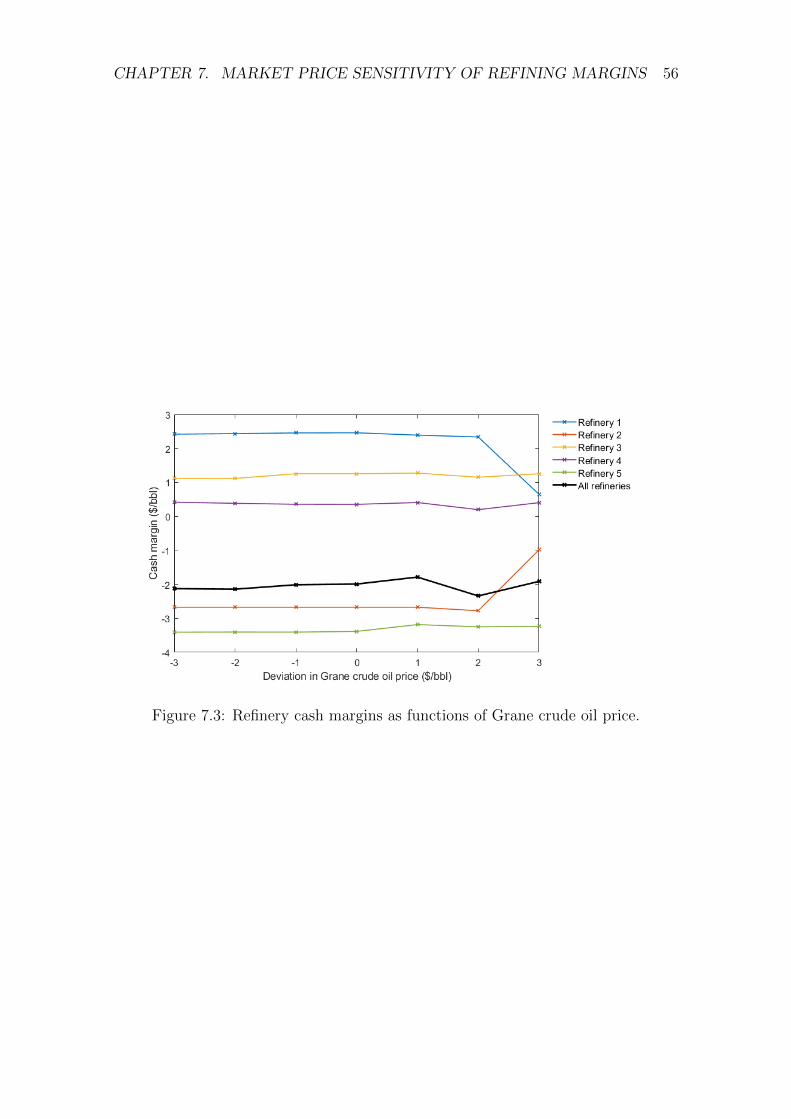
CHAPTER 7. MARKET PRICE SENSITIVITY OF REFINING MARGINS 56
Figure 7.3: Refinery cash margins as functions of Grane crude oil price.
Chapter 8
Discussion
This chapter discusses the challenges discovered in the earlier chapters as well as
potential pitfalls in future development of the RRM. Section 8.1 provides recommen-
dations for dealing with the undesirable behavior identified in the RRM in Chapters
6 and 7. In future development and use of the Refinery Ranking Model (RRM),
model complexity and the price parameters require attention. When the number
of refineries in the RRM is increased, it is imperative that robust solutions can be
obtained in reasonable time. Thus, the number of equations in the model must not
increase uncontrollably. An exponential increase in the number of equations is pos-
sible if model extensions are designed carelessly. This danger is addressed in Section
8.2. Also, a good understanding of the RRM requires a proper interpretation of the
price parameters. An arbitrary combination of price parameter values is not nec-
essarily realistic even if each parameter value is realistic on its own. The prices of
goods depend on supply and demand which, for some goods, the refining companies
could potentially affect. Section 8.3 explorers this phenomenon.
The case company has run several market scenarios where each price parameter is
specifically set for the scenario. These same scenarios should be run in the RRM
and the results compared to the existing ones. This could provide further insight
to the quality of both the RRM and the previous forecasting method. The RRM
is expected to outperform the older forecasting method especially in scenarios that
considerably differ from the reference data.
57
CHAPTER 8. DISCUSSION 58
8.1 Avoiding Undesired Behavior in the Refinery
Ranking Model
The results of the RRM often differ from the reference data. Potential causes of
deviation from the reference include differences in complexity and modeling solu-
tions, incomplete data, combining different data sources, averaging process data,
and differences in valuation of inter-refinery flows within companies.
In Chapter 7, two types of undesirable behavior were detected. First, convergence
to local optima was encountered. This was expected, as stated in Chapter 1. Sec-
ond, unpredictable allocation of resources among the refineries was detected. Small
changes in parameter values can have drastic effect on the operation of individual
refineries. For future applications of the RRM, it should be studied whether the
probability of such unpredictable and unrealistic solutions can be reduced. This
might be achieved through tighter constraints, more varied transportation prices
based on refinery location, or the utilization of the weighting method. Both types
of problematic behavior can be avoided to some degree by running the optimiza-
tion algorithm with several starting points as well as conducting sensitivity analysis.
The sensitivity of the solution of any scenario can be analyzed by altering the RRM
parameters. However, the number of parameters is high and sensitivity analysis for
the RRM is cumbersome. Therefore, only the most significant parameters can be
reasonably analyzed for most scenarios. The sensitivity analysis results can be used
to alter the parameters slightly in order to avoid a local optimum or a solution with
an unrealistic allocation of resources.
8.2 Model Complexity
Currently, the RRM comprises of five refinery nodes, five demand nodes, and a single
supply node which yield a grand total of 17 007 equations. There are 973 transport
links, 55 goods, 135 combinations of goods and locations for demands, as well as 30
combinations of goods and locations for supplies. In Europe there are around 80
refineries. Including all of those in the same manner as the model has been built so
far would result in the number of nodes increasing by a magnitude of ten or more.
The number of equations would increase exponentially. A rough estimation of the
number of equations ne is given as
CHAPTER 8. DISCUSSION 59
ne = kr(2500 + np · nS + ns · nD) + 1500 + C , (8.1)
where C is the number of additional case-by-case network-level constraints. In
the current RRM structure, C is small and directly proportionate to the number
of refineries. Thus, it is of no major concern. The constant 2500 is a result of
implementing one refinery LP model in more detail than the others. In Formula
8.1 it can be seen that, as more refineries are added, increasing also the number
of supply or demand nodes would lead to exponential increase in the number of
equations. Assuming 80 refineries, 80 demand nodes, and a single supply node the
theoretical number of equations would be more than one million.
Since using and updating the model requires labor it is not realistic to assume such
a huge amount of equations could be handled with reasonable effort and acceptable
risk of human error. Luckily, when more refineries are added, a notable portion of
the equations will be redundant because often faraway clients are not viable to a
given refinery. By identifying the redundant connections between nodes it is possible
to divide the model into market regions. These would likely compete for the same
crude oil supply but sell their products to different markets. Therefore, by carefully
selecting which nodes are connected to each other, the RRM could be built such
that the number of equations approximately follows the following formula
ne = kr(2500 + np · n′S + ns · n′D) + 1500 + C , (8.2)
where n′S, and n′D are the numbers of supply and demand nodes, respectively, in a
single market region only. It is assumed that these figures are roughly the same for
each market region. Assuming that each market region contains 10 refineries, every
additional 10 refineries increase the number of equations by an amount equal to the
toal number of equations in a model that includes only the first 10 refineries.
In case there is need to further limit the number of equations, the model structure
needs to be altered considerably. Three alterations are suggested. Firstly, refineries
could be classified such that a smaller number of different refinery topologies would
need to be implemented and maintained. Secondly, refineries that have a lesser
market impact on the case company could be depicted such that all refineries of
a company are represented as a single refinery with increased capacity. Thirdly,
markets that have a lesser impact on the case company could be described with less
detail such that the markets of several countries would be pooled together into a
single demand node and a supply node if necessary.

CHAPTER 8. DISCUSSION 60
8.3 Price Parameters and Game Theory
Any set of price parameters used in the model depicts some market equilibrium.
This equilibrium can be selected based on historical observations, predictions of the
future, or simply curiosity towards otherwise interesting scenarios. In practice, such
an equilibrium is reached as the result of the actions taken by all the agents that can
affect the industry. These agents include several petroleum exploration companies,
petroleum refineries, end-customers, and policymakers. However, subsets of these
agents can be identified and their behavior potentially understood and predicted
with enough precision to gain some understanding of the dynamics that form the
market equilibrium. For example, an attempt could be made to understand the
behavior of the refining companies by describing their mutual competition as a
game. Such an analysis might provide further understanding on whether a selected
set of prices or some solution given by the RRM is feasible.
A problem with the RRM introduced in this thesis is that some scarce supplies
might be excessively allocated to a certain refinery even if in reality others would
compete for it as well. This kind of a situation was shown in Chapter 7. In such
situations, assuming perfect competition, the price of the good would rise to the
highest level that any refinery would be willing to pay. That price would then
match the true market equilibrium price. It is noteworthy that the refinery willing
to pay the final price might not be the same as the refinery that the resource is
currently allocated to in the RRM. This shows how the price parameters selected
for the model can sometimes be poorly selected but it is not easy to detect whether
that is the case.
An attempt to simulate such market reactions could be made by running the model
repeatedly with the analyzed price increased by a step for each run. The refinery
that the scarce good is originally allocated to should be inactive for the duration of
the test. Once the price would reach a level where that good is no longer allocated
or it is allocated to a very poor option, the inactive demand could be reactivated.
If the good would still be allocated to that demand it would indicate that this is
the price that only this particular refinery is willing to pay for that good. However,
this is problematic since the model dynamics are affected by the inactivation of that
particular refinery. A solution to this might be to increase the supplied amount of
the good to be analyzed and then increase the price to find the point where there
remains only one refinery that is willing to pay for the good. Of course, there could
be several reasons for some refinery to obtain certain goods for a better price than
others. The transportation costs of the RRM are used to account for such situations
CHAPTER 8. DISCUSSION 61
where the price of a good is different for different refineries.
As briefly discussed in Chapter 2, describing the system of the RRM additionally
as a cooperative game could be used to explore the best possible refining margins
attainable by the refineries should they choose to cooperate. Although the coop-
erative situation itself is unrealistic, its results could be compared to those of the
RRM to better understand the MOLP model. The realistic allocation of resource
in the RRM proved problematic due to the inherent difficulty of strictly specifying
competition in a MOLP model. When using the weighting method or no scalariza-
tion method at all the optimization algorithm sees the RRM as a cooperative model
with transferable utility. It only maximizes the total refining margin of the system
as a whole. Although some ideas are represented for encouraging the RRM towards
realistic behavior, it is not easy to judge the results given limited reference data.
Thus, comparison with both a competitive and a cooperative game theoretic model
could be used to analyze how close the RRM solutions are to either cooperation or
competition.
Chapter 9
Conclusions
In this thesis, a competition situation of multiple refining companies was formulated
as a multi-objective linear programming problem. A practical implementation of the
problem was introduced and labeled the Refinery Ranking Model (RRM). It ranks
the profitability of competing petroleum refineries under different market scenarios.
The solution of the RRM provides detailed values of the purchases, sales, operating
costs, and operating parameters of the different refineries. Although the model
is formulated as a optimization model the main practical use is simulations that
identify the impact of different market scenarios. The most intuitive use of the
RRM is to simulate the relative and absolute profitability of refineries in different
market situations. Another beneficial simulation study is to explore the effect of
market prices on the behavior of competitors. This can help understand, e.g, when
a competitor will change from one crude oil to another. A third basic use for the
RRM is running a sanity check for extreme scenarios before applying them to other
analysis. For example, if a majority of refineries in the RRM become unprofitable in
a given market scenario then the scenario might be overly pessimistic. The RRM is
developed for the Finnish oil refining and renewable solutions company Neste using
Spiral Suite1 optimization software.
The RRM consists of several refinery models linked together into a network. Each
refinery affects their competitors as well as having synergy benefits with other re-
fineries owned by the same refining company. The greatest challenge in utilizing
multi-objective linear programming for such a competition situation is obtaining
results where each refinery aims to maximize the profit of its own company rather
than the total profit of all companies. In order to find the desired Pareto-optimal
solutions using the Spiral Suite1 software, the weighting method and the constraint
method were explored. Under certain circumstances, the constraint method can
1 Spiral Suite by AVEVATM
CHAPTER 9. CONCLUSIONS 63
yield very unrealistic results even if realistic constraints and parameters are used.
In these cases, the profits of some refineries are brought down artificially to circum-
vent some constraints and increase the total profit in the model. Thus, the use of the
constraint method is not recommended. The weighting method is more robust and
is successfully used to emphasize the importance of some refineries over others.
The refineries in the RRM are single-objective LP models. Each refinery model is
built of the same process model units although configurations differ. This reduces
the burden of maintenance when changes are made to the RRM in order to expand
or update it. The refineries’ product palettes and profitability were compared to
reference data and some deviations were found. However, potential causes for these
deviations were identified and they can be eliminated in future development.
To validate the results of the RRM, they were compared to existing reference data.
Furthermore, the RRM’s sensitivity to some market price parameters was tested
and the feasibility of the results evaluated. Analysis on the results of the RRM
revealed that there are local maxima into which the model can converge. This
was expected due to the nonlinear nature of some of the refining processes in the
RRM. It was also discovered that the model sometimes allocates scarce resources
unrealistically such that the competition situation becomes skewed. Revising the
constraints and geographical impact or using the weighting method are suggested
as possible solutions.
Since there are over 80 refineries in Europe alone, the RRM is currently very con-
stricted and as such does not reflect the wider dynamics of the industry. Future
development would likely include adding further refinery models and possibly ad-
justing the level of detail in both markets and refineries. Other market areas such as
Asian and American markets, including their refineries, would be sensible to describe
simply as large supply and demand nodes with their parameters and transport links
set accordingly. A similar approach could be taken also with regions within Europe
to reduce solution time as well as effort in implementation, maintenance, and usage.
The trade-off in this approach is the loss of detail in the model.
There are two major issues in the RRM design. The first one is the quality of the
reference data. The data is at times incomplete or outdated. Also, since several
data sources are used it is questionable whether the data from different sources
matches the same market and refinery operating conditions. The second issue is
the competition dynamics of the refining companies. The selection between Pareto-
optimal solutions would benefit from further market and technical insight. If the
RRM is expanded to include dozens of refineries, then the task of selecting the so-
lution becomes even more difficult. Therefore, an iterative method is recommended
CHAPTER 9. CONCLUSIONS 64
for finding the realistic options among the Pareto-optimal solutions.
In conclusion, the RRM can be utilized for several useful simulations. These sim-
ulations can assist in planning company strategy and increase understanding of
competitors’ potential actions. The RRM can be expanded to cover large systems
of refineries with reasonable increase in solution time. Expanding and maintaining
the RRM requires low effort since all of the refinery models are constructed of the
same process unit models.
Bibliography
M. A. Al-Sahlawi. Structure of the oil and gas industry. In K. A. Hussein and M. A.
Al-Sahlawi, editors, Petroleum Economics and Engineering, chapter 2, pages 21–
40. Taylor & Francis Group, Boca Raton, Florida, 2014. ISBN 978-1-4665-066-4.
C. A. Bana e Costa. Readings in Multiple Criteria Decision Aid. Springer-Verlag
Berlin, Heidelberg, Germany, 1990. ISBN 978-3-642-75935-2.
E. N. Barron. Game theory: An Introduction. Wiley, NY, 2013. ISBN 978-1-118-
21693-4.
BBC. Internet website, 2017. URL http://www.bbc.co.uk/education/guides/
zm2v4wx/revision. Accessed 15.9.2017.
N. Bret-Rouzaut and J.-P. Favennec. Oil and Gas Exploration and Production:
Reserves, Costs, Contracts. Editions Technip, Paris, France, 2011. ISBN 978-1-
62198-679-9.
M. A. Fahim, T. A. Alsahhaf, and A. S. Elkilani. Fundamentals of Petroleum
Refining. Elsevier, Amsterdam, Netherlands, 2010. ISBN 9780080931562.
F. R. Fernandez, M. G. Fiestras-Janeiro, I. Garcıa-Jurado, and J. Puerto. Com-
petition and cooperation in non-centralized linear production games. Annals of
Operations Research, Volume 137(1):91–100, 2005. ISSN 1572-9338.
B. Fleischmann, H. Meyr, and M. Wagner. Advanced planning. In H. Stadtler,
C. Kilger, and H. Meyr, editors, Supply Chain Management and Advanced Plan-
ning, chapter 4, pages 71–95. Springer, Berlin, 2015. ISBN 978-3-642-55309-7.
S. Flam, G. Owen, and M. Saboya. The not-quite non-atomic game: Non-emptiness
of the core in large production games. Mathematical Programming, Volume 9(1):
358–370, 1975. doi: 10.1007/BF01681356.
B. Friedland. Control System Design : An Introduction to State-space Methods.
Dover Publications, Mineola, NY, 1986. ISBN 0-486-44278-0.
65
BIBLIOGRAPHY 66
K. Hastbacka, H. Haapalinna, P. Herring, and H. Manninen. Neste - From Oil to
Plastics. Neste Oy, Espoo, Finland, 1993. ISBN 952-9553-06-4.
International Chamber of Commerce. Preamble, FOB, 2000. URL
https://web.archive.org/web/20030417131953/http://www.iccwbo.org/
incoterms/preambles/pdf/FOB.pdf. Accessed 12.5.2017.
P. S. H. Leeflang. Modeling competitive reaction effects. Schmalenbach Business
Review, Volume 60(4):322–358, 2008. ISSN 2194-072X.
P. S. H. Leeflang, J. E. Wieringa, T. H. Bijmolt, and K. H. Pauwels. Advanced
Methods for Modeling Markets. Springer International Publishing, Philadelphia,
PA, USA, 2017. doi: 10.1007/978-3-319-53469-5.
W. L. Leffler. Petroleum Refining in Nontechnical Language. PennWell cop., Tulsa,
Oklahoma, USA, 2008. ISBN 978-1-62198-760-4.
T. Lenahan. Turnaround, Shutdown and Outage Management : Effective Plan-
ning and Step-by-step Execution of Planned Maintenance Operations. Elsevier,
Burlington, MA, 2006. ISBN 978-0-08-052527-3.
K. Miettinen. Nonlinear Multiobjective Optimization. Kluwer Academic Publishers,
Boston, MA, 1999. ISBN 0-7923-8278-1.
Ministry of Economic Affairs and Employment, Finland. Security of Energy Supply,
2018. URL http://tem.fi/en/security-of-energy-supply. Accessed 14.5.2017.
National Institute of Standards and Technology, U.S. Department of Commerce.
Guide for the Use of the International System of Units (SI), 2008. URL https://
nvlpubs.nist.gov/nistpubs/Legacy/SP/nistspecialpublication811e2008.pdf.
Accessed 14.5.2017.
S. M. S. Neiro and J. M. Pinto. A general modeling framework for the operational
planning of petroleum supply chains. Computers & Chemical Engineering, Volume
28(6-7):871–896, 2004. doi: 10.1016.
Neste. Internet website, 2017. URL https://www.neste.com/en. Accessed 15.9.2017.
S. Parkash. Refining Processes Handbook. Elsevier, Amsterdam, Netherlands, 2003.
ISBN 978-0-08-052385-9.
M. R. Riazi. Characterization and Properties of Petroleum Fractions. American
Society for Testing and Materials, West Conshohocken, PA, 2005. ISBN 0-8031-
3361-8.
BIBLIOGRAPHY 67
M. Sakawa, H. Yano, and I. Nishizaki. Linear and Multiobjective Programming with
Fuzzy Stochastic Extensions. Springer US, Boston, MA, 2013. ISBN 978-1-4614-
9399-0.
J. G. Speight. An Introduction to Petroleum Technology, Economics, and Politics.
Wiley, Salem, MS; Hoboken, NJ, 2011. ISBN 9781118192559.
Statistics Finland. Energy prices: 3rd Quarter 2017, Appendix figure 1, Import
prices of oil, 2017. ISSN 1799-800X. URL http://www.stat.fi/til/ehi/2017/
03/ehi_2017_03_2017-12-07_kuv_001_en.html. Accessed 21.12.2017.
G. H. Symonds. Linear Programming: The Solution of Refinery Problems. Esso
Standard Oil, New York, 1955.
U.S. Energy Information Administration. Petroleum and Other Liquids Data, 2018.
URL https://www.eia.gov/. Accessed 12.5.2017.
M. Yoshimi, T. Kuhara, K. Nishimoto, M. Miki, and T. Hiroyasu. Visualization of
pareto solutions by spherical self-organizing map and it’s acceleration on a gpu.
Journal of Software Engineering and Applications, Volume 5(3):10, 2012. doi:
10.4236.