75

A Multi-level Iterative Linear Solver for Circuit Simulation

Reiji Suda (須田礼仁)

Dept. Information Science, The University of Tokyo

1. Introduction

Circuit simulation is an indispensable tool for circuit design. It is the only way to pre-

estimating and optimizing $IC/LSI$ circuits, for which ‘trial-and-error’ is too costly. Circuit

simulat\‘ion is used for verification of circuit design as well, in conjunction with translators

from chip layout to circuit model. The speed of micro computers grows faster, and circuit

simulation begins to be used for board level design. Up to circuits with a few tens of

thousand nodes can be simulated in the current technology, but still faster simulators are

expected for simulation of higher precision, longer time, and larger circuits.

The modelization of circuit simulation is well founded [1]. Fundamental equations

are the Kirchhoff’s voltage and current laws combined with current-voltage relationship

of elements. Differential and integral on time appear for capacitors and inductors, and

the equations are ordinary-differential equations, which are transformed into a series of

non-linear equations at each time steps by a stiff-stable numerical integral algorithm such

as the backward Euler method and the Gear methods. Each set of non-linear equations is

usually solved by Newton-Raphson method, where linear equations are repeatedly solved.

Linear equations in the Newton iteration are highly sparse: The average non-zero ele-

ments per row is typically less than ten, while the size of matrix can be several thousand.

However preferable properties for iterative linear solvers–simple banded structure, sym-

metry, M-matrix, or positive definiteness –are not hold in many cases. Therefore with

few exceptions which considers iterative methods $[2][3][4]$ , direct methods such as LU-

decomposition with Markovitz-Tewarson’s fill-in minimization [5] and the code generation

method [6] are employed.

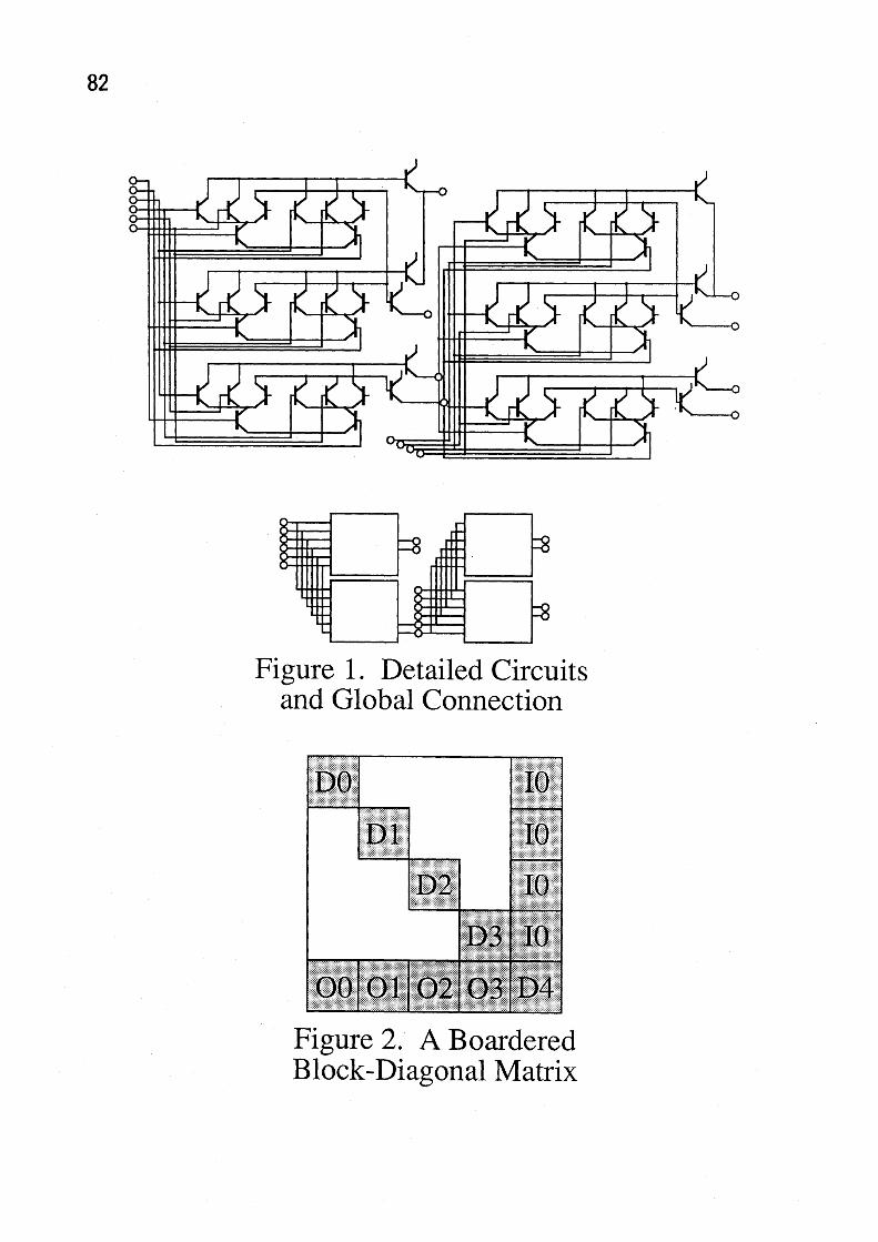
This paper tries to introduce the multi-grid method, which has succeeded on wide

area of applications, onto the circuit simulation, choosing the detailed circuit model as the

‘fine grid’ and connection between gates as the ‘coarse grid’ (Figure 1). Main difficulties on

数理解析研究所講究録第 832巻 1993年 75-85

76

employment of the multi-grid concepts for circuit simulation are the random structure and

the high non-linearity, which enforces complicated and dynamic computation of translation

(restriction and prolongation) matrices. The proposed algorithm shows closer relation with

direct methods than other multi-grid algorithms, but is actually an iterative solver using

approximated problems. It is implemented in a Josephson junction circuit simulator, and

reduces time for linear solution into 2/3 of the LU decomposition. Although it is not tested

for semiconductor circuits, but will effective especially in memory and CMOS circuits.

2. Block LU Decomposition and Multi-level Iteration

Circuits in circuit simulators are defined as a set of subcircuits and connections be-

tween them. The corresponding matrix structure is a bordered block-diagonal (Figure

2)[7], where off-border diagonal blocks $(D_{i}’ s)$ correspond with gates, and border diagonal

block $(D_{n})$ corresponds with the global network. The diagonal blocks are assumed to be

reversible (and therefore square), since otherwise linearly dependent rows and columns can

be purged into the border part. Then the LU decomposition of the i-th block can choose

pivots within the i-th diagonal block $(D_{i})$ , and touches only the i-th upper/lower border

blocks ( $I_{i}$ and $O_{i}$ in Figure 1), the border diagonal block $(D_{n})$ , and the i-th diagonal block

itself $(D_{i})$ . Therefore each subblock is decomposed independently up to the size of the

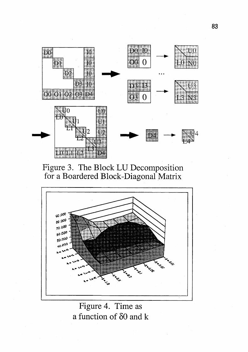
diagonal block as:$(\begin{array}{ll}D_{i} LO_{i} 0\end{array})=L_{i}N_{i}U_{i}$ (1)

then residual parts $(N_{i}’ s)$ are accumulated into the last diagonal block (Figure 3), which

is then decomposed into $L_{n}U_{n}$ .

Assuming that good approximations for $L_{i}’ s,$ $N_{i}’ s$ , and $U_{i}’ s$ are known (denote them$\tilde{L}_{i},\tilde{N}_{i}$ , and $\tilde{U}_{i}$ ), the LU decomposition process is reduced into accumulation of $\tilde{N}_{i}’ s$ into$D_{n}$ and LU decomposition of the resultant small matrix. The relaxation-like iteration can

be applied to improve precision:

$x$ $:=x+\tilde{A}^{-1}(b-Ax)$ (2)

where $\tilde{A}^{-1}=\tilde{U}^{-1}\tilde{N}^{-1}\tilde{L}^{-1}$ represents the substitution process of the approximately LU-

decomposed matrix. This process can be viewed as a coarse grid correction where $\tilde{L}^{-1}$

77

is the restriction, $\tilde{N}^{-1}$ is the solution on coarse grid ( $=$ global network), and $\tilde{U}^{-1}$ is

the prolongation. Much time will be saved when $\tilde{L}$ and $\tilde{U}$ can be fixed with reasonable

approximation precision (which looks usual in other multi-grid methods), but experiments

shows that on-line computation of $\tilde{L}$ and $\tilde{U}$ is unavoidable for highly non-linear circuits.

The required precision on $\tilde{A}=\tilde{L}\tilde{U}$ is estimated next.

The linear solver is used only in the Newton iteration, and therefore higher precision

than the Newton iteration is a waste of computation. Assume that $\frac{||b-Ax||}{||b||}\leq\epsilon$ is

required ( $||$ . I denotes a consistent norm of vector and matrix), and that the initial $x$ is a

zero vector. After $n$ times iteration, the residue becomes

$b-Ax^{(n)}=(I-\tilde{A}^{-1}A)^{n}b$

(3)$=A^{-1}(E\tilde{A}^{-1})^{n}Ab$

where $E=\tilde{A}-A$ . The requirement is satisfied when

$(||E\tilde{A}^{-1}||)^{n}\leq\epsilon$ (4)

from which$( \kappa(A)\frac{||E||}{||A||})^{n}\leq\epsilon$ (5)

is obtained, where $||\tilde{A}||$ and $\kappa(\tilde{A})$ are approximated with $||A||$ and $\kappa(A)$ . Therefore the

required approximation precision is:

$\frac{||\tilde{A}-A||}{||A||}\leq(\frac{\epsilon}{\kappa(A)})^{1/n}$ (6)

3. Implementation of Multi-level Circuit Simulation

Approximation scheme

One method to get $\tilde{L}^{-1}$ and $\tilde{U}^{-1}$ is use of decompositions of some steps before while

they are precise enough, and re-decompose local matrices when the precision condition

discussed in the previous section breaks. In this method, the precision of the approximation

depends on the condition of re-decomposition, and can be controlled dynamically through

setting of the referred precision $\epsilon$ . A special case of this scheme is the conventional direct

78

method in which all submatrices are decomposed in every Newton iteration. This method

is expected to be effective where only a small part of gates are dynamic and need re-

decomposition of the matrices. It will more effective in clocked digital circuits rather

than analog circuits, and the most hopeful target is static memories where non-selected

memory cells are completely static. Another hope is CMOS circuits: The power dissipation

of CMOS circuits is proportional to the state switch. Therefore a good CMOS design will

minimize the frequency of state switch, which will reduce frequency of re-decomposition

of matrices in this algorithm.

Another approximation method is pre-computation: Compute a set of approximated

decompositions from which a decomposition with enough precision can be chosen for any

possible realization of the matrix. This scheme may be viewed as an extension of tabled

elements for user-defined subcircuits, or an introduction of logic simulation concepts where

gates have only discrete states. Two problems are to be solved: (1) how to make a precise

enough set of decompositions, and (2) how to select a decomposition from the prepared

set. Another problem is memory consumption for a large set of decomposition results (but

one set is enough for gates of the same definitions). However, the simulation is completely

free from local decompositions.

Implementation

The multi-level iteration algorithm is implemented in Josephson junction circuit sim-

ulator, where decomposition of some steps before is used as an approximation matrix.

Resumumption of re-decomposition is based on Eq. (6), where $||A||$ is computed once be-

fore the simulation, and $\kappa(A)$ is replaced by a manually defined value. On line calculation

of $\kappa(A)$ or even $||A||$ is costly, and high precision is not indispensable for these parameters

since another parameter $\epsilon$ , which is the resultant residue of Newton iteration, cannot be

precise. The linear solver algorithm is as follows:

$/*$ Approximated LU decomposition $*/$

Predict Newton iteration’s relative precision $\epsilon$

If $(\delta_{0}\geq\sqrt{\epsilon k})$ then

Let $n=2$ and $\delta=\sqrt{\epsilon k}$

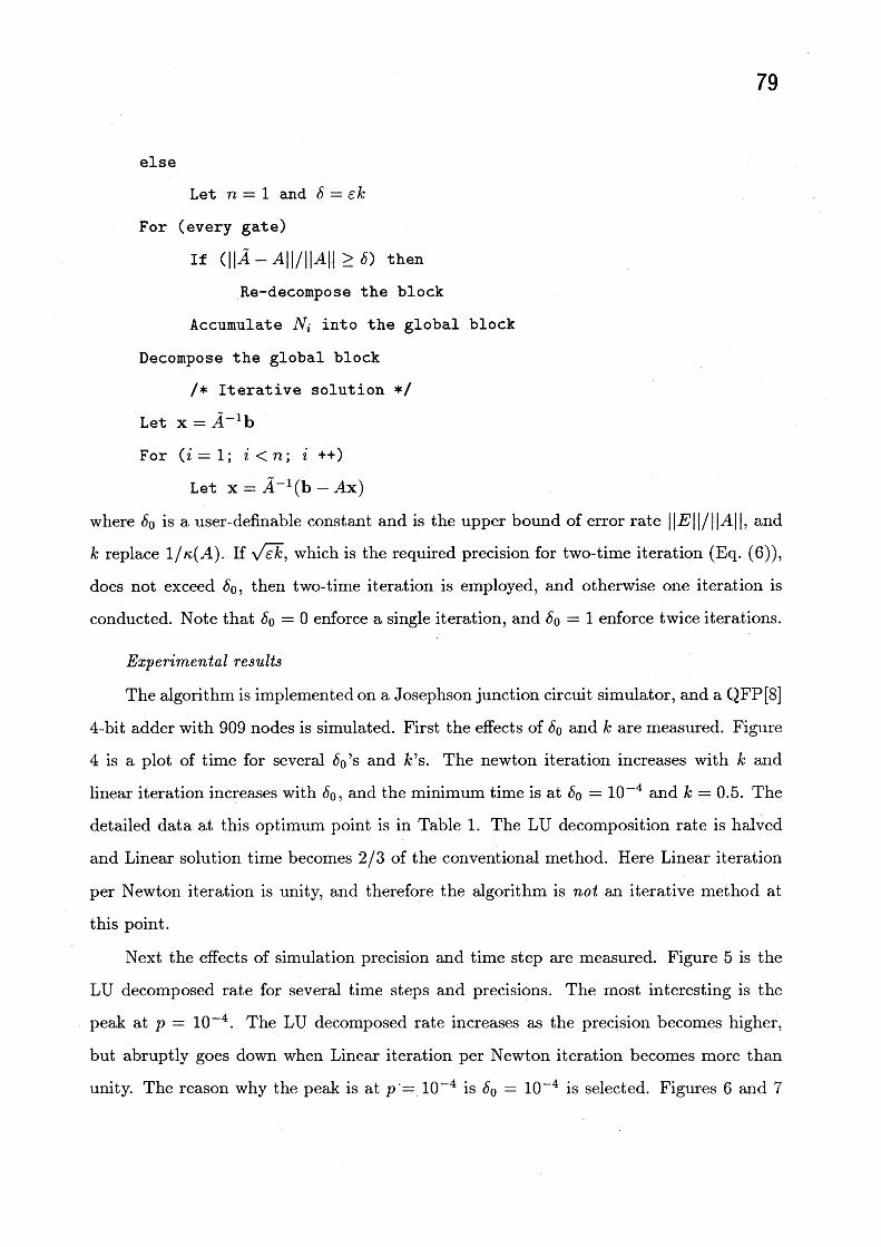
79

else

Let $n=1$ and $\delta=\epsilon k$

For (every gate)

If $(||\tilde{A}-A||/||A||\geq\delta)$ then

Re-decompose the block

Accumulate $N_{i}$ into the global block

Decompose the global block

$/*$ Iterative solution $*/$

Let $x=\tilde{A}^{-1}b$

For $(i=1;i<n;i++)$Let $x=\tilde{A}^{-1}(b-Ax)$

where $\delta_{0}$ is a user-definable constant and is the upper bound of error rate $||E||/||A||$ , and

$k$ replace $1/\kappa(A)$ . If $\sqrt{\epsilon k}$, which is the required precision for two-time iteration (Eq. (6)),

does not exceed $\delta_{0}$ , then two-time iteration is employed, and otherwise one iteration is

conducted. Note that $\delta_{0}=0$ enforce a single iteration, and $\delta_{0}=1$ enforce twice iterations.

Experimental results

The algorithm is implemented on a Josephson junction circuit simulator, and a QFP [8]

4-bit adder with 909 nodes is simulated. First the effects of $\delta_{0}$ and $k$ are measured. Figure

4 is a plot of time for several $\delta_{0}’ s$ and $k’ s$ . The newton iteration increases with $k$ and

linear iteration increases with $\delta_{0}$ , and the minimum time is at $\delta_{0}=10^{-4}$ and $k=0.5$ . The

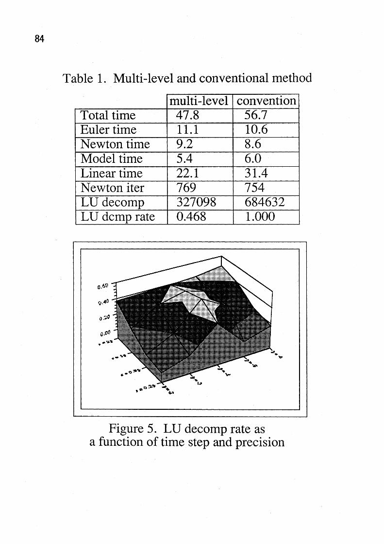
detailed data at this optimum point is in Table 1. The LU decomposition rate is halved

and Linear solution time becomes 2/3 of the conventional method. Here Linear iteration

per Newton iteration is unity, and therefore the algorithm is not an iterative method at

this point.

Next the effects of simulation precision and time step are measured. Figure 5 is the

LU decomposed rate for several time steps and precisions. The most interesting is the

peak at $p=10^{-4}$ . The LU decomposed rate increases as the precision becomes higher,

but abruptly goes down when Linear iteration per Newton iteration becomes more than

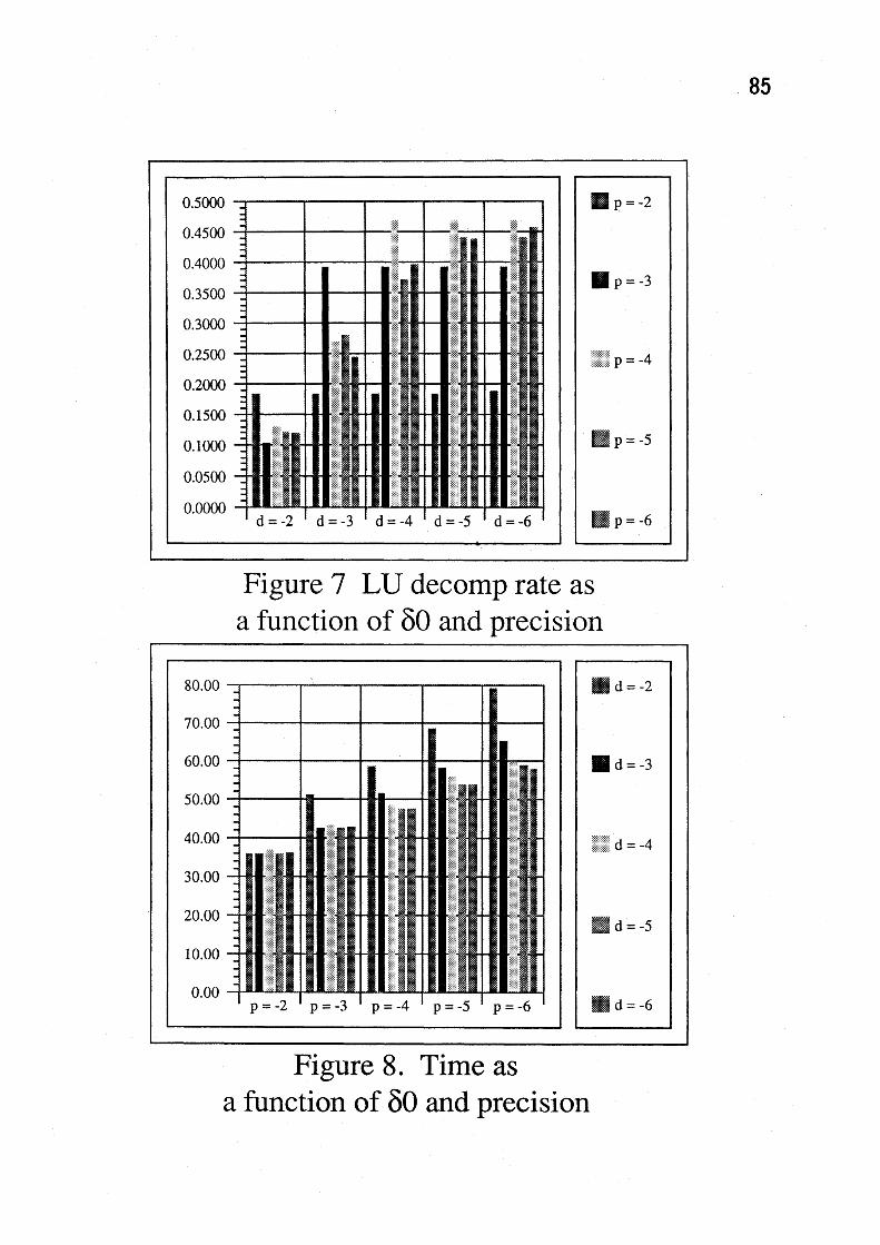
unity. The reason why the peak is at $p’=10^{-4}$ is $\delta_{0}=10^{-4}$ is selected. Figures 6 and 7

80

prove that the LU decomposition peaks appear at $p\approx\delta_{0}$ , which give the minimum time

at the same time.

The following facts are founded through the above experiments: (1) $\delta_{0}$ should be same

as the simulation precision or smaller, where LU decomposition rate is maximized and no

more than one Linear iteration is conducted per Newton iteration. (2) 0.5 for $k$ has been

the best. Larger $k$ reduces LU decomposition rate, but 1.0 is too large. The potimum

parameter has reduced the linear solution time into 2/3 of the conventional method.

4. Conclusion

This paper introduces the multi-level iteration concepts into circuit simulation. The

coefficient matrix in circuit simulation is bordered block-diagonal, where diagonal blocks

correspond with gates and border diagonal block corresponds with global connection. Lin-

ear equation is solved by iteration with approximated matrices which were precise matrices

of some steps before. This scheme is effective when only a part of gates shift their states

rapidly, and such situation is expected especially in memory and CMOS circuits. The

proposed algorithm has been implemented in a Josephson junction circuit simulator, and

has reduced linear solution time into 2/3 of the conventional LU decomposition. Future

works are application to semiconductor circuits, implementation of other approximation

schemes, and extension of the multi-level concepts into the levels of non-linear equations

and ordinaly-differential equations.

References

[1] L. W. Nagel, “SPICE 2–A Computer Program to Simulate Semiconductor Cir-

cuits,” Univ. of California, Berkley, ERL Memo, ERL-M 520, May 1975.

[2] A. R. Newton and A. L. Sangivanni-Vincentelli, “Relaxation-Based Electrical Sim-

ulation,” IEEE Trans. CAD, Vol. 3, No. 4, pp. 308-331, Oct., 1984.

[3] F. Yamamoto, Y. Umetani, S. Takahashi, “Applicability of Conjugate Residue with

Complete LU decomposition for Large-Scale Circuit simulation,” Trans. IPSJ,

Vol. 27, No. 8, Aug. 1986, pp. 774-782 (in Japanese).

81

[4] R. Suda and Y. Oyanagi, “Josephson junction Circuit Simulation with Precondi-

tioned Gauss-Seidel Method,” IPSJ SIG notes, Vol. 92, No.66, Aug. 1992, pp. 1-8

(in Japanese).

[5] R. P. Tewarson, Sparse Matrices, Academic Press, 1973.

[6] F. G. Gustavson, W. Liniger, and R. A. Willoughby, “Symbolic Generation of an

Optimal Crout Algorithm for Sparce Systems of Linear Equations,” JACM, Vol. 17,

No. 1, Jan., 1970, pp. 87-109.

[7] G. D. Hachtel and A. L. Sangiovanni-Vincentelli, “A Survey of Third-Generation

Simulation Techniques,” Proc. IEEE, Vol. 69, No. 10, Oct. 1981, pp. 1264-1280.

[8] W. Hioe and E. Goto, Quantum Flux Parametron, Singapore: World Scientific,

1991.

82

Figure 1. Detailed Circuitsand Global Connection

Figure $2_{:}$ A BoarderedBlock-Diagonal Matrix

83

$arrow$

$arrow$

–

Figure 3. The Block LU Decompositionfor a Boardered Block-Diagonal Matrix

a function of 60 and $k$

84

Table 1. Multi-level and conventional method

Figure 5. LU decomp rate asa function of time step and precision

85

Figure 7 LU decomp rate as

Figure 8. Time asa function of 60 and precision