A multi-criteria approach to robust outsourcing decision-making in stochastic manufacturing systems Hahn G, Sens T, Decouttere C, Vandaele N.

KBI_1421

A multi-criteria approach to robust outsourcing decision-making

in stochastic manufacturing systems

G. J. Hahna∗∗, T. Sensa, C. Decouttereb and N. VandaelebaUniversity of Mannheim, Germany; bKatholieke Universiteit Leuven, Belgium

October 9, 2014

Abstract

Manufacturing outsourcing is a key industry trend towards greater operational efficiency and isrelated to the discussion of strategic core competencies. We study the issue of contract manufac-turing at the strategic-tactical level and approach the topic from a multi-criteria decision-makingperspective, since service, cost, quality, and more long-term value-related aspects are involved.To arrive at well-balanced and robust outsourcing decisions with respect to the aforementioneddimensions, we apply a scenario-based approach that is built within the concept of Data Envelop-ment Analysis (DEA). For this purpose, we use two types of Key Performance Indicators (KPIs):model-based KPIs, which are the result of a modeling approach, and non-model-based KPIs thatare derived in an independent assessment from multiple stakeholders. The model-based KPIs arehandled through an aggregate planning model which manages the trade-off of capacity vs. work-in-process costs and uses a queuing network-based approach to anticipate the stochastic and dynamicbehavior of a manufacturing system. This allows us to balance customer service, derived from ag-gregate order lead times, and relevant costs of operations when determining volume/mix decisionsfor internal and external production. An industry-derived case example with distinct outsourcingoptions is used to highlight the benefits of the approach.Keywords: Multi-criteria decision-making, stochastic models, outsourcing, manufacturing sys-tems, aggregate planning

∗∗Corresponding author. Email: hahn@bwl.uni-mannheim.de

1

1 Introduction

In the 1980s, a marked trend towards the reduction of internal added value was observable primarily inthe automotive and service sector (Helper, 1991; Gottfredson, Puryear, and Phillips, 2005). Nowadays,in a more volatile world, corporate strategists talk about focusing on core competencies and seemanufacturing outsourcing as a lever for increasing efficiency while managing operations risk. Whilein 1988 outsourcing in the pharmaceutical industry accounted for only around 20% of total production,in the 2000s about every 6 in 10 goods were supplied externally (van Arnum, 2000). Similarly, in 2000outsourcing covered 10% of global electronics production (Plambeck and Taylor, 2005). Recent datareveal that the top 25 contractors earned 342 billion USD in global sales in 2013, corresponding tosome 30% of the total electronics manufacturing market (Manufacturing Market Insider, 2014) whichfurther confirms the relevance of manufacturing outsourcing.

Contract manufacturing (CM) agreements commission the contractor to provide on-demand man-ufacturing of variable production volumes. In this study, we focus on turnkey CM that covers theprovision of finished goods in contrast to selective outsourcing at the component level (consignmentCM) (Kim, 2003). The contractee transfers manufacturing obligations to the contractor, which in-creases its flexibility and can lead to cost efficiencies as well as service improvements. These effects arereinforced by the dynamics of stochastic manufacturing systems regarding workload-dependent leadtimes given volume/mix decisions in the master production schedule. Moreover, operations risk withrespect to quality and compliance issues can be transferred to the contractor. Despite these benefits,some fundamental strategic concerns remain. The contractee might lose critical know-how regardingmanufacturing procedures and might struggle to retain expertise in-house, while the contractor in-creases bargaining power and can even turn into a future competitor (Arrunada and Vazquez, 2006).Furthermore, outsourcing entails reputational or ethical risks such as poor working standards or theviolation of worker participation rights.

The aforementioned setting implies a multi-criteria decision problem along four dimensions: ser-vice, costs, quality, and value. Service and costs reflect customer-perceived lead times and operationsexpenses that are considered from a tactical planning viewpoint. Quality relates to products as well asto production processes and thus requires appropriate approaches on a more strategic level. Likewise,value-related topics bear upon even more long-term aspects such as intellectual property concerns orreputational risks. To account for these multiple facets involving such decision-making, a decisionsupport system needs to tackle the problem from a combined strategic-tactical perspective and mustbalance both qualitative and quantitative factors. While costs, lead times, and production volume/mixcan be derived using quantitative models, qualitative factors such as value or risk must be assessed bysubject matter experts or executives. Finally, a corresponding approach needs to provide robust deci-sions that lead to reasonable results irrespective of future developments, accommodating the strategicand partly irreversible character of outsourcing decisions.

The existing literature covers only selective aspects of the aforementioned problem, but mainlyin isolation. For instance, Dotoli and Falagario (2012) apply Data Envelopment Analysis (DEA) forsupplier selection, while Merzifonluoglu, Geunes, and Romeijn (2007) consider subcontracting optionsin a tactical planning model and Asmundsson et al. (2009) study congestion phenomena in stochasticmanufacturing systems. Moreover, robust decision-making has received increasing attention in theoperations management context (see e.g., Hahn and Kuhn, 2012). With this paper, we close a currentgap in the literature by integrating strategic outsourcing decision-making with tactical operationsplanning to consider the impact of sourcing decisions on operational performance in a stochasticmanufacturing environment. Our contribution lies in the integration of these decisions and theirrespective methodologies. At each point, we use state-of-the-art methodology complemented with thenecessary extensions for our decision problem.

In our approach, we also emphasize the issue of robust decision-making in this context. Forthis purpose, we use an Aggregate Production Planning (APP) model that coordinates volume/mixdecisions between internal and external production and that integrates an aggregate stochastic queuingmodel to anticipate operational performance of the stochastic manufacturing system. To solve themulti-criteria decision problem and to ensure robust solutions, we build on DEA to evaluate andconstruct the ranking of several scenarios with respect to their DEA efficiency scores.

2

The remainder of the paper is structured as follows: we review the existing literature on multi-criteria decision-making in supplier selection and aggregate production planning of stochastic manu-facturing systems in section 2. In section 3, we develop an approach for robust outsourcing decision-making in a stochastic manufacturing environment. An industry-based case example is presented insection 4 to illustrate the benefits of this approach and to investigate operational implications of CMon stochastic manufacturing systems. We end the paper with concluding remarks on our findings andsuggest directions for future research in section 5.

2 Literature Review

The literature that is relevant for this research follows three streams: (i) aggregate production planningwith subcontracting options, (ii) production planning with an emphasis on workload-dependent leadtimes as well as stochastic manufacturing systems, and (iii) multi-criteria decision-making in supplierselection.

As far as the first stream is concerned, an overview of deterministic and stochastic APP approachescan be found in Nam and Logendran (1992) and Mula et al. (2006). Building on this, Merzifonluoglu,Geunes, and Romeijn (2007) integrate subcontracting options and introduce sales price decisionsas well as economies of scale using concave revenue and cost functions. Similarly, Atamturk andHochbaum (2001) propose a model for balancing capacity expansion, subcontracting, internal man-ufacturing, and inventory holdings in a setting with non-stationary demand. The work of Carravillaand de Sousa (1995) features subcontracting embedded in a hierarchical framework that distinguishesaggregate planning, master production scheduling, and operational loading. Finally, Kim (2003) pro-poses an optimal control model to investigate outsourcing with two contractors that provide a range ofprice levels and improvement capabilities for future cost savings. While these approaches incorporatesubcontracting, they omit the implications of variability and assume fixed lead times irrespective ofthe workload in the system. The latter will be explicitly taken into account in our approach usingworkload-based lead times.

The second stream of literature addresses the aforementioned deficits of conventional APP models.Armbruster and Uzsoy (2012) summarize corresponding approaches including clearing functions anddiscrete-event simulation (DES). An overview of clearing functions approaches that aim at capturingthe non-linear relationship between work-in-process (WIP) and lead time can be found in Pahl, Voß,and Woodruff (2007) and Missbauer and Uzsoy (2011). Asmundsson et al. (2009) extend the basicclearing functions formulations of Graves (1986) and Karmarkar (1987) and develop a multi-stagemulti-product planning approach. Similarly, Selcuk, Fransoo, and de Kok (2008) apply clearing func-tions in a hierarchical supply chain planning framework to predict lead times among other operationalperformance metrics. Missbauer (2011) considers transient behavior of manufacturing systems in orderrelease planning using clearing functions. However, current clearing functions-based approaches fallshort of capturing the impact of lot-sizing on the performance of stochastic manufacturing systems(Missbauer and Uzsoy, 2011).

DES represents an alternative approach to anticipate the performance of stochastic manufacturingsystems in production planning which allows for a more detailed modeling of the shop floor level.Simulation-based approaches have received increasing attention since the early work of Hung andLeachman (1996), which is confirmed by a series of case studies from the semiconductor industry (see,e.g., Bang and Kim, 2010; Kacar, Irdem, and Uzsoy, 2012). Additionally, Almeder, Preusser, and Hartl(2009) outline a general framework for the iterative application of linear programming (LP) modelsand DES to obtain more accurate parameters. Gansterer, Almeder, and Hartl (2014) use simulation toimprove values for lead times, safety stocks, and lot sizes in a hierarchical planning setting. However,a simulation-based optimization approach can result in prohibitive computing times (Armbruster andUzsoy, 2012) and thus is not in focus of this work.

Multi-model approaches that combine classical APP models with more elaborate queuing modelsrepresent a compromise to resolve the aforementioned shortcomings of clearing functions-based ap-proaches and simulation-based optimization. While Jansen, de Kok, and Fransoo (2013) use a localsmoothing algorithm to determine aggregate order release targets and to anticipate lead times in mas-

3

ter planning, Hahn et al. (2012) apply an aggregate stochastic lot-sizing model to determine requiredcapacity buffers and corresponding lead times. None of the approaches, however, takes external capac-ity options and their implications on operational performance into account. The approach presentedin this paper addresses these issues.

For an overview of the third literature stream of multi-criteria decision-making in supplier/contractorselection, we refer the reader to the comprehensive reviews of de Boer, Labro, and Morlacchi (2001)and Ho, Xu, and Dey (2010). Dotoli and Falagario (2012) apply a hierarchical extension of DEA ina multi-sourcing context to assess the efficiency of potential sourcing strategies. Kuo and Lin (2012)combine DEA with the analytic hierarchy process and examine environmental protection issues. How-ever, the aforementioned approaches omit the implications of sourcing decisions on the operationalperformance of stochastic manufacturing systems and do not explicitly consider the issue of deci-sion robustness. We close this gap by developing a multi-criteria decision support system for robustoutsourcing decision-making in stochastic manufacturing systems that combines DEA with aggregateproduction planning. Previous work entails a similar approach that has been developed in an R&Dportfolio context by Vandaele and Decouttere (2013).

3 Decision Support System

3.1 Robust Multi-criteria Approach

Our approach builds on the DEA methodology (see Charnes, Cooper, and Rhodes, 1978) in orderto solve the multi-criteria decision problem of selecting beneficial manufacturing outsourcing optionswhile considering operational performance implications in stochastic manufacturing systems. DEA isa non-parametric approach to ranking entities with respect to their efficiency given multiple inputsand/or outputs that require a positive correlation but no formal relationship. Although inputs andoutputs can have different units of measure or even represent ordinal scales, one obtains a unifiedcomparative efficiency score. In this paper, we use an output-oriented and radial DEA model char-acterized by constant returns to scale as described in Charnes, Cooper, and Rhodes (1978). Withthis in mind, we focus on two important facets of the aforementioned decision problem: (i) balancingquantitative and qualitative factors that characterize available CM options, and (ii) obtaining robustdecisions that are sufficiently independent of uncertain future developments.

First, we need to find input and output metrics that represent relevant quantitative and qualitativefactors of the CM options that are to be ranked according to their efficiency. For this purpose, we usemodel-based KPIs such as costs, aggregate order lead times, and output quantities that originate froman aggregate planning model for the respective CM option. This planning approach is further detailedin the following subsection. Non-model-based KPIs capture qualitative factors such as outsourcingrisk or management complexity and are assessed independently by subject matter experts and/orexecutives using ordinal scales.

Second, to ensure robustness, we create several parameter constellations to reflect uncertaintyregarding to demand seasonality as well as demand and operations variability. Creating a full factorialdesign of CM options and parameter constellations, we arrive at a set of scenarios that serve as theinstances in the DEA approach. Comparing the DEA efficiency scores allows us to find both robustsourcing decisions and optimal aggregate plans for the respective parameter constellations.

3.2 Aggregate Planning in Stochastic Systems

Modeling the stochastic and dynamic behavior of a manufacturing system for planning purposes wouldrequire a stochastic non-linear programming (SNLP) approach. Building on Hahn et al. (2012), wedecompose the SNLP approach into a hierarchical framework according to Schneeweiss (2003) witha deterministic APP model as the top level and an Aggregate Stochastic Queuing (ASQ) model asthe anticipated base level. The APP model balances capacity, WIP, and CM costs by coordinatingexternal and internal production volume/mix decisions given dynamic demand. Complementing theAPP model, the ASQ model covers the stochastic dimension of the problem and anticipates workload-dependent lead times as well as capacity buffers to compensate for non-productive setup times and

4

capacity losses due to machine failures.The ASQ model corresponds to a stochastic lot-sizing approach that finds lead time-optimal batch

sizes and is derived using queuing network approximations as presented in Lambrecht, Ivens, andVandaele (1998). By keeping lead times under control, the ASQ model incorporates capacity slack tocope with stochasticity in the system parameters. Since we have dynamic demand, the ASQ modelneeds to be solved separately for each time bucket of the APP model due to its steady state assumption.Consequently, both levels of the hierarchical framework are solved iteratively with the APP modelcoordinating the results of the ASQ models. The algorithm terminates as soon as the objective valueof the APP model cannot be further improved. Both the APP and ASQ models as well as theirintegration are described in subsequent paragraphs using the following notation:

Sets and indices

p ∈ P set of products pr ∈ Rp set of operations r for product p (‘product routing’)s ∈ S set of external CM options st, z offset and finishing time periodsw ∈W set of work centers w

Parameters

αwt capacity buffer (discount factor) for work center w in time period t [scale from 0 to 1]γwpzt binary lead time offset coefficient at work center w for product p in period t

to be finished in period zδprw binary parameter indicating whether operation r of product p is performed

at work center wλp arrival rate of orders for product p (1/yp)λbp batch arrival rate of orders for product p

ρ′

w adapted traffic intensity at work center wµw aggregate processing rate at work center wΘ weighted lead timeaw machine availability at work center wcapX maximum amount of available working time [hours]ca2w SCV of the batch interarrival time at work center wcs2w SCV of the batch processing time at work center wcmps unit cost of CM for product p of contractor sco cost of overtime [monetary unit/hour]cwp unit cost of holding WIP for product pdpt demand for product p in period tkxwp capacity requirement at work center w for product p [hours/unit]lw aggregate arrival rate at work center wlwp arrival rate of product p at work center wltpt lead time coefficient for product p in period t [periods]Mmax

pt maximum allowable CM amount of product p in period t by contractor snmw number of parallel machines at work center wOmax maximum allowable overtime usage [hours]oqp average order size of product pptpr average processing time of operation r of product pstpr average setup time of operation r of product ps2ptpr

variance of the processing time of operation r of product p

s2stpr

variance of the setup time of operation r of product p

wqw average waiting time in queue in front of work center wyp average interarrival time for orders of product p

Decision variables

Mpst external production quantity of product p in period t by contractor sOt amount of overtime used in time period tQp batch size of product p

5

Xpt internal production quantity of product p in period t

Extending a conventional APP model (see Nam and Logendran, 1992) we incorporate a formof CM that can be used up to a certain allowable volume to serve customer demand at a fixed unitcost. The second group of enhancements centers around workload-dependent lead times and necessarycapacity buffers that are derived from the ASQ models. Lead times are considered in the APP modelin two ways: first, lead times are translated into average WIP costs which need to be balanced againstcapacity costs. Second, lead times are used to allocate capacity requirements to the respective leadtime offset periods and work centers given the product routing and due date. The capacity buffercorresponds to a discount factor on gross capacity at the APP level to account for non-productivetime due to setups or machine breakdowns.

The objective function in (1) minimizes total relevant costs consisting of the costs of overtime Ot,the costs of CM Mpst per product p and sourcing option s, and the holding costs of WIP inventoryper product p until the planning horizon T . WIP costs per product p and period t are derived fromthe production lead time factor ltpt and the production amount Xpt using average WIP cost cwp perperiod. The lead time factor ltpt is determined in the ASQ model and captures the average lead timeexpressed in time buckets of the APP model.

minT∑t=1

(co ·Ot) +∑p∈P

∑s∈S

T∑t=1

(cmps ·Mpst) +∑p∈P

T∑t=1

(cwp · ltpt ·Xpt) (1)

The capacity restriction in (2) is modified in two ways: on the RHS, the capacity buffer αwtrepresents a discount on the gross capacity given the number of parallel machines nmw, the totalavailable capacity capX, and the amount of overtime Ot in period t. On the LHS, the capacity loadper product p is derived from the production amount Xpz and the capacity requirement kxwp atwork center w. The binary coefficient γwpzt determines whether a certain operation of product p atwork center w is assigned to a particular lead time offset period t (γwpzt = 1) with the end item tobe finished in period z. Both the capacity buffer αwt and the lead time offset parameter γwpzt areworkload-dependent and thus derived from the ASQ models.

∑p∈P

T∑z=t

γwpzt · kxwp ·Xpz ≤ (1− αwt) · nmw · (capX +Ot) ∀w ∈W ; t = 1...T (2)

Equation (3) represents the mass balance constraint. Since we assume an MTO setting withoutfinished goods inventories, demand dpt for product p in period t must be satisfied with items eitherproduced internally (Xpt) or sourced externally from a contractor (Mpst). Maximum overtime perperiod t is defined in (4). Equation (5) ensures that agreed-to CM volumes are not exceeded. Lastly,all decision variables need to be restricted to the non-negative domain in (6).

Xpt +Mpst = dpt ∀p ∈ P ;∀s ∈ S; t = 1...T (3)

Ot ≤ Omax t = 1...T (4)

Mpst ≤Mmaxpst ∀p ∈ P ;∀s ∈ S; t = 1...T (5)

Mpst, Xpt, Ot ≥ 0 ∀p ∈ P ;∀s ∈ S; t = 1...T (6)

Solving the APP model using a standard LP solver, one obtains optimal internal and externalproduction quantities per product and period as well as the necessary overtime capacities as a firststep. Planned internal production volumes and corresponding capacities including overtime providethe frame for the ASQ models and are handed over via average interarrival times per product and

6

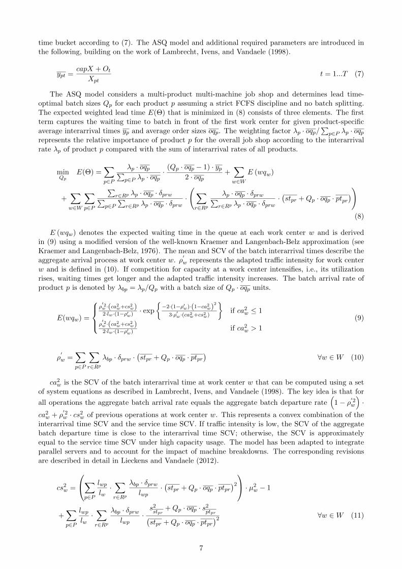
time bucket according to (7). The ASQ model and additional required parameters are introduced inthe following, building on the work of Lambrecht, Ivens, and Vandaele (1998).

ypt =capX +Ot

Xptt = 1...T (7)

The ASQ model considers a multi-product multi-machine job shop and determines lead time-optimal batch sizes Qp for each product p assuming a strict FCFS discipline and no batch splitting.The expected weighted lead time E(Θ) that is minimized in (8) consists of three elements. The firstterm captures the waiting time to batch in front of the first work center for given product-specificaverage interarrival times yp and average order sizes oqp. The weighting factor λp · oqp/

∑p∈P λp · oqp

represents the relative importance of product p for the overall job shop according to the interarrivalrate λp of product p compared with the sum of interarrival rates of all products.

minQp

E(Θ) =∑p∈P

λp · oqp∑p∈P λp · oqp

· (Qp · oqp − 1) · yp2 · oqp

+∑w∈W

E (wqw)

+∑w∈W

∑p∈P

∑r∈Rp λp · oqp · δprw∑

p∈P∑

r∈Rp λp · oqp · δprw·

(∑r∈Rp

λp · oqp · δprw∑r∈Rp λp · oqp · δprw

·(stpr +Qp · oqp · ptpr

))(8)

E (wqw) denotes the expected waiting time in the queue at each work center w and is derivedin (9) using a modified version of the well-known Kraemer and Langenbach-Belz approximation (seeKraemer and Langenbach-Belz, 1976). The mean and SCV of the batch interarrival times describe theaggregate arrival process at work center w. ρ

′w represents the adapted traffic intensity for work center

w and is defined in (10). If competition for capacity at a work center intensifies, i.e., its utilizationrises, waiting times get longer and the adapted traffic intensity increases. The batch arrival rate ofproduct p is denoted by λbp = λp/Qp with a batch size of Qp · oqp units.

E(wqw) =

ρ′2w ·(ca2w+cs2w)2·lw·(1−ρ′w) · exp

{−2·(1−ρ′w)·(1−ca2w)

2

3·ρ′w·(ca2w+cs2w)

}if ca2w ≤ 1

ρ′2w ·(ca2w+cs2w)2·lw·(1−ρ′w) if ca2w > 1

(9)

ρ′w =

∑p∈P

∑r∈Rp

λbp · δprw ·(stpr +Qp · oqp · ptpr

)∀w ∈W (10)

ca2w is the SCV of the batch interarrival time at work center w that can be computed using a setof system equations as described in Lambrecht, Ivens, and Vandaele (1998). The key idea is that for

all operations the aggregate batch arrival rate equals the aggregate batch departure rate(

1− ρ′2w)·

ca2w + ρ′2w · cs2w of previous operations at work center w. This represents a convex combination of the

interarrival time SCV and the service time SCV. If traffic intensity is low, the SCV of the aggregatebatch departure time is close to the interarrival time SCV; otherwise, the SCV is approximatelyequal to the service time SCV under high capacity usage. The model has been adapted to integrateparallel servers and to account for the impact of machine breakdowns. The corresponding revisionsare described in detail in Lieckens and Vandaele (2012).

cs2w =

∑p∈P

lwplw·∑r∈Rp

λbp · δprwlwp

·(stpr +Qp · oqp · ptpr

)2 · µ2w − 1

+∑p∈P

lwplw·∑r∈Rp

λbp · δprwlwp

·s2stpr

+Qp · oqp · s2ptpr(stpr +Qp · oqp · ptpr

)2 ∀w ∈W (11)

7

The SCV of the aggregate batch processing time (cs2w) is derived in (11). The term lwp =∑r∈Rp λbp · δprw denotes the aggregate batch arrival rate of product p at work center w, while

lw =∑

w∈W∑

r∈Rp λbp · δprw is the aggregate arrival rate at work center w of all products com-bined. Consequently, lwp/lw measures the probability that a product in front of work center w is oftype p. µw represents the aggregate processing rate at work center w and is derived in (12).

1

µw=

∑p∈P

lwplw·∑r∈Rp

λbp · δprwlwp

·(stpr +Qp · oqp · ptpr

) ∀w ∈W (12)

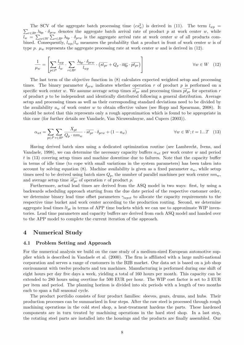
The last term of the objective function in (8) calculates expected weighted setup and processingtimes. The binary parameter δprw indicates whether operation r of product p is performed on aspecific work center w. We assume average setup times stpr and processing times ptpr for operation rof product p to be independent and identically distributed following a general distribution. Averagesetup and processing times as well as their corresponding standard deviations need to be divided bythe availability aw of work center w to obtain effective values (see Hopp and Spearman, 2008). Itshould be noted that this represents only a rough approximation which is found to be appropriate inthis case (for further details see Vandaele, Van Nieuwenhuyse, and Cupers (2003)).

αwt =∑p∈P

∑r∈Rp

Xpt

Qp · nmw· stpr · δprw + (1− aw) ∀w ∈W ; t = 1...T (13)

Having derived batch sizes using a dedicated optimization routine (see Lambrecht, Ivens, andVandaele, 1998), we can determine the necessary capacity buffers αwt per work center w and periodt in (13) covering setup times and machine downtime due to failures. Note that the capacity bufferin terms of idle time (to cope with small variations in the system parameters) has been taken intoaccount by solving equation (8). Machine availability is given as a fixed parameter aw, while setuptimes need to be derived using batch sizes Qp, the number of parallel machines per work center nmw,and average setup time stpr of operation r of product p.

Furthermore, actual lead times are derived from the ASQ model in two ways: first, by using abackwards scheduling approach starting from the due date period of the respective customer order,we determine binary lead time offset parameters γwpzt to allocate the capacity requirements to therespective time bucket and work center according to the production routing. Second, we determineaggregate lead times ltpt in terms of APP time buckets which we can use to approximate WIP inven-tories. Lead time parameters and capacity buffers are derived from each ASQ model and handed overto the APP model to complete the current iteration of the approach.

4 Numerical Study

4.1 Problem Setting and Approach

For the numerical analysis we build on the case study of a medium-sized European automotive sup-plier which is described in Vandaele et al. (2000). The firm is affiliated with a large multi-nationalcorporation and serves a range of customers in the B2B market. Our data set is based on a job shopenvironment with twelve products and ten machines. Manufacturing is performed during one shift ofeight hours per day five days a week, yielding a total of 160 hours per month. This capacity can beextended to 280 hours using overtime for 500 EUR per hour. The WIP cost factor is set to 3 EURper item and period. The planning horizon is divided into six periods with a length of two monthseach to span a full seasonal cycle.

The product portfolio consists of four product families: sleeves, gears, drums, and hubs. Theirproduction processes can be summarized in four steps. After the raw steel is processed through roughmachining operations in the cold steel shop, a heat-treatment hardens the parts. These hardenedcomponents are in turn treated by machining operations in the hard steel shop. In a last step,the rotating steel parts are installed into the housings and the products are finally assembled. Our

8

Figure 1: Product routings, machine data, and setup and processing times

case focuses on the first production phase which is the raw steel department. Figure 1 summarizesthe master data pertaining to the machines and product routings as well as the ranges of setup andprocessing times. The processing times are deterministic while the setup times exhibit a certain degreeof variability due to the complexity of the manual setup activities. The ranges of corresponding SCVsof the setup times are also given in Figure 1.

Demand follows a seasonal pattern with the base demand per product as shown in Table 1. Modeledas a harmonic oscillation, the demand peaks in the middle of the planning period and has a maximalamplitude according to a prespecified seasonality factor. Since the company in focus operates inan MTO setting, final goods inventories are non-existent. Every demand must be satisfied in therespective period and cannot be delayed beyond the due date. Besides the seasonal pattern, thearrivals of customer orders can exhibit variability which we investigate further below.

Following our approach described above, we generate several scenarios as a full factorial designof CM options and parameter constellations. The firm can source from two contractors that differin terms of flexibility and price. Flexibility in this context relates to the range of products and themaximum volumes that can be commissioned to the contractor. Price levels are reflected in the unitcost of CM. We consider three CM options: single sourcing from an inflexible or flexible contractor

Product name Base demand

Clutch Drum 1 95Clutch Drum 2 594

Drum 1 1,320Drum 2 679

Gear 54 Teeth 651Gear 65 Teeth 849Gear 69 Teeth 54

Hub 458Sleeve 1 189Sleeve 2 500Sleeve 3 349Sleeve 4 236

Table 1: Product master data

9

and a mixed setting with dual sourcing. The flexible contractor is capable of providing 35% of thebase demand of every product for a given unit price between 3 and 15 EUR. The inflexible contractoris more limited and can only deliver 20% of the base demand of the drums and hubs, albeit at a pricediscount of 35% compared with the flexible contractor.

Parameter constellations

Setup variabilitylow values given in the base case

moderate constant term of 0.3 and scaling factor of 1.2high constant term of 0.8 and scaling factor of 2.0

Demand variabilitydeterministic SCV of demand = 0.0

moderate SCV of demand = 1.0high SCV of demand = 2.5

Demand seasonalityflat seasonality factor = 10%

fluctuating seasonality factor = 35%

Table 2: Parameter constellations for the scenario analysis

We consider three sources of uncertainty for the parameter constellations: setup time variability,demand variability, and demand seasonality. For the setup time variability, we distinguish threestates (low, moderate, high) with respect to the product- and operation-specific SCVs. The case oflow variability is characterized by the base data given in Figure 1. We apply a linear transformation tothe values of the base case in order to consider moderate and high variability of setup times. Demandvariability originates from volatile customer order behavior and is captured in product-specific SCVsfor which we also investigate three distinct cases: deterministic demand as well as moderate and highdemand variability. Distinct demand seasonality factors complete the parameter constellations in focusand cover flat versus fluctuating demand over the planning period. The parameter constellations aresummarized in Table 2.

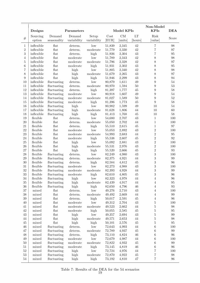
Creating a full factorial design of CM options and parameter constellations, we obtain 54 scenariosfor which we need to conduct the aggregate planning approach and an independent assessment of thequalitative factors. Aggregate planning is performed using IBM ILOG OPL with CPLEX v12.6.0.0for the APP model and a steepest descent algorithm implemented in C++ for the ASQ model. Theiterative solution procedure was run on an Intel Core i5 machine with 1.8 GHz per core and 4 GBRAM, resulting in computation times of around four minutes per scenario. The algorithm terminateson average after three to four iterations. While the execution of the APP and ASQ models requiresonly a few seconds, the data consolidation and transformation between the calculation steps accountsfor most of the computation time.

From the aggregate planning models we obtain CM volumes, aggregate order lead times, and totalrelevant costs. CM volumes represent the total number of production units that are sourced from acontractor over the course of the planning period. Aggregate order lead times are derived as weightedaverages across planning periods and products according to the internal production volumes. Totalrelevant costs are calculated as the sum of overtime, CM, and WIP costs over the planning period andcan be extracted from the objective function of the APP model.

In order to illustrate our approach, we apply a single metric to capture outsourcing risk as the majorqualitative factor in our case with an ordinal scale from 1 (low risk) to 10 (high risk). In practice,these values are assessed through structured interviews and consensus group decision-making withrelevant stakeholders. For the purpose of this paper and without loss of generality, we rely on theobservation that a scenario with an inflexible contractor as well as high demand seasonality and highdemand and/or setup variability exhibits the highest risk. In contrast, the lowest risk level is observedwhen a flexible contractor is opted for in a setting with low seasonality and low variability in demandand setup times. By applying a combinatorial scheme, we obtain risk assessments for each of the 54scenarios.

Our DEA approach combines two inputs (risk, costs) and two outputs (external CM quantities,internal aggregate order lead times) which are all measured in categorically distinct units of measure:

10

number, monetary units, and time. For our calculations, the lead time metric is inverted to ensure apositive correlation between inputs and outputs, since a shorter lead time represents a higher output.The DEA efficiency scores are derived using SAS/OR 13.1 at negligible run times. The results of theaggregate planning models, the independent assessment of qualitative factors, and the DEA efficiencyscores are summarized in Table 7 for the respective scenarios.

4.2 Discussion of the Results

In the following, we concentrate on interpreting the results pertaining to the selection of beneficial CMoptions and the implications of such a selection on operational performance. The overall results aresummarized in Table 3 along the three sourcing options, showing minimum, average, and maximumefficiency scores across the parameter constellations. A single sourcing agreement with the inflexiblecontractor yields a mean value of only 76 while single sourcing with the flexible contractor and dualsourcing result in considerably higher mean efficiency values of 97 and 98, respectively. Comparing theefficiency values, we observe a wide range of outcomes between 52 and 98 for the inflexible contractoroption in contrast to significantly narrower ranges for the flexible contractor option (92–100) and dualsourcing (95–100). We conclude that the flexible contractor option as well as dual sourcing largelyoutperform outsourcing to the inflexible contractor and lead to more robust results, since the efficiencyscores are higher on average and exhibit less variability.

Sourcing DEA Efficiency ScoresOption Minimum Average Maximum

flexible 92 97 100mixed 95 98 100

inflexible 52 76 98

Table 3: Minimum, average, and maximum DEA scores

Continuing the investigation of the DEA results, we create partial views in terms of envelope curvesalong the input and output dimensions. This allows us to highlight additional characteristics of thesolutions while keeping visualization complexity at a reasonable level. Since the partial views shownin Figures 2 and 3 cover only one output factor at a time, we need to consider the overall efficiencyscores of the scenarios to interpret the results. To achieve this we highlight efficient scenarios from theoverall DEA in black. Both partial views confirm that scenarios with the inflexible sourcing option areinferior to those involving the flexible contractor arrangement with the scenarios involving the mixedsetting falling in between.

Analyzing the results for the output dimension CM volume, one can see on the vertical axisthat higher risk penalizes the inflexible contractor option more than the mixed arrangement, whichin turn is inferior to all scenarios involving the flexible contractor option. We conclude that thehigher risk is not compensated for by higher CM volumes and corresponding contractor productivity.Reasoning horizontally, the ratio of CM volumes to costs clearly discriminates between the settingwith an inflexible contractor and the other two sourcing options. However, the cost dimension doesnot discriminate between the flexible and the mixed sourcing setting. As there are some efficientscenarios below the efficient curve of this partial view, we conclude that lead time obviously has anadditional efficiency impact on the scenario ranking.

Comparing scenario clusters in Figure 2, one can see the impact of demand fluctuation on theefficiency of distinct sourcing options. While we observe a clear separation for the inflexible contractoroption (scenarios 1–9 vs. 10–18) and the mixed sourcing arrangement (scenarios 37–45 vs. 46–54),there is no analogous separation for the scenarios involving the flexible contractor option. This can beexplained by the small product range and limited production volumes that can be commissioned tothe inflexible contractor. As a consequence, the company cannot leverage the inflexible contractor tofully accommodate seasonal demand fluctuation, which results in lower contractor productivity andlower efficiency scores. Even in a mixed-source setting with additional benefits from lower CM costs,the negative impact of inflexibility on overall efficiency remains.

11

Figure 2: Envelope curve relating CM volumes to risk and costs

Examining the partial view of the lead time dimension (see Figure 3), we also observe the negativeimpact of demand fluctuation on the efficiency scores for the respective scenarios (scenarios 10–18,28–36, and 46–54). While the flexible contractor can fully compensate for the negative impact viaimproved contractor productivity (see the black-colored items) at least for selective scenarios, allsourcing options exhibit comparably low efficiency scores for the lead time dimension in relation toboth risk and costs. Comparing scenarios 1–9 vs. 37–45, one can see that, for flat demand patterns,both sourcing from the inflexible contractor and mixed sourcing result in comparably high efficiencyvalues. Despite this, mixed sourcing exhibits a slightly lower risk exposure.

In the following, we examine the operational performance metrics of the stochastic manufacturingsystem in greater detail to investigate the impact of demand and setup variability as well as demandseasonality. Starting with demand seasonality, we compare average aggregate batch sizes and averageaggregate lead times for flat and fluctuating demand. From Table 4 one can see opposing effects: whileaverage aggregate batch sizes (+1.9%) and lead times (+3.1%) increase with outsourcing flexibilityunder flat demand, corresponding batch sizes (-5.8%) and lead times (-6.2%) decrease when demandfluctuates over time. This can be explained by the fact that outsourcing serves distinct purposes in thetwo cases. With flat demand, outsourcing is used to improve utilization by commissioning volumes ofselective products to the contractor, which reduces non-productive setup times and allows for largerbatch sizes. In contrast, when demand fluctuates, external production serves as a secondary capacityon a larger scale to smoothen operating levels with the respective effects on batch sizes and lead times.

Assuming moderate demand and setup variability, we further analyze the case of flat vs. fluctuatingdemand in Figure 4 using illustrative scenario results. In general, we observe significantly higher

Flat demand Fluctuating demand

Averge Average Average AverageSourcing aggregate aggregate aggregate aggregateOption batch size lead time batch size lead time

flexible 110.1 43.9 102.1 44.4mixed 109.5 43.9 103.3 45.2

inflexible 108.0 42.6 108.4 47.3

Table 4: Average aggregate batch sizes and lead times given flat vs. fluctuating demand

12

Figure 3: Envelope curve relating aggregate order lead times (LT) to risk and costs

relevant costs (+47–56%) associated with managing operations when demand fluctuates. The changesin average batch sizes support the abovementioned general findings. In both settings, overtime is usedonly with the inflexible contractor option. Higher flexibility of the contractor implies rising CM costsand a shift towards external production. Under a fully flexible outsourcing agreement and flat demand,40% of the costs are allocated to CM. This figure rises as high as 60% if demand seasonality increasesfrom flat to fluctuating. While the combination of an inflexible and a flexible contractor deliversmediocre results in terms of batch sizes and lead times, this setting yields the lowest-cost solution inboth cases, with savings of about 10% compared with the results of a single sourcing agreement withthe flexible contractor.

Sourcing Demand variability Setup variability

Option Low Moderate High Low Moderate High

flexible 110.4 110.1 109.7 109.4 109.9 110.9mixed 109.4 109.5 109.6 108.9 109.4 110.3

inflexible 107.8 107.9 108.2 107.4 108.0 108.6

Table 5: Average aggregate batch sizes for various demand and setup variability parameters given flatdemand

Building on the previous results, we examine the impact of demand and setup variability separatelyfor flat and fluctuating demand. From Table 5 one can see that the findings on outsourcing flexibilityunder flat demand still hold, i.e., average batch sizes increase with outsourcing flexibility, which isalso confirmed by the respective external and internal production volumes. Comparing the results fordiffering levels of variability, we conclude that demand variability has virtually no impact on averageaggregate batch sizes (±0.4%) while rising setup variability appears to increase average aggregatebatch sizes (+1.1–1.3%), which is also true for the corresponding aggregate lead times. The effect ofincreasing batch sizes can be explained by the fact that the company offsets the negative impact ofrising setup variability by building fewer but larger batches.

As can be seen from Table 6, the abovementioned findings on outsourcing flexibility for the case offluctuating demand are reinforced for settings with the flexible contractor option or a mixed sourcingarrangement, i.e., average aggregate batch size decreases as outsourcing flexibility increases. Exam-ining the impact of demand and setup variability, we observe similar results as for the case of flat

13

Figure 4: Cost breakdown for selected scenarios given flat vs. fluctuating demand

Sourcing Demand variability Setup variability

Option Low Moderate High Low Moderate High

flexible 102.1 102.0 102.2 100.9 101.8 103.6mixed 103.2 103.3 103.5 102.1 103.0 104.8

inflexible 109.7 109.9 105.5 112.7 110.1 102.3

Table 6: Average aggregate batch sizes for various demand and setup variability parameters givenfluctuating demand

demand: virtually no changes in batch sizes for differing levels of demand variability (±0.2%) andincreasing batch sizes for higher setup variability (+2.7%), which are even amplified due to demandfluctuation. However, we obtain converse results for the case of single sourcing from the inflexible con-tractor: (i) considerably lower batch sizes when demand/setup variability is high and (ii) decreasingbatch sizes when setup variability rises.

To further investigate the aforementioned matter, we conduct a breakdown for selected scenariosas shown in Figures 5 and 6, comparing inflexible and flexible sourcing options for various parametersof demand and setup variability. Analyzing the cost split as well as related internal and externalproduction volumes, we conclude that in a setting with a flexible contractor additional variability canbe passed on to the contractor with only marginal increases in total relevant costs. In contrast, withthe inflexible sourcing option, the company needs to manage part of the variability on its own. Sinceboth types of variability drive batch lead times and WIP, the company reduces average batch sizesto reduce WIP costs. However, this comes at the cost of additional CM volumes and overtime tocompensate for the additional capacity loss due to setups.

5 Conclusion and Outlook

In this paper, we proposed a novel approach to address the strategic-tactical issue of outsourcingdecision-making in a stochastic manufacturing environment. Our contribution is twofold: first, wepresented a robust multi-criteria approach that considers multiple quantitative as well as qualitativefactors and that accounts for parameter uncertainty. For this purpose, a DEA-based approach was

14

Figure 5: Cost breakdown for selected scenarios:focus demand variability

Figure 6: Cost breakdown for selected scenarios:focus setup variability

applied to rank several outsourcing options under various parameter constellations. Second, we in-troduced an APP approach for stochastic manufacturing environments with CM options to obtainoperational performance metrics for the DEA. To this end, an aggregate stochastic queuing modelwas combined with a conventional APP model to capture workload-dependent lead times as well ascapacity losses due to setup times and machine breakdowns.

A real-life case example was used to highlight our approach in which costs and risk exposureof the manufacturing system in focus were balanced against contractor productivity and customerservice, which we represented by aggregate order lead times. For the analysis, we used a combinationof overall efficiency scores and partial views of envelope curves to ease representation of the resultsgiven the multi-dimensional approach of DEA. These methods appeared to be very instructive andcould support S&OP meetings with management professionals that have only limited knowledge ofOR methods. Although we have only considered an illustrative example, the study revealed somegeneral insights with respect to capacity management and outsourcing in stochastic manufacturingenvironments. Demand fluctuation appears to be the single most important factor that influencesoperational performance and determines the strategic role of outsourcing in this setting. Demand andoperations variability have only minor effects on operational metrics given the fact that outsourcingoptions can compensate for them.

For future research, one can generalize the approach to include other types of decisions that areat stake in the S&OP context. This could include, for instance, aspects of new product introductionand profitable-to-promise planning. In this work, we integrated outsourcing risk as the single mostrelevant qualitative factor. However, there are many additional intangible criteria such as sustain-ability, strategic fit, or managerial complexity that could be considered to this end. Furthermore,this approach could be applied to a process industry context to elaborate on the impact of variableprocessing times and more complex changeover processes as well as product routings. Some additionalwork could be done from a methodological perspective by improving the aggregate stochastic queuingmodel with respect to batch splitting or the modeling of machine repair activities. Moreover, therobust DEA approach should be investigated further to examine novel methods for scenario analysisas well as for visualizing and interpreting the results.

Acknowledgment

The authors gratefully acknowledge financial support from the GlaxoSmithKline Research Chair onOperations Management and the CAMELOT Management Consultants Endowed Assistant Profes-sorship for Supply Chain Management.

15

References

Almeder, Christian, Margaretha Preusser, and Richard F. Hartl. 2009. “Simulation and optimizationof supply chains: Alternative or complementary approaches?.” OR Spectrum 31 (1): 95–119.

Armbruster, Dieter, and Reha Uzsoy. 2012. “Continuous dynamic models, clearing functions, anddiscrete-event simulation in aggregate production planning.” In TutORials in Operations Research:New directions in informatics, optimization, logistics, and production, edited by Pitu B. Mirchan-dani. 103–126. Hanover: INFORMS.

Arrunada, Benito, and Xose H. Vazquez. 2006. “When your contract manufacturer becomes yourcompetitor.” Harvard Business Review 84 (9): 135–144.

Asmundsson, Jakob, Ronald L. Rardin, Can Hulusi Turkseven, and Reha Uzsoy. 2009. “Productionplanning with resources subject to congestion.” Naval Research Logistics 56 (2): 142–157.

Atamturk, Alper, and Dorit S. Hochbaum. 2001. “Capacity acquisition, subcontracting, and lot sizing.”Management Science 47 (8): 1081–1100.

Bang, June-Young, and Yeong-Dae Kim. 2010. “Hierarchical production planning for semiconductorwafer fabrication based on linear programming and discrete-event simulation.” IEEE Transactionson Automation Science and Engineering 7 (2): 326–336.

Carravilla, Maria Antonia, and Jorge Pinho de Sousa. 1995. “Hierarchical production planning in amake-to-order company: A case study.” European Journal of Operational Research 86 (1): 43–56.

Charnes, Abraham, William W. Cooper, and Edwardo Rhodes. 1978. “Measuring the efficiency ofdecision making units.” European Journal of Operational Research 2 (6): 429–444.

de Boer, Luitzen, Eva Labro, and Pierangela Morlacchi. 2001. “A review of methods supportingsupplier selection.” European Journal of Purchasing & Supply Management 7 (2): 75–89.

Dotoli, Mariagrazia, and Maddalena Falagario. 2012. “A hierarchical model for optimal supplier se-lection in multiple sourcing contexts.” International Journal of Production Research 50 (11): 2953–2967.

Gansterer, Margaretha, Christian Almeder, and Richard F. Hartl. 2014. “Simulation-based optimiza-tion methods for setting production planning parameters.” International Journal of ProductionEconomics 151: 206–213.

Gottfredson, Mark, Rudy Puryear, and Stephen Phillips. 2005. “Strategic sourcing: From peripheryto the core.” Harvard Business Review 83 (2): 132–139.

Graves, Stephen C. 1986. “A tactical planning model for a job shop.” Operations Research 34 (4):522–533.

Hahn, Gerd J., Chris Kaiser, Heinrich Kuhn, Lien Perdu, and Nico J. Vandaele. 2012. “Enhancingaggregate production planning with an integrated stochastic queuing model.” In Operations ResearchProceedings 2011, edited by Diethard Klatte, Hans-Jakob Luthi, and Karl Schmedders. 451–456.Berlin: Springer.

Hahn, Gerd J., and Heinrich Kuhn. 2012. “Value-based performance and risk management in supplychains: A robust optimization approach.” International Journal of Production Economics 139 (1):135–144.

Helper, Susan. 1991. “Strategy and irreversibility in supplier relations: The case of the U.S. automobileindustry.” The Business History Review 65 (4): 781–824.

16

Ho, William, Xiaowei Xu, and Prasanta K. Dey. 2010. “Multi-criteria decision making approaches forsupplier evaluation and selection: A literature review.” European Journal of Operational Research202 (1): 16–24.

Hopp, Wallace J., and Mark L. Spearman. 2008. Factory physics. 3rd ed. New York: McGraw-Hill/Irwin.

Hung, Yi-Feng, and Robert C. Leachman. 1996. “A production planning methodology for semicon-ductor manufacturing based on iterative simulation and linear programming calculations.” IEEETransactions on Semiconductor Manufacturing 9 (2): 257–269.

Jansen, Michiel M., Ton G. de Kok, and Jan C. Fransoo. 2013. “Lead time anticipation in supplychain operations planning.” OR Spectrum 35 (1): 251–290.

Kacar, Necip B., Durmus F. Irdem, and Reha Uzsoy. 2012. “An experimental comparison of productionplanning using clearing functions and iterative linear programming-simulation algorithms.” IEEETransactions on Semiconductor Manufacturing 25 (1): 104–117.

Karmarkar, Uday S. 1987. “Lot sizes, lead times and in-process inventories.” Management Science 33(3): 409–418.

Kim, Bowon. 2003. “Dynamic outsourcing to contract manufacturers with different capabilities ofreducing the supply cost.” International Journal of Production Economics 86 (1): 63–80.

Kraemer, Wolfgang, and Manfred Langenbach-Belz. 1976. Approximate formulae for the delay in thequeueing system GI/G/1. Congressbook Eighth International Teletraffic Congress.

Kuo, Ren Jie, and Y. J. Lin. 2012. “Supplier selection using analytic network process and dataenvelopment analysis.” International Journal of Production Research 50 (11): 2852–2863.

Lambrecht, Marc R., Philip L. Ivens, and Nico J. Vandaele. 1998. “ACLIPS: A capacity and lead timeintegrated procedure for scheduling.” Management Science 44 (11): 1548–1561.

Lieckens, Kris, and Nico J. Vandaele. 2012. “Multi-level reverse logistics network design under uncer-tainty.” International Journal of Production Research 50 (1): 23–40.

Manufacturing Market Insider. 2014. “MMI articles.” Retrieved July 25, 2014, fromhttp://mfgmkt.com/mmi-articles.html.

Merzifonluoglu, Yasemin, Joseph Geunes, and H. Edwin Romeijn. 2007. “Integrated capacity, demand,and production planning with subcontracting and overtime options.” Naval Research Logistics 54(4): 433–447.

Missbauer, Hubert. 2011. “Order release planning with clearing functions: A queueing-theoreticalanalysis of the clearing function concept.” International Journal of Production Economics 131 (1):399–406.

Missbauer, Hubert, and Reha Uzsoy. 2011. “Optimization models of production planning problems.”In Planning Production and Inventories in the Extended Enterprise, edited by Karl G. Kempf, PınarKeskinocak, and Reha Uzsoy. 437–507. Boston: Springer.

Mula, Josefa, Raul Poler, Jose Pedro Garcıa-Sabater, and Francisco Cruz Lario. 2006. “Models forproduction planning under uncertainty: A review.” International Journal of Production Economics103 (1): 271–285.

Nam, Sang-Jin, and Rasaratnam Logendran. 1992. “Aggregate production planning: A survey ofmodels and methodologies.” European Journal of Operational Research 61 (3): 255–272.

Pahl, Julia, Stefan Voß, and David L. Woodruff. 2007. “Production planning with load dependent leadtimes: An update of research.” Annals of Operations Research 153 (1): 297–345.

17

Plambeck, Erica L., and Terry A. Taylor. 2005. “Sell the plant? The impact of contract manufacturingon innovation, capacity, and profitability.” Management Science 51 (1): 133–150.

Schneeweiss, Christoph. 2003. “Distributed decision making: A unified approach.” European Journalof Operational Research 150 (2): 237–252.

Selcuk, Baris, Jan C. Fransoo, and A. G. de Kok. 2008. “Work-in-process clearing in supply chainoperations planning.” IIE Transactions 40 (3): 206–220.

van Arnum, Patricia. 2000. “Bulls or bears? Outlook in contract manufacturing.” Chemical MarketReporter 257 (7): FR3–FR6.

Vandaele, Nico J., and Catherine J. Decouttere. 2013. “Sustainable R&D portfolio assessment.” De-cision Support Systems 54 (4): 1521–1532.

Vandaele, Nico J., Marc R. Lambrecht, Nicolas de Schuyter, and Rony Cremmery. 2000. “Spicer Off-Highway Products Division-Brugge improves its lead-time and scheduling performance.” Interfaces30 (1): 83–95.

Vandaele, Nico J., Inneke Van Nieuwenhuyse, and Sascha Cupers. 2003. “Optimal grouping for anuclear magnetic resonance scanner by means of an open queueing model.” European Journal ofOperational Research 151 (1): 181–192.

18

Non-ModelDesigns Parameters Model KPIs KPIs DEA

#Sourcing Demand Demand Setup Cost CM LT Risk

Scoreoption seasonality variability variability [EUR] [units] [hours] [value]

1 inflexible flat determ. low 51,839 2,345 42 7 982 inflexible flat determ. moderate 51,779 2,330 42 7 973 inflexible flat determ. high 51,926 2,304 43 7 954 inflexible flat moderate low 51,789 2,343 42 8 985 inflexible flat moderate moderate 51,796 2,328 42 8 976 inflexible flat moderate high 51,931 2,302 43 8 957 inflexible flat high low 51,805 2,340 42 8 988 inflexible flat high moderate 51,679 2,265 43 8 979 inflexible flat high high 51,946 2,299 43 8 9410 inflexible fluctuating determ. low 80,879 1,611 49 9 5411 inflexible fluctuating determ. moderate 80,970 1,594 50 9 5312 inflexible fluctuating determ. high 81,397 1,777 45 9 5813 inflexible fluctuating moderate low 80,918 1,607 49 9 5414 inflexible fluctuating moderate moderate 81,027 1,589 50 9 5215 inflexible fluctuating moderate high 81,396 1,773 45 9 5816 inflexible fluctuating high low 80,982 1,599 49 10 5417 inflexible fluctuating high moderate 81,628 1,806 44 10 6018 inflexible fluctuating high high 81,413 1,768 45 10 5819 flexible flat determ. low 54,680 2,707 43 1 10020 flexible flat determ. moderate 55,050 2,702 44 1 10021 flexible flat determ. high 55,510 2,615 45 1 9722 flexible flat moderate low 55,053 2,892 43 2 10023 flexible flat moderate moderate 54,993 2,683 44 2 9524 flexible flat moderate high 55,538 2,607 45 2 9225 flexible flat high low 55,092 2,881 43 2 10026 flexible flat high moderate 55,531 2,976 43 2 10027 flexible flat high high 55,520 2,666 45 2 9328 flexible fluctuating determ. low 82,249 4,980 43 3 10029 flexible fluctuating determ. moderate 82,375 4,921 44 3 9930 flexible fluctuating determ. high 82,584 4,812 45 3 9631 flexible fluctuating moderate low 82,273 4,988 43 3 10032 flexible fluctuating moderate moderate 82,393 4,928 44 3 9933 flexible fluctuating moderate high 82,610 4,805 45 3 9634 flexible fluctuating high low 82,323 4,978 44 4 9635 flexible fluctuating high moderate 82,439 4,917 44 4 9536 flexible fluctuating high high 82,650 4,796 46 4 9337 mixed flat determ. low 49,276 2,710 43 4 10038 mixed flat determ. moderate 49,492 2,669 44 4 9939 mixed flat determ. high 50,017 2,591 45 4 9640 mixed flat moderate low 49,312 2,704 43 5 10041 mixed flat moderate moderate 49,523 2,662 44 5 9842 mixed flat moderate high 50,055 2,585 45 5 9543 mixed flat high low 49,357 2,694 43 5 9944 mixed flat high moderate 49,571 2,653 44 5 9845 mixed flat high high 50,101 2,576 45 5 9546 mixed fluctuating determ. low 72,643 4,993 44 6 10047 mixed fluctuating determ. moderate 72,789 4,937 45 6 9948 mixed fluctuating determ. high 73,110 4,824 46 6 9649 mixed fluctuating moderate low 72,679 4,987 44 6 10050 mixed fluctuating moderate moderate 72,822 4,932 45 6 9951 mixed fluctuating moderate high 73,145 4,819 46 6 9652 mixed fluctuating high low 72,724 4,976 44 7 10053 mixed fluctuating high moderate 72,870 4,922 45 7 9854 mixed fluctuating high high 73,192 4,810 47 7 96

Table 7: Results of the DEA for the 54 scenarios19

FACULTY OF ECONOMICS AND BUSINESS Naamsestraat 69 bus 3500

3000 LEUVEN, BELGIË tel. + 32 16 32 66 12 fax + 32 16 32 67 91

info@econ.kuleuven.be www.econ.kuleuven.be