a monte carlo approach to joint probability of wave, tide … · · 2017-07-15executive health...

Executive Health and Safety

A Monte Carlo approach to joint probability of wave, tide and surge in extreme water level calculations

Prepared by PhysE Limited for the Health and Safety Executive 2009

RR740 Research Report


A Monte Carlo approach to joint probability of wave, tide and surge in extreme water level calculations

Joseph P Fox MPhys PhD PhysE Limited The Harbour Offices The Quay Yarmouth Isle of Wight PO41 0NT

Extreme Water Level is the total level of the water arising from wave crest, storm surge and tidal level acting in combination with each other throughout an extreme event. Individually, each of these components is relatively well understood. However, the combination of these components is not straightforward and depends on the conditions of the location in question. This study addresses the behaviour of the individual components, their interaction, and their joint probability, leading to the development of a Monte Carlo based approach to the estimation of Extreme Water Level. The study concludes with a review of latest ISO guidance on estimating extreme water levels and a comparison between extreme water level results derived using existing methods, ISO guidance and Monte Carlo simulations.

This report and the work it describes were funded by the Health and Safety Executive (HSE). Its contents, including any opinions and/or conclusions expressed, are those of the author alone and do not necessarily reflect HSE policy.

HSE Books

© Crown copyright 2009

First published 2009

All rights reserved. No part of this publication may be reproduced, stored in a retrieval system, or transmitted in any form or by any means (electronic, mechanical, photocopying, recording or otherwise) without the prior written permission of the copyright owner.

Applications for reproduction should be made in writing to:Licensing Division, Her Majesty’s Stationery Office,St Clements House, 2-16 Colegate, Norwich NR3 1BQor by e-mail to [email protected]

ii

TABLE OF CONTENTS

EXECUTIVE SUMMARY ................................................................................... 7

1. BACKGROUND ........................................................................................ 1

2. DATA ........................................................................................................ 4

2.1 MEASURED DATA.................................................................................................... 42.2 MODEL DATA.......................................................................................................... 42.3 OVERVIEW OF MAXIMA AND ASSOCIATED VALUES .................................................... 5

3. WAVE CREST........................................................................................... 6

3.1 KROGSTAD/BORGMAN INTEGRAL ............................................................................. 73.2 TROMANS & VANDERSCHUREN METHOD .................................................................. 9

4. TIDES...................................................................................................... 12

4.1 INFLUENCE OF TIDE ON SURGE AND WAVES........................................................... 13

5. STORMS ................................................................................................. 21

6. RELATIONSHIP BETWEEN SURGE AND WAVE HEIGHT ................... 29

7. MONTE CARLO SIMULATIONS............................................................. 31

7.1 THE PROCESS....................................................................................................... 317.1.1 Wave heights ............................................................................................................ 317.1.2 Tidal heights............................................................................................................. 337.1.3 Surge heights............................................................................................................ 33

7.2 MONTE CARLO OUTPUT STATISTICS ...................................................................... 35

8. RESULTS................................................................................................ 36

8.1 100 YEAR RETURN PERIOD EXTREME WATER LEVELS ........................................... 368.2 10,000 YEAR RETURN PERIOD EXTREME WATER LEVELS ...................................... 378.3 COMMENTS ON 100 AND 1,000 YEAR EXTREME WATER LEVELS ............................. 388.4 MEASURED EXTREME WATER LEVELS.................................................................... 398.5 CALIBRATING THE SIMULATION .............................................................................. 408.6 100 AND 10,000 YEAR RETURN PERIOD EXTREME WATER LEVELS......................... 41

9. CONCLUSIONS ...................................................................................... 43

10. APPENDIX: SOFTWARE TESTING..................................................... 44

10.1 SOFTWARE TESTING.......................................................................................... 4410.1.1 Input Data............................................................................................................. 4410.1.2 Hs ......................................................................................................................... 4510.1.3 Surges ................................................................................................................... 4510.1.4 Tides ..................................................................................................................... 4810.1.5 Still water level ..................................................................................................... 4810.1.6 Summary............................................................................................................... 51

iii

FIGURES

Figure 1 Location of measured data sources used in this study........................................................................ 4Figure 2 Exceedence Distribution of Extreme Crest Elevation .......................................................................... 8Figure 3 Illustration of mean excess plot............................................................................................................. 10Figure 4 Probability of occurrence of measured tidal level (m) at Auk, K13 and Euro. Relative to MSL ... 12Figure 5 K13 measured: Probability of occurrence of maximum surge and maximum wave height relative

to high water.......................................................................................................................................... 14Figure 6 K13 Model: Probability of occurrence of maximum surge and maximum wave height relative to

high water. ............................................................................................................................................. 14Figure 7 Euro Measured: Probability of occurrence of maximum surge and maximum wave height

relative to high water............................................................................................................................ 15Figure 8 Euro model: Probability of occurrence of maximum surge and maximum wave height relative to

high water. ............................................................................................................................................. 15Figure 9 Auk Measured: Probability of occurrence of maximum surge and maximum wave height relative

to high water. Based on measured Auk data .................................................................................. 16Figure 10 Auk Model: Probability of occurrence of maximum surge and maximum wave height relative to

high water. ............................................................................................................................................. 16Figure 11 Auk Measured: Maximum Hs and SWL throughout the positive tide. ............................................. 18Figure 12 Auk Model: Maximum Hs and SWL throughout the positive tide. .................................................... 18Figure 13 K13 Measured: Maximum Hs and SWL throughout the positive tide. ............................................. 19Figure 14 K13 Model: Maximum Hs and SWL throughout the positive tide..................................................... 19Figure 15 Euro Measured: Maximum Hs and SWL throughout the positive tide............................................. 20Figure 16 Euro Model: Maximum Hs and SWL throughout the positive tide.................................................... 20Figure 17 Auk Measured: Surge duration analysis .............................................................................................. 22Figure 18 Auk Model: Surge duration analysis..................................................................................................... 22Figure 19 K13 Measured: Surge duration analysis.............................................................................................. 23Figure 20 K13 Model: Surge duration analysis based on model K13 data ...................................................... 23Figure 21 Euro Measured: Surge duration analysis ............................................................................................ 24Figure 22 Euro Model: Surge duration analysis ................................................................................................... 24Figure 23 Auk Measured: Time series plots of largest 5 surges........................................................................ 25Figure 24 K13 Measured: Time series plots of largest 5 surges........................................................................ 26Figure 25 Euro Measured: Time series plots of largest 5 surges ..................................................................... 27Figure 26 Auk Measured: Hs-Surge (positive only) scatter plot......................................................................... 30Figure 27 K13 Measured: Hs-Surge (positive only) scatter plot ........................................................................ 30Figure 28 Euro Measured: Hs-Surge (positive only) scatter plot ....................................................................... 30Figure 29 Monte Carlo: Input Specifications for Significant Wave Height ........................................................ 32Figure 30 Monte Carlo: Input Specifications for Tidal level ................................................................................ 33Figure 31 Monte Carlo: Input Specifications for Surge........................................................................................ 34Figure 32 Monte Carlo: Identification of the Surge ‘Scaling factor’.................................................................... 35Figure 33 Variation of 20 year EWL with decreasing scaling factor. The red dashed line represents the

measured 20 year extreme water level at K13................................................................................. 40Figure 34 Comparison between simulated and theoretical 100 year Hs values.............................................. 45Figure 35 Distribution of surges associated with the maximum crest+surge. .................................................. 46Figure 36 Distribution of surges associated with the maximum crest+surge. .................................................. 46Figure 37 Distribution of surges associated with the maximum crest+surge ................................................... 47Figure 38 Distribution of surges associated with the maximum crest+surge. .................................................. 47Figure 39 Distribution of tides associated with the maximum crest+tide. ......................................................... 48Figure 40 Distribution of SWL associated with the maximum crest+tide+surge.............................................. 49Figure 41 Distribution of SWL associated with the maximum crest+tide+surge.............................................. 49Figure 42 Distribution of SWL associated with the maximum crest+tide+surge.............................................. 50Figure 43 Distribution of SWL associated with the maximum crest+tide+surge.............................................. 50

iv

TABLES

Table 1 Key statistics from the measured and model data sets .....................................................................5Table 2 Comparison of Extreme Crest Elevation – Borgman & Monte Carlo ...............................................8Table 3 Height and Duration of the 5 largest Surges at Auk, K13 and Euro...............................................28Table 4 Comparison of 100 year Extreme Water Levels constituents calculated using various

techniques ..............................................................................................................................................36Table 5 Summary of 100 year Extreme Water Levels found using different techniques...........................37Table 6 Comparison of 100 year Extreme Water Levels constituents calculated using various

techniques ..............................................................................................................................................37Table 7 Summary of 10,000 year Extreme Water Levels found using different techniques .....................38Table 8 Summary of extrapolated total water levels at K13 ..........................................................................39Table 9 Summary of Monte Carlo Simulation inputs at K13..........................................................................40Table 10 Comparison of 100 and 10,000 year return periods at K13 ............................................................41

v

EXECUTIVE SUMMARY

Measured data from sites across the North Sea are used to investigate the individual and combined behaviour of the wave crest, storm surge and tidal level. The joint probability of the parameters is discussed and Monte Carlo simulations are proposed as a method of rigorously accounting for the joint probability of the individual components.

Software was developed and the results of Monte Carlo simulation compared with existing methods of estimating the extreme water level at the 100 and 10,000 year return periods.

Measured total water level data was used and comparisons made between the predicted 100 and 10,000 year extreme water level from the measured data and those predicted via Monte Carlo simulation and other methods, including those described in ISO-19902:2007.

Comparisons revealed that the Monte Carlo simulations provided a reliable method with which the extreme water level could be estimated. Furthermore, ISO-19902 describes ‘best’ and ‘worst’ cases which provide an envelope into which the predicted extreme water levels from all the other techniques used in this report fall. The techniques used in this report represent both historical and the most commonly used contemporary techniques for estimating extreme water levels. However, the list may not be exhaustive and other techniques may exist.

vii

1. BACKGROUND

Extreme Water Level (EWL) is a key parameter in the design and safe operation of offshore installations, particularly with respect to bottom founded structures. A wave impact on the topsides produces a significantly greater overturning moment than a wave passing through the platform legs1. EWL therefore determines the elevation of the base of the topsides.

EWL is defined as a combination of three components; • Wave crest • Tidal elevation • Surge (the variation in sea level induced my meteorological influences).

It is important to differentiate between EWL and Still Water Level (SWL). EWL includes the wave crest and is therefore a transient condition associated with water particle motions induced by waves. SWL does not include waves and defines the level due only to tide and surge acting together.

Between 1974 and 1996 offshore structures may have been designed according to the UK Guidance Notes2. Guidance for the derivation of extreme water levels given therein was that EWL may be derived through the direct superposition of crest heights calculated empirically from a sea state and surge amplitude (both with a 50 year return period) and the level Spring Tidal Amplitude (defined as M2 + S2). Hence:

EWL50 = (M2 + S2) + S+50 + Hcrest50

Where: EWL50 = Extreme Water Level with a 50-year return period M2 = Amplitude of the Lunar semi-diurnal tidal constituent S2 = Amplitude of the Solar semi-diurnal tidal constituent S+

50 = Amplitude of the surge with a 50-year return period Hcrest50 = Amplitude of the wave crest for the maximum wave height with a 50

year return period

For design, an air gap of 1.5 m between EWL and the base of the lowermost deck was recommended.

This approach might be described as unsophisticated because:

• The calculation of height of the wave crest does not take account of the possibility that the maximum wave might occur in a sea state which, although high, might not necessarily be the highest sea state.

• The derived value of Hcrest50 is the most probable value in the distribution of maxima. As such, there is a significant probability (nominally 63%, subject to the particular form of crest distribution applied) that the derived Hcrest50 will be exceeded.

• The tidal range may not be a mean spring tide.

1 Airgap Workshop HSE/E&P Forum Imperial College, London. 14-15 June 1999

2 The Offshore Installations (Construction and Survey) Regulations 1974 HMSO,1974. SI 1974 / 289 [Replaced by SI 1996 / 913 – The Offshore Installations and Wells (Design and Construction etc.) Regulations, 1996 – ISBN: 0 110 54451 X].

1

• The maximum crest may not occur at the time of high water. • The surge may not be a 50 year event, simply because the waves are a 50 year event. • The peak of surge may not be coincident with the highest wave. • The value of the 1.5 m air gap varied with the general exposure of the location – 1.5 m

provided a significantly smaller margin of safety in the northern North Sea than in the southern North Sea.

It should be noted that by the early 1980’s the larger oil and gas exploration and production companies were designing facilities to a return period of 100 years and applying variations on the 1974 recipe to account for joint probability of tide and surge, for example:

EWL100 = (M2 + S2) + S+50 + Hcrest100

In this case the implicit assumption was:

SWL100 = (M2 + S2) + S+50

…and some evidence to support this assumption was available from the analysis of long term sea level data sets at standard ports.

As a result of significantly greater temporal and spatial resolution in acquired oceanographic data, together with advances in computing and recent developments in formulating short-term statistics, potential shortcomings in the 1974 approach may be addressed. International Standard ISO 19901-1 published in 20053 addresses improvements to the estimation of the wave crest in some detail, but does not provide guidance with respect to the computation of the corresponding tide and surge components.

Latest guidance with respect to the incorporation of tide and surge may be found in ISO 19902:20074 which states

-----Beginning of quote-----

“…the deck elevation, h, above the mean sea level can be estimated [as follows]:

If a storm surge is not expected to occur at the same time as the abnormal wave crest:

h = √(a 2 + s 2 + t 2) + f

3 Petroleum and natural gas industries – Specific requirements for offshore structures Part 1: Metocean design and operating considerations BS EN ISO 19901-1:2005

4 Petroleum and natural gas industries – Fixed steel offshore structures ISO 19902:2007

2

If a storm surge is expected to occur at the same time as the abnormal wave crest:

h = √((a + s) 2 + t 2) + f

where: a is the abnormal wave crest height s is the extreme storm surge t is the maximum elevation of the tide relative to mean sea level f is the expected sum of subsidence, settlement and sea level rise over the design

service life of the structure.

For deep and intermediate water depths ‘a’ can be approximated to

a > 1.3 a100

a > a100 + 1.5m

awhere :

100 is the extreme wave crest height with a return period of 100 years.

The estimate for h obtained with this procedure is indicative and suitable for conceptual design studies. The owner should review the deck elevation prior to detailed design.

In general, no platform processing elements, piping, or equipment should be located below the lower deck in the designated air gap. However, when it is unavoidable to position such items as minor sub-cellars, sumps, drains, or production piping in the air gap, provisions should be made for the actions due to waves developed on these items.

NOTE: 1.5m is a traditional value used for air gap, but analysis of metocean data has shown that it does not always allow sufficient reliability in certain geographical areas.”

-----End of quote-----

The aim of this work in this report is therefore to:

a) Investigate the joint probability relationships between the key components of extreme water level; namely the tide, surge and wave data, and against that background to…

b) Establish a mathematically rigorous method for the estimation of EWL that can be implemented within the constraints of the data actually available within the public domain.

The work concludes that a Monte Carlo technique is appropriate to the task, this being particularly advantageous in that it can be run using data supplied as frequency distributions. In this form data are more readily available and less costly that data as time series.

In closing, the veracity of methods for the calculation of extreme water level are assessed, including past techniques (upon which the design of many existing structures is based) present techniques (developed in response to ISO 19901-1) and future techniques (as recently proposed in ISO 19902:2007).

3

2. DATA

There are two types of data used in this study: measured data and computer-generated model data.

2.1 MEASURED DATA

The measured data have been extracted from the Rijkswaterstaat website5 and comprise measurements of significant wave height (Hs) and still water level (SWL). The Hs data are recorded every 3 hours while the SWL data are presented at 10 minute intervals. Data from the available North Sea sites (shown below) were extracted. The location and duration of the datasets are summarised below.

Name: Auk platform

Location: 56°23’59”N 02°03’56”E

Water depth: 85m

Data recording: 1989-1996

Name: K13 platform

Location: 53°13’04”N 03°13’13”E

Water depth: 30m


Name: Euro platform

Location: 51°59’55”N 03°16’35”E

Water depth: 32m


Figure 1 Location of measured data sources used in this study

For convenience the Euro Platform is hereafter abbreviated ‘Euro’. The SWL from each data set was obtained by harmonic analysis to identify the constituents of tide and the residual (surge) component. Thus, following processing, the measured data sets comprise Hs, tide and surge.

2.2 MODEL DATA

Model data, from the NEXTRA/DHI hindcast was extracted for same locations as the measured data. The model data includes Hs, tide and surge, and is presented at 1-hour intervals between 1964 and 1995. Experience has shown that the model performs least well in shallow regions, for example the southern North Sea and, in particular, regions close to the coast. However, the model data will be used in this study as a direct comparison with the measured data and interpretation of the model data results will take account of potential limitations of the model.

5 http://www.rijkswaterstaat.nl/

4

2.3 OVERVIEW OF MAXIMA AND ASSOCIATED VALUES

The following table presents a summary of the data from each of the data sets.

Table 1 Key statistics from the measured and model data sets

Parameter Auk K13 Euro Auk

[model]

K13

[model]

Euro

[model]

Duration of Data Set 7 yrs 20 yrs 15 yrs 30 yrs 30 yrs 30 yrs

Maximum Hs 12.73 7.98 6.64 11.97 8.64 7.39 Associated Surge 1.22 1.23 0.45 1.15 1.48 1.33 Associated Tide 0.48 -0.31 0.39 -0.12 -0.34 0.30 Associated SWL 1.70 0.92 0.84 1.04 1.14 1.63

Maximum Surge 2.13 1.98 2.79 1.46 2.04 2.18 Associated Hs 7.81 4.36 5.05 9.66 7.25 6.13 Associated Tide -0.63 -0.56 -0.16 -0.22 -0.83 -0.03 Associated SWL 1.50 1.42 2.63 1.24 1.21 2.15

Maximum SWL 2.20 2.51 2.65 1.66 3.19 2.58 Associated Hs 7.35 4.95 4.62 8.92 7.16 6.32 Associated Surge 1.60 1.81 1.96 1.28 1.62 1.78 Associated Tide 0.60 0.70 0.69 0.38 1.57 0.79

Maximum Tide 0.90 1.26 1.36 0.58 1.85 0.89

Notes: Levels and amplitudes are specified in metres The maximum tidal level was reached on many occasions and thus associated values are not applicable to the Maximum Tidal level. Tidal levels and SWL are specified relative to Mean Sea Level (MSL)

It is worth noting that without exception:

• The tidal level associated with the maximum surge at all locations is negative

• The maximum surge did not occur coincident with the maximum Hs

• The maximum Hs did not occur at a high tide.

• The SWL associated with the maximum Hs was significantly less than the maximum

possible SWL - i.e. the maximum surge plus the maximum tide

• The SWL associated with the maximum Hs was significantly less than the maximum

surge.

• At the time of maximum SWL neither surge nor tide was at a maximum.

These observations will be further discussed in the following sections.

5

3. WAVE CREST

ISO 19901-1 states in Section 8.5:

“The required long-term, individual wave height, HN, shall be established by convolution of long-term distributions derived from the data with a short-term distribution that accounts for the distribution of individual wave heights in a sea state.”

Note especially the use of the word ‘shall’ which makes application of this technique obligatory if the resulting Metocean criteria are to be ISO-compliant. The phrase the “long term” distribution as used here is the distribution of significant wave height (Hs) based on multiple years of data. ISO 19901-1 states in Section A.5.7:

“…at least a 25 year data set should be used to estimate the 100 year storm parameters”

The required mathematical convolution of the two distributions is complex 6,7,8. The methodology is not discussed here and readers are referred to the corresponding references for further information. Since the publication of ISO 19901-1 in November 2005 two alternative methods for calculating long term individual wave heights have been proposed. These have been encoded by PhysE following the method set down in the corresponding papers:

• Method one (as described by Krogstad and based on the Borgman Integral) is based on a fit to the entire distribution of significant wave height data, rather than to storm data. This method requires no user intervention other than to approve the quality of the fit of the ‘long term’ Hs data to the Weibull 3-parameter distribution, and to state which distribution is to be used for the short-term distribution of wave crests. A fundamental weakness of this approach is that it concerns wave crest elevation only and does not address the concurrent values of tide and surge.

• Method two (as described by Tromans & Vanderschuren) is based on the use of storm data only. This method requires a greater degree of user intervention, in particular the selection of ‘storm’ data via the specification of a threshold value for Hs, specification of the short-term distribution to be used for wave crests and subsequent optimization of the quality of the fit of the distribution of ‘most probable crest heights’ (Hmp) to the Weibull 3-parameter distribution. This latter process may require binning of the data and/or restriction of the fit to the upper tail. Whilst it is possible to include the contribution from tide and surge by adjusting each Hmp value for the associated SWL as it is calculated, the resulting fit to the Hmp distribution is degraded such that the results of the calculation become unpredictable. That is to say, when this technique is applied to two data sets having only small geographical separation, it is not

6 Krogstad H. E. (2004)Analysis of Wave Data from the Valhall Field – A Comparison of MethodologiesSINTEF ICT Applied Mathematics, October 2005STF F04409

7 Borgmann, L. (1973)Probabilities for the highest wave in a hurricaneJ. Waterways Harbours and Coastal Eng., Vol 99 (WW2), pp. 185-207.

8 Tromans P.S. and Vanderschuren L. (1995)Response Based Design Conditions in the North Sea – Application of a New methodProceedings OTC, Houston, OTC 7683

6

impossible that the inclusion of tide and surge may cause EWL to increase at one site and to fall at the adjacent site.

In view of the fact that neither the Krogstad/Borgman approach, not the Tromans and Vanderschuren approach can satisfactorily include the contribution from tide and surge into the calculation, a third approach was developed here. This is based on Monte Carlo simulation and includes full convolution of the long and short term distribution of wave data, plus the contributions from tide and surge. The background, development, testing and results of this software are the subject of this report.

3.1 KROGSTAD/BORGMAN INTEGRAL

In order to make an estimate of extreme wave crest elevation for any given return period the user must specify:

• Shape, scale and location parameter of the 3-parameter Weibull Distribution. • The Short Term distribution to be used for the calculation of wave crests. There are

several alternative distributions that may be selected by the user for wave crest analysis (e.g. Forristall 2D, Forristall 3D, Jahns & Wheeler) and the resulting extreme wave crest elevations will vary accordingly.

• The relationship between significant wave height and mean wave period (this determines the number of waves deemed to occur in the selected return period).

• The required return period for the output value.

Having specified the above, there user is given no subsequent opportunity for intervention in the calculation.

Note that the result of an analysis of this type is the mode of the Borgman Integral. This is the most probable value of the extreme wave crest elevation which occurs and is thus associated with a probability of non-exceedence of 0.37. This means that if the 100-year sea state were to occur 100 times, then on 63 of those occasions, the design maximum crest elevation would be exceeded.

Figure 2 illustrates a distribution of crest maxima generated using Monte Carlo code, based on 100 simulations of the extreme crest elevation with a return period of 10,000 years. Note that for the particular test data set in question the extreme crest elevation for design would be calculated as 21.2 m. The Monte Carlo simulation gives access to the spread of results and while the value of 21.2 m (63% exceedence) is normally used, other larger values could be used for different applications – indeed the simulations show that the largest 10,000 year value reaches 28.2m.

7

Most Probable Maximum Crest occurs at P = 0.37

Figure 2 Exceedence Distribution of Extreme Crest Elevation

The Borgman Integral is an elegant mathematical technique for calculating the mode of the distribution of most probable maximum crest elevations in extreme sea states. It is therefore possible to verify this technique against Monte-Carlo simulations, providing that the Monte-Carlo result is derived at the point where probability of non-exceedence = 0.37.

The available data sets were therefore processed and the following results obtained:

Table 2 Comparison of Extreme Crest Elevation – Borgman & Monte Carlo

Method

10,000 Year Crest Elevation (m)

Auk K13 Euro

Platform

Borgman Integral Based on the method described Krogstad

by 21.36 13.96 12.65

Monte Carlo Mean of 300 10,000-year simulations

21.36 13.92 12.79

8

These two completely independent approaches give virtually the same result. It is to be anticipated that slight differences may occur because of the randomness built into the Monte-Carlo technique. The Borgman Integral and Monte Carlo techniques are thus verified against each-other and give the same result to within an acceptable level of accuracy.

3.2 TROMANS & VANDERSCHUREN METHOD

The Tromans & Vanderschuren (TVM) method of convolving the long and short term distributions is a storm-based approach. Indeed, ISO 19901-1 states:

“The statistically correct methods are based on storms. Storms are obtained from a time series of significant wave height by breaking it into events that have a peak significant wave height (Hsp) above some threshold.

The long-term uncertainty in the severity of the environment is treated using the probability distribution of the severity of the storm, measured either in terms of its peak significant wave height or the most probable maximum value of the individual waves in the storm (Hmp). The uncertainty in the height of the maximum wave of any storm is estimated as a probability distribution conditional on Hsp or Hmp. Convolution of the two distributions gives the distribution for any random storm and, thereby, the complete long-term distribution for the heights of individual waves.”

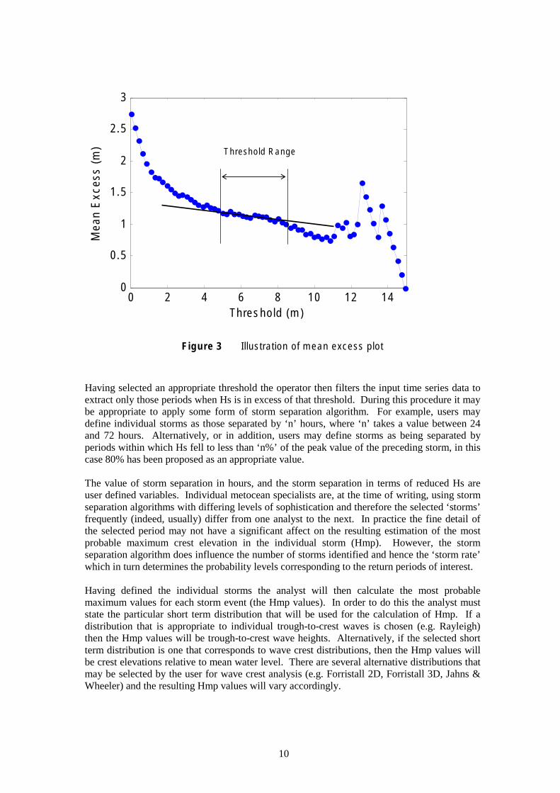
The fist stage in a TVM analysis is therefore to select the threshold that defines storm conditions. A method for doing this based on the ‘mean excess’ is described in the proceedings of OMAE079. Briefly, the mean excess is defined for a long time series of wave data as the average difference between the selected threshold and every Hs value in excess of it. Plotting the mean excess against threshold produces a curve (see Figure 3 that has been extracted from Reference 9).

Plotting the mean excess curve enables the operator to identify the zone within which the mean excess changes linearly with threshold, and it is within this region that the appropriate storm threshold is defined. Tests reported in Reference 9 indicate that an appropriate storm threshold should return approximately 3 events per month when averaged over 12 months.

9 Leggett IM, Bellamy NF, Fox JP and Sheikh R. A Recommended Approach for Deriving ISO-Compliant 10,000 Year Extreme Water Levels in the North Sea 26th International Conference on Offshore Mechanics and Arctic Engineering June 10-15, 2007, San Diego, California. OMAE2007-29559

9

Mea

n E

xces

s (m

) 3

2.5

2

1.5

1

0.5

00 2 4 6 8 10 12 14

lThresho d Range

Threshold (m)

Figure 3 Illustration of mean excess plot

Having selected an appropriate threshold the operator then filters the input time series data to extract only those periods when Hs is in excess of that threshold. During this procedure it may be appropriate to apply some form of storm separation algorithm. For example, users may define individual storms as those separated by ‘n’ hours, where ‘n’ takes a value between 24 and 72 hours. Alternatively, or in addition, users may define storms as being separated by periods within which Hs fell to less than ‘n%’ of the peak value of the preceding storm, in this case 80% has been proposed as an appropriate value.

The value of storm separation in hours, and the storm separation in terms of reduced Hs are user defined variables. Individual metocean specialists are, at the time of writing, using storm separation algorithms with differing levels of sophistication and therefore the selected ‘storms’ frequently (indeed, usually) differ from one analyst to the next. In practice the fine detail of the selected period may not have a significant affect on the resulting estimation of the most probable maximum crest elevation in the individual storm (Hmp). However, the storm separation algorithm does influence the number of storms identified and hence the ‘storm rate’ which in turn determines the probability levels corresponding to the return periods of interest.

Having defined the individual storms the analyst will then calculate the most probable maximum values for each storm event (the Hmp values). In order to do this the analyst must state the particular short term distribution that will be used for the calculation of Hmp. If a distribution that is appropriate to individual trough-to-crest waves is chosen (e.g. Rayleigh) then the Hmp values will be trough-to-crest wave heights. Alternatively, if the selected short term distribution is one that corresponds to wave crest distributions, then the Hmp values will be crest elevations relative to mean water level. There are several alternative distributions that may be selected by the user for wave crest analysis (e.g. Forristall 2D, Forristall 3D, Jahns & Wheeler) and the resulting Hmp values will vary accordingly.

10

Once the Hmp values have been calculated, they must be formed into a frequency distribution prior to extrapolation. Here again there are several options. The unprocessed frequency distribution may be extrapolated, or the data may be classified into class bins prior to extrapolation. In the later case the binning routine tends to add weight to the upper tail and reduce the influence of the lower tail, and the greater the bin size the greater this effect will be.

During the extrapolation of the Hmp data the user may also restrict the fit of the Weibull extrapolation to the upper tail only. So doing excludes any contribution from lower values of Hmp and thus, in effect, reduces the number of storms analysed, and hence the storm rate. Great care should be taken when restricting fits to the upper tail in order to ensure that the storm rate remains valid.

Note also that the parameters of a fit that has been constrained to the upper tail of a distribution do not necessarily provide a fair indication across the entire distribution. Indeed, the parameters of the fitted tail may be significantly in error with respect to regions of that distribution which fall below the tail.

11

4. TIDES

Tides are controlled by the position of celestial bodies, are predictable and are not influenced by weather conditions. In their most simplified approximation, they can be regarded as a sinusoidal wave with a period equal to approximately 12.5 hours. As such, the probability of the tidal level being at its extreme is less than the probability of it being between its extremes (that is to say, the amount of time that the tidal level is actually at high water is relatively small compared with the amount of time the tide is in the process of rising or falling). Figure 4 shows the probability of occurrence of tidal level at the selected study sites, taken from measured data. Note that the area under each of the three lines shown in Figure 4 is equal, and represents a Probability of 1.0.

1.5 1.0 0.5 0.0 0.5 1.0 1.5

Tide (rel msl) [m]

Probability

of Occurance

K13

Euro

Auk

Figure 4 Probability of occurrence of measured tidal level (m) at Auk, K13 and Euro. Relative to MSL

Figure 4 clearly shows that the least likely tidal levels are the extremes (both high and low) while the most likely levels are either side of mean sea level. The shape of the Auk and K13 lines show that at both locations the tide is relatively even in that the time spent above mean sea level is approximately the same as time spent below mean sea level. At Euro, however, the time spent above mean sea level is significantly less than below mean sea level (Probability of being > MSL = 0.45, Probability of being < MSL = 0.55).

While the tides remain un-influenced by the severity of the sea conditions, they can have an influence on them. This is discussed in the next section.

12

4.1 INFLUENCE OF TIDE ON SURGE AND WAVES

It has been reported10 that the tidal level can influence the local surge conditions with greatest effect being felt in shallow waters. This is due to the fact that water depth plays a role in the severity of surges with deeper water lessening the effect of a surge. Thus, in very shallow water, such as the southern North Sea, the tide can alter the water depth sufficiently to alter the surge. However, in deep water, the change in water depth brought about by the tide is slight (as a fraction of the total depth) and so the influence that the tidal level has on surge in deep water will be less.

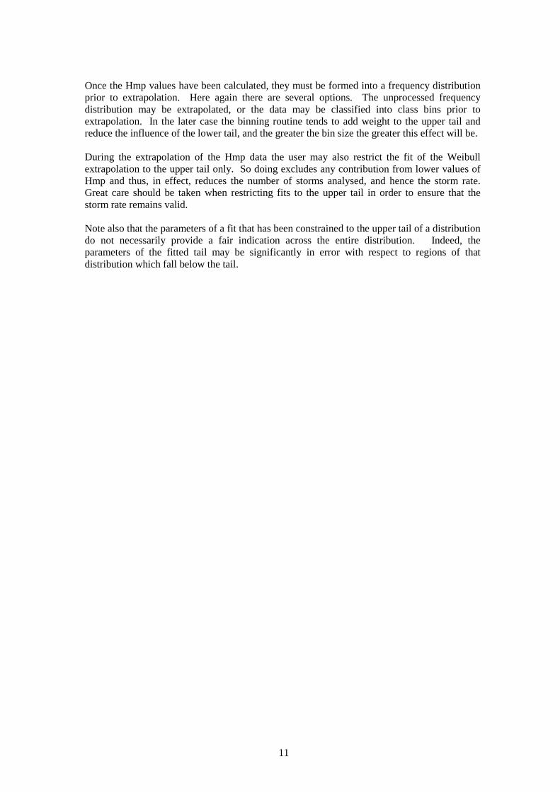
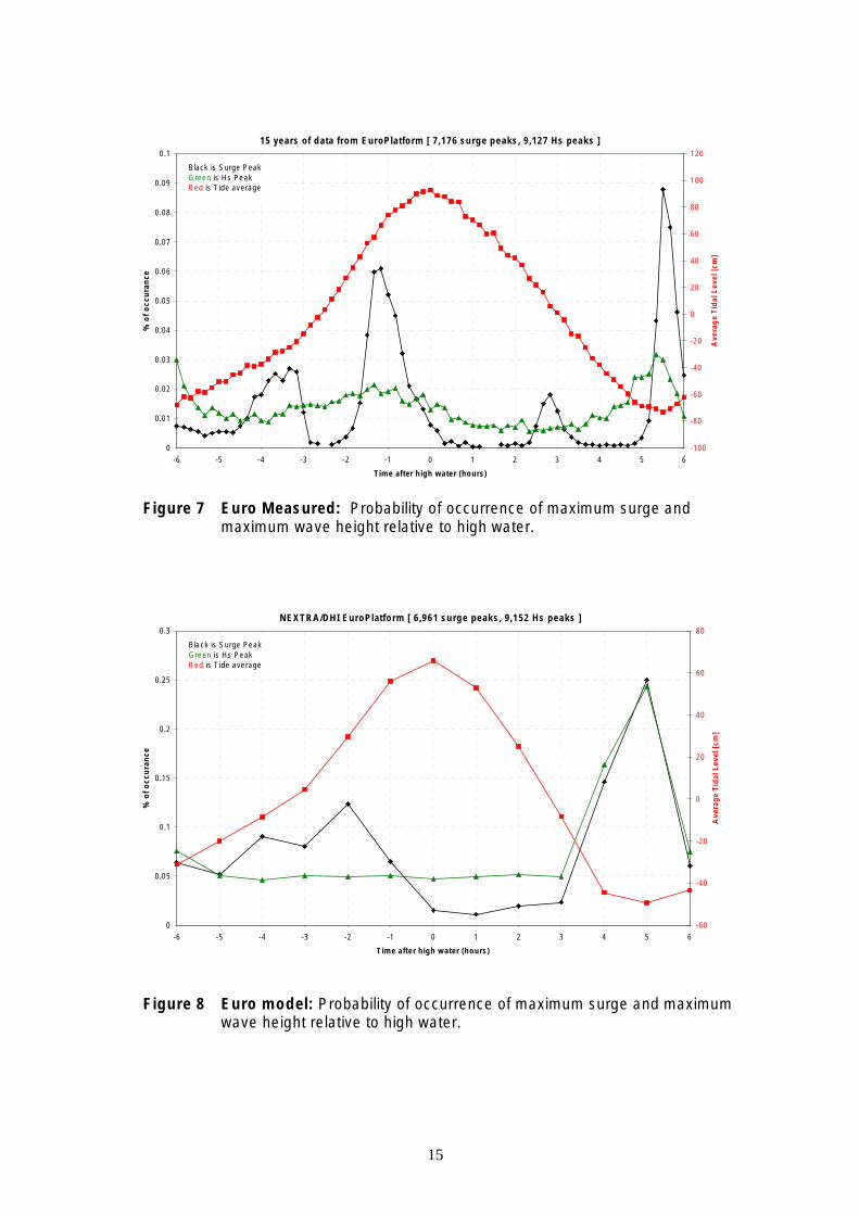
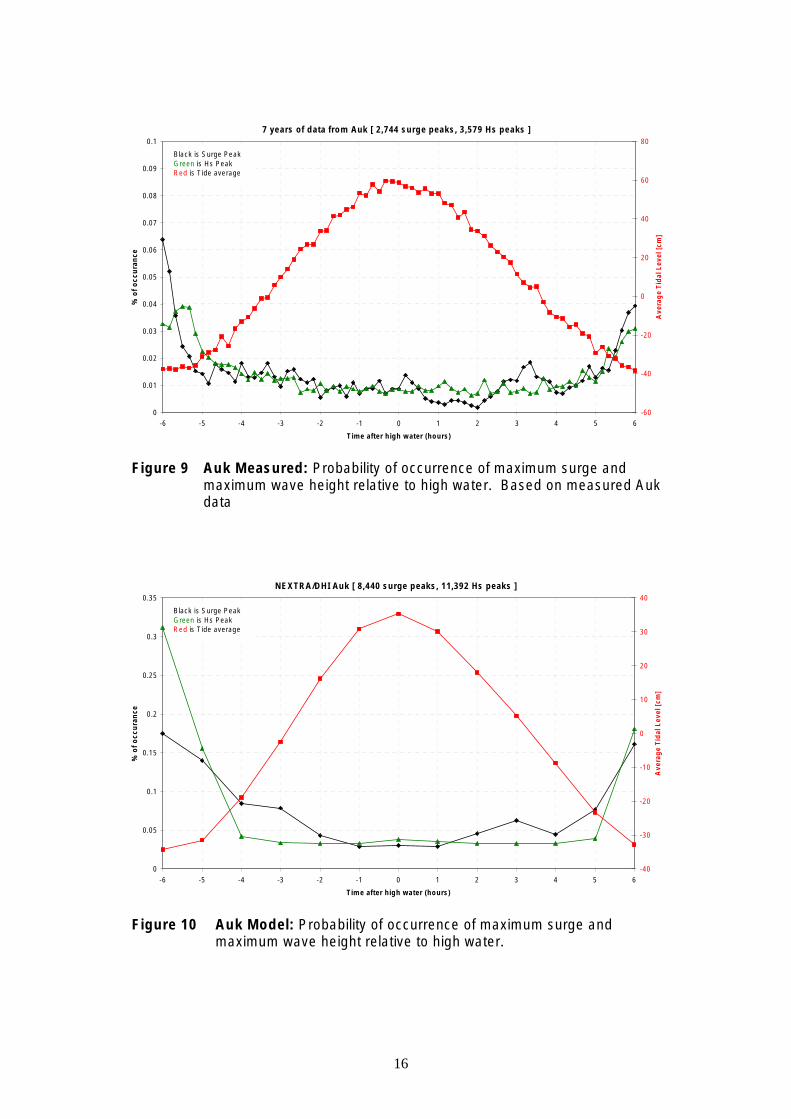
To investigate the influence of tide on surge the data sets were split into tidal cycles, concentrating on the up-tides. For each positive tide (i.e. that part of the tidal cycle when SWL is above MWL) the time of the maximum recorded surge relative to the peak of the tide is recorded. Data were collected for the entire duration of each data set and a probability distribution was created to show when, during the elevated part of the tidal cycle, the maximum surge peak occurred. The task was repeated for the maximum wave height in each positive tide. The results are shown in the Figures 5 to 10. Note that the resolution of the model data is one record every hour whereas the measured data are recorded at 10-minute intervals.

10 Horsburgh K.J. and Wilson C.Tide-surge interaction and its role in the distribution of residuals in the North SeaProudman Oceanographic Laboratory. In press.

13

20 years of data from K13a [ 9,303 surge peaks 11,183 Hs peaks ]

0 0 1 2 3 4 5 6

0

Bl ii

i i

0.01

0.02

0.03

0.04

0.05

0.06

0.07

0.08

0.09

0.1

-6 -5 -4 -3 -2 -1

% o

f occ

ura

nce

-80

-60

-40

-20

20

40

60

80

Ave

rag

e T

idal

Lev

el [

cm]

ack s Surge Peak Green s Hs Peak Red s T de average

Time after high water (hours)

Figure 5 K13 measured: Probability of occurrence of maximum surge and maximum wave height relative to high water.

/

0 0 1 2 3 4 5 6

0

Bl ii

i i

NEXTRA DHI K13a [ 8,031 surge peaks 11,260 Hs peaks ]

0.05

0.1

0.15

0.2

0.25

0.3

0.35

-6 -5 -4 -3 -2 -1

% o

f occ

ura

nce

-150

-100

-50

50

100

150

Ave

rag

e T

idal

Lev

el [

cm]



Figure 6 K13 Model: Probability of occurrence of maximum surge and maximum wave height relative to high water.

14

-6

15 years of data from EuroPlatform [ 7,176 surge peaks, 9,127 Hs peaks ]

0

0

Bl ii

i i

0.01

0.02

0.03

0.04

0.05

0.06

0.07

0.08

0.09

0.1 %

of o

ccu

ran

ce

-100

-80

-60

-40

-20

20

40

60

80

100

120

Ave

rag

e T

idal

Lev

el [

cm]


-5 -4 -3 -2 -1 0 1 2 3 4 5 6


Figure 7 Euro Measured: Probability of occurrence of maximum surge and maximum wave height relative to high water.

NEXTRA/DHI EuroPlatform [ 6,961 surge peaks, 9,152 Hs peaks ]

0

0

Bl ii

i i

0.05

0.1

0.15

0.2

0.25

0.3

% o

f occ

ura

nce

-60

-40

-20

20

40

60

80

Ave

rag

e T

idal

Lev

el [

cm]


-6 -5 -4 -3 -2 -1 0 1 2 3 4 5 6


Figure 8 Euro model: Probability of occurrence of maximum surge and maximum wave height relative to high water.

15

7 years of data from Auk [ 2,744 surge peaks, 3,579 Hs peaks ]

0 0 1 2 3 4 5 6

0

Bl ii

i i

0.01

0.02

0.03

0.04

0.05

0.06

0.07

0.08

0.09

0.1

-6 -5 -4 -3 -2 -1

% o

f occ

ura

nce

-60

-40

-20

20

40

60

80

Ave

rag

e T

idal

Lev

el [

cm]



Figure 9 Auk Measured: Probability of occurrence of maximum surge and maximum wave height relative to high water. Based on measured Auk data

/

0 0 1 2 3 4 5 6

0

Bl ii

i i

NEXTRA DHI Auk [ 8,440 surge peaks, 11,392 Hs peaks ]

0.05

0.1

0.15

0.2

0.25

0.3

0.35

-6 -5 -4 -3 -2 -1

% o

f occ

ura

nce

-40

-30

-20

-10

10

20

30

40

Ave

rag

e T

idal

Lev

el [

cm]



Figure 10 Auk Model: Probability of occurrence of maximum surge and maximum wave height relative to high water.

16

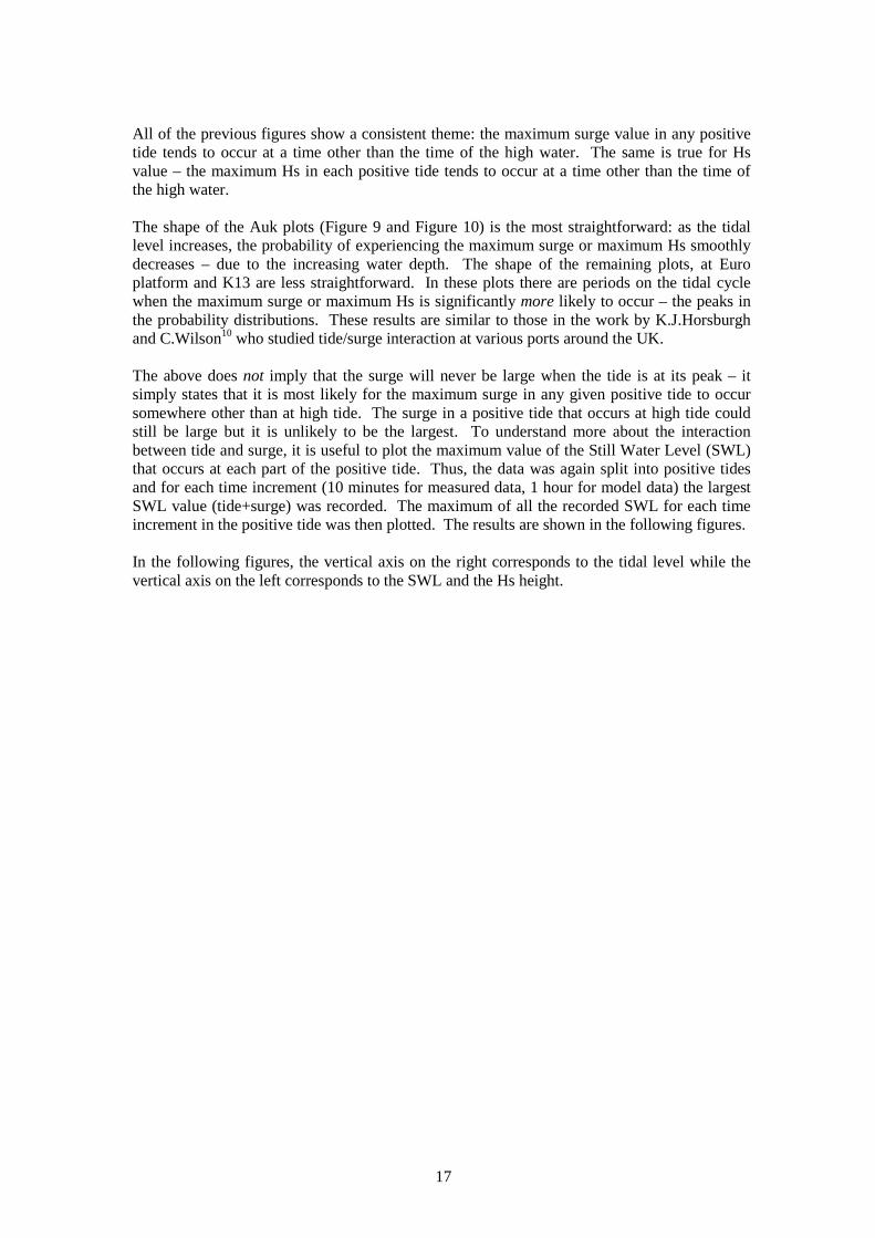
All of the previous figures show a consistent theme: the maximum surge value in any positive tide tends to occur at a time other than the time of the high water. The same is true for Hs value – the maximum Hs in each positive tide tends to occur at a time other than the time of the high water.

The shape of the Auk plots (Figure 9 and Figure 10) is the most straightforward: as the tidal level increases, the probability of experiencing the maximum surge or maximum Hs smoothly decreases – due to the increasing water depth. The shape of the remaining plots, at Euro platform and K13 are less straightforward. In these plots there are periods on the tidal cycle when the maximum surge or maximum Hs is significantly more likely to occur – the peaks in the probability distributions. These results are similar to those in the work by K.J.Horsburgh and C.Wilson10 who studied tide/surge interaction at various ports around the UK.

The above does not imply that the surge will never be large when the tide is at its peak – it simply states that it is most likely for the maximum surge in any given positive tide to occur somewhere other than at high tide. The surge in a positive tide that occurs at high tide could still be large but it is unlikely to be the largest. To understand more about the interaction between tide and surge, it is useful to plot the maximum value of the Still Water Level (SWL) that occurs at each part of the positive tide. Thus, the data was again split into positive tides and for each time increment (10 minutes for measured data, 1 hour for model data) the largest SWL value (tide+surge) was recorded. The maximum of all the recorded SWL for each time increment in the positive tide was then plotted. The results are shown in the following figures.

In the following figures, the vertical axis on the right corresponds to the tidal level while the vertical axis on the left corresponds to the SWL and the Hs height.

17

7 years of data from Auk [ 2,744 surge peaks, 3,579 Hs peaks ]

0 0 1 2 3 4 5 6

0

Bl ii

i i

200

400

600

800

1000

1200

1400

-6 -5 -4 -3 -2 -1

Lev

el (

cm)

-60

-40

-20

20

40

60

80

Ave

rag

e T

idal

Lev

el (

cm)

ack s SWL Peak Green s Hs Peak Red s T de average


Figure 11 Auk Measured: Maximum Hs and SWL throughout the positive tide.

/

0 0 1 2 3 4 5 6

0

Bl ii

i i

NEXTRA DHI Auk [ 8,440 surge peaks, 11,392 Hs peaks ]

200

400

600

800

1000

1200

1400

-6 -5 -4 -3 -2 -1

Lev

el (

cm)

-40

-30

-20

-10

10

20

30

40

Ave

rag

e T

idal

Lev

el (

cm)



Figure 12 Auk Model: Maximum Hs and SWL throughout the positive tide.

18

20 years of data from K13a [ 9,303 surge peaks 11,183 Hs peaks ]

0 0 1 2 3 4 5 6

0

Bl ii

i i

100

200

300

400

500

600

700

800

900

-6 -5 -4 -3 -2 -1

Lev

el (

cm)

-80

-60

-40

-20

20

40

60

80

Ave

rag

e T

idal

Lev

el (

cm)



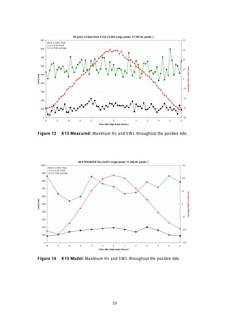
Figure 13 K13 Measured: Maximum Hs and SWL throughout the positive tide.

/

0 0 1 2 3 4 5 6

0

Bl ii

i i

NEXTRA DHI K13a [ 8,031 surge peaks 11,260 Hs peaks ]

100

200

300

400

500

600

700

800

900

1000

-6 -5 -4 -3 -2 -1

Lev

el (

cm)

-150

-100

-50

50

100

150

Ave

rag

e T

idal

Lev

el (

cm)



Figure 14 K13 Model: Maximum Hs and SWL throughout the positive tide.

19

15 years of 10 minute data from EuroPlatform [ 7,176 surge peaks, 9,127 Hs peaks ]

0 0 1 2 3 4 5 6

0

Bl ii

i i

100

200

300

400

500

600

700

-6 -5 -4 -3 -2 -1

Lev

el (

cm)

-100

-80

-60

-40

-20

20

40

60

80

100

120

Ave

rag

e T

idal

Lev

el (

cm)



Figure 15 Euro Measured: Maximum Hs and SWL throughout the positive tide.

/

0

0

Bl ii

i i

NEXTRA DHI EuroPlatform [ 6,961 surge peaks, 9,152 Hs peaks ]

100

200

300

400

500

600

700

800

Lev

el (

cm)

-60

-40

-20

20

40

60

80

Ave

rag

e T

idal

Lev

el (

cm)


-6 -5 -4 -3 -2 -1 0 1 2 3 4 5 6


Figure 16 Euro Model: Maximum Hs and SWL throughout the positive tide.

20

The preceding plots are based on extracting maxima – hence they will be rather noisy. However, the trend is the same across all the plots – the maximum Hs and maximum surge values appear to be independent of tidal level. If the tide had no influence on the surge then the maximum surge would be equally likely to occur at any point on the tidal cycle and therefore the maximum SWL (which is the sum of the maximum surge and the tidal level) would have approximately the same shape as the tidal level. The preceding plots show that this is not the case; in fact the SWL is relatively constant across the positive tide indicating that the tide and the surge interact with the tide effectively moderating the effect of the surge such that the maximum SWL is unvarying.

This is emphasized by the data contained in Table 1 which shows that the maximum surge from the three study sites actually occurred when the tide was negative and that the maximum SWL comprises neither the maximum surge nor the maximum tidal level. Furthermore, the maximum Hs values in all the data sets occurred at moderate tidal levels (all less than 54 % of the maximum tide).

5. STORMS

The previous section has shown that tides can, and do, have an effect on when the largest Hs and surge are most likely to occur in a tidal cycle. However, as will be shown in this section, a storm can last much longer than a complete tidal cycle and so while the tides may affect when the largest surge value occurs within a tidal cycle, it is true to say that the surge can be large for long periods of time – sometimes the surge remains large over many complete tidal cycles.

5.1 SURGE DURATION

To investigate the duration of storms, the surges were analysed and the duration which the surge level persisted above a given threshold was recorded. The threshold was varied from 0 cm to 100 cm in increments of 10 cm. The following figures present the results of the surge durations analysis.

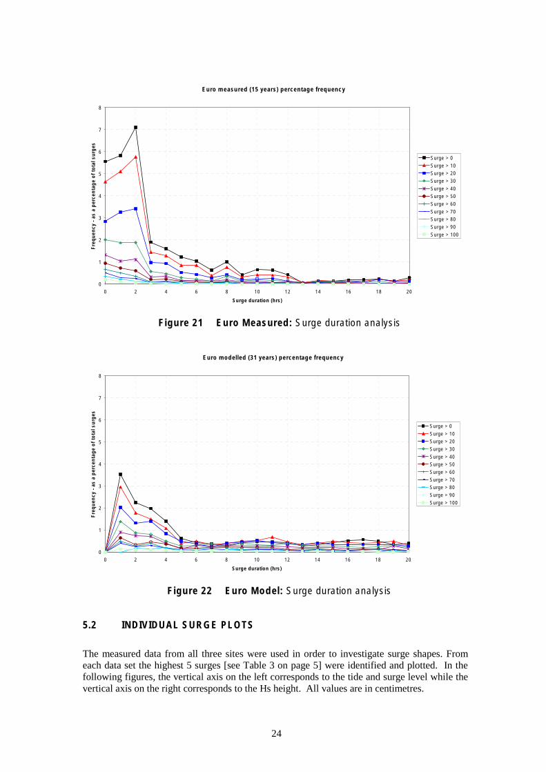
Figures 17 to 22 show that while the majority of surges are relatively short (less than around 6 hours) there are still surges, both small and large, which persist for a considerable time. To understand the duration and shape of the storm surges, the top 5 surges were extracted from each data set and plotted. The plots and the discussion appear after Figure 22.

21

Auk measured (7 years) percentage frequency F

req

uen

cy a

s a

per

cen

tag

e o

f to

tal s

urg

es

Fre

qu

ency

as

a p

erce

nta

ge

of

tota

l su

rges

0

2

4

6

8

0 2 4 6 8

10

12

14

16

18

20

10 12 14 16 18 20

Surge > 0

Surge > 10

Surge > 20

Surge > 30

Surge > 40

Surge > 50

Surge > 60

Surge > 70

Surge > 80

Surge > 90

Surge > 100

Surge duration (hrs)

Figure 17 Auk Measured: Surge duration analysis

Auk modelled (31 years) percentage frequency

0

2

4

6

8

10

12

14

16

18

20

Surge > 0

Surge > 10

Surge > 20

Surge > 30

Surge > 40

Surge > 50

Surge > 60

Surge > 70

Surge > 80

Surge > 90

Surge > 100

0 2 4 6 8 10 12 14 16 18 20


Figure 18 Auk Model: Surge duration analysis

22

K13 Measured (20 years) percentage frequency F

req

uen

cy -

as a

per

cen

tag

e o

f to

tal s

urg

es

Fre

qu

ency

-as

a p

erce

nta

ge

of

tota

l su

rges

0

1

2

3

4

5

6

7

8

9

0 2 4 6 8

10

10 12 14 16 18 20

Surge > 0

Surge > 10

Surge > 20

Surge > 30

Surge > 40

Surge > 50

Surge > 60

Surge > 70

Surge > 80

Surge > 90

Surge > 100


Figure 19 K13 Measured: Surge duration analysis

K13 Modelled (31 years) percentage frequency

0

1

2

3

4

5

6

7

8

9

10

Surge > 0

Surge > 10

Surge > 20

Surge > 30

Surge > 40

Surge > 50

Surge > 60

Surge > 70

Surge > 80

Surge > 90

Surge > 100

0 2 4 6 8 10 12 14 16 18 20


Figure 20 K13 Model: Surge duration analysis based on model K13 data

23

Euro measured (15 years) percentage frequency

0

1

2

3

4

5

6

7

8

Fre

qu

ency

-as

a p

erce

nta

ge

of

tota

l su

rges

Surge > 0

Surge > 10

Surge > 20

Surge > 30

Surge > 40

Surge > 50

Surge > 60

Surge > 70

Surge > 80

Surge > 90

Surge > 100

0 2 4 6 8 10 12 14 16 18 20


Figure 21 Euro Measured: Surge duration analysis

Euro modelled (31 years) percentage frequency

0

1

2

3

4

5

6

7

8

Fre

qu

ency

-as

a p

erce

nta

ge

of

tota

l su

rges

Surge > 0

Surge > 10

Surge > 20

Surge > 30

Surge > 40

Surge > 50

Surge > 60

Surge > 70

Surge > 80

Surge > 90

Surge > 100

0 2 4 6 8 10 12 14 16 18 20


Figure 22 Euro Model: Surge duration analysis

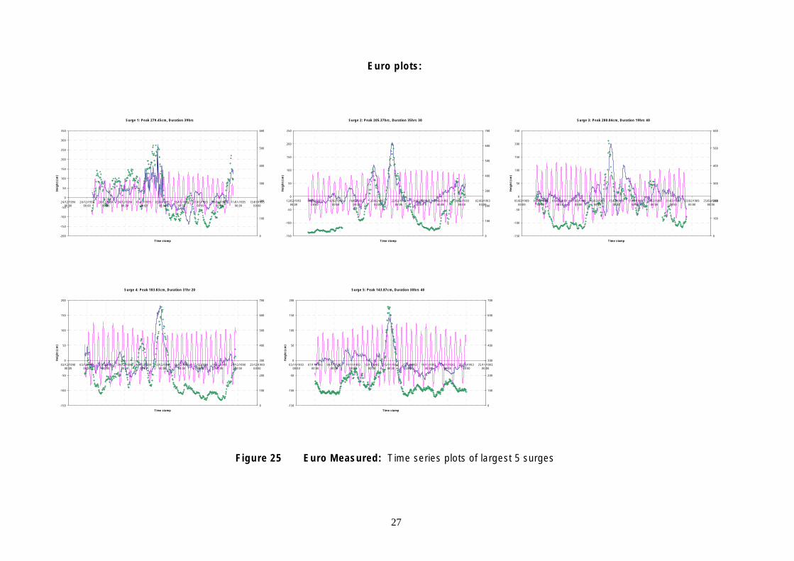
5.2 INDIVIDUAL SURGE PLOTS

The measured data from all three sites were used in order to investigate surge shapes. From each data set the highest 5 surges [see Table 3 on page 5] were identified and plotted. In the following figures, the vertical axis on the left corresponds to the tide and surge level while the vertical axis on the right corresponds to the Hs height. All values are in centimetres.

24

25

Auk plots:

Surge 1: Peak 212.59cm, Duration 139 hrs

-100

-50

0

50

100

150

200

250

18/02/199000:00

20/02/199000:00

22/02/199000:00

24/02/199000:00

26/02/199000:00

28/02/199000:00

02/03/199000:00

04/03/199000:00

06/03/199000:00

08/03/199000:00

10/03/199000:00

Time stamp

Hei

gh

t (c

m)

0

100

200

300

400

500

600

700

800

900

Surge 2: Peak 189.3cm, Duration 118hr 10min

-100

-50

0

50

100

150

200

250

10/09/199000:00

12/09/199000:00

14/09/199000:00

16/09/199000:00

18/09/199000:00

20/09/199000:00

22/09/199000:00

24/09/199000:00

26/09/199000:00

28/09/199000:00

30/09/199000:00

Time stamp

Hei

gh

t (c

m)

0

100

200

300

400

500

600

700

800

900

Surge 3: Peak 184.81cm, Duration 93hrs 50

-100

-50

0

50

100

150

200

12/02/199300:00

14/02/199300:00

16/02/199300:00

18/02/199300:00

20/02/199300:00

22/02/199300:00

24/02/199300:00

26/02/199300:00

28/02/199300:00

02/03/199300:00

Time stamp

Hei

gh

t (c

m)

0

200

400

600

800

1000

1200

Surge 4: Peak 178.73cm, Duration 50hrs

-100

-50

0

50

100

150

200

09/10/199100:00

11/10/199100:00

13/10/199100:00

15/10/199100:00

17/10/199100:00

19/10/199100:00

21/10/199100:00

23/10/199100:00

25/10/199100:00

27/10/199100:00

29/10/199100:00

Time stamp

Hei

gh

t (c

m)

0

200

400

600

800

1000

1200


-100

-50

0

50

100

150

200

03/12/199000:00

05/12/199000:00

07/12/199000:00

09/12/199000:00

11/12/199000:00

13/12/199000:00

15/12/199000:00

17/12/199000:00

19/12/199000:00

21/12/199000:00

23/12/199000:00

Time stamp

Hei

gh

t (c

m)

0

200

400

600

800

1000

1200

1400

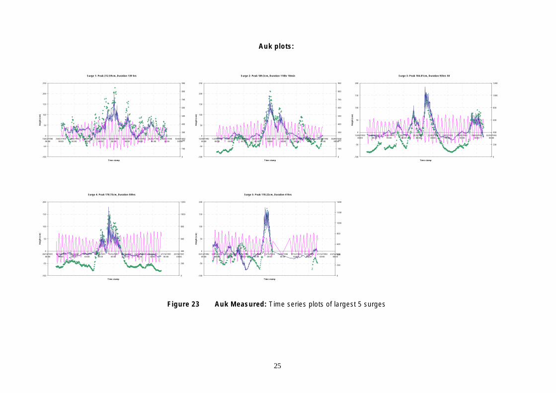
Figure 23 Auk Measured: Time series plots of largest 5 surges

26

K13 Plots:


-100

-50

0

50

100

150

200

250

10/12/199100:00

12/12/199100:00

14/12/199100:00

16/12/199100:00

18/12/199100:00

20/12/199100:00

22/12/199100:00

24/12/199100:00

26/12/199100:00

28/12/199100:00

30/12/199100:00

Time Stamp

Hei

gh

t (c

m)

0

100

200

300

400

500

600


-100

-50

0

50

100

150

200

250

12/02/199300:00

14/02/199300:00

16/02/199300:00

18/02/199300:00

20/02/199300:00

22/02/199300:00

24/02/199300:00

26/02/199300:00

28/02/199300:00

02/03/199300:00

Time stamp

Hei

gh

t (c

m)

0

100

200

300

400

500

600

700

800


-150

-100

-50

0

50

100

150

200

09/10/199100:00

11/10/199100:00

13/10/199100:00

15/10/199100:00

17/10/199100:00

19/10/199100:00

21/10/199100:00

23/10/199100:00

25/10/199100:00

27/10/199100:00

29/10/199100:00

Time stamp

Hei

gh

t (c

m)

0

100

200

300

400

500

600

700


-100

-50

0

50

100

150

200

05/02/198900:00

07/02/198900:00

09/02/198900:00

11/02/198900:00

13/02/198900:00

15/02/198900:00

17/02/198900:00

19/02/198900:00

21/02/198900:00

23/02/198900:00

25/02/198900:00

Time stamp

Hei

gh

t (c

m)


-100

-50

0

50

100

150

200

03/12/199000:00

05/12/199000:00

07/12/199000:00

09/12/199000:00

11/12/199000:00

13/12/199000:00

15/12/199000:00

17/12/199000:00

19/12/199000:00

21/12/199000:00

23/12/199000:00

Time stamp

Hei

gh

t (c

m)

0

100

200

300

400

500

600

700

800

900

No Hs data available during above storm

Figure 24 K13 Measured: Time series plots of largest 5 surges

27

Euro plots:


-200

-150

-100

-50

0

50

100

150

200

250

300

350

24/12/199400:00

26/12/199400:00

28/12/199400:00

30/12/199400:00

01/01/199500:00

03/01/199500:00

05/01/199500:00

07/01/199500:00

09/01/199500:00

11/01/199500:00

13/01/199500:00

Time stamp

Hei

gh

t (c

m)

0

100

200

300

400

500

600

Surge 2: Peak 205.37hrs, Duration 35hrs 30

-150

-100

-50

0

50

100

150

200

250

12/02/199300:00

14/02/199300:00

16/02/199300:00

18/02/199300:00

20/02/199300:00

22/02/199300:00

24/02/199300:00

26/02/199300:00

28/02/199300:00

02/03/199300:00

Time stamp

Hei

gh

t (c

m)

0

100

200

300

400

500

600

700


-150

-100

-50

0

50

100

150

200

250

05/02/198900:00

07/02/198900:00

09/02/198900:00

11/02/198900:00

13/02/198900:00

15/02/198900:00

17/02/198900:00

19/02/198900:00

21/02/198900:00

23/02/198900:00

25/02/198900:00

Time stamp

Hei

gh

t (c

m)

0

100

200

300

400

500

600

Surge 4: Peak 183.83cm, Duration 31hr 20

-150

-100

-50

0

50

100

150

200

03/12/199000:00

05/12/199000:00

07/12/199000:00

09/12/199000:00

11/12/199000:00

13/12/199000:00

15/12/199000:00

17/12/199000:00

19/12/199000:00

21/12/199000:00

23/12/199000:00

Time stamp

Hei

gh

t (c

m)

0

100

200

300

400

500

600

700


-150

-100

-50

0

50

100

150

200

05/11/199300:00

07/11/199300:00

09/11/199300:00

11/11/199300:00

13/11/199300:00

15/11/199300:00

17/11/199300:00

19/11/199300:00

21/11/199300:00

23/11/199300:00

25/11/199300:00

Time stamp

Hei

gh

t (c

m)

0

100

200

300

400

500

600

700

Figure 25 Euro Measured: Time series plots of largest 5 surges

Table 3 Height and Duration of the 5 largest Surges at Auk, K13 and Euro

Surge Peak Height [m] Surge Peak Duration [hours]

Auk K13 Euro Auk K13 Euro

Surge 1 2.13 1.98 2.79 139 123 39

Surge 2 1.89 1.97 2.05 118 38 36

Surge 3 1.84 1.77 2.00 94 93 20

Surge 4 1.78 1.73 1.84 50 20 31

Surge 5 1.78 1.65 1.44 41 29 31

Figures 23 to 25 show that large surges and large Hs values are generally coincident – although as shown earlier in Table 1 on page 5, the maximum surge is not coincident with the maximum Hs. They also show that large surges can persist for considerable times – occasionally measurable in days. In terms of extreme water level, the previous plots are relevant in that they show that large Hs values should be accompanied by large surges, but that the relationship is not linear because the largest surge does not coincide with the largest Hs.

To further investigate the relationship between Hs and surge, scatter plots of Hs and surge were generated for the 3 locations. These are shown in the following section.

28

6. RELATIONSHIP BETWEEN SURGE AND WAVE HEIGHT

In this section, the relationship between surge and wave height is examined. For each location, the positive surges were plotted against the wave height to create a scatter plot. If the relationship between surge height and wave height were linear, one would expect to see a scatter of points lying approximately on a line of constant gradient of 1. However, as the following plots show, the relationship between surge and wave height is not a simple linear relationship. [Note that there was no appreciable difference in the shape of the plots when using measured or model data and so, for brevity, only the measured data plots are included below].

In the less shallow waters at Auk (85 m depth), the surges remain small for larger values of wave height than at Euro platforms or K13, as seen in Figure 26. However, large wave heights are not necessarily associated with large surges.

Figure 27 shows that, at K13, as the wave height (labeled as H4RM0 on the x-axis) increases, the surge also increases. However, for any given wave height, there are many instances of surges below the maximum surge for that wave height. Thus, a large wave height does not automatically imply that the surge will be large. Even when the waves are particularly severe – say 7 m – surges still occur which are very small. Experiencing a large wave does not automatically mean that the surge will be large.

At the Euro platform, Figure 28, the situation is very similar to that of K13 with the largest wave heights having associated surges which are distributed across the range of surge values.

In summary, the degree of association between wave height and surge is not straightforward and is affected by location (depth). In general, as the wave height increases, the range of surges that can be associated with the wave also increase but it does not follow that large waves are associated with only large surges.

29

Figure 26 Auk Measured: Hs-Surge (positive only) scatter plot

Figure 27 K13 Measured: Hs-Surge (positive only) scatter plot

Figure 28 Euro Measured: Hs-Surge (positive only) scatter plot

30

7. MONTE CARLO SIMULATIONS

Whilst it is possible to convolve two distributions mathematically, the task becomes increasingly complex as more distributions are involved. In such cases Monte Carlo simulation (named after a location famous for its games of chance) is a recognized technique. In broad terms, to perform a Monte Carlo simulation one has to define each of the input parameters in terms of its frequency distribution. Sequential random selections are then made from the several distributions describing each input parameter in order to construct a new distribution that represents all parameters acting in combination. This is relatively easy when the input parameters are entirely independent of each-other, but special attention must be given to partially dependent parameters such as, in this case, wave and surge.

Measured data sets are, at best, only tens of years in duration. This is sufficient to identify the distributions of wave height, tide and surge and, by using Monte Carlo methods, longer durations can be simulated.

A Monte Carlo method has been adopted in order to convolve the short and long term distributions of waves, the tidal and surge signals. After a brief description of the software, the results of the study are presented and discussed.

7.1 THE PROCESS

Each analysis consists of multiple individual simulations, each being run over a number of years. For example, to extract statistics for 100 years one would perform a simulation of 100 years duration and repeat the simulation, say, 1,000 times – thus the 100 year statistics would be based on 1,000 entries. The more repetitions of a simulated period, the smoother the resulting frequency distribution (such as that plotted in Figure 2) and the more reliable will be the statistics.

7.1.1 Wave heights

The Monte Carlo simulation process works by randomly choosing Hs values for all the sea states within the specified duration of the simulation. For the particular application under consideration, the specified duration is normally the return period for which extreme values are required (100 or 10,000 years). The Hs values are chosen at random from the Hs distribution which is entered by the user in terms of the scale, shape and location parameters of the selected distribution. If a single Hs distribution is used then all the sea state Hs values are chosen at random from a Weibull distribution.

A multiple wave distribution option has been built into the software for this process. This provides the option of ensuring that the distribution of sea states is not perfectly described by any one function. If multiple distributions (of which there are 4: Weibull, Fisher-Tippett Type 1, Fisher-Tippett Type 3 and Exponential) are used then the distribution from which the sea state will be drawn is first chosen at random and then the Hs is chosen at random from the selected distribution.

31

The chosen Hs for a sea state is then used, in conjunction with the (fixed) Tz or steepness11 to determine how many wave crests occur in that sea state.

The correct number of crests are then chosen, at random, from a distribution of crests based on Hs, Tz, depth using either the Forristall 2D, Forristall 3D or Rayleigh crest distribution (user selectable).

The various options are entered via the input screen, as illustrated in Figure 29.

Figure 29 Monte Carlo: Input Specifications for Significant Wave Height

11 Steepness is defined as 1/S = (2*π*Hs) / (9.81*Tz^2)

32

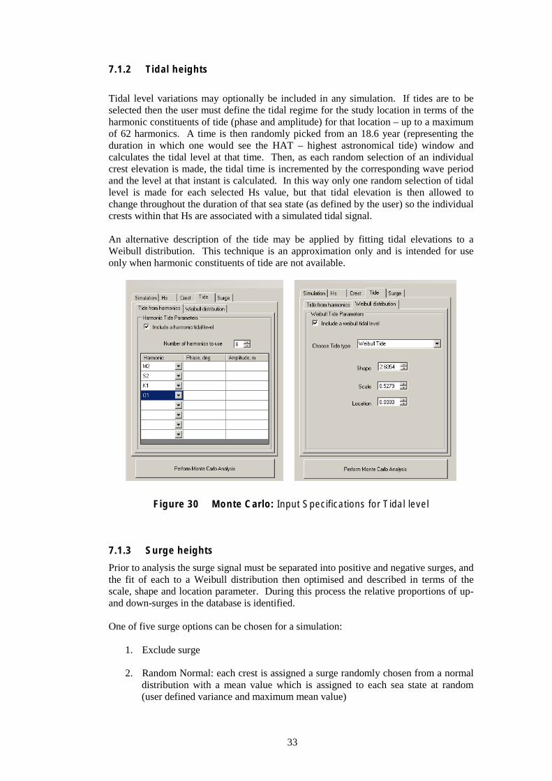
7.1.2 Tidal heights

Tidal level variations may optionally be included in any simulation. If tides are to be selected then the user must define the tidal regime for the study location in terms of the harmonic constituents of tide (phase and amplitude) for that location – up to a maximum of 62 harmonics. A time is then randomly picked from an 18.6 year (representing the duration in which one would see the HAT – highest astronomical tide) window and calculates the tidal level at that time. Then, as each random selection of an individual crest elevation is made, the tidal time is incremented by the corresponding wave period and the level at that instant is calculated. In this way only one random selection of tidal level is made for each selected Hs value, but that tidal elevation is then allowed to change throughout the duration of that sea state (as defined by the user) so the individual crests within that Hs are associated with a simulated tidal signal.

An alternative description of the tide may be applied by fitting tidal elevations to a Weibull distribution. This technique is an approximation only and is intended for use only when harmonic constituents of tide are not available.

Figure 30 Monte Carlo: Input Specifications for Tidal level

7.1.3 Surge heights

Prior to analysis the surge signal must be separated into positive and negative surges, and the fit of each to a Weibull distribution then optimised and described in terms of the scale, shape and location parameter. During this process the relative proportions of up-and down-surges in the database is identified.

One of five surge options can be chosen for a simulation:

1. Exclude surge

2. Random Normal: each crest is assigned a surge randomly chosen from a normal distribution with a mean value which is assigned to each sea state at random (user defined variance and maximum mean value)

33

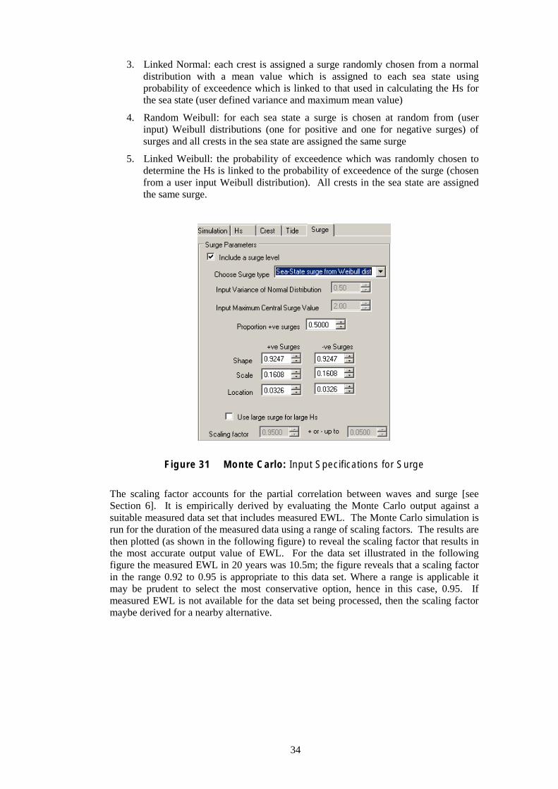
3. Linked Normal: each crest is assigned a surge randomly chosen from a normal distribution with a mean value which is assigned to each sea state using probability of exceedence which is linked to that used in calculating the Hs for the sea state (user defined variance and maximum mean value)

4. Random Weibull: for each sea state a surge is chosen at random from (user input) Weibull distributions (one for positive and one for negative surges) of surges and all crests in the sea state are assigned the same surge

5. Linked Weibull: the probability of exceedence which was randomly chosen to determine the Hs is linked to the probability of exceedence of the surge (chosen from a user input Weibull distribution). All crests in the sea state are assigned the same surge.

Figure 31 Monte Carlo: Input Specifications for Surge

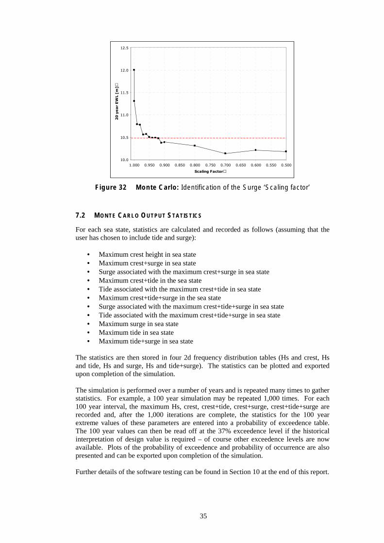
The scaling factor accounts for the partial correlation between waves and surge [see Section 6]. It is empirically derived by evaluating the Monte Carlo output against a suitable measured data set that includes measured EWL. The Monte Carlo simulation is run for the duration of the measured data using a range of scaling factors. The results are then plotted (as shown in the following figure) to reveal the scaling factor that results in the most accurate output value of EWL. For the data set illustrated in the following figure the measured EWL in 20 years was 10.5m; the figure reveals that a scaling factor in the range 0.92 to 0.95 is appropriate to this data set. Where a range is applicable it may be prudent to select the most conservative option, hence in this case, 0.95. If measured EWL is not available for the data set being processed, then the scaling factor maybe derived for a nearby alternative.

34

10.0

10.5

11.0

11.5

12.0

12.5

0.500 0.550 0.600 0.650 0.700 0.750 0.800 0.850 0.900 0.950 1.000

Scaling Factor

20yearEWL[m]

Figure 32 Monte Carlo: Identification of the Surge ‘Scaling factor’

7.2 MONTE CARLO OUTPUT STATISTICS

For each sea state, statistics are calculated and recorded as follows (assuming that the user has chosen to include tide and surge):

• Maximum crest height in sea state • Maximum crest+surge in sea state • Surge associated with the maximum crest+surge in sea state • Maximum crest+tide in the sea state • Tide associated with the maximum crest+tide in sea state • Maximum crest+tide+surge in the sea state • Surge associated with the maximum crest+tide+surge in sea state • Tide associated with the maximum crest+tide+surge in sea state • Maximum surge in sea state • Maximum tide in sea state • Maximum tide+surge in sea state

The statistics are then stored in four 2d frequency distribution tables (Hs and crest, Hs and tide, Hs and surge, Hs and tide+surge). The statistics can be plotted and exported upon completion of the simulation.

The simulation is performed over a number of years and is repeated many times to gather statistics. For example, a 100 year simulation may be repeated 1,000 times. For each 100 year interval, the maximum Hs, crest, crest+tide, crest+surge, crest+tide+surge are recorded and, after the 1,000 iterations are complete, the statistics for the 100 year extreme values of these parameters are entered into a probability of exceedence table. The 100 year values can then be read off at the 37% exceedence level if the historical interpretation of design value is required – of course other exceedence levels are now available. Plots of the probability of exceedence and probability of occurrence are also presented and can be exported upon completion of the simulation.

Further details of the software testing can be found in Section 10 at the end of this report.

35

8. RESULTS

Simulations of 100 and 10,000 years were performed for each of the three locations. Each simulation was repeated 600 times to acquire reliable statistics. The simulation inputs for the distribution of Hs and surge were found by fitting a Weibull 3-parameter distribution to the measured Hs and surge data from each location (the data was sub-sampled to 3 hours so that the number of surge entries matched the number of Hs entries).

‘Worst case’ scenario simulations were run whereby the Hs and surge were linked such that the surge that accompanied each Hs had the same probability of exceedence as the Hs – this is equivalent to combining the n-year Hs with the n-year surge, for example.. The results from these simulations were compared with existing extreme water level methods.

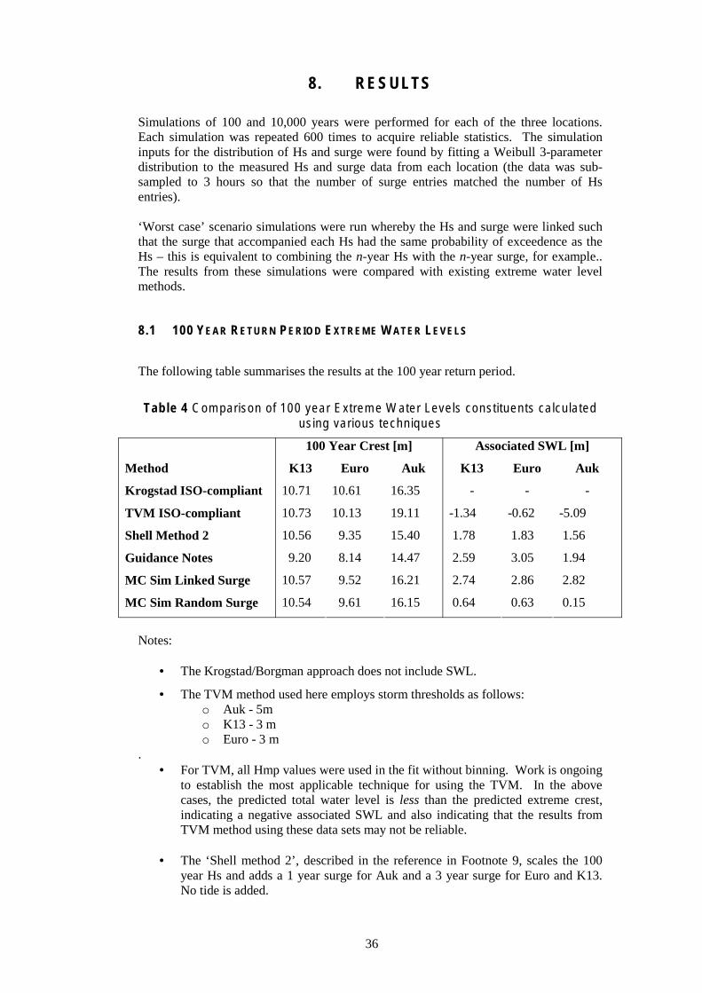
8.1 100 YEAR RETURN PERIOD EXTREME WATER LEVELS

The following table summarises the results at the 100 year return period.

Table 4 Comparison of 100 year Extreme Water Levels constituents calculated using various techniques

100 Year Crest [m] Associated SWL [m]

Method K13 Euro Auk K13 Euro Auk

Krogstad ISO-compliant 10.71 10.61 16.35 - - -

TVM ISO-compliant 10.73 10.13 19.11 -1.34 -0.62 -5.09

Shell Method 2 10.56 9.35 15.40 1.78 1.83 1.56

Guidance Notes 9.20 8.14 14.47 2.59 3.05 1.94

MC Sim Linked Surge 10.57 9.52 16.21 2.74 2.86 2.82

MC Sim Random Surge 10.54 9.61 16.15 0.64 0.63 0.15

Notes:

• The Krogstad/Borgman approach does not include SWL.

• The TVM method used here employs storm thresholds as follows: o Auk - 5m o K13 - 3 m o Euro - 3 m

. • For TVM, all Hmp values were used in the fit without binning. Work is ongoing

to establish the most applicable technique for using the TVM. In the above cases, the predicted total water level is less than the predicted extreme crest, indicating a negative associated SWL and also indicating that the results from TVM method using these data sets may not be reliable.

• The ‘Shell method 2’, described in the reference in Footnote 9, scales the 100 year Hs and adds a 1 year surge for Auk and a 3 year surge for Euro and K13. No tide is added.

36

• The method described in footnote 2, commonly referred to within the oil and gas industry as the ‘Guidance Notes’ method is found by scaling the 50 year Hs and using SWL values from the guidance notes using nearest standard port data

• The MC simulations used either a random or linked surge from the Weibull distributions and a tide value equal to the largest tide from each measured data set.

The 100 year extreme water levels, relative to mean sea level, are as follows:

Table 5 Summary of 100 year Extreme Water Levels found using different techniques

100 Year Total Water Level [m]

Method K13 Euro Auk

TVM ISO-compliant 9.39 9.51 14.02

Shell Method 2 12.34 11.18 16.96

Guidance Notes 11.79 11.19 16.41

MC Sim Linked Surge 13.31 12.38 19.03

MC Sim Random Surge 11.18 10.24 16.30

8.2 10,000 YEAR RETURN PERIOD EXTREME WATER LEVELS

The following table summarises the results at the 10,000 year return period.

Table 6 Comparison of 100 year Extreme Water Levels constituents calculated using various techniques

10,000 Year Crest [m] Associated SWL [m]

Method K13 Euro Auk K13 Euro Auk

Krogstad ISO-compliant 13.96 14.38 21.36 - - -

TVM ISO-compliant 14.66 14.24 28.78 -3.31 -2.65 -11.34

Shell Method 2 14.21 12.58 19.88 1.78 1.83 1.56

Guidance Notes 12.10 10.71 19.03 2.92 3.44 2.19

Shell Method 1 11.48 10.69 17.63 2.00 2.29 2.01

MC Sim Linked Surge 13.92 12.75 21.36 3.50 3.70 4.18

MC Sim Random Surge 13.88 12.79 21.16 0.52 0.56 0.34

37

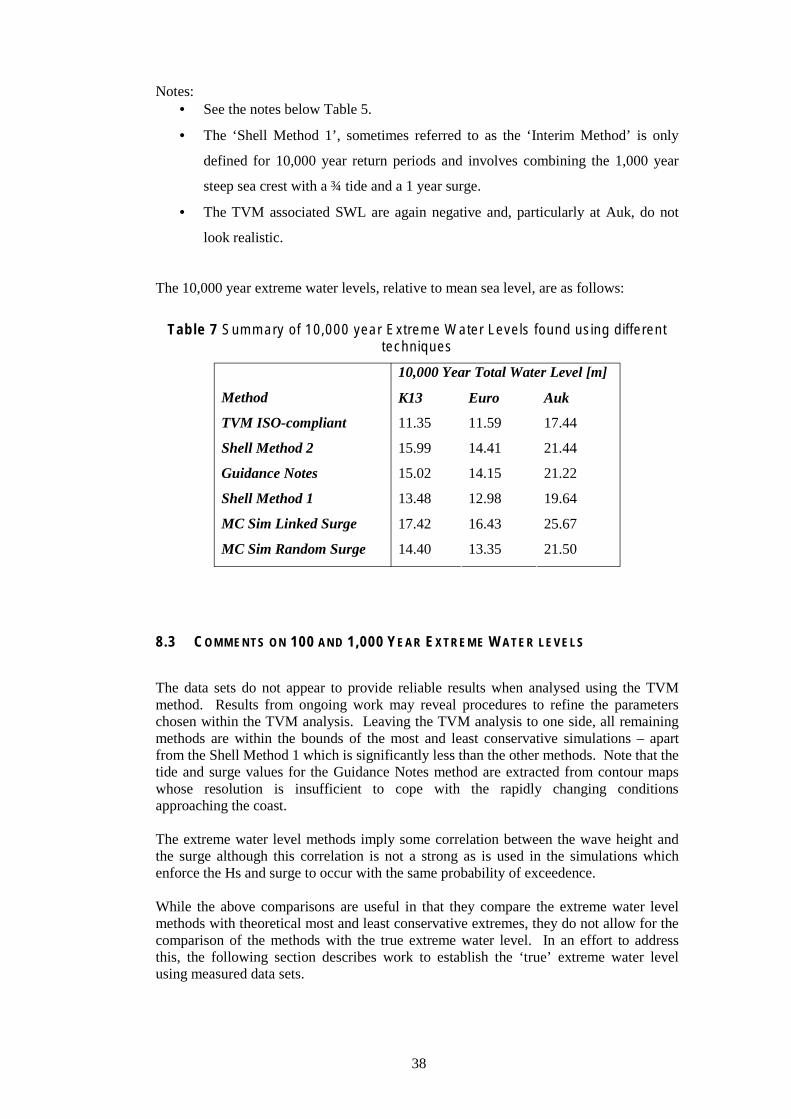
Notes: • See the notes below Table 5.

• The ‘Shell Method 1’, sometimes referred to as the ‘Interim Method’ is only

defined for 10,000 year return periods and involves combining the 1,000 year

steep sea crest with a ¾ tide and a 1 year surge.

• The TVM associated SWL are again negative and, particularly at Auk, do not

look realistic.

The 10,000 year extreme water levels, relative to mean sea level, are as follows:

Table 7 Summary of 10,000 year Extreme Water Levels found using different techniques

10,000 Year Total Water Level [m]

Method K13 Euro Auk

TVM ISO-compliant 11.35 11.59 17.44

Shell Method 2 15.99 14.41 21.44

Guidance Notes 15.02 14.15 21.22

Shell Method 1 13.48 12.98 19.64

MC Sim Linked Surge 17.42 16.43 25.67

MC Sim Random Surge 14.40 13.35 21.50

8.3 COMMENTS ON 100 AND 1,000 YEAR EXTREME WATER LEVELS

The data sets do not appear to provide reliable results when analysed using the TVM method. Results from ongoing work may reveal procedures to refine the parameters chosen within the TVM analysis. Leaving the TVM analysis to one side, all remaining methods are within the bounds of the most and least conservative simulations – apart from the Shell Method 1 which is significantly less than the other methods. Note that the tide and surge values for the Guidance Notes method are extracted from contour maps whose resolution is insufficient to cope with the rapidly changing conditions approaching the coast.

The extreme water level methods imply some correlation between the wave height and the surge although this correlation is not a strong as is used in the simulations which enforce the Hs and surge to occur with the same probability of exceedence.

While the above comparisons are useful in that they compare the extreme water level methods with theoretical most and least conservative extremes, they do not allow for the comparison of the methods with the true extreme water level. In an effort to address this, the following section describes work to establish the ‘true’ extreme water level using measured data sets.

38

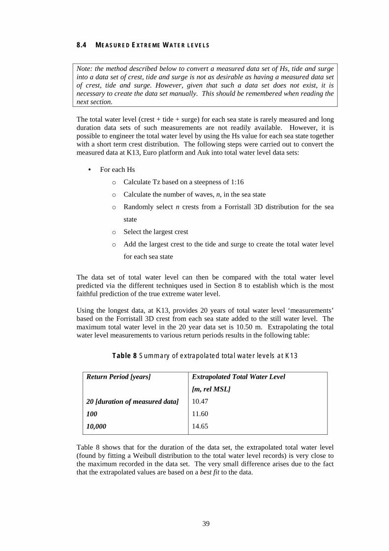
8.4 MEASURED EXTREME WATER LEVELS

Note: the method described below to convert a measured data set of Hs, tide and surge into a data set of crest, tide and surge is not as desirable as having a measured data set of crest, tide and surge. However, given that such a data set does not exist, it is necessary to create the data set manually. This should be remembered when reading the next section.

The total water level (crest + tide + surge) for each sea state is rarely measured and long duration data sets of such measurements are not readily available. However, it is possible to engineer the total water level by using the Hs value for each sea state together with a short term crest distribution. The following steps were carried out to convert the measured data at K13, Euro platform and Auk into total water level data sets:

• For each Hs

o Calculate Tz based on a steepness of 1:16

o Calculate the number of waves, n, in the sea state

o Randomly select n crests from a Forristall 3D distribution for the sea

state

o Select the largest crest

o Add the largest crest to the tide and surge to create the total water level

for each sea state

The data set of total water level can then be compared with the total water level predicted via the different techniques used in Section 8 to establish which is the most faithful prediction of the true extreme water level.

Using the longest data, at K13, provides 20 years of total water level ‘measurements’ based on the Forristall 3D crest from each sea state added to the still water level. The maximum total water level in the 20 year data set is 10.50 m. Extrapolating the total water level measurements to various return periods results in the following table:

Table 8 Summary of extrapolated total water levels at K13

Return Period [years] Extrapolated Total Water Level

[m, rel MSL]

20 [duration of measured data] 10.47

100 11.60

10,000 14.65

Table 8 shows that for the duration of the data set, the extrapolated total water level (found by fitting a Weibull distribution to the total water level records) is very close to the maximum recorded in the data set. The very small difference arises due to the fact that the extrapolated values are based on a best fit to the data.

39

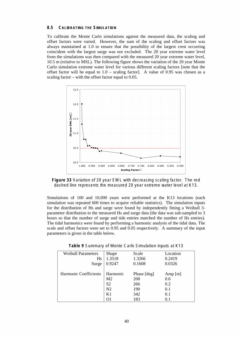
8.5 CALIBRATING THE SIMULATION

To calibrate the Monte Carlo simulations against the measured data, the scaling and offset factors were varied. However, the sum of the scaling and offset factors was always maintained at 1.0 to ensure that the possibility of the largest crest occurring coincident with the largest surge was not excluded. The 20 year extreme water level from the simulations was then compared with the measured 20 year extreme water level, 10.5 m (relative to MSL). The following figure shows the variation of the 20 year Monte Carlo simulation extreme water level for various different scaling factors [note that the offset factor will be equal to 1.0 – scaling factor]. A value of 0.95 was chosen as a scaling factor – with the offset factor equal to 0.05.

10.0

10.5

11.0

11.5

12.0

12.5

0.500 0.550 0.600 0.650 0.700 0.750 0.800 0.850 0.900 0.950 1.000

Scaling Factor

20yearEWL[m]

Figure 33 Variation of 20 year EWL with decreasing scaling factor. The red dashed line represents the measured 20 year extreme water level at K13.

Simulations of 100 and 10,000 years were performed at the K13 locations (each simulation was repeated 600 times to acquire reliable statistics). The simulation inputs for the distribution of Hs and surge were found by independently fitting a Weibull 3parameter distribution to the measured Hs and surge data (the data was sub-sampled to 3 hours so that the number of surge and tide entries matched the number of Hs entries). The tidal harmonics were found by performing a harmonic analysis of the tidal data. The scale and offset factors were set to 0.95 and 0.05 respectively. A summary of the input parameters is given in the table below.

Table 9 Summary of Monte Carlo Simulation inputs at K13

Weibull Parameters Shape Scale Location Hs 1.3518 1.3266 0.2419

Surge 0.9247 0.1608 0.0326

Harmonic Coefficients Harmonic Phase [deg] Amp [m] M2 208 0.6 S2 266 0.2 N2 190 0.1 K1 342 0.1 O1 183 0.1

40

8.6 100 AND 10,000 YEAR RETURN PERIOD EXTREME WATER LEVELS

The following table summarises the crest and SWL results at the 100 and 10,000 year return period.

Table 10 Comparison of 100 and 10,000 year return periods at K13

100year EWL 10,000 year EWL

Method

TVM ISO-compliant 9.39 11.35

Shell Method 2 12.34 15.99

Guidance Notes 11.79 15.02

Shell Method 1 --- 13.48

MC Sim Linked Surge 11.86 15.57

Extrapolation of measured data 11.60 14.65

ISO 19902 ‘Associated’ --- 17.17

ISO 19902 ‘Independent’ --- 14.87

Notes: • The ISO19902 ‘Independent’ case is defined as

h = √(a 2 + s 2 + t 2) + f

and the ISO19902 ‘Associated’ case is defined as

h = √((a + s) 2 + t 2) + f

where:

a is the abnormal wave crest height [10,000 year Crest]

s is the extreme storm surge [100 year Surge]

t is the maximum elevation of the tide relative to mean sea level [HAT]

f is the expected sum of subsidence, settlement and sea level rise over the design service life of the structure [set to zero in this example]

• The ISO19902 methods are only defined for the 10,000 year return period

Table 10 shows that for both the 100 and 10,000 year return periods, the extrapolated measured data is in good agreement with the Monte Carlo simulations although the Monte Carlo results are slightly higher than the extrapolated measured data results at both return periods. The TVM method predicts extreme values which are well outside range of all other techniques which leads to it being considered less applicable. Results from ongoing work may reveal procedures to refine the parameters chosen within the TVM analysis and enhance its applicability. At the 100 year return period, the results, excluding the TVM analysis, are within 75 cm of each other. At the 10,000 year return period, again excluding the TVM analysis, the results range from the Shell Method 1

41

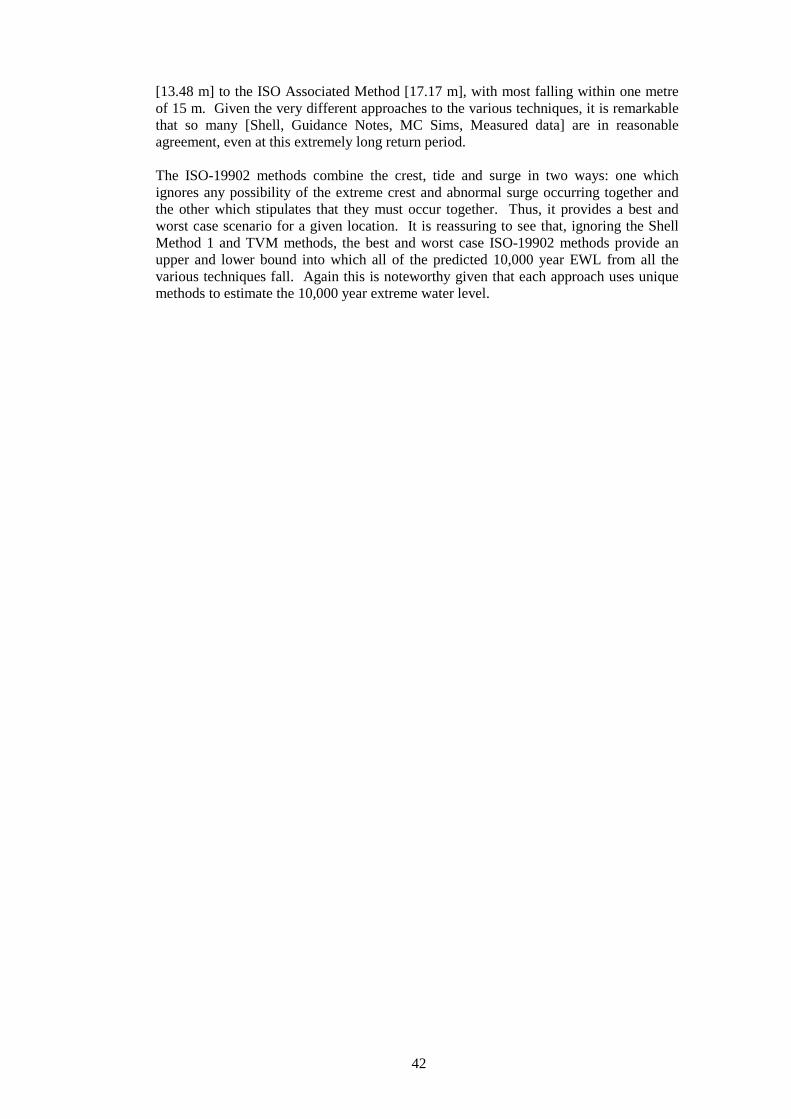
[13.48 m] to the ISO Associated Method [17.17 m], with most falling within one metre of 15 m. Given the very different approaches to the various techniques, it is remarkable that so many [Shell, Guidance Notes, MC Sims, Measured data] are in reasonable agreement, even at this extremely long return period.

The ISO-19902 methods combine the crest, tide and surge in two ways: one which ignores any possibility of the extreme crest and abnormal surge occurring together and the other which stipulates that they must occur together. Thus, it provides a best and worst case scenario for a given location. It is reassuring to see that, ignoring the Shell Method 1 and TVM methods, the best and worst case ISO-19902 methods provide an upper and lower bound into which all of the predicted 10,000 year EWL from all the various techniques fall. Again this is noteworthy given that each approach uses unique methods to estimate the 10,000 year extreme water level.

42

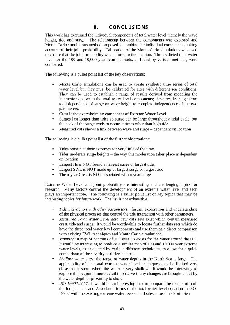
9. CONCLUSIONS This work has examined the individual components of total water level, namely the wave height, tide and surge. The relationship between the components was explored and Monte Carlo simulations method proposed to combine the individual components, taking account of their joint probability. Calibration of the Monte Carlo simulations was used to ensure that the joint probability was tailored to the location. The predicted total water level for the 100 and 10,000 year return periods, as found by various methods, were compared.

The following is a bullet point list of the key observations:

• Monte Carlo simulations can be used to create synthetic time series of total water level but they must be calibrated for sites with different sea conditions. They can be used to establish a range of results derived from modeling the interactions between the total water level components; these results range from total dependence of surge on wave height to complete independence of the two parameters.

• Crest is the overwhelming component of Extreme Water Level • Surges last longer than tides so surge can be large throughout a tidal cycle, but

the peak of the surge tends to occur at times other than high tide • Measured data shows a link between wave and surge – dependent on location

The following is a bullet point list of the further observations:

• Tides remain at their extremes for very little of the time • Tides moderate surge heights – the way this moderation takes place is dependent

on location • Largest Hs is NOT found at largest surge or largest tide. • Largest SWL is NOT made up of largest surge or largest tide • The n-year Crest is NOT associated with n-year surge

Extreme Water Level and joint probability are interesting and challenging topics for research. Many factors control the development of an extreme water level and each plays an important role. The following is a bullet point list of key topics that may be interesting topics for future work. The list is not exhaustive.

• Tide interaction with other parameters: further exploration and understanding of the physical processes that control the tide interaction with other parameters.

• Measured Total Water Level data: few data sets exist which contain measured crest, tide and surge. It would be worthwhile to locate further data sets which do have the three total water level components and use them as a direct comparison with existing EWL techniques and Monte Carlo simulations.

• Mapping: a map of contours of 100 year Hs exists for the water around the UK. It would be interesting to produce a similar map of 100 and 10,000 year extreme water levels, as calculated by various different techniques, to allow for a quick comparison of the severity of different sites.

• Shallow water sites: the range of water depths in the North Sea is large. The applicability of the usual extreme water level techniques may be limited very close to the shore where the water is very shallow. It would be interesting to explore this region in more detail to observe if any changes are brought about by the water depth or proximity to shore.

• ISO 19902:2007: it would be an interesting task to compare the results of both the Independent and Associated forms of the total water level equation in ISO19902 with the existing extreme water levels at all sites across the North Sea.

43

10. APPENDIX: SOFTWARE TESTING

10.1 SOFTWARE TESTING

First, simulations were run to ensure that the software was performing correctly. 100 years of data were simulated 1,000 times. A cutoff was employed and any sea states whose Hs values were below the cutoff were not processed. As the outputs from the simulation are the extreme values, the cutoff does not affect the results so long as the cutoff is not too high. For the central North Sea, a cutoff of 7 m was used in the 100 year simulations. Simulation inputs are detailed in the next section.

10.1.1 Input Data

The simulation was tested against a measured 25 year data set from the central North sea. The data set was chosen because it provided a source of data which is not otherwise used in this report – thus it provides ‘external’ verification of the simulation software. The data set comprises 25 years of measured significant wave height which was fitted using a 3 parameter Weibull distribution with the following parameters:

Shape: 1.1915 Scale: 1.5727 Location: 0.5741 100 year Hs: 13.14 m

The surge and tide distributions are again based on measured data from the central North Sea and are fitted as follows:

Normal Surge Weibull Surge: Maximum central value: 0.70 Shape: 1.543 Variance: 0.25 Scale: 0.214

Location -0.034 100 year surge: 1.03 m

Tide: Harmonic Amplitude [m] Phase [deg] M2 0.7 218 S2 0.2 357 N2 0.1 34 K1 0.1 197 O1 0.1 287

44

10.1.2 Hs

The results below show that the software is correctly predicting the 100 year Hs values and the distribution of Hs and crest heights is realistic. The simulated 100 year Hs value is 13.15 m.

0

1

0.1

0.2

0.3

0.4

0.5

0.6

0.7

0.8

0.9

Probability

Non

Exceedence

Simulated Hs

Theoretical [Weibull]

Simulated Crest

10 12 14 16 18 20 22

100 Year value [m]

Figure 34 Comparison between simulated and theoretical 100 year Hs values

10.1.3 Surges

The different options for including surges in the simulation were tested and the distribution of surges associated with the largest crest+surge for each sea state were plotted. The results are shown in the following figures and confirm that the surge distributions are being implemented correctly. Note that only statistics for Hs values above the cutoff are shown in the following plots and that the striped effect on the plots is simply due to the resolution of the images and is not a feature of the underlying data.

10.1.3.1 Random normal Surges

Figure 35 shows the results of using a surge which is normally distributed around a mean value which is chosen, at random, for each sea state. The maximum mean value is set at 0.7 m with the variance of the normal distribution set at 0.25.

45

24

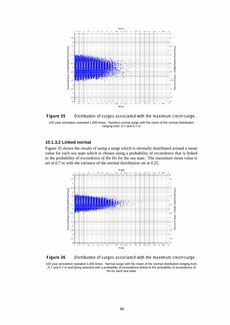
Figure 35 Distribution of surges associated with the maximum crest+surge. 100 year simulation repeated 1,000 times. Random normal surge with the mean of the normal distribution

ranging from -0.7 and 0.7 m

10.1.3.2 Linked normal Figure 35 shows the results of using a surge which is normally distributed around a mean value for each sea state which is chosen using a probability of exceedence that is linked to the probability of exceedence of the Hs for the sea state. The maximum mean value is set at 0.7 m with the variance of the normal distribution set at 0.25.

Figure 36 Distribution of surges associated with the maximum crest+surge. 100 year simulation repeated 1,000 times. Normal surge with the mean of the normal distribution ranging from -0.7 and 0.7 m and being selected with a probability of exceedence linked to the probability of exceedence of

Hs for each sea state

46

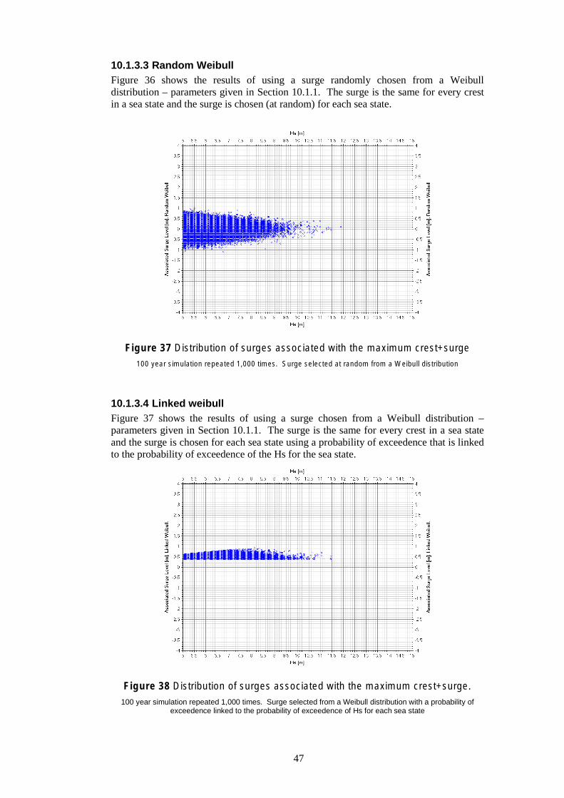
10.1.3.3 Random Weibull Figure 36 shows the results of using a surge randomly chosen from a Weibull distribution – parameters given in Section 10.1.1. The surge is the same for every crest in a sea state and the surge is chosen (at random) for each sea state.

Figure 37 Distribution of surges associated with the maximum crest+surge 100 year simulation repeated 1,000 times. Surge selected at random from a Weibull distribution

10.1.3.4 Linked weibull Figure 37 shows the results of using a surge chosen from a Weibull distribution – parameters given in Section 10.1.1. The surge is the same for every crest in a sea state and the surge is chosen for each sea state using a probability of exceedence that is linked to the probability of exceedence of the Hs for the sea state.

Figure 38 Distribution of surges associated with the maximum crest+surge. 100 year simulation repeated 1,000 times. Surge selected from a Weibull distribution with a probability of

exceedence linked to the probability of exceedence of Hs for each sea state

47

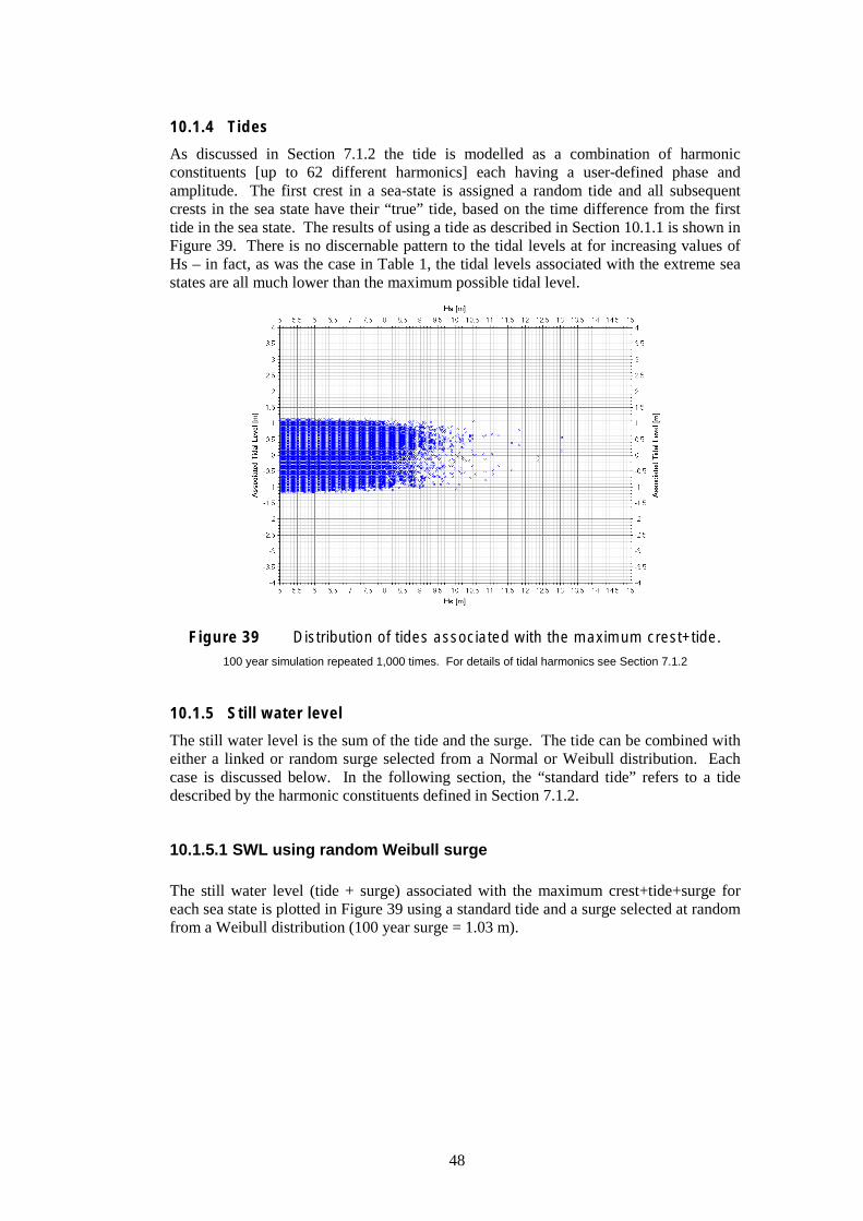
10.1.4 Tides

As discussed in Section 7.1.2 the tide is modelled as a combination of harmonic constituents [up to 62 different harmonics] each having a user-defined phase and amplitude. The first crest in a sea-state is assigned a random tide and all subsequent crests in the sea state have their “true” tide, based on the time difference from the first tide in the sea state. The results of using a tide as described in Section 10.1.1 is shown in Figure 39. There is no discernable pattern to the tidal levels at for increasing values of Hs – in fact, as was the case in Table 1, the tidal levels associated with the extreme sea states are all much lower than the maximum possible tidal level.

Figure 39 Distribution of tides associated with the maximum crest+tide. 100 year simulation repeated 1,000 times. For details of tidal harmonics see Section 7.1.2

10.1.5 Still water level

The still water level is the sum of the tide and the surge. The tide can be combined with either a linked or random surge selected from a Normal or Weibull distribution. Each case is discussed below. In the following section, the “standard tide” refers to a tide described by the harmonic constituents defined in Section 7.1.2.

10.1.5.1 SWL using random Weibull surge

The still water level (tide + surge) associated with the maximum crest+tide+surge for each sea state is plotted in Figure 39 using a standard tide and a surge selected at random from a Weibull distribution (100 year surge = 1.03 m).

48

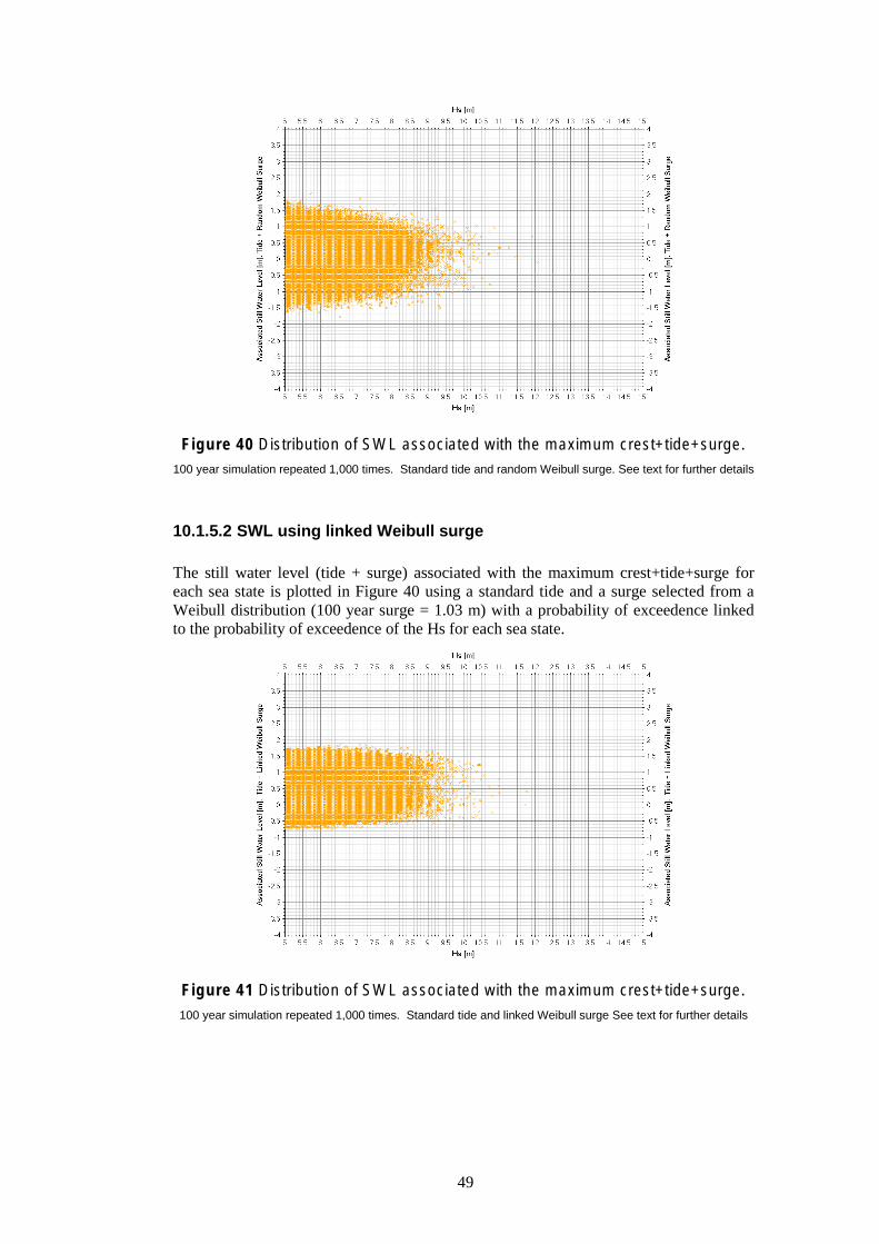
Figure 40 Distribution of SWL associated with the maximum crest+tide+surge. 100 year simulation repeated 1,000 times. Standard tide and random Weibull surge. See text for further details

10.1.5.2 SWL using linked Weibull surge

The still water level (tide + surge) associated with the maximum crest+tide+surge for each sea state is plotted in Figure 40 using a standard tide and a surge selected from a Weibull distribution (100 year surge = 1.03 m) with a probability of exceedence linked to the probability of exceedence of the Hs for each sea state.

Figure 41 Distribution of SWL associated with the maximum crest+tide+surge.

100 year simulation repeated 1,000 times. Standard tide and linked Weibull surge See text for further details

49

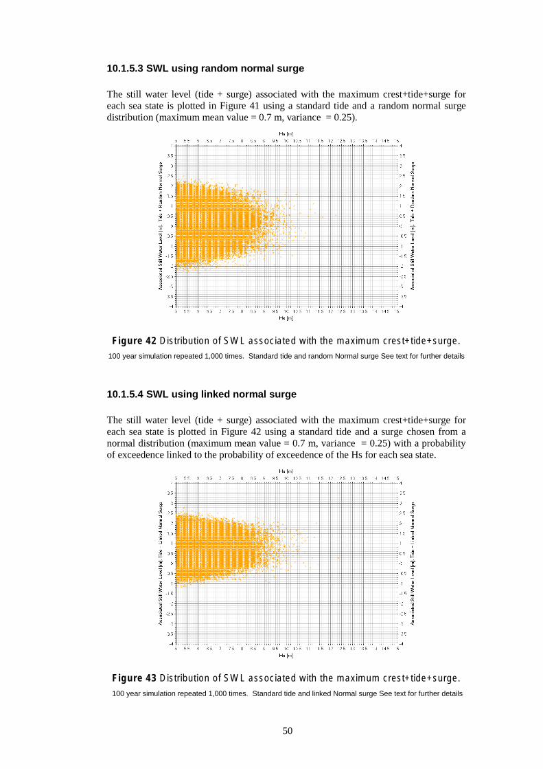
10.1.5.3 SWL using random normal surge

The still water level (tide + surge) associated with the maximum crest+tide+surge for each sea state is plotted in Figure 41 using a standard tide and a random normal surge distribution (maximum mean value = 0.7 m, variance = 0.25).

Figure 42 Distribution of SWL associated with the maximum crest+tide+surge. 100 year simulation repeated 1,000 times. Standard tide and random Normal surge See text for further details

10.1.5.4 SWL using linked normal surge

The still water level (tide + surge) associated with the maximum crest+tide+surge for each sea state is plotted in Figure 42 using a standard tide and a surge chosen from a normal distribution (maximum mean value = 0.7 m, variance = 0.25) with a probability of exceedence linked to the probability of exceedence of the Hs for each sea state.

Figure 43 Distribution of SWL associated with the maximum crest+tide+surge.

100 year simulation repeated 1,000 times. Standard tide and linked Normal surge See text for further details

50

10.1.6 Summary

Max crest + “anything” is dominated by the crest – which often occurs in a sea state OTHER than the one with the largest Hs. The associated “anything” is less than its largest possible value for the extreme crest + “anything”. Even when the surge is forced to occur with a similar probability of exceedence as the Hs for a given sea state, the SWL associated with the extreme crest+tide+surge is much smaller than its largest possible value.

51

Published by the Health and Safety Executive 10/09


A Monte Carlo approach to joint probability of wave, tide and surge in extreme water level calculations Extreme Water Level is the total level of the water arising from wave crest, storm surge and tidal level acting in combination with each other throughout an extreme event. Individually, each of these components is relatively well understood. However, the combination of these components is not straightforward and depends on the conditions of the location in question. This study addresses the behaviour of the individual components, their interaction, and their joint probability, leading to the development of a Monte Carlo based approach to the estimation of Extreme Water Level. The study concludes with a review of latest ISO guidance on estimating extreme water levels and a comparison between extreme water level results derived using existing methods, ISO guidance and Monte Carlo simulations.

This report and the work it describes were funded by the Health and Safety Executive (HSE). Its contents, including any opinions and/or conclusions expressed, are those of the author alone and do not necessarily reflect HSE policy.

RR740

www.hse.gov.uk

a monte carlo approach to joint probability of wave, tide … · · 2017-07-15executive health...

Documents