a model-based robust control approach for bilateral ... · a model-based robust control approach...
TRANSCRIPT

A model-based robust control approach for bilateralteleoperation systemsLopez Martinez, C.A.
DOI:10.6100/IR784500
Published: 01/01/2015
Document VersionPublisher’s PDF, also known as Version of Record (includes final page, issue and volume numbers)
Please check the document version of this publication:
• A submitted manuscript is the author's version of the article upon submission and before peer-review. There can be important differencesbetween the submitted version and the official published version of record. People interested in the research are advised to contact theauthor for the final version of the publication, or visit the DOI to the publisher's website.• The final author version and the galley proof are versions of the publication after peer review.• The final published version features the final layout of the paper including the volume, issue and page numbers.
Link to publication
Citation for published version (APA):Lopez Martinez, C. A. (2015). A model-based robust control approach for bilateral teleoperation systemsEindhoven: Technische Universiteit Eindhoven DOI: 10.6100/IR784500
General rightsCopyright and moral rights for the publications made accessible in the public portal are retained by the authors and/or other copyright ownersand it is a condition of accessing publications that users recognise and abide by the legal requirements associated with these rights.
• Users may download and print one copy of any publication from the public portal for the purpose of private study or research. • You may not further distribute the material or use it for any profit-making activity or commercial gain • You may freely distribute the URL identifying the publication in the public portal ?
Take down policyIf you believe that this document breaches copyright please contact us providing details, and we will remove access to the work immediatelyand investigate your claim.
Download date: 28. Jun. 2018

A Model-based Robust Control Approach
for Bilateral Teleoperation Systems
Cesar Augusto Lopez Martınez

The research reported in this thesis is part of the research program of the DutchInstitute of Systems and Control (DISC). The author has successfully completedthe educational program of the Graduate School DISC.
This research was supported partially by the Percutaneous Instruments TeleOper-ated Needles (PITON) project funded by Agentschap NL, an agency of the DutchMinistry of Economy Affairs.
A catalogue record is available from the Eindhoven University of TechnologyLibrary. ISBN: 978-90-386-3768-6
Typeset by the author with the pdfLATEX documentation system.Cover design: Cesar A. Lopez M. and Nina Simons. Background based on imageunder creative commons license. Pictures by Thijs Meenink.Reproduction: Ipskamp Drukkers B.V., Enschede, The Netherlands.
Copyright 2015 by Cesar Augusto Lopez Martınez. All rights reserved.

A Model-based Robust Control Approach
for Bilateral Teleoperation Systems
PROEFSCHRIFT
ter verkrijging van de graad van doctor aan deTechnische Universiteit Eindhoven, op gezag van de
rector magnificus, prof.dr.ir. C.J. van Duijn, voor eencommissie aangewezen door het College voor
Promoties, in het openbaar te verdedigenop dinsdag 10 februari 2015 om 16.00 uur
door
Cesar Augusto Lopez Martınez
geboren te Aguachica, Colombia

Dit proefschrift is goedgekeurd door de promotoren en de samenstelling van depromotiecommissie is als volgt:
voorzitter: prof.dr. L.P.H. de Goey1e promotor: prof.dr.ir. M. Steinbuch2e promotor: prof.dr. S. Weilandcopromotor: dr.ir. M.J.G. van Molengraftleden: prof.dr. H. Nijmeijer
prof.dr.ir. Stefano Stramigioli (Universiteit Twente)dr. D. Constantinescu (University of Victoria)
adviseur: dr. E. Vander Poorten (Katholieke Universiteit Leuven)

i
Societal Summary
Bilateral teleoperation systems allow to manipulate and sense a remote or difficultto access environment. Imagine a system that allows a surgeon to command roboticinstruments inside your body with high precision, and moreover, that provides thesurgeon the feeling of how rigid the surrounding tissue is. This latter characteristic,called force feedback, can help the surgeon not to exert excessive force on delicatetissues, preventing damage. This means that the patients will have less traumaand faster recovery times after surgery, which will also reduce the costs of thehealthcare system.
Robotic surgery is already a reality, however, state of the art systems do not pro-vide high quality force feedback to the operator. This is because high quality forcefeedback always includes a compromise in the stability of the system, and cur-rent techniques do not provide a good balance. Control of bilateral teleoperationsystems is not a trivial task, on one hand because the operating environment canvary largely and on the other hand because the system directly interacts with thehuman being. Therefore, the force feedback to the operator needs to be designedin a clever way.
In this PhD thesis I propose a methodology to design and safely implement highquality force feedback in bilateral teleoperation systems. The method involvesmodelling of the human operator and the use of specific environment models. Thisresearch represents a step towards bringing force feedback capabilities in roboticsurgery systems, which will have a direct impact in the human healthcare system.

ii
iii
SummaryA Model-based Robust Control Approach for Bilateral Teleoperation Systems
Bilateral teleoperation systems allow an operator to manipulate a remote environ-ment by means of a master and a slave device while using force feedback to obtaina feeling of tele-presence. The system is supposed to deliver high performancein that the operator feels as if he/she is manipulating the environment directly,in a stable fashion. However, there is an inherent trade-off between stability andperformance, and it is a challenging problem to design controllers that meet anappropriate balance. Most of the current design tools are based on passivity the-ory, which guarantees stability but does not provide means to achieve a systematicstability/performance trade-off. Moreover, the dynamics of both environment andoperator are inherently time-varying, which aspect is often overlooked. Luckily,in many applications such as minimally invasive surgery (MIS), needle insertion,suturing, etc., the environment properties vary in a bounded set, e.g. the stiffnessof tissue inside a patient under surgery. Therefore, the work in this thesis exploitsthe knowledge on the bounds of variation in both environment and operator forthe purpose of control design.
This thesis adopts a model-based robust control design approach. As a firststep, we model the teleoperation system, including an appropriate description ofits uncertain dynamics. We consider environments in which the stiffness is thedominant phenomenon, e.g. in stiffness palpation tasks present in surgery. For thehuman operator, we have constructed a parametric model based on identificationexperiments, in which the operator stiffness appeared as the dominant varyingparameter. Both the environment stiffness and the operator stiffness are treatedas parametric uncertainties, which are considered to be bounded and time-varyingto account for realistic behaviour. Subsequently, controller synthesis is done viarobust control techniques based on Linear Matrix Inequalities (LMI). The opera-tor/environment uncertainty is described via a specific class of Integral QuadraticConstraints (IQCs), which allow to represent the parametric uncertainties as ar-

iv
bitrarily fast time-varying.
Based on the above approach, we propose and validate different controller de-signs. In our first design a single controller for the considered range of stiffnessvariation is designed, for which simulations and experiments are performed with aone degree-of-freedom (1-DoF) academic bilateral teleoperation setup. The resultsshow that the closed loop system presents robust performance for the bounded setof uncertainty for which it was designed, including sudden changes in the envi-ronment stiffness. The result from experiments matches the theoretical stabilityresult, which validates the assumptions made during modelling and control syn-thesis. Next, we consider an extended the range of stiffness variation to accountfor hard contacts, e.g. in contact with bones present in surgery. In such case, onecontroller might not be sufficient to achieve a desired performance. Therefore, ina second design, to improve performance we propose a multi-controller structure,in which we design multiple robust controllers for different regions of environmentstiffness, which controllers are scheduled on the basis of an estimate of the envi-ronment stiffness. Moreover, all the controllers are designed to share a commonlyapunov function to guarantee smooth switching between them. This approach issimulated and experimentally validated in the 1-DoF setup. The results show thata multi-controller structure can provide an improved performance for the same setof uncertainties, compared with a single controller structure. In a third design,the requirement of a common lyapunov function in the multi-controller structure isrelaxed via dwell time conditions during the controller synthesis for the purpose ofobtaining an improved performance, which is validated in simulations of an 1-DoFsetup. In a fourth design, we relax completely the requirement of a common lya-punov function in the multi-controller structure, designing multiple performance-optimized controllers independently and switching between them using an adaptedversion of the bumpless transfer technique. Simulations and experiments in the1-DoF setup validate the designed multicontroller controller architecture. Finally,the proposed model-based robust control methodology is implemented on a real-lifesurgical robot named Sofie, which has non-ideal properties compared to academicsetups, for instance the slave device is non-backdrivable, it is heavy and has highlevels of friction, moreover, the master device has structural resonances and doesnot have force sensor. The experimental results show that the proposed methodscan be also successfully applied to such type of teleoperators.
v
Contents
Societal Summary i
Summary iii
1 Introduction 11.1 Bilateral teleoperation . . . . . . . . . . . . . . . . . . . . . . . . . 1
1.1.1 Teleoperation systems and force feedback . . . . . . . . . . 11.1.2 A definition of stability for bilateral teleoperation systems . 41.1.3 Bilateral control design . . . . . . . . . . . . . . . . . . . . 71.1.4 Pros and cons of current bilateral control design methods . 9
1.2 Problem statement and challenges . . . . . . . . . . . . . . . . . . 131.3 Research approach . . . . . . . . . . . . . . . . . . . . . . . . . . . 141.4 Contributions . . . . . . . . . . . . . . . . . . . . . . . . . . . . . . 221.5 Outline of the thesis . . . . . . . . . . . . . . . . . . . . . . . . . . 23
2 Robust Bilateral Control under Time-Varying Dynamics 272.1 Introduction . . . . . . . . . . . . . . . . . . . . . . . . . . . . . . . 272.2 Model based robust control . . . . . . . . . . . . . . . . . . . . . . 30
2.2.1 LFR model of a teleoperation system . . . . . . . . . . . . . 302.2.2 Robust control design with guaranteed performance specifi-
cations . . . . . . . . . . . . . . . . . . . . . . . . . . . . . . 392.2.3 Weighting filter design . . . . . . . . . . . . . . . . . . . . . 46
2.3 Robust control applied to a 1-DoF academic setup . . . . . . . . . 482.3.1 Synthesis results . . . . . . . . . . . . . . . . . . . . . . . . 492.3.2 Simulation results . . . . . . . . . . . . . . . . . . . . . . . 542.3.3 Experiments . . . . . . . . . . . . . . . . . . . . . . . . . . 56
2.4 Conclusions . . . . . . . . . . . . . . . . . . . . . . . . . . . . . . . 61
3 Switching Robust Control for Bilateral Teleoperation 633.1 Introduction . . . . . . . . . . . . . . . . . . . . . . . . . . . . . . . 63

vi
3.2 Switching robust control approach . . . . . . . . . . . . . . . . . . 65
3.2.1 LFR model of a teleoperation system . . . . . . . . . . . . . 653.2.2 Switching robust control design using a common
quadratic Lyapunov function . . . . . . . . . . . . . . . . . 723.2.3 Tailor-made solution for bilateral teleoperation . . . . . . . 793.2.4 Environment estimation . . . . . . . . . . . . . . . . . . . . 823.2.5 Weighting filter design . . . . . . . . . . . . . . . . . . . . . 84
3.3 Switching robust control applied to a 1-DoF academic setup . . . . 853.3.1 Synthesis results . . . . . . . . . . . . . . . . . . . . . . . . 873.3.2 Simulation results . . . . . . . . . . . . . . . . . . . . . . . 883.3.3 Experiments . . . . . . . . . . . . . . . . . . . . . . . . . . 93
3.4 Conclusions . . . . . . . . . . . . . . . . . . . . . . . . . . . . . . . 99
4 Switching Robust Control via Dwell Time Conditions 1014.1 Introduction . . . . . . . . . . . . . . . . . . . . . . . . . . . . . . . 1014.2 Adding control design flexibility via dwell time conditions . . . . . 103
4.2.1 Model of the teleoperation system for switching robust control1034.2.2 Switching robust control design using multiple quadratic
Lyapunov functions . . . . . . . . . . . . . . . . . . . . . . 1074.3 Simulation results . . . . . . . . . . . . . . . . . . . . . . . . . . . 1154.4 Conclusions . . . . . . . . . . . . . . . . . . . . . . . . . . . . . . . 118
5 Bumpless Transfer of Robust Controllers for Teleoperation 1195.1 Introduction . . . . . . . . . . . . . . . . . . . . . . . . . . . . . . . 1195.2 Bumpless transfer in bilateral teleoperation . . . . . . . . . . . . . 121
5.2.1 Linear fractional representation of a teleoperation system . 1215.2.2 Uncertainty region distribution and robust control design . 1235.2.3 Bumpless transfer between robust controllers . . . . . . . . 1255.2.4 Environment estimation . . . . . . . . . . . . . . . . . . . . 126
5.3 Experimental results on a 1-DoF academic setup . . . . . . . . . . 1285.4 Conclusions . . . . . . . . . . . . . . . . . . . . . . . . . . . . . . . 132
6 Model-Based Robust Control for a Non-Ideal Teleoperator 1336.1 Introduction . . . . . . . . . . . . . . . . . . . . . . . . . . . . . . . 1336.2 Model based robust control applied to SOFIE robot . . . . . . . . 135
6.2.1 Experimental setup . . . . . . . . . . . . . . . . . . . . . . . 1356.2.2 Modelling of the teleoperation surgical system for control
synthesis . . . . . . . . . . . . . . . . . . . . . . . . . . . . 1396.2.3 Robust control under time-varying uncertainties . . . . . . 1466.2.4 Switching robust control via bumpless transfer of robust con-
trollers . . . . . . . . . . . . . . . . . . . . . . . . . . . . . . 1476.2.5 Environment estimation . . . . . . . . . . . . . . . . . . . . 149
6.3 Results of robust control applied on SOFIE robot . . . . . . . . . . 150

vii
6.3.1 Controller synthesis results . . . . . . . . . . . . . . . . . . 1516.3.2 Simulation results . . . . . . . . . . . . . . . . . . . . . . . 1546.3.3 Experiments . . . . . . . . . . . . . . . . . . . . . . . . . . 1566.3.4 Discussion . . . . . . . . . . . . . . . . . . . . . . . . . . . . 160
6.4 Conclusions . . . . . . . . . . . . . . . . . . . . . . . . . . . . . . . 161
7 Conclusions and Recommendations 1637.1 Conclusions . . . . . . . . . . . . . . . . . . . . . . . . . . . . . . . 1637.2 Recommendations for future research . . . . . . . . . . . . . . . . . 168
References 171
A 1-DoF Academic Setup 179
B Controller-Multiplier Synthesis Procedure 181B.1 Definitions of variables and set of LMIs . . . . . . . . . . . . . . . 181
B.1.1 Definitions common to all control synthesis methods . . . . 182B.1.2 Definitions for the synthesis method using a common Lya-
punov function and for the bumpless transfer method . . . 183B.1.3 Definitions for the synthesis method using dwell time condi-
tions . . . . . . . . . . . . . . . . . . . . . . . . . . . . . . . 185B.2 Synthesis procedure: version I . . . . . . . . . . . . . . . . . . . . . 188B.3 Synthesis procedure: version II . . . . . . . . . . . . . . . . . . . . 190
Acknowledgments / Dankwoord / Agradecimientos 193
Curriculum Vitae 197

viii

1
Chapter 1
Introduction
IN this chapter we introduce bilateral teleoperation systems. An overviewof the current literature on control design for teleoperation systems is
given in order to point out the unsolved challenges. Finally, the proposedmethods and the contributions of this thesis are discussed.
1.1 Bilateral teleoperation
1.1.1 Teleoperation systems and force feedback
The word teleoperation means “operation at a distance”, thus, a teleoperation sys-tem allows the human to interact with environments that for instance: are locatedremotely, or environments are not of easy access, or that can be hazardous for thehuman health. Examples of applications are illustrated in Fig. 1.1. For instance,a mobile robot can be driven from a distance to explore disaster areas. In thisscenario the robot might be equipped with special sensors to detect movementand heat to spot potential victims. Another application is a nuclear fusion reac-tor in which the level of radioactivity is dangerous for the operators. Thereforeit is desirable to do the maintenance of the reactor using a robotic arm which isplaced inside the reactor. The operator will be in another room sending commandsthrough a mechanical device and inspecting the process via cameras. Force feed-back can be provided to the operator, which can help him to move objects faster.In other types of applications, such as in robotically assisted minimally invasivesurgery, a robotic arm or needle can be inserted in the human body through smallincisions to reach internal organs. The surgeon can be situated right next to the

2 Chapter 1 Introduction
Figure 1.1: Different applications of teleoperation systems. From top-left tobottom-right: Maintenance in the Joint European Torus (JET) nuclear fusionreactor (picture by EFDA, visit www.efda.org); exploration of disaster areas usingthe RoboCup Rescue robot Hector from Darmstadt at 2010 German Open (pic-ture by Mike1024/Wikimedia Commons); robotic assisted surgery with the SOFIErobot by van den Bedem et al. (2010)(picture by Bart van Overbeeke/Bart vanOverbeeke Fotografie); robotic assisted eye surgery (Courtesy of PRECEYES ©).
patient interacting with a master device to drive the movements of the surgicalinstrument. It is desirable that, via the master device, the teleoperation systemprovides to the operator the kinaesthetic feeling of a stiffness similar to that ofthe environment, helping the surgeon to differentiate different types of tissues bymeans of palpation.
The mentioned applications have one thing in common: the fact that the oper-ator is sending commands that are executed by a robotic device, for instance toperform a specific movement. However, only in some of the mentioned applica-tions, force-feedback is provided from the environment to the operator. When suchforce feedback is present, the system is said to be bilaterally teleoperated. The typeof force feedback provided to the operator can vary significantly from one applica-tion to the other. For instance, in the reactor maintenance case, the environmentconsists mainly of rigid objects which have to be moved to a desired position. Onecan provide haptic information to the operator about when there is contact withan object. This might already help him/her to improve the task performance.On the other hand, in the robotic surgery application, it would be desirable forthe surgeon to distinguish the different types of tissues, such that he/she can feelthrough the master device a similar stiffness as that of the environment.

1.1 Bilateral teleoperation 3
Figure 1.2: Early bilateral teleoperators: first mechanical master-slave manipula-tors designed by John Payne (left) and Goertz (center), first electric master-slavemanipulator designed by Goertz and Thomposon (right). Images are taken fromCyberneticzoo (2010)
Force-feedback can improve the task performance significantly, however, whenforces are reflected to the operator they cause a reaction on his/her movements.These are passed again to the slave device, which again might result in a differ-ent force reflected to the operator. Such loops may cause instability during taskexecution, and it is more likely to happen if communication delays between themaster and the slave sides are present. Hence, determining what kind of feedbackis needed for a certain application or task is not a trivial problem, let alone itssafe implementation. In fact, during the last six decades, researchers have beenworking in studying bilateral teleoperation systems. Specifically on the interac-tions between the operator and the environment, and how to couple them in anefficient way by means of a master-slave system.
The first bilateral teleoperation systems appeared in the late 1940s and the early1950s. They were used mainly for the remote handling of hazardous materials. Ex-ample of these teleoperators are the systems designed by Payne (1949)(Patent filedin 1948) and by Goertz (1953)(Patent filed in 1949), see Fig. 1.2. In these devicesthe master and slave were mechanically coupled. Later, the first electrically con-trolled teleoperator was presented in Goertz and Thompson (1954), see Fig. 1.2.After that and until the late 1980s, there was an increased interest in telemanipula-tion, which encompassed with the increasing computational power and popularityof virtual reality. In that period researchers also started studying the effects ofdelays in teleoperation systems, and developed the initial control strategies for bi-lateral teleoperation based on supervisory control. It was then until the mid 1980s,when control theory started to develop, that more systematic approaches towardsanalysis and control design started to appear. Especially network theory came intoplay in teleoperation (see, e.g., Raju et al. (1989)), opening the path to techniqueslike passivity, scattering theory and wave variables, see, e.g., Niemeyer and Slotine(1991); Anderson and Spong (1989). Those theories were in particular motivated

4 Chapter 1 Introduction
to find solutions due to instability caused by delays in bilateral teleoperation sys-tems. Since then, variations of those theories have been and are still applied inanalysis and control design. Also, in the last two decades, techniques based onrobust control and H∞ have been applied widely to the teleoperation problem.Since then only few deep changes on the control methodologies have been pro-posed but rather variations on them, with the exception of some techniques suchas model mediated control, in which a model of the environment is obtained onlineand reflected to the operator (see, e.g., Mitra and Niemeyer (2008)), and sharedcontrol, in which the force feedback design is centered around the task itself (see,e.g., Abbink et al. (2012)). The reader is referred to the surveys in Hokayem andSpong (2006); Passenberg et al. (2010) for a more detailed overview on the differentdevelopments in the history of bilateral teleoperation.
After this brief overview of bilateral teleoperation systems, in the next sectionwe will focus on the most relevant developments on modelling and control designconcerning the research presented in this thesis.
1.1.2 A definition of stability for bilateral teleoperation systems
Before addressing the control design problem, we would like to discuss in moredepth what stability means for teleoperation systems. To illustrate the conceptof stability that is proposed here, consider a very simple teleoperation system: aperson cutting a piece from a cake with a knife, as illustrated in the right part ofFig. 1.3. In this case, the knife is considered as the teleoperator, i.e. the instrumentor tool that serves as a link between the operator and the environment. Moreover,the hand represents the operator and the cake represents the environment. Thehuman hand, the environment, the knife, the interaction between the hand and
Figure 1.3: A simple teleoperation system: a person that cuts a piece of cake.The hand represents the operator, the knife the teleoperator, and the cake theenvironment.
1.1 Bilateral teleoperation 5
the knife and the interaction between the knife and the cake constitute a bilateralteleoperation system.
Firstly, consider the knife, i.e. the teleoperator, as shown in the left part of Fig. 1.3.This system is fully defined in the sense that its motion dynamics can be repre-sented by
x = f(x, t), (1.1)
in which x represents the state of the motion dynamics of the knife, f(x, t) is apossibly nonlinear function and t is the time variable. Intuitively, one can say thata knife lying on a table (not shown in Fig. 1.3) is a “stable” system. More formally,the motion dynamics of the knife define an asymptotically stable system in thesense that small perturbations result in movements that will vanish over time anda new equilibrium is reached. At this point we have to consider the interactionbetween the knife and the table due to gravity as part of the teleoperator aswell. For instance, the friction between the table and the knife makes the knifemovements to reach equilibrium.
Next, consider the case when the knife is dropped and it buries into the cake. Thissituation is shown in the center part of Fig. 1.3. There is a difference with theprevious case: the resulting system is not fully defined, i.e. it cannot be representedwith dynamics of the form in Eq. (1.1) . This because we do not know exactlythe consistency of the cake, i.e. its dynamics. However, one can use a systemwith uncertainty ∆e to describe the set of dynamics of different cakes. Therefore,the knife-cake system can be considered as an uncertain system, the dynamics ofwhich can be described by the following system
x = g(x,∆e, t),
in which x now also includes the state of the motion dynamics of the cake andg(x,∆e, t) is a possibly nonlinear function. Again, one can say intuitively thatthe knife-cake system is “stable” in the sense that the knife will be at rest at acertain location in the cake. In a more formal framework, the stability of theknife-cake system has the following meaning: the knife can enter the cake (whichhas uncertain dynamics) in different ways (that is, different initial conditions), andthe knife’s movement will end up in an equilibrium point depending on the cake’sconsistency, described by the uncertainty ∆e. If for all predefined consistencylevels ∆e ∈ ∆e the knife reaches an equilibrium point, we call the knife-cakesystem robustly stable with respect to the uncertainty level ∆e.
Finally, consider the situation in which a person grabs the knife and cuts the cakeas shown in the right part of Fig. 1.3. Additional to the uncertainty ∆e of thecake, the hand also exhibits uncertain dynamics. For instance, the operator cangrab the knife with a light or a tight grip. In both of these cases the hand will

6 Chapter 1 Introduction
have different dynamics. Thus, the hand behavior while interacting with the knifecould be described with a system with dynamic uncertainty ∆h. Moreover, thehand exerts an input u to the system. This input allows to command the knife’smovements. Such type of system could be described by the following equation
x = h(x, u,∆h,∆e, t), (1.2)
which is an “open” system because of the presence of the “free will” of the humanto exert a certain force with his/her hand. h(x, u,∆h,∆e, t) is a possibly nonlinearfunction.Once again, one can assume that the hand-knife-cake system is “stable”in the sense that we can perform the desired task of cutting a piece from thecake in a safe way. More formally, there is a main difference with the other twocases: during the execution of the task, there will not always be an equilibriumpoint of the knife’s movements. Rather, we can say that the movements of theknife remain bounded, provided that the input u exerted by the hand remainsalso bounded, under the presence of the uncertainties ∆h and ∆e. Thus, it is saidthat this system presents robust bounded input to bounded state stability. Thisconcept is also known as Input to State Stability (ISS) and it is illustrated in detailin the work of Sontag (2008). Precisely, the ISS concept of robust stability willbe adopted for bilateral teleoperation systems in the rest of this thesis, and it ishereafter simply referred to as the stability of the bilateral teleoperation system.
Up to this point, it is assumed that the system with uncertainty in Eq. (1.2)covers exactly the uncertain dynamics of the true bilateral teleoperation system.In practice, the mathematical function h(x, u,∆h,∆e, t) and the uncertainties ∆h
and ∆e are approximate models. Thus, hereafter we assume that Eq. (1.2) and itscomponents represent a model, which not necessarily covers exactly the uncertaindynamics of the real system. Hence, the stability analysis of a bilateral teleoper-ation system depends on the type of uncertainties ∆h ∈ ∆h and ∆e ∈ ∆e thatare used in the model. Moreover, those uncertainties can be defined to describespecific dynamics present in a certain application of the bilateral teleoperationsystem.
We also illustrate the concept of conservatism in the stability analysis of bilateralteleoperation systems. Define two pairs of set of uncertainties of the operator andthe environment dynamics: (∆
′
h,∆′
e) and (∆′′
h,∆′′
e ). Hence, if ∆′′
h ⊂∆′
h and/or
∆′′
e ⊂ ∆′
e, then achieving robust stability of the system in Eq. (1.2) could beeasier for the pair (∆
′′
h,∆′′
e ) than for the pair (∆′
h,∆′
e). Therefore, the latter setis said to introduce conservatism in the robust stability test, assuming that boththe considered sets cover at least the set of uncertainties present in the real systemfor a specific application.
To illustrate this concept, imagine that we replace the common knife by an electricknife. Most probably, one cannot say that the electric knife itself is “stable” when it

1.1 Bilateral teleoperation 7
is ‘on’ and it has no human control. For instance, throwing the electrical knife intothe cake will have very undesired results in the sense that the vibrations could makethe knife move uncontrollably inside the cake. In the previous intuitive stabilitytest, ∆
′
h can be considered to include the case of the electric knife inserted in thecake without an operator’s control, in which case the stability test on the basisof the uncertain model is likely to be conservative. This because the test coverscases that are not present in the application, which is cutting a piece from thecake. However, we can define another set of uncertainties ∆
′′
h to cover only thecase of the operator holding the electric knife while it is ‘on’. In such a case, wecan reasonably say that the system is stable.
Finally, one can see the electric knife has problematic dynamics not present in apurely mechanical knife. Therefore, the human operator needs to provide controland stabilization to now maintain the (robust) stability of this teleoperation sys-tem. Under a proper human control action, one may improve the performanceof the system, which in this case means cutting the cake in a faster way andwith less required effort. Thus, in such case we say that robust stability has been“traded-off” to achieve a better performance.
Now that the concept of stability of bilateral teleoperation systems is defined, weare ready to move forward to consider the bilateral control design problem.
1.1.3 Bilateral control design
Consider a realistic application of teleoperation systems, for instance in roboticallyassisted Minimally Invasive Surgery (MIS). A block diagram representation of suchan application with the different components of the bilateral teleoperation systemis depicted in Fig. 1.4.
The ultimate goal of the bilateral control design is to develop a control strategy oralgorithm that serves as a link between the operator/master and the slave/envi-ronment side, generating the necessary actuation signals for the master and slavedevices, such that a desired task by the operator is accomplished satisfactorily un-der certain performance criteria. At this point, we make the remark that it is notclear which performance criterion for controller design translates directly into bet-ter task performance for every application. The difficulty to quantify performanceis caused by the fact that different tasks can have very different task performancecriteria. This can be for instance, time completion, less possible stress for theoperator, etc., and thus a single controller design criterion might not be the mostefficient for all tasks. However, for control design purposes, the tendency has beenon defining standard criteria. Among the most popular criteria proposed in theliterature are:
8 Chapter 1 Introduction
� transparency (see Lawrence (1993a)). It is based on the principle that perfecttransparency is obtained by a perfect match between forces and positionsbetween the operator and environment sides.
� z-width (see Colgate and Brown (1994)). It evaluates the range of impedancesthat can be reflected to the operator. The impedances reflected to the op-erator in two extreme cases are calculated: when no environment is presentand when the environment is infinitely rigid. The difference between thoseimpedances is the z-width.
� fidelity (see Cavusoglu et al. (2002)). It represents how changes in the en-vironment are reflected to the human operator. Thus, fidelity focuses moreon how the operator perceives changes in the environment rather than theenvironment impedance itself.
Transparency is the most intuitive in the sense that perfect force and positiontracking would give an operator a perfect kinaesthetic feeling as if he/she is in-teracting directly with the environment. Reaching perfect transparency is a verydifficult task because there is an inherent trade-off between transparency and sta-bility (see Lawrence (1993a)). Hence, when transparency is taken as performancecriterion, the control design becomes a challenging task. Nevertheless, it is desir-able to achieve certain force and position tracking performance that will give theoperator at least a very similar perception of the real environment. For the restof this thesis, when we refer to the performance of the teleoperation system, werefer to the performance with respect to force and position tracking between themaster/operator and slave/environment sides.
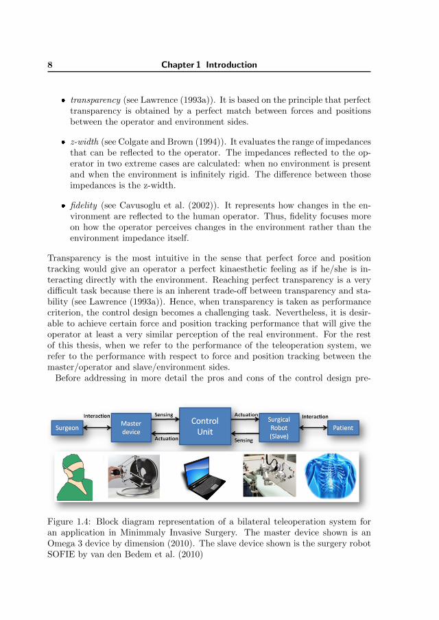
Before addressing in more detail the pros and cons of the control design pre-
Figure 1.4: Block diagram representation of a bilateral teleoperation system foran application in Minimmaly Invasive Surgery. The master device shown is anOmega 3 device by dimension (2010). The slave device shown is the surgery robotSOFIE by van den Bedem et al. (2010)

1.1 Bilateral teleoperation 9
sented in the literature, notice that in our block diagram representation in Fig. 1.4time delays are not included. Delays will always degrade the achievable perfor-mance of a system. In fact, already without delays obtaining high performanceand stability for a bilateral teleoperation system is a challenging problem. In thisthesis the research focus is on providing solutions towards closing the gap betweenperformance and stability of bilateral teleoperation systems. Hence, time delaysare deliberately not covered. Nevertheless, the reader can refer to Polat (2011),in which a similar framework as the one utilized in this thesis, is used to includetime delays in the control design.
1.1.4 Pros and cons of current bilateral control design methods
Passivity approaches
Passivity based methods are still widely used. A system is said to be passive if itdoes not generate energy. In particular, passive systems are asymptotically sta-ble. Moreover, if connected with other passive systems, the resulting system willalso not generate energy and thus will be passive as well. This modular propertyof passive systems has been exploited to generate the stability of teleoperationsystems. Indeed, if the operator and the environment are modelled as passivesystems, the interconnection with a passive teleoperator will result in a passiveteleoperation system. At this point there are two aspects which we would liketo discuss. Firstly, in the sense of the stability concept adopted here, a systemcan temporarily generate energy. In itself, this does not mean that the systembecomes unstable, provided that the states of the system remain bounded forbounded inputs. Thus, passivity is a property that can be used as a method toobtain stability of the system even if energy is supplied to the system. Secondly,there is an ongoing discussion on the passivity assumption of the operator, andrecent works suggest that the operator cannot be modelled as a passive systemfor all types of tasks (see, e.g., Polushin et al. (2012); Dyck et al. (2013); Polat(2014)). The operator can show passive behaviour while performing specific tasks,but shows non-passive behavior in performing others. For instance, the operatorcan choose to inject energy to the master device in order to perform his/her desiredmovements. Moreover, even if the operator would only show passive behaviour,modelling him/her as a passive system may add excessive conservatism. The setof dynamics covered by a passive system is much larger than the set of dynamicsthat an operator can show. For instance, an operator can not show the stiffnessof a piece of metal, which can be considered as a passive system. Nevertheless,passivity based methods can guarantee stability, but it does not take performanceexplicitly into account. Therefore, it does not provide the obvious mean to achievea systematic stability/performance trade-off. However, passivity can still be com-

10 Chapter 1 Introduction
bined with control design guidelines for performance. For instance, in Willaertet al. (2014) the authors have proposed methodologies that do take both perfor-mance and passivity requirements into account. They give guidelines to achievetransparency and passivity, at least in steady state, however the technique is lim-ited to master and slave devices with mass-damper-spring dynamics with identicalmechanical properties in both devices. They overcome this restriction by usingthe controller to also add dynamics on one of the devices, which will limit itsapplication if one of the devices has high damping or high mass. Moreover, inreal-life applications master and slave devices can have very different mechanicalproperties, which makes the technique limited in practice.
One important property of the operator and the environment, which is oftenoverlooked, is that they are inherently time-varying. However, some of the con-trol design tools based on passivity are valid only for Linear Time Invariant (LTI)passive systems, meaning that the operator and/or environment are additionallyassumed to be LTI. In fact, in many applications such as minimally invasive surgery(MIS), needle insertion, suturing etc., the environment varies over time in a certainbounded set, say in terms of varying stiffness properties. Moreover, many studieson the human arm dynamics have already shown that the human arm dynam-ics exhibits behaviour that can be covered by a model describing a bounded setof dynamics, see, e.g., Tee et al. (2004); Speich et al. (2005); Fu and Cavusoglu(2012). Therefore, the bilateral system interacts with a bounded environment anda bounded operator dynamics and the information of those bounds have not yetbeen fully exploited in the control design for teleoperation systems.
Researchers have proposed different methodologies to reduce the conservatismin stability analysis and control design for bilateral teleoperation systems. Currentmethods based on the passivity approach do not allow to incorporate uncertaintybounds, other than passive ones, for environment and operator in order to assessthe teleoperated system stability. This leads to a conservative methodology forbilateral control design. Indeed, previous works have presented absolute stabilitytests for a bounded uncertain environment based on passivity consideration, see,e.g., Willaert et al. (2009), Haddadi and Hashtrudi-Zaad (2010). In these testsconservatism is introduced via the operator model, which is taken to be passive.Additionally, the applicability of such stability criteria is limited since LTI envi-ronment uncertainties are assumed, which do not match the time-varying natureof the environment and operator dynamics.
Passivity in time
Some studies handle the passivity requirement in time-domain, see, e.g., Han-naford (2002), Ryu et al. (2004) and Franken et al. (2009). These works do takeinto account the time-varying nature of the bilateral teleoperation system. In those
1.1 Bilateral teleoperation 11
studies, the main method consists of calculating the energy flow of the system todetect when there is an energy build-up, and then apply the necessary forces toensure passivity. However, temporal generation of energy does not directly meaninstability of the system. According to the authors in Franken et al. (2009), thereis a separation in the control design for performance and stability. Nevertheless,the underlying controller could show active behaviour in order to achieve perfor-mance. Thus, the forces that would need to be applied to ensure passivity willhave an unknown effect on the performance. Moreover, in order to make a correctcomputation of the energy balance of the system, accurate models of friction forcesare needed, which in many real-life applications can be very difficult to obtain.
Robust control approaches
Other researchers have followed a different methodology based on robust control.For instance, Hu et al. (1995); Namerikawa et al. (2005), and Kim and Cavusoglu(2007), have addressed the robust performance control design using a structuredsingular value based approach. The environment/operator dynamics and uncer-tainties are considered as LTI systems, which approach will still not capture thetime-variations in a real physical setup. In Vander Poorten (2007), a scaled H∞norm method with constant scalings is utilized to handle the time-variations. How-ever, the authors already state themselves that “the fact that the usage of con-stant scaled H∞ guarantees robust interaction with any possible nonlinear andtime-varying system, might introduce a certain amount of conservatism”. Addi-tionally, virtual shunt dynamics are considered in order to obtain some bound onthe maximum operator impedance. However, bounds on the environment are notexploited, which can limit the achievable performance due to the large size of theuncertainty set. Alternatively, in Khan et al. (2009); Hace et al. (2011), slidingmode control is used to guarantee robustness, however, explicit information aboutthe bounded environment is not exploited and the performance is prone to typicalartifacts such as chattering behavior which degrades the operator’s feeling of theenvironment.
Approaches with adaptation to environment stiffness
Next, considering more realistic situations, there might be cases in which stiff en-vironments can be present. For instance, when performing an operation in MIS,there might be contact with bones, or it can be a collision between instruments.Thus, it is desirable to obtain high performance and stability in those cases as well.There is no guarantee that a single LTI controller exists that ensures both perfor-mance and stability for a large range of time-varying environment stiffness values.

12 Chapter 1 Introduction
To cover a large range of environment stiffness values, one can add flexibility in thecontrol design, for instance by means of estimating the actual environment stiff-ness and use such estimate to design a controller that adapts accordingly. Thisidea is not new and some works, e.g. by Hashtrudi-Zaad and Salcudean (1996);Love and Book (2004); Willaert et al. (2010); Cho et al. (2013), design controllersthat depend on the estimate of the environment stiffness. However, either they donot guarantee robust performance, or the achieved range of operation is limited tolow values of environment stiffness. Moreover, all of these works rely on accurate,unbiased, low noise and/or fast convergence of the estimated environment stiffness,requirements which in practice are difficult to meet simultaneously. Therefore, itis desirable that the limited performance of environment estimators is taken intoaccount during controller design. One approach that can be promising in pro-viding adaptation to the environment and does not rely on accurate estimates ofthe environment, is the use of switching control. For instance, multiple modeladaptive control has been used in teleoperation in Shahdi and Sirouspour (2005).The main underlying idea is to use different controllers under different kind ofenvironment stiffness, i.e. one controller for soft environments and another forstiff environments. The main issue in the implementation of the work presentedin Shahdi and Sirouspour (2005) is that at the moment of switching they obtainnon-smooth responses that can compromise the stability of the system. Moreover,in the controller design, uncertainty in the operator is not taken into account.
Applicability in real-life systems
Next, considering more practical aspects, most of the control approaches for bi-lateral teleoperation have been tested either only on academic setups, or in tele-operators with low masses and/or low friction. In practice, the force feedbackimplementation in teleoperators can be very challenging. The main reason is thatthe master and slave devices must meet specifications on, for instance, dimen-sions, degrees of freedom (DoFs), resistance and costs among others. This resultsin a number of mechanical limitations, e.g. high friction levels, heavy devices,structural resonances and lack of force sensors, limitations that in general are notpresent in academic setups that are commonly used in the literature to test bilat-eral controllers. Therefore, commercially available surgical systems do not haveforce feedback, e.g. the Da Vinci system (Guthart and Salisbury Jr (2000)), forwhich achieving force feedback is difficult due to the high masses involved (Shi-machi et al. (2008)). It is typical that these type of systems have a slave devicewith large mass, and a master device with low mass and without force sensors.Only few methods have been implemented and tested in such type of devices dueto the challenges involved (see, e.g., Beelen et al. (2013)). Thus, a systematic andpractically feasible methodology is needed.

1.2 Problem statement and challenges 13
This short literature survey covered the main control methodologies of interestbased on linear techniques, because the methods that will be presented here arealso based on linear techniques. However, we would like to mention that non-lineartechniques have similar issues as the linear techniques in what concerns mainly tooperator modelling. Most of the non-linear control techniques are based on pas-sivity, thus assuming passive operators and environments. Moreover, they focusmainly on the stability of the system, see, e.g., Nuno et al. (2011). Some authorshave extended control methodologies to include also non-passive behaviour, see,e.g., Polushin et al. (2012). Thus, due to the large class of dynamics covered,these techniques based on passivity deliver results that can add excessive con-servatism. Therefore, most of the motivation for the need of new modelling andcontrol approaches also holds for the non-linear case.
As a final remark, we would like to mention that the survey hereby provided, is byfar not complete, and many other areas of bilateral teleoperation have been leftout in order to focus on the problem that is treated here. For instance, there are alarge volume of active research focused on delayed teleoperation, on teleoperationvia the network, on multi-user teleoperation, etc.
1.2 Problem statement and challenges
After we reviewed the main control methodologies proposed in the literature, onecan conclude that there is still a number of challenges that demand research atten-tion. Therefore, an alternative approach towards bilateral control design is needed.In particular, there is a need to develop an approach that:
� takes explicitly into account the time-varying nature of operator and envi-ronment dynamics. A better characterization of those dynamics will help toguarantee that experimental results match better with the theory, improvingour understanding of bilateral teleoperation systems,
� allows for including information on the bounds of model parameters of theoperator and environment. This will narrow the set of dynamics for whichthe teleoperation system needs to have robust performance, thus less conser-vative results could be obtained,
� provides means to address performance and stability systematically. This willallow to specify a-priori the desired performance and stability properties ofthe teleoperation system and then design a controller that aims to achieveboth simultaneously,
� is suitable for master and slave devices with structural resonances and dif-ferent mechanical properties. Thus the technique can be applied in real-life
14 Chapter 1 Introduction
applications in which the master and slave devices are designed under a num-ber of specifications that results in limitations in their mechanical properties.
Moreover, in order to improve the performance in bilateral teleperation systems,it is desirable to have a control structure that additionally:
� provides adaptation to the environment dynamics when properly dealt with.This allows to increase the performance of the system,
� takes into account that environment estimators have limitations in accuracyand/or estimation noise and/or convergence speed. There is an inherenttrade-off between high accuracy, low noise and fast convergence in envi-ronment estimators. Thus, the controller should be designed to take thistrade-off into account.
1.3 Research approach
In order to provide a solution for the challenges previously mentioned, we adopt amodel-based robust control design approach. We will use a parametric model of theteleoperation system that captures the bounded dynamics present during normaloperation. To this end, for the human operator, we derive a parametric modelbased on identification experiments, thus characterizing a bounded set of dynamicsinspired by the mechanical properties of the operator’s arm. The environment canbe modelled according to the application of the bilateral teleoperation system. Forinstance, we consider environments in which stiffness is the dominant phenomenon,e.g. in stiffness palpation tasks present in surgery. In that case, the environmentstiffness is considered a parameter of the environment model. Subsequently, theparameters of both the environment and the operator models can be treated asparametric uncertainties. To account for realistic behaviour, those parametricuncertainties are considered to be bounded and time-varying. On the other hand,models for the master and slave devices can be identified using existing systemidentification techniques. Hence, the models of the components of the bilateralteleoperation system can then be incorporated into a model-based control designframework as depicted in Fig. 1.5, in which the uncertainty parameters can beisolated in a separate block ∆.
Closed loop system
In the representation of Fig. 1.5 we distinguish the following vector valued signals:
� q and p: define the signals through which model uncertainty is represented.

1.3 Research approach 15
Figure 1.5: Representation of a generalized plant model for an application inMinimmaly Invasive Surgery
� y: contains the measured signals. For instance, position and force signals.
� w: defines all disturbances and noises that influence the system’s perfor-mance. For instance, w contains sensor noise signals. We also include inw the signals representing the active forces from the environment and theoperator that act on the system. These signals perturb the position and theforce tracking of the system.
� u: defines the actuation signals of the system such as the actuation signalsof the master and the slave devices.
� z: defines the performance signals, e.g. position and force tracking errors.
Uncertainty specification
We aim to achieve robust stability of the system against the operator and theenvironment model uncertainties. We will use a specific class of Integral QuadraticConstraints (IQCs) (see Megretski and Rantzer (1997)) to model uncertainties∆ ∈ ∆. They allow to easily incorporate bounds and time-varying properties onthe uncertainty for control design. To this end, the class of dynamics ∆ of theuncertainty block ∆ can be represented by the IQC:
∫ T0
0
(∆(δ)q(t)q(t)
)TP
(∆(δ)q(t)q(t)
)dt ≥ 0 (1.3)

16 Chapter 1 Introduction
Specifically, let P = PT be a symmetric matrix of dimension [dim(p) + dim(q)]×[dim(p) + dim(q)] and suppose that p(t) = ∆(δ)q(t) in Fig. 1.5 where ∆ is anoperator ∆ : L2 → ∆L2 that has the property that Eq. (1.3) holds for all q ∈L2[0, T0], T0 ∈ R+.
The matrix P is a so called multiplier. Eq. (1.3) provides a generic way to representuncertainties. However, by itself it does not provide a means to find a specific classof matrices P that describes specific properties of the uncertainty ∆. Therefore, inorder to use Eq. (1.3), P needs to be classified or specified. There exists already anumber of multipliers that describe certain classes of uncertainties. To give somecommon examples, let us assume LTI uncertainties ∆. Then Eq. (1.3) is equivalentto: ∫ ∞
0
(∆(iω)I
)∗P
(∆(iω)I
)dω ≥ 0 (1.4)
Next, consider for instance the following multiplier
P =
(0 II 0
).
Then we have that
(∆(iω)I
)∗(0 II 0
)(∆(iω)I
)� 0 ∀ω ∈ R
∆(iω)∗ + ∆(iω) � 0 ∀ω ∈ R
which is equivalent to the positive realness of the uncertain system ∆, i.e. sameproperty as in passivity. In turn, this means that the uncertainty is modeled as apassive LTI system. Consider also
P =
(−I 00 I
).
With such a multiplier we have that (1.4) is equivalent to:
∆(iω)∗∆(iω) � I ∀ω ∈ R
which means bounded gain of the uncertain system, which can be used in combi-nation with the small gain theorem in a robust control framework. The multiplierP can describe mathematical properties of the uncertainties ∆. In our particularcase, we focus on a certain class of frequency independent multipliers that allowto characterize arbitrarily fast time-varying parametric uncertainties. This typeof characterization accounts for sudden changes of the environment and of theoperator dynamics.

1.3 Research approach 17
To illustrate how to find a proper matrix P that describes parametric uncertainties,consider the example in which we have a vector δ containing parametric uncertain-ties such that they are contained in a certain set δ. To not introduce conservatismin the uncertainty description via the IQC (1.3), ideally we need to find matrices Psuch that (1.3) holds only for δ ∈ δ. In practice, this can not always be achieved,thus approximations are used. For the case of bounded parametric uncertainties,we use the following procedure:
Consider the case when each of the Np uncertain parameters δi is time-varyingand bounded in the sense that δi : R+ → [δi, δi], for i = 1, ..., Np. Then, the
class δ =∏Np
i=1[δi, δi] is the uncertainty ‘cube’ in RNp which can actually bewritten as the convex hull of M = 2Np corner points δ1, ..., δM ∈ RNp . That is,δ = co{δ1, ..., δj , ..., δM}. For instance, if Np = 2 we will have that δ1 = col(δ1, δ2),δ2 = col(δ1, δ2), δ3 = col(δ1, δ2) and δ4 = col(δ1, δ2). Next, we assume that theuncertain parameters δi of the system can be included in the ∆ block of Fig. 1.5such that ∆(δ) = diag(δ1, ..., δNp).
Now, if both q and T0 are arbitrary in Eq. (1.3), it is then equivalent to:
(∆(δ)I
)TP
(∆(δ)I
)� 0 ∀δ ∈ δ (1.5)
One way to find a set P of symmetric matrices P that describes δ and satisfies(1.5) is the following: because of the convexity property of δ, it suffices to forceconcavity in the left hand side of (1.5) and evaluate (1.5) on the corner pointsδj , j = 1, . . . ,M that generate δ. Thus, we classify P by the matrices P such that
(∆(δj)I
)TP
(∆(δj)I
)� 0, j = 1, ...,M. (1.6)
and (I0
)TP
(I0
)� 0. (1.7)
These equations are the conditions that will allow to find a proper symmetric ma-trix P that will describe the class of bounded parametric uncertainties consideredin this thesis. For other ways to describe bounded parametric uncertainties, see,e.g., Megretski and Rantzer (1997); Scherer and Weiland (2000); Polat (2011).
Performance specification
The system’s representation in Fig. 1.5 allows to systematically incorporate per-formance and (robust) stability in the control design. The performance of the

18 Chapter 1 Introduction
system is quantified via a quadratic performance criterion from the disturbancesignals w to the performance signals z. Specifically, let Pp = PTp be a symmet-ric matrix of dimension [dim(w) + dim(z)] × [dim(w) + dim(z)] and consider theuncertain controlled system of Fig. 1.5. Suppose that z is uniquely defined by wfor all possible uncertainties ∆ ∈∆. Then we will say that the controlled systemachieves robust performance (or robust performance) if (1.8) holds for all w ∈ L2
and for all ∆ ∈∆.∫ ∞
0
(w(t)z(t)
)TPp
(w(t)z(t)
)dt < 0 ∀w 6= 0, (1.8)
Hence Pp describes a specific quadratic performance criterion. For instance, onecould state that passivity can be seen as a performance criterion for a certainsystem. Then, for the case that w and z are vector signals with one element,replacing
Pp =
(0 −I−I 0
)
in (1.8) results in ∫ ∞
0
w(t)T z(t)dt > 0 ∀w 6= 0. (1.9)
When w(t) and z(t) are defined such that they represent effort and flow variablesrespectively, (1.9) is equivalent to require that the total energy flow of the systemtrough the ports defined by w(t) and z(t) is positive, i.e. the same property as inpassivity (see Llewellyn (1952)).
Another example is the L2 gain of the mapping from disturbance signals to theperformance signals. Indeed, if we set
Pp =
(−γ2I 0
0 I
)
then (1.8) becomes ||z||22 < γ2||w||22 for all w ∈ L2. This performance criterion isequivalent to saying that
supw
||z||2||w||2
< γ, (1.10)
which for an LTI system it is equivalent to a bounded H∞. In Eq. (1.10), γ can beinterpreted as a worst-case gain from the disturbances to the performance signals.Therefore, instantaneous responses that can be felt by the operator have a directeffect on the performance criterion. This makes the L2 gain a suitable performancecriterion for teleoperation systems and it will be used as the performance criterionin this thesis.
One can see that other performance criteria can be also incorporated in the designby defining properly the matrix Pp, see, e.g., Scherer and Weiland (2000). Such

1.3 Research approach 19
flexibility in defining performance is one of the advantages of the framework utilizedin this thesis.
Robust stability and robust performance
The robust stability of the system is achieved if we obtain Input to State Stability(ISS) of the bilateral teleoperation system, as previously mentioned. The ISSconcept is based on the principle that for any initial condition x0 of the statevector x, and any bounded input u, there should exist some functions β ∈ KL andα ∈ K∞ such that
|x(t)| ∈ β(|x0|, t) + α(||u||∞) (1.11)
for all solutions x(t) of the system and for all t > 0. The classes KL and K∞are basically unbounded strictly increasing functions, the reader is referred to thework of Sontag (2008) for details. ISS is closely related to the concept of stabilityof dissipative dynamical systems. Here we present a brief conceptual descriptionon how such theory can be used to incorporate robust performance and stability.Let X be the state space of the state vector x of the system in Fig. 1.5. Let W andZ be the disturbance vector space and the performance vector space respectively.Let s : W × Z → R be a mapping (referred as the supply function) acting onall pairs (w, z) of the system. Then, the system with supply function s is said tobe robustly dissipative against time-varying uncertainties ∆ ∈ ∆ if there exists afunction V : X ×∆→ R such that
V (x(t1),∆(t1)) ≤ V (x(t0),∆(t0)) +
∫ t1
t0
s(w(t), z(t))dt (1.12)
for all t0 ≤ t1 and all signals (x,w, z,∆) that satisfy the system’s dynamics andall ∆ ∈ ∆. We call the function V a robust storage function. It expresses theamount of internal energy in the system when it finds itself in the state x ∈ Xand with uncertainty ∆ ∈ ∆. As a remark, the storage function V in (1.12) isnot required to be non-negative. However, for control design purposes, later wewill restrict ourselves to quadratic storage functions which are also non-negativein order to guarantee the system’s stability.
The concept in Eq. (1.12) can be interpreted as the requirement that a systemdissipates “energy” at a faster rate than the rate s(w, z) at which this “energy” isbeing supplied to it. In practice the “energy” quantity does not need to be literallythe energy of the system. For instance, in the performance specification section,different performance criteria were illustrated, which are directly related to thesupply function s(w, z). The quadratic performance specified by Pp describes thesupply function s. Thus, Pp will determine the corresponding type of “power”that is used.
20 Chapter 1 Introduction
It is beyond the scope of this thesis to enter into the details of the derivation of thecorresponding theory to get from the dissipation concept to tractable equationsuseful for control design. We will give a brief example on how this could beachieved. We restrict ourselves to Lyapunov functions of the form
V (x,∆) = xTXx,
i.e. V independent of ∆, and Lyapunov functions of the form
V (x,∆) = xTX (∆)x
with X = X T and X (∆) = X (∆)T being positive definite matrices. Consider wehave a system of the form:
x = A(∆)x+B(∆)w
z = Cx+Dw.
Then for t1 → t0 (1.12) is equivalent to :
∂V
∂xx ≤ s (1.13)
Considering also the supply function of the form s(w, z) = −[wz ]TPp[
wz ]. Then
(1.13) is equivalent to each of the following inequalities
2xTX (∆)(A(∆)x+B(∆)w) ≤ −(wz
)TPp
(wz
)
(x
A(∆)x+B(∆)w
)T (0 X (∆)X (∆) 0
)(x
A(∆)x+B(∆)w
)≤
−(
wCx+Dw
)TPp
(w
Cx+Dw
)
(xw
)T (I 0
A(∆) B(∆)
)T (0 X (∆)X (∆) 0
)(I 0
A(∆) B(∆)
)(xw
)≤
−(xw
)T (0 IC D
)TPp
(0 IC D
)(xw
)
which for arbitrary x ∈ X and w ∈W is equivalent to:
(I 0
A(∆) B(∆)
)T (0 X (∆)X (∆) 0
)(I 0
A(∆) B(∆)
)
+
(0 IC D
)TPp
(0 IC D
)� 0 (1.14)
1.3 Research approach 21
which is already a matrix inequality. Moreover, for specific cases of the dependencyon the uncertainty ∆, the inequality (1.14) can be expressed as a linear matrixinequality (LMI). In fact, for the trivial case that there is no dependency on theuncertainty ∆, (1.14) is already linear with respect to X . Hence, in that case itis said that (1.14) is an LMI. Therefore, it is possible to incorporate the perfor-mance and uncertainty specifications (which were already introduce as tractablemathematical conditions) in a series of linear matrix inequalities.
In fact, in the next chapters of this thesis, we will use the results from robustcontrol theory based on Linear Matrix Inequalities (LMIs)(see Scherer and Wei-land (2000)). These techniques are introduced and applied to the control designproblem.
Switching Control
Finally, to include adaptation to the environment properties, we propose the useof a multi-controller structure, in which we divide the environment dynamics insubregions, such that one controller covers each subregion. In this way, we do notrely on accurate estimates of the environment but only on a correct estimation ofthe subregion to which the environment currently belongs to.
Then for each subregion, we will design a LTI controller which presents robustperformance. The main challenge in such a multi-controller structure is to achieverobust stability of the overall system including the switching between its differentLTI controllers. We propose the use of three different switching techniques:
� based on the existence of a common Lyapunov function: It is known from theswitching systems theory (see Liberzon (2003)) that if different closed loopsystems have a common Lyapunov function, then arbitrary fast switchingamong those closed loop systems will result in a stable system. This ideais intuitive in the sense that the system will respect always the dissipationinequality in (1.12).
� based on average dwell time switching : In this concept, switching amongdifferent closed loop systems is restricted to a minimum average dwell timeτ (see Hespanha and Morse (1999)). This allows to use different Lyapunovfunctions for different closed loop systems, provided that the discrepancy ofthe different lyapunov functions is conditioned to a relation depending onthe average dwell time τ . In view of Eq. (1.12), in this case the times t0 andt1 are restricted with respect to τ and the overall Lyapunov function is thenallowed to increase temporarily.

22 Chapter 1 Introduction
� based on bumpless transfer : This concept was proposed by Zaccarian andTeel (2005) in order to activate a controller in a safe way. The main idea isto reduce the transient behavior at the moment that a certain controller is put‘on-line’ with a plant. This is achieved by virtually putting the controller ‘on-line’ before it is actually activated. To this end, the controller is simulated ina virtual loop and perturbed using signals measured from the real system. Inthis thesis we will adapt the bumpless transfer concept to perform switchingamong different robust controllers.
1.4 Contributions
Using the research approach previously described, in this thesis we present methodsand results that lead to contributions in the following areas:
Contribution 1. A systematic modelling and control design approach for bilat-eral teleoperation systems.The proposed approach uses an experimentally identified parametric model for theoperator and a pre-defined parametric model of the environment. The combinationof both models lead to a Linear Fractional Representation of the bilateral teleop-eration system. Then the parameters of the system are described explicitly astime-varying to account for realistic behaviour. Moreover, we describe how to userobust control synthesis techniques to design controllers with robust performanceunder time-varying dynamics in the operator and environment of the teleoperatedsystem. We provide guidelines on how to implement successfully such type ofcontrollers. This type of approach leads to a consistent theory, simulations andexperiment results.
Contribution 2. A gain-scheduling multi-controller structure with switchingbased on Lyapunov Function Conditions.This controller structure allows for different LTI controllers. Each controller isdesigned for a different range of environment stiffness, which leads to an improvedoverall performance of the teleoperated system. This structure is particularly use-ful when the environment stiffness varies within a wide range including soft andstiff environments. The main challenge is how to design the controllers to achievea smooth switching among them.Contribution 2.a. A gain-scheduling multi-controller structure with switchingbased on the existence of a common Lyapunov Function.The proposed method ensures smooth switching among controllers and improvesthe performance of the teleoperated system in comparison when a single LTI con-troller is used. The controller structure is also tested experimentally.Contribution 2.b. A gain-scheduling multi-controller structure with switching

1.5 Outline of the thesis 23
based on dwell time conditions.The proposed method presents stable switching among controllers under the as-sumption that the operator drives the system such that fast switching amongcontrollers is avoided. Simulation showed that the overall performance can beimproved with respect to the structure in contribution 2.a.
Contribution 3. A gain-scheduling multi-controller structure with switchingbased on Bumpless Transfer of Robust Controllers.The proposed structure allows for designing controllers independently for differentregions of environment stiffness. Stable switching is achieved by means of bump-less transfer. The structure is experimentally validated under regular operatingconditions.
Contribution 4. A controller design and implementation approach for a non-ideal teleoperator.We show how the model-based robust control techniques can be applied to teleop-erators with non ideal properties, e.g. high difference in dynamics of master andslave device, no force sensor or with structural resonances in the master device.
1.5 Outline of the thesis
This thesis is the compilation of several research works. The chapters are basedon journal or conference articles, which are either published or currently underreview. Because of this, there is partial overlap between the chapters.
Chapter 2This chapter addresses Contribution 1. It is based on the paper:
� Lopez Martınez, C. A., Polat, I., Molengraft, R. v. d., and Steinbuch, M.(2014e). Robust high performance bilateral teleoperation under boundedtime-varying dynamics. IEEE Transactions on Control Systems Technology.Accepted for journal publication
In this chapter, we propose a methodology in which we develop a parametric modelof the teleoperation system. Subsequently, we exploit robust control techniques todesign controllers that aim to achieve a predefined performance, and are robustto bounded but arbitrarily fast-time-varying parametric uncertainties. Analysis,simulation and experimental results shows the effectiveness of the method to trade-off perfect transparency and stability.
Chapter 3This chapter addresses Contribution 2.a. It is based on the paper:
� Lopez Martınez, C. A., Molengraft, R. v. d., and Steinbuch, M. (2014c).

24 Chapter 1 Introduction
Switching robust control for bilateral teleoperation. Under review for journalpublication
In this chapter we propose the synthesis of a switching robust controller that allowsto design multiple robust controllers suitable for different ranges of environmentstiffness, so that an overall better performance among a wide range of environ-ment stiffness is achieved. The controllers are scheduled using an estimate of theenvironment stiffness. We present synthesis, simulation and experimental resultsof the proposed approach, thus showing the effectiveness of the method to improvethe robust performance of the teleoperated system.
Chapter 4This chapter addresses Contribution 2.b. It is based on the paper:
� Lopez Martınez, C. A., Molengraft, R. v. d., and Steinbuch, M. (2014d).Switching robust control synthesis for teleoperation via dwell time condi-tions. In 9th International Conference, EuroHaptics 2014, Versailles, France.Springer. To appear online
In this chapter, we propose a method to further reduce conservatism in the achiev-able performance of switching robust control synthesis for teleoperation systems.In this approach multiple Lyapunov functions with a special structure are in-troduced, linked by conditions of minimum average dwell time switching amongcontrollers. We show the advantage of the proposed method by means of controlsynthesis and simulation for an 1-DoF teleoperation system.
Chapter 5This chapter addresses Contributions 3. It is based on the paper:
� Lopez Martınez, C. A., Molengraft, R. v. d., and Steinbuch, M. (2014a).High performance teleoperation by bumpless transfer of robust controllers.In IEEE Haptics Symposium 2014, pages 209–214, Houston, TX, U.S.A
In this chapter we propose a controller scheme with multiple robust controllers inwhich every controller is performance-optimized separately. The switching amongthem is based on bumpless transfer and they are scheduled using an environmentstiffness estimator. Limited accuracy and noise of such estimator is also takeninto account during control design. We show the applicability of the approach byexperiments on a 1-DOF teleoperated system.
Chapter 6This chapter addresses Contribution 4. It is based on the paper:
� Lopez Martınez, C. A., Molengraft, R. v. d., and Steinbuch, M. (2014b).Model based robust control for bilateral teleoperation: Applied to a non-ideal teleoperator. In preparation for journal publication
Design specifications in real-life applications of bilateral teleoperation, e.g. mini-mally invasive surgery, can impose a series of limitations on the master and slavedevices, e.g. lack of force sensors among others, resulting in non-ideal teleoper-

1.5 Outline of the thesis 25
ators, making the design and implementation of a bilateral controller very chal-lenging. In this chapter, we show how to implement model-based robust controltechniques in a surgical setup designed for robotic assisted surgery. The experi-mental results demonstrate that using a model based robust control methodology,high performance is achieved despite the limitations of the system.
Chapter 7In this chapter we draw the conclusions obtained from this thesis and recommen-dations for future works are given.

26

27
Chapter 2
Robust Bilateral Control underTime-Varying Dynamics
IN THIS chapter, we propose a methodology in which we develop a para-metric model of the teleoperation system. Subsequently, we exploit ro-
bust control techniques based on Linear Matrix Inequalities to design con-trollers that aim to achieve a predefined performance, and are robust tobounded but arbitrarily fast-time-varying parametric uncertainties. Wepresent analysis, simulation and experimental results of the designed con-troller, thus showing that the assumptions made during modeling are ap-propriate and the effectiveness of the method to trade-off perfect trans-parency and stability.
2.1 Introduction
Bilateral teleoperation systems allow an operator to manipulate a remote environ-ment by means of a master and a slave device with which a feeling of tele-presenceusing force feedback is obtained. The system is supposed to present high per-formance, e.g. the operator feels as if he/she is manipulating the environmentdirectly, in a stable fashion. However, there is an inherent trade-off between (ro-bust) stability and performance, see, e.g., Hannaford (1989); Lawrence (1993b),
This chapter is based on the following manuscript: Lopez Martınez, C. A., Polat, I., Molen-graft, R. v. d., and Steinbuch, M. (2014e). Robust high performance bilateral teleoperation underbounded time-varying dynamics. IEEE Transactions on Control Systems Technology. Acceptedfor journal publication

28 Chapter 2 Robust Bilateral Control under Time-Varying Dynamics
and it is a challenging problem to design controllers that meet an appropriate bal-ance, see, e.g. Hokayem and Spong (2006), Passenberg et al. (2010). Most of thecurrent design tools are based on passivity theory (Niemeyer and Slotine (1991)),which guarantees stability but does not provide a means to achieve systematicrobust stability/performance trade-off. Moreover, the dynamics of the environ-ment and the operator are inherently time-varying, which is a property that isoften overlooked, see Chapter 1 Section 1.1.4. Also, in many applications suchas minimally invasive surgery (MIS), needle insertion, suturing etc., the environ-ment varies in a certain range, say in terms of stiffness properties, e.g., 83 N/m forfat, up to 2483 N/m and so on (Gerovich et al. (2004)). Therefore, the bilateralsystem interacts with a bounded environment and bounded operator dynamicsand the information of those bounds have not yet been fully exploited in the con-trol design for teleoperation systems. In principle, this can lead to improve thesystem’s performance. Current methods based on the passivity approach requirethat the uncertain dynamics are passive for at least one of both the environmentor the operator in order to assess the teleoperated system stability. Therefore, analternative approach towards bilateral control design is needed, which allows usto incorporate bounds on the uncertainty of environment and operator dynamics.This will allow to reduce the conservatism for guaranteeing stability while meetingthe performance requirements, and at the same time, to take the time-varyingnature of teleoperation systems into account.
Researchers have proposed different methodologies to reduce the conservatism instability analysis and control design for bilateral teleoperation systems. Previousworks have presented absolute stability tests for a bounded environment, see, e.g.,Willaert et al. (2009), Haddadi and Hashtrudi-Zaad (2010). Such tests are non-conservative in terms of stability characterization based on Llewellyn’s absolutestability criteria (Llewellyn (1952)), however the modeling still introduces con-servatism due to the passivity assumption. Additionally, the applicability of thestability criteria in Willaert et al. (2009) and Haddadi and Hashtrudi-Zaad (2010)is limited since we have to assume that the uncertainties of the environment areLinear Time Invariant (LTI), which does not match the time-varying nature ofthe environment and operator dynamics. Some studies handle the passivity re-quirement in the time-domain, see, e.g., Hannaford (2002), Ryu et al. (2004) andFranken et al. (2009). In these studies, the authors ensure the stability of the bilat-eral system by forcing the involved model(s) of the teleoperation system to be pas-sive by explicitly monitoring the external behavior. The underlying controller thatis design for performance may show non-passive behavior. Thus, the forces thatare necessary to ensure passivity will have an unknown effect on the performance.Other works such as those by Hu et al. (1995); Namerikawa et al. (2005), and Kimand Cavusoglu (2007), have addressed the robust performance control design us-ing a structured singular value (SSV) based approach. The environment/operatordynamics and uncertainties are considered as LTI systems. This approach cannot

2.1 Introduction 29
capture the time-variations in the physical setup. In Vander Poorten (2007), ascaled H∞ method with constant scalings is utilized to handle the time-variations.However, the authors point out that “the fact that the usage of constant scaledH∞ guarantees robust interaction with any possible nonlinear and time-varyingsystem, might introduce a certain amount of conservatism”. Additionally, virtualshunt dynamics are considered in order to obtain some bound on the maximumoperator impedance. But again, bounds on uncertainty of the environment are notexploited, which can limit the achievable performance due to the large size of theuncertainty set. Alternatively, in Khan et al. (2009); Hace et al. (2011), slidingmode control is used to guarantee robustness, however, explicit information aboutthe bounded environment is not exploited and the performance is prone to typicalartifacts such as chattering behavior. This degrades the operator’s feeling of theenvironment.
We use a model-based robust control approach to controller design. We utilizemass-damper-spring models for the master and slave devices. For most applica-tions in bilateral teleoperation, such models are appropriate for describing theenvironment. For the human operator, we have constructed a parametric modelbased on identification experiments. Having a parametric structure for operatorand environment models, we can, then, extract the uncertain parameters to obtaina Linear Fractional Representation (LFR) of the teleoperation system. This rep-resentation allows to treat the uncertain parameters independently with separatebounds with ease (cf. Vander Poorten (2007)). Moreover, stability and perfor-mance specifications are addressed simultaneously via Linear Matrix Inequalities(LMIs). We describe the operator/environment uncertainty via a specific class ofIntegral Quadratic Constraints (IQCs) as in Megretski and Rantzer (1997). SuchIQCs allow to represent several types of uncertainty, including time-varying para-metric uncertainty, arbitrary fast or bounded rate uncertainty among others. Theyhave been previously used for stability analysis of teleoperation systems in Polatand Scherer (2012). Thus, in view of future works, IQCs offer great flexibility inuncertainty descriptions.
In this chapter, the synthesis of controllers that guarantee both performance andstability for a bounded range of time-varying environment and operator dynamicsis presented. To illustrate the design method, we consider environments in whichthe stiffness is the dominant phenomenon, e.g. in stiffness palpation tasks presentin surgery. Therefore, we assume an environment in which the stiffness is modeledto be bounded and time-varying at an arbitrarily fast rate. The latter aspectmodels the possibility of sudden changes in the environment stiffness, whereas themass and damping coefficients are fixed. For the operator dynamics, we use amodel that is based on a low-frequency approximation in which the stiffness isagain considered to be time-varying.
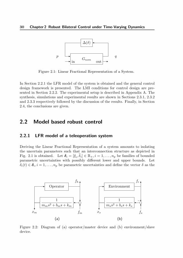
30 Chapter 2 Robust Bilateral Control under Time-Varying Dynamics
∆(δ)
Gnomp q
in out
Figure 2.1: Linear Fractional Representation of a System.
In Section 2.2.1 the LFR model of the system is obtained and the general controldesign framework is presented. The LMI conditions for control design are pre-sented in Section 2.2.2. The experimental setup is described in Appendix A. Thesynthesis, simulations and experimental results are shown in Sections 2.3.1, 2.3.2and 2.3.3 respectively followed by the discussion of the results. Finally, in Section2.4, the conclusions are given.
2.2 Model based robust control
2.2.1 LFR model of a teleoperation system
Deriving the Linear Fractional Representation of a system amounts to isolatingthe uncertain parameters such that an interconnection structure as depicted inFig. 2.1 is obtained. Let δi = [δi, δi] ∈ R+, i = 1, . . . , np be families of boundedparametric uncertainties with possibly different lower and upper bounds. Letδi(t) ∈ δi, i = 1, . . . , np be parametric uncertainties and define the vector δ as the
Operator
1
mms2 + bms+ km
fm
fh
xm
(a)
Environment
1
mss2 + bss+ ks
fs
fe
xs
−
(b)
Figure 2.2: Diagram of (a) operator/master device and (b) environment/slavedevice.

2.2 Model based robust control 31
vector of all np parametric uncertainties, that is, δ = col(δ1, . . . , δnp) ∈ Rnp . ∆(δ)
is the block diagonal mapping that acts on δ, i.e. ∆(δ) = diag(δ1, . . . , δnp). q and p
are the signals interfacing with the uncertainty block in the sense that p = ∆(δ)q.In particular, at any time instant t this means that p(t) = ∆(δ(t))q(t) is an ordinarymatrix multiplication. To derive the LFR model of the teleoperation system, theuncertainty parameters δ are defined and then isolated and collected into theuncertainty block ∆(δ). To this end, we first define the models of the differentcomponents of a teleoperation system. We focus on the particular mass-damper-spring models for master and slave devices, which interact with the operator andenvironment respectively as depicted in Fig. 2.2, where mm > 0, bm ≥ 0, km ≥0 are the fixed parameters of the master device representing its mass, dampingand stiffness coefficients respectively; similarly, ms > 0, bs ≥ 0, ks ≥ 0 are thefixed parameters of the slave device representing its mass, damping and stiffnesscoefficients respectively; fm, fs are the actuation forces to the master and slavedevices respectively; fh, fe represent the total force exerted by the operator andenvironment respectively; and xm, xs are the positions of the master and slavedevices respectively. By definition they also represent the positions of the operatorand environment respectively.
Environment model
We consider environments with mass-damper-spring dynamics:
fe = f∗e + (mexs + bexs + kexs), (2.1)
which models a significant class of applications of interest. Here, me ≥ 0, be ≥ 0and ke ≥ 0 are the mass, damping and stiffness coefficients of the environmentrespectively, and f∗e is the active force from the environment, if present. We focuson the environment stiffness ke as the main cause of the dynamic variation, henceme and be are assumed fixed and ke is assumed to be bounded and in additiontime-varying. That is 0 ≤ ke ≤ ke(t) ≤ ke for constants ke and ke. This choiceis suitable for applications in which the effect of ke on fe is dominant, e.g. instiffness discrimination tasks like those in surgery. For other environment types,Eq. (2.1), the uncertainty structure and parameters can be redefined. One shouldkeep in mind that because of the intrinsic robust stability/performance trade-off, it is expected that the greater the uncertainty set, the lower the achievableperformance. Finally, the coupled environment/slave-device system in Fig. 2.2bcan be represented as in Fig. 2.3, where the uncertainty block in this model isgiven, then, by ∆e = ke.

32 Chapter 2 Robust Bilateral Control under Time-Varying Dynamics
1s
1s
1ms
xsxsxs
me
be
ke
bs
ks
f∗e
fe
fs
Slave Device
Environment
−−
∆e
Figure 2.3: Block diagram representation of the environment/slave device pair.
Operator model
Next, in order to construct a realistic model for the operator, we identified exper-imentally the arm-hand dynamics of an operator while the operator manipulatedthe master-device of our experimental setup described in Appendix A, which hasbuilt-in force and position sensors. The operator dynamics are inherently time-varying and to obtain a time-varying model can be a difficult task. Instead, wesimply identify several LTI models and then we combine them into a time-varyingmodel. This works under the assumption that the operator can behave as an LTIsystem if he/she tries to remain static. We presented seven virtual springs to theoperator with stiffness values kVe ∈ [0, 5000] N/m such that fm = −kVe xm + f IDm ,in which f IDm will be used as a disturbance signal for system identification. Inparticular, we used a system’s sampling rate of 2000 Hz and a frequency range of[1, 30] Hz for the multi-sine. The block diagram used for the experiment is shownin Fig. 2.4. Initially we set f IDm = 0 N and then the operator was asked to movethe master device in order to feel the virtual spring. Subsequently, the operatorwas asked to stop in a position of his/her choice where he/she could still feel thevirtual spring. The idea is that the operator exerts a force level such that he/shecould feel that he/she has a correct haptic perception of the virtual environment.This is clearly subjective to the operator. Nevertheless, the aim of the experimentis that the operator changes intuitively his/her exerted force and grip for differentvirtual springs. Afterwards, a multi-sine signal was applied to the master devicevia f IDm while the operator tried to keep his/her hand-arm remain static. Forcesfh(t) and positions xm(t) were measured and then the corresponding Fourier trans-

2.2 Model based robust control 33
form Fmeash (jω) = F(fh(t))(jω) and Xmeas
m (jω) = F(xm(t))(jω) were computed.Next, we obtained the frequency response measurements of the static operator’sarm-hand dynamics as
Zmeash (jω) =
Fmeash (jω)
Xmeasm (jω)
for each virtual spring. All the resulting Frequency Response Measurements(FRFs) are depicted in Fig. 2.5. Based on the shape of those frequency domainmeasurements, for the static arm-hand dynamics Zh(s) we selected the modelstructure given in (2.2), where mh, bh, kh, are the mass, damping and stiffness ofthe human arm-hand, ωzh, zph and ωph are the parameters of the filter Qh(s) inEq. (2.3) which characterizes the operator dynamics above 10 Hz.
Zh(s) =Fh(s)
Xm(s)= (mhs
2 + bhs+ kh)Qh(s), (2.2)
where
Qh(s) =
s
ωzh+ 1
s2
ω2ph
+ 2zphs
ωph+ 1
(2.3)
Then, we optimized the variables mh, bh, kh, ωzh, zph and ωph to fit each measure-ment to the model minimizing the cost function WZh
(iω) = ‖Zh(iω)−Zmeash (iω)‖2
for ω ∈ 2π[1, 30] rad/s. The optimization is done using a constrained nonlinear op-timization method provided by the command fmincon in Matlabr. In practice theoptimization problem has several local minima, thus initial conditions and inter-val constraints must be provided to the solver. Those initial conditions and theirrespective constraints are estimated based on the measurements and are adjusteduntil a satisfactory match between Zh(iω) and Zmeas
h (iω) is obtained. The result-ing parameters were found to be within the following ranges; mh ∈ [0.39, 0.67] kg,bh ∈ [7.50, 9.66] N s/m, kh ∈ [649.54, 903.82] N/m, ωzh ∈ [62.85, 134.55] rad/s,zph ∈ [0.38, 0.59] and ωph ∈ [80.03, 94.59] rad/s. To reduce complexity of the
Operator
kVe
Master Device
fh
f IDmfm
xm
Figure 2.4: Diagram for arm-hand dynamics identification.
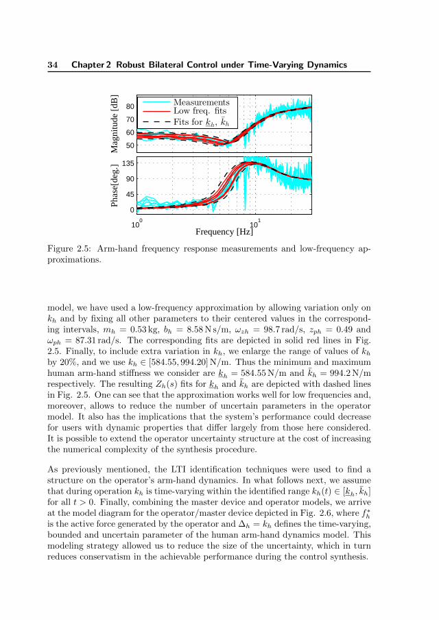
34 Chapter 2 Robust Bilateral Control under Time-Varying Dynamics
50
60
70
80M
agni
tude
[dB
]
100
101
0
45
90
135
Frequency [Hz]
Phas
e[de
g.]
MeasurementsLow freq. fits
Fits for kh, kh
Figure 2.5: Arm-hand frequency response measurements and low-frequency ap-proximations.
model, we have used a low-frequency approximation by allowing variation only onkh and by fixing all other parameters to their centered values in the correspond-ing intervals, mh = 0.53 kg, bh = 8.58 N s/m, ωzh = 98.7 rad/s, zph = 0.49 andωph = 87.31 rad/s. The corresponding fits are depicted in solid red lines in Fig.2.5. Finally, to include extra variation in kh, we enlarge the range of values of khby 20%, and we use kh ∈ [584.55, 994.20] N/m. Thus the minimum and maximumhuman arm-hand stiffness we consider are kh = 584.55 N/m and kh = 994.2 N/mrespectively. The resulting Zh(s) fits for kh and kh are depicted with dashed linesin Fig. 2.5. One can see that the approximation works well for low frequencies and,moreover, allows to reduce the number of uncertain parameters in the operatormodel. It also has the implications that the system’s performance could decreasefor users with dynamic properties that differ largely from those here considered.It is possible to extend the operator uncertainty structure at the cost of increasingthe numerical complexity of the synthesis procedure.
As previously mentioned, the LTI identification techniques were used to find astructure on the operator’s arm-hand dynamics. In what follows next, we assumethat during operation kh is time-varying within the identified range kh(t) ∈ [kh, kh]for all t > 0. Finally, combining the master device and operator models, we arriveat the model diagram for the operator/master device depicted in Fig. 2.6, where f∗his the active force generated by the operator and ∆h = kh defines the time-varying,bounded and uncertain parameter of the human arm-hand dynamics model. Thismodeling strategy allowed us to reduce the size of the uncertainty, which in turnreduces conservatism in the achievable performance during the control synthesis.
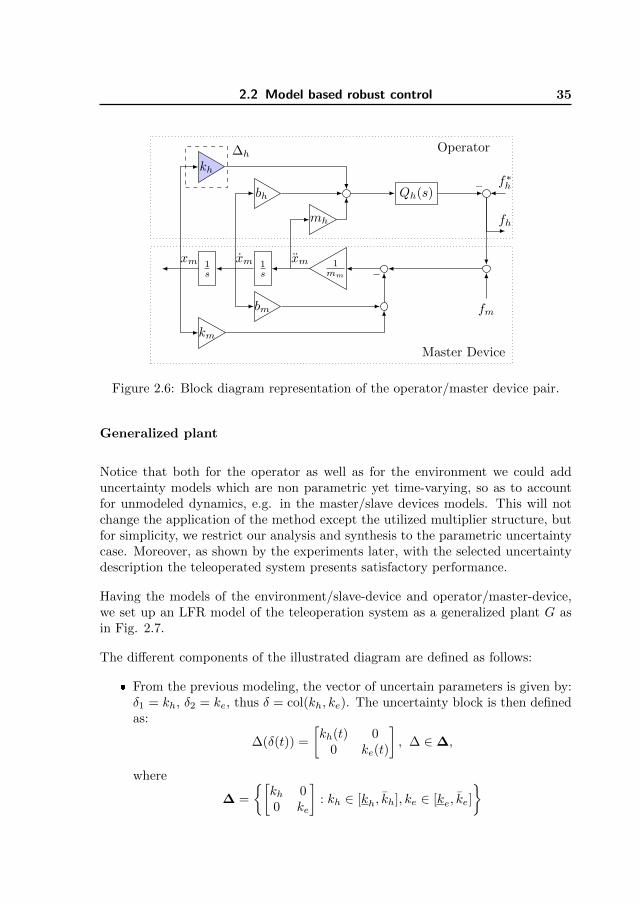
2.2 Model based robust control 35
1s
1s
1mm
xmxmxm
mh
bh
kh
bm
km
f∗h
fh
fm
Master Device
Operator
−
−Qh(s)
∆h
Figure 2.6: Block diagram representation of the operator/master device pair.
Generalized plant
Notice that both for the operator as well as for the environment we could adduncertainty models which are non parametric yet time-varying, so as to accountfor unmodeled dynamics, e.g. in the master/slave devices models. This will notchange the application of the method except the utilized multiplier structure, butfor simplicity, we restrict our analysis and synthesis to the parametric uncertaintycase. Moreover, as shown by the experiments later, with the selected uncertaintydescription the teleoperated system presents satisfactory performance.
Having the models of the environment/slave-device and operator/master-device,we set up an LFR model of the teleoperation system as a generalized plant G asin Fig. 2.7.
The different components of the illustrated diagram are defined as follows:
� From the previous modeling, the vector of uncertain parameters is given by:δ1 = kh, δ2 = ke, thus δ = col(kh, ke). The uncertainty block is then definedas:
∆(δ(t)) =
[kh(t) 0
0 ke(t)
], ∆ ∈∆,
where
∆ =
{[kh 00 ke
]: kh ∈ [kh, kh], ke ∈ [ke, ke]
}
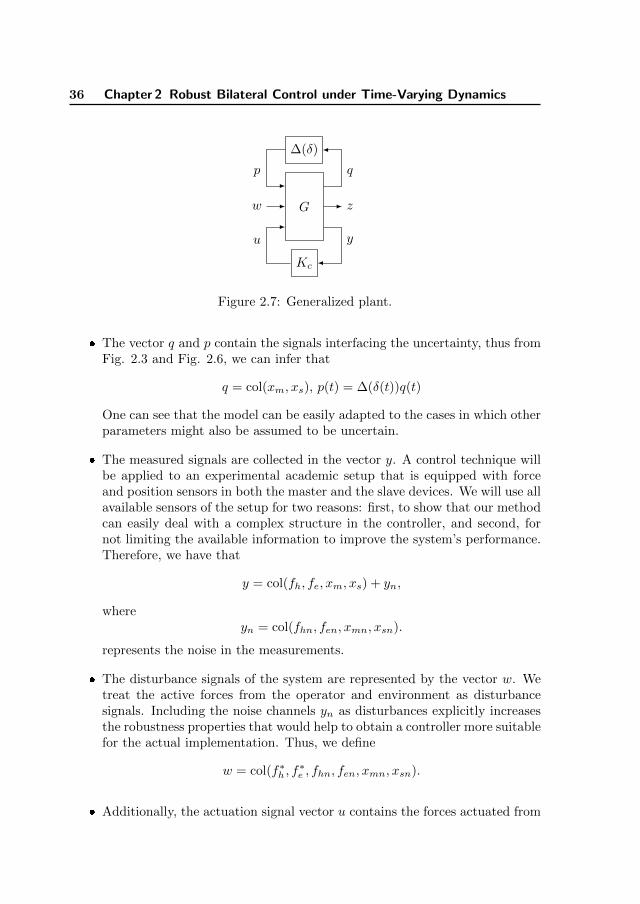
36 Chapter 2 Robust Bilateral Control under Time-Varying Dynamics
G
∆(δ)
Kc
w z
p
u
q
y
Figure 2.7: Generalized plant.
� The vector q and p contain the signals interfacing the uncertainty, thus fromFig. 2.3 and Fig. 2.6, we can infer that
q = col(xm, xs), p(t) = ∆(δ(t))q(t)
One can see that the model can be easily adapted to the cases in which otherparameters might also be assumed to be uncertain.
� The measured signals are collected in the vector y. A control technique willbe applied to an experimental academic setup that is equipped with forceand position sensors in both the master and the slave devices. We will use allavailable sensors of the setup for two reasons: first, to show that our methodcan easily deal with a complex structure in the controller, and second, fornot limiting the available information to improve the system’s performance.Therefore, we have that
y = col(fh, fe, xm, xs) + yn,
whereyn = col(fhn, fen, xmn, xsn).
represents the noise in the measurements.
� The disturbance signals of the system are represented by the vector w. Wetreat the active forces from the operator and environment as disturbancesignals. Including the noise channels yn as disturbances explicitly increasesthe robustness properties that would help to obtain a controller more suitablefor the actual implementation. Thus, we define
w = col(f∗h , f∗e , fhn, fen, xmn, xsn).
� Additionally, the actuation signal vector u contains the forces actuated from

2.2 Model based robust control 37
the motors of the master and the slave devices. Thus,
u = col(fm, fs)
� The performance vector z is defined as
z = col(fh − fe, xm − xs, fm, fs)
Via the component, fh − fe, we enforce that the human operator shouldfeel the same force applied by the environment. The second component,xm − xs, is the position error to obtain tracking between master and slave.The actuation variables are also included as channels to be penalized to avoidcontrollers with high gains.
� G is the model that contains all the fixed model dynamics of the differentcomponents of the bilateral teleoperation system: the master device, theslave device, the fixed operator dynamics and the fixed environment dy-namics if present. One can obtain a numerical model of G from the modeldiagrams presented in Figures 2.3 and 2.6 by making a partition as follows:
qzy
= G
pwu
where G is assumed to be LTI.
� Kc is the to-be-designed controller that maps the measured signals y to theactuation signals u.
The control design problem is then to find a controller Kc that achieves robuststability and robust performance for all ∆ ∈ ∆. At this point we still need todefine what structure the controller Kc will have and the type of performance thatis required from the system. This will be the subject of the coming sections.
Augmented generalized plant model for control design
The model presented in Fig. 2.7 is not suitable in its actual form for control design.Therefore, we augment the model such that the model that will be used for controldesign is illustrated in Fig. 2.8. The different components of the augmented plantare described as follows:
� V and W are weighting filters described with stable LTI systems. They allowto shape in frequency domain the desired system performance. These filters

38 Chapter 2 Robust Bilateral Control under Time-Varying Dynamics
G
T∆
∆(δ)
r
W
Kc
Vw zw z
u y
qp
p q
G
Figure 2.8: Generalized plant with weighting filters, uncertainty transformationand scaling. The dashed block in the upper part equals ∆(δ) provided r = 1.
will be defined in detail in Section 2.2.3. Meanwhile they are assumed to beknown.
� w and z are weighted copies of w and z via predefined filters V and Wrespectively. That is w = V w and z = Wz.
� δ is the vector of the transformed uncertain parameters δi ∈ δi, i = 1, . . . , np
such that δi = [δi, δi] ∈ R+ and 0 ∈ δi. Specifically, δ = col(δ1, δ2) =col(kh, ke), where kh ,ke are the transformed parameters corresponding tokh and ke respectively. In particular, we will use the following specific trans-formation functions to the parameters: In order to apply this procedure toour design case, we modify the loop such that the scaling r = 0 correspondsto the nominal case. We apply a transformation to the uncertainty parame-ters such that δi ∈ [δi, δi] are mapped to the uncertain parameters δi ∈ [0, 1],i = 1, . . . , np. This is achieved via the following transformations:
δi =δi − δiδi − δi
, i = 1, .., np (2.4)
� ∆(δ) is the block diagonal concatenation of the parameters in δ.
∆(δ(t)) =
[kh(t) 0
0 ke(t)
], ∆ ∈ ∆,
where
∆ =
{[kh 0
0 ke
]: kh ∈ [δ1,
¯δ1], ke ∈ [δ2,
¯δ2]
}
2.2 Model based robust control 39
� The vector q and p contain the signals interfacing the new uncertainty block∆. Thus p(t) = ∆(δ(t))q(t).
� r ∈ [0, 1]: is a scaling factor that allows to scale down the uncertainty block∆. This allows to perform an iterative process during the control designin which one starts with the nominal case r = 0, i.e. no uncertainty, andfinalizes with an unscaled uncertainty set for r = 1. We will refer to anominal plant if r = 0. If r = 1 we have that ∆(δ) equals the dashed blockin the upper part of Fig. 2.8.
� T∆ : R2np×2np is a constant matrix such that :(qp
)=
(r 00 1
)T∆
(pq
)
T∆ is used to map one to one the uncertain parameter set ∆ to the trans-formed uncertain parameter set ∆. The transformation T∆ allows to obtaina nominal value of ∆(δNom) ∈ ∆ for r = 0. The transformations applied tothe parameters in Eq. (2.4) can be achieved with the following transformationmatrix
T∆ =
(0 diag(δ1 − δ1, . . . , δnp
− δnp)
I diag(δ1, . . . , δnp)
)
One can construct a model of the generalized plant G by making the intercon-nection of blocks depicted in Fig. 2.8. The generality of the modeling procedureallows for adaptation to more complex linear dynamics of master and slave devices,other types of operator/environment models and other combinations of measuredvariables. Finally, we denote the state space representation of G by the followingequation:
xqzy
=
A B1 B2 BrC1 rD11 rD12 rE1
C2 D21 D22 E2
C F1 F2 0
xpwu
2.2.2 Robust control design with guaranteed performance spec-ifications
The common method for designing robust controllers is the use of multipliers tocharacterize the uncertainty and the performance specifications. It is also well-known that the overall robust control design is non-convex and, if exists, a con-vexifying procedure is not yet known. In the now-classic µ-synthesis framework

40 Chapter 2 Robust Bilateral Control under Time-Varying Dynamics
Skogestad and Postlethwaite (2005), it has been observed that an upper boundcomputation with an iterative algorithm is possible and tested extensively in prac-tice to conclude its validity. It is remarked that the resulting non-convex conditionsof the µ-synthesis framework can be shown to be bilinear in the unknowns and fix-ing a subset of unknowns renders the problem convex in the remaining ones. In thisfashion the multipliers and the to-be-designed controller are alternately fixed andat each step the uncertainty size is enlarged incrementally. This iterative schemehas originated from the µ-synthesis problem and since it deals exclusively with anorm bounded uncertainty type, the multiplier is typically denoted by D hencethe name D-K iteration. Along similar lines, µ-tools are extended to more generalcases and classes of multipliers have been reported in the literature Megretski andRantzer (1997), Polat (2011). In line with our experimental setup, we focus on aparticular uncertainty class, namely, the class of arbitrarily fast time-varying realparametric uncertainties.
Uncertainty description
We will use a specific class of Integral Quadratic Constraints (IQCs) (see Megretskiand Rantzer (1997)) to model uncertainties ∆ ∈ ∆. Then consider P as a set ofsymmetric matrices P ∈ R2np×2np that satisfy the following IQC
∫ T0
0
(∆(δ)q(t)q(t)
)TP
(∆(δ)q(t)q(t)
)dt ≥ 0 (2.5)
for all q ∈ L2[0, T0], T0 ∈ R+ and ∆ ∈ ∆.
The matrix P is a so called multiplier. It allows to describe mathematical proper-ties of the uncertainty block ∆. The set P needs to be further classified in orderto describe specific type of uncertainties. Thus Eq. (2.5) as such cannot be usedfor control design because we need first to formalize the relation between ∆ andP. If both q and T0 are arbitrary, condition in Eq. (2.5) is equivalent to
(∆(δ)I
)TP
(∆(δ)I
)� 0 ∀∆ ∈ ∆ (2.6)
Next, if the class ∆ is convex, it can be expressed as a convex combination ofgenerators δi, i = 1, . . . , 2np . In our specific case we have only four generators:
δ1 = col(δ1, δ2), δ2 = col(δ1,¯δ2), δ3 = col(
¯δ1, δ2) and δ4 = col(
¯δ1,
¯δ2). One way to
find a set P of symmetric matrices P that describes ∆ and satisfies (2.6) is thefollowing: because of the convexity property of ∆, it suffices to force concavityin the left hand side of (2.6) and evaluate (2.6) only at the corner points δj , j =

2.2 Model based robust control 41
1, . . . , 2np that generate ∆. Therefore, the convex class ∆ can be described by thenext finite number of inequality conditions:
(I0
)TP
(I0
)� 0 (2.7)
(∆(δj)I
)TP
(∆(δj)I
)� 0, j = 1, . . . , 2np (2.8)
where condition in Eq. (2.7) ensures concavity of the left hand side of condition inEq. (2.6). Therefore, the resulting P matrices classified by Eq. (2.7) and Eq. (2.8)imply that Eq. (2.6) holds.
In this case, P is then a constant full block multiplier describing bounded andtime-varying real parametric uncertainties. This is an important distinction ofthe methods in this thesis with those in Vander Poorten (2007), in which a morewider class of uncertainty is taken into account, which might add conservatism inthe achievable performance. Also notice that imposing structure and dynamics inthe matrix P , other types of uncertainty can be described as shown in Polat andScherer (2012), which can be exploited in future works.
Performance description
We have chosen the performance criterion based upon the L2 gain of the mappingfrom disturbance channels w to the performance channels z as is customary inmodel-based H∞ control, e.g., see Skogestad and Postlethwaite (2005). The L2
gain from w to z can be expressed as:
sup0 6=w∈L2
||z||2||w||2
< γ, (2.9)
in which γ can be interpreted as a worst-case gain from the disturbances w to theperformance signals z. Therefore, instantaneous responses that can be felt by theoperator have a direct effect on the performance criterion. This makes the L2 gaina suitable performance criterion for teleoperation systems.
The L2 gain can be expressed as a quadratic performance criterion: (2.9) is equiv-alent to each of the following conditions:
||z||22 < γ2||w||22 for all 0 6= w ∈ L2
∫ ∞
0
(w(t)z(t)
)TPp
(w(t)z(t)
)dt < 0 for all 0 6= w ∈ L2, (2.10)

42 Chapter 2 Robust Bilateral Control under Time-Varying Dynamics
with
Pp =
(−γ2I 0
0 I
)
In fact, it is possible to use other quadratic performance criteria, see, e.g., Sec-tion 1.3 and Scherer and Weiland (2000). To keep the generality of the theoryused here, we will use the symbol Pp to describe our performance criterion.
We proceed with the LMI-based robust controller design such that the closed loopis robustly stable and satisfies the performance specifications.
Robust Control Synthesis
We make use of an LTI controller Kc(s) = Cc(Is − Ac)−1Bc + Dc, which we willidentify with its state space description:
xc = Acx+Bcyu = Ccx+Dcy
.
by writing
Kc(s) =
[Ac BcCc Dc
].
We also introduce the shorthand notation for the closed loop matrices
G(s) ? Kc(s) =
A B1 B2
C1 D11 D12
C2 D21 D22
=
A+BDcC BCc B1 +BDcF1 B2 +BDcF2
BcC Ac BcF1 BcF2
r(C1 + E1Dc) rE1Cc r(D11 + E1DcF1) r(D12 + E1DcF2)C2 + E2Dc E2Cc D21 + E2DcF1 D22 + E2DcF2
obtained via closing the loop in Fig. 2.8 with the controller Kc(s).
We will utilize the following controller-multiplier iteration method: Let P be theset of symmetric matrices P that satisfy conditions (2.7) and (2.8) and assume wehave a controller Kc(s) that achieves nominal stability;Theorem 2.1. The closed loop system G(s) ? Kc(s) with r ∈ (0, 1] shown inFig. 2.8 is robustly stable for all ∆ ∈ r∆ with a guaranteed performance charac-terized by Pp if there exist a symmetric matrix X and P ∈ P such that
X � 0 (2.11)

2.2 Model based robust control 43
and
(?
)T
0 X 0 0X 0 0 00 0 P 00 0 0 Pp
I 0 0A B1 B2
0 I 0C1 D1 D12
0 0 IC2 D21 D2
≺ 0 (2.12)
holds.
For notational convenience we also introduce the partitions
P =
(Q SST R
), Pp =
(Qp SpSTp Rp
).
where Q,R, S ∈ Rnp×np , Qp ∈ Rdim(w)×dim(w), Sp ∈ Rdim(w)×dim(z) and Rp ∈Rdim(z)×dim(z).Remark 2.2. Theorem 2.1 allows to do analysis of robust performance of the sys-tem given a controller Kc(s). Then all the involved conditions are LMIs. However,in the case of controller synthesis, there is an issue. In (2.12), the outer factorsinvolving the state-space matrices of Kc(s) multiply the blocks of the multiplierinvolving unknown variables rendering the constraint a Bilinear Matrix inequal-ity (BMI). Nevertheless, by means of the transformations that have been given inScherer and Weiland (2000); Masubuchi et al. (1998); Scherer. et al. (1997), it ispossible to make (2.12) an LMI when P is fixed. Moreover, Ac, Bc, Cc, Dc matricesalso multiply each other, hence a linearization is needed. Fortunately, this can beavoided with a Schur complement argument.
Initially, we have neither a controller nor a multiplier by which the constraintsare satisfied. Hence one typically starts with the nominal system Gnom = 0pq ? G(which is an upper LFT and equivalent to removing the uncertainty channels).Then it is well-known how to design a nominally stabilizing controller (i.e. r = 0)with certain performance level. This makes it possible to search for a feasiblemultiplier via Theorem 2.1. Obviously, we can not expect a robust stability cer-tificate from the initial controller Knom since there is no constraint enforcing it.Thus, we need to first scale down uncertainty size to the level that Knom robustlystabilizes the system. This scaling (often simply a gain) can be subsumed into theuncertainty channels of the closed loop plant. Then by a line search over the fea-sible uncertainty size denoted by r ∈ (0, 1], we obtain feasible stability multipliers.Then, we switch to the controller step of the iteration.
As we pointed out in Remark 2.2, there exists a transformation such that theconditions in Theorem 2.1 are converted into LMIs, such transformation is brieflyreplicated here for completeness. The main difficulty with the bilinear terms in
44 Chapter 2 Robust Bilateral Control under Time-Varying Dynamics
(2.12) is resolved by changing the search over the variables from X , Ac, Bc, Cc, Dc
to another derived set of variables v = {X,Y,K,L,M,N} where X is the leftupper block of X , Y is the left upper block of X−1 and
(K LM N
)=
(U XB0 I
)(Ac BcCc Dc
)(V T 0CY I
)
+
(XAY 0
0 0
)(2.13)
which results from a congruence transformation which is omitted here but detailedin Scherer and Weiland (2000). Hence the closed loop state-space matrices become
(A(v) Bj(v)
Ci(r, v) Dij(r, v)
)
=
AY +BM A+BNC Bj +BNFjK AX + LC XBj + LFj
ri(CiY + EiM) ri(Ci + EiNC) ri(Dij + EiNFj)
(2.14)
for i, j = 1, 2 with r1 = r and r2 = 1. Finally, the positivity constraint on X � 0becomes
X(v) =
(Y II X
)� 0 (2.15)
In summary, following result gives the conditions for a stabilizing controller withguaranteed performance levels. Note that it boils down to verifying (2.12) in adifferent set of variables. For convenience we will omit the v and r dependencefrom the boldface variables.Theorem 2.3. There exists a controller Kc(s) and a Lyapunov certificate X suchthat the closed loop is robustly stable against all ∆ ∈ r∆ with r ∈ (0, 1] with Ppperformance if and only if there exist variables v such that X � 0 and
(?
)T
0 0 0 I 0 00 Q 0 0 S 00 0 Qp 0 0 SpI 0 0 0 0 00 ST 0 0 R 00 0 STp 0 0 Rp
I 0 00 I 00 0 IA B1 B2
C1 D1 D12
C2 D21 D2
≺ 0 (2.16)
hold.
At this point, (2.16) is not still an LMI since boldface variables enter quadratically,however it suffices to apply the Linearization Lemma described in Scherer andWeiland (2000) to render it as an LMI; having zero in the parameter intervals

2.2 Model based robust control 45
implies R,Rp � 0 and hence we can find a factorization Tl such that
(Ql + SlBl(v) +Bl(v)TSTl Bl(v)TTl
TTl Bl(v) −Ul
)≺ 0 (2.17)
where
Bl(v) =
A(v) B1(v) B2(v)C1(v) D1(v) D12(v)C2(v) D21(v) D2(v)
Ql = diag(0, Q,Qp)
Sl = diag(I, S, Sp)
Ul = diag(I,R−1, R−1p )
Tl = diag(0, I, I)
Constraint (2.17) is now affine in the variables v. After solving for v, the controllerparameters can be recovered by solving (2.13) for the original variables
(Ac BcCc Dc
)
=
(U XB0 I
)−1(K −XAY L
M N
)(V T 0CY I
)−1
where U and V are arbitrary invertible matrices satisfying I−XY = UV T . In ourcase we have selected U = X and V = X−1 − Y . Clearly we assume the existenceof a nominal controller that provides an initial condition for the first iteration thatwill not lead to a local minimum very close to r = 0, which in practice is actuallythe case. To summarize, we start with the design of a nominal controller designedfor r = 0. Then, we iterate the following two steps:
� for a fixed controller Kc(s), maximize r using the bisection algorithm andget the multiplier P , while optimizing for the Pp.
� for a fixed P matrix, maximize r using the bisection algorithm and get thecontroller Kc(s) while optimizing for the Pp.
The procedure is stopped when either, no further progress on increasing r < 1, orwhen r approaches 1 with the desired accuracy. Details on the iterative procedureare given in Appendix B, from which we have used the version I of the iterativeprocedure.
In the next section we describe how to translate the performance specifications viaweighting filters W and V .

46 Chapter 2 Robust Bilateral Control under Time-Varying Dynamics
2.2.3 Weighting filter design
In robust control design it is customary to implement frequency dependent weightson the performance channels (Fig. 2.7). The filters V and W are block diagonaltransfer matrices emphasizing the frequency band in which we want the particularchannel to be penalized. Thus V = diag(Vf∗h , Vf∗e , Vfhn
, Vfen , Vxmn , Vxsn) and W =diag(Wfh−fe ,Wxm−xs
,Wfm ,Wfs). Ideally, one wants to have fh − fe = 0 andxm − xs = 0. In this case we would get perfect transparency, but as is known,this type of design is unrealistic and has poor stability properties. Instead, it isdesirable to relax such a strict requirement by appropriate choices of V and W .
Instead we are interested in forcing the force and position tracking errors such thatin frequency domain |Fh(ω)−Fe(ω)| < γ|Fw(ω)| and |Xm(ω)−Xs(ω)| < γ|Xw(ω)|,where Fh(ω), Fe(ω), Xm(ω), Xs(ω) are the Fourier transform of fh, fe, xm,xs re-spectability, Fw(ω) and Xw(ω) represent the desired level of force and positiontracking in the frequency band of interest and γ > 0 is as small as possible. We as-sume |Fw(ω)| > 0 and |Xw(ω)| > 0 sufficiently small at low frequencies to achieveforce and position tracking for sufficiently slow varying forces and positions. Thiswill lead to a desired level of performance in the frequency range in which the hu-man operator performs movements. On the other hand, we need to have feasiblecontrol action with magnitude bounded forces fm, fs and a reduced amplificationof disturbance w to z at high frequencies. This to avoid saturation and the ex-citation of high frequency dynamics. These requirements are translated into thefilters W and V which are shaped accordingly. To illustrate how to achieve this,consider the design of a controller Kc for the nominal plant. Suppose that, forgiven V , W this leads to:
supw
||W (s)(G(s) ? Kc(s))V (s)w||2||w||2
< γ.
for some, preferably small, value of γ > 0. In the LTI case then we have that
||W (s)(G(s) ? Kc(s))V (s)||∞ < γ,
where || · ||∞ denotes the H∞ norm. In particular, this implies that the (m,n)thentry of W (s)(G(s) ? K(s))V (s) satisfies
|Wn(iω)(G(iω) ? K(iω))mnVm(iω)| < γ,
for which non-zero W , V implies that
|(G(iω) ? K(iω))mn| <γ
|Wn(iω)Vm(iω)| .
Hence, with γ > 0 fixed, frequencies at witch V and W have higher magnitude,will result in frequencies at which G(s)?Kc(s) has smaller magnitude and therefore

2.2 Model based robust control 47
Mag
nitu
de
ωbw
clf2
cxcs2
1
cxcs2
∣
∣
∣
∣
1
Wxm−xs
∣
∣
∣
∣
Frequency (rad/sec)
Mag
nitu
de
ωlp ωrf
1
cs3
ωlp
cs3ωr
∣
∣
∣
∣
1
Wfm
∣
∣
∣
∣
Figure 2.9: Magnitude bode plot of 1/Wxm−xs and 1/Wfm .
less amplification from w to z. This property can actually be employed to definethe filters V and W per frequency of interest.
We translate the performance specifications by defining the following filters:
Wfh−fe(s) =
cs1
s
ωbw+ 1
s
ωbw+ clf1
2
Wxm−xs(s) = cxscs2
s
ωbw+ 1
s
ωbw+ clf2
Wfm(s) = Wfs(s) = cs3
s
ωlp+ 1
s
ωr+ 1
Vf∗h = Vf∗e = cs4
Vfhn= Vfen = cs5
Vxmn= Vxsn
=cs6cxs

48 Chapter 2 Robust Bilateral Control under Time-Varying Dynamics
Typical shapes of the magnitude-bode plots |1/Wxm−xs(iω)| (which has a similar
shape as |1/Wfh−fe(iω)|) and |1/Wfm(iω)| (which the same shape as |1/Wfs(iω)|)are shown in Fig. 2.9.
ωbw defines the desired closed-loop bandwidth, ωlp defines the desired bandwidthof the actuation force signals. With the values clf1, clf2 we put a limit to Wfh−feand Wxm−xs at low frequencies. This also ensures the filters Wfh−fe and Wxm−xs
to be stable. Stability of all filters is necessary to ensure that a stabilizing controllerKc exists for the guaranteed plant. A second order filter was selected for Wfh−feto increase the tracking performance obtained in practice. On the other handfor Wxm−xs
a first order filter was sufficient. To avoid non-causal Wfm and Wfs ,we inserted high frequency poles at ωr. Moreover, cxs is used to scale penaltieson positions with respect to penalties on forces. This makes the magnitude ofpositions and forces numerically comparable. To keep the tuning more intuitively,cxs is tuned independently and it is not integrated into the scaling cs2 in Wxm−xs
.Finally, cs1, . . . , cs6 are scaling constants that are used for further tuning.
The structure of the weighting filters was designed to achieve position and forcetracking. However, other choices may be explored. For instance, one can addan intermediate impedance between the positions and forces of environment andoperator to mimic a “mechanical tool” as described in Vander Poorten (2007) inwhich again perfect transparency is avoided. This can be achieved by adapting Vand W .
2.3 Robust control applied to a 1-DoF academic setup
The potential of the synthesis method described above is demonstrated by applyingit to the experimental setup described in Appendix A. We demonstrate the robustperformance properties of the Robust Controller (hereafter referred to as RC) bymeans of simulations and experiments under operating conditions of permanentcontact with springs and sudden changes of environment stiffness.
Using frequency response measurements, the parameters of second order modelsfor the devices of the 1-DoF setup are identified. The parameters are listed inTable 2.1. In the same table we show the parameters of the operator and theenvironment dynamics that are computed at the end-effector. We have selectedke ∈ [80, 3000] N/m because we aim to guarantee performance and stability forenvironment stiffness values in the range of soft tissue environments.

2.3 Robust control applied to a 1-DoF academic setup 49
2.3.1 Synthesis results
The numerical parameters of the weighting filters are selected as follows. We haveselected ωbw = 2π× 10 rad/s as the desired closed loop bandwidth. The actuationforces fm, fs were penalized from 60 Hz and beyond, hence ωlp = 2π × 60 rad/s.clf1 and clf2 are selected to be small shifts to the poles at the origin to renderthe corresponding filters stable, i.e., clf1 = clf2 = 10−2 and ωr = 2π × 500 rad/s.We assume that the bandwidth of the actuators and sensors is higher than ωlp,so that stability is not compromised. In fact this assumption is validated by theexperiments. Next, the scaling cxs corresponds to the scaling between the forcesin the disturbance channels and the positions in the performance channels. Now,to estimate the order of such scaling, assume that we indeed achieve perfect forceand position tracking, therefore we can assume that the scaling between fh andpositions is equivalent to the environment stiffness. Because the force due to thearm-hand dynamics opposes to the force f∗h (Fig. 2.6), cxs is expected to be biggerthan the environment stiffness. Therefore the ke can be used as a lower bound forcxs > 3000(0.075)2 = 16.9. Note that the end-effector length is included since theinternal parameters are computed at the rotational axis. We have further tunedexperimentally by increasing it until satisfactory results were obtained, which ledus to the value cxs = 31.6.
The scaling parameters cs1, . . . , cs6 are tuned iteratively with the design process.We start with all values at 1, i.e. no scaling. The synthesis process is run and ifno controller is found or the results are not satisfactory, e.g. factor r is too small,we relax the penalization on the actuation variables by decreasing cs3. In casewe still do not make progress, then we start relaxing the penalization on one (ormore) performance variable(s) by decreasing the respective scaling parameter(s),depending on where we want to sacrifice performance, for instance by decreasingcs6 we allow for more position-sensor noise amplification. We iterate on the pre-vious steps to obtain finally the values cs1 = 0.56, cs2 = 0.5, cs3 = 0.4 cs4 = 1,cs5 = 0.5 and cs6 = 0.25. We have included low-pass filters with a bandwidth of
Table 2.1: Numerical parametersm′m = 1.36× 10⁻³ m′s = 1.29× 10⁻³ kg m2/radb′m = 1.01× 10⁻¹ b′s = 6.02× 10⁻² N m s/radk′m = 1.75 k′s = 0.46 N m/radmh = 0.53 me = 0 kgbh = 8.58 be = 0 N s/mkh ∈ [584.6,994.2] ke ∈ [80,3000] N/mωph = 87.31 ωzh = 98.7 rad/szph = 0.49 −
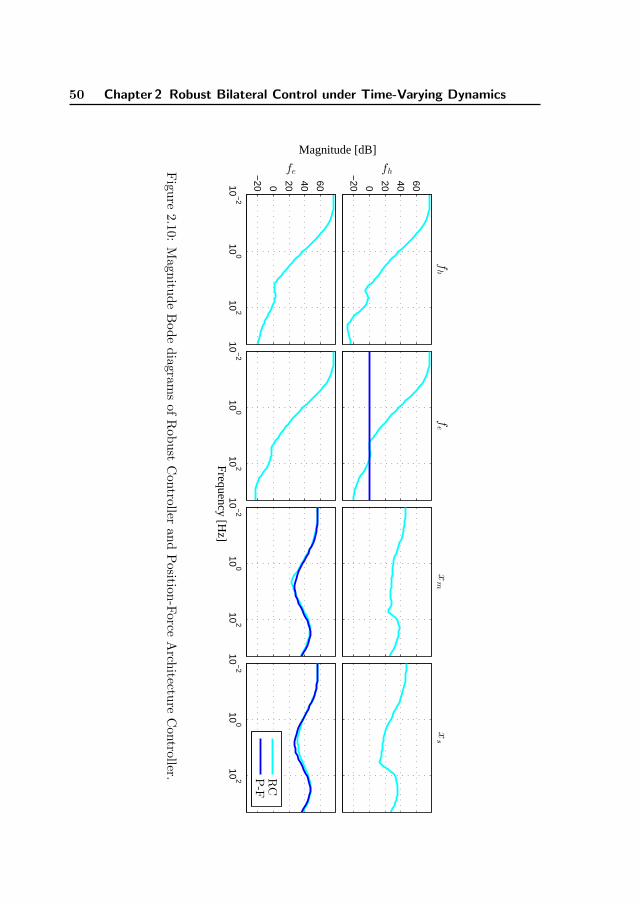
50 Chapter 2 Robust Bilateral Control under Time-Varying Dynamics
Frequency [Hz]
Magnitude [dB]
10−
210
010
2
10−
210
010
210
−2
100
102
10−
210
010
2
−20 0 20 40 60
fe
xs
xm
fe
−20 0 20 40 60
fh
fh
RC
P-F
Figu
re2.10:
Magn
itude
Bod
ed
iagrams
ofR
obu
stC
ontroller
an
dP
ositio
n-F
orce
Arch
itecture
Con
troller.

2.3 Robust control applied to a 1-DoF academic setup 51
200 Hz to the output signals y which are implemented in the experimental setup.
We limit our focus to the case when the operator is grasping the device, however,this leaves out the case when the user releases the master device, for which onlystability is relevant. Roughly speaking, when the operator releases the device, thetotal mass of the system decreases, increasing the open-loop gain and possiblycompromising stability. Instead of increasing the number of uncertain parametersto cover the release case in a conservative fashion, we utilize an alternative prag-matic approach. It consists in making the design using a reduced but fixed valueof mh = αmN
h for 1 > α ≥ 0 such that the system is stable in free air. Underthe previous assumptions, the synthesis algorithm was performed. The LMI’s forcontroller synthesis were solved using the solver SeDuMi Sturm (1999). We startedfrom α = 0 and we increased it by steps of 0.1. For each tested α, the desiredscaling value r = 1 was achieved using the algorithm described in Appendix B.2.We stopped increasing α when stability of the system in free air was not satisfied,which was verified analytically and also experimentally. In this fashion, we tookthe penultimate tested α. Therefore we finally used mh = 0.4mN
h . The gammavalues and scalings obtained at each controller/multiplier iterations for the finaldesign are shown in Table 2.2. As a remark, the order of the controller is the orderof the generalized plant G, which already includes the weighting filters. In ourcase, the controller is of order 15, the respective magnitude Bode diagram of theRC is shown in Fig 2.10.
In Table 2.2, one can see that during the synthesis process, a minimal L2-gain per-formance γ = 4.86 is achieved for the desired ranges of environment and operatorparameters. That is, feasibility of the synthesis LMIs for (α, r, γ) = (0.4, 1, 4.851).This design was made for α = 0.4, however the performance can be different forthe more realistic mass value α = 1. To illustrate the performance decrease, wealso analyze the performance using the obtained generalized plant (including theweighting filters) in closed loop with the designed controller. Such analysis canbe done by minimizing γ while solving the LMI’s of Theorem 2.1. We did two
Table 2.2: γ and r during iterations of the final designIter. r γ Kc/P
1 0 2.391 Kc
2 0.141 3.443 P3 0.382 3.966 Kc
4 0.556 3.808 P5 0.792 4.386 Kc
6 0.883 4.211 P7 1.0000 4.851 Kc

52 Chapter 2 Robust Bilateral Control under Time-Varying Dynamics
500 1000 1500 2000 2500 3000 3500 4000
10
100
1000
ke [N/m]
γ
RC (α = 0.4)
RC (α = 1)
P-F (α = 1)
P-P (α = 1)
Figure 2.11: Weigthed L2-gain performance analysis with different controllers forincreasing maximum environment stiffness ke
performance analysis of the obtained RC, one for α = 0.4 used during synthesis,and another for α = 1. The resulting γ values as a function of ke are given in Fig.2.11.
When α = 0.4, one can see that we obtain γ ≈ 5 for ke≤ 3000 N/m as alreadyexpected from Table 2.2. On the other hand, when the analysis is done for α = 1,which better describes the real system behavior during normal operation, γ in-creases for increasing values of ke, i.e. there is a bigger influence of the disturbancesignals on the performance channels hence a degradation of the overall perfor-mance. Notice that unfortunately, there is no one to one correspondence betweenthe γ values and the resulting performance. This is because γ is the worst-case L2
gain from the weighted inputs to the weighted outputs. Therefore γ is a relativeand not absolute measurement.
For α = 1 and 0ke> 2500 N/m no feasible γ was found. Since our test is onlysufficient, and it accounts for arbitrarily fast time-varying uncertainty, infeasibilityfor all values of γ in this analysis results means that there might exist a series ofdriving signals and time-varying change in environment that can destabilize thesystem. However, we were not able to destabilize the system when tested withenvironment stiffness values up to ke≈ 3000 N/m, as shown in the simulations andexperimental results.
Finally, we performed a similar performance analysis with α = 1 to other well-known architectures for bilateral teleoperation: “position-position” (P-P) archi-tecture, “position-force” (P-F) architecture and “transparent four-channel” (T4C)
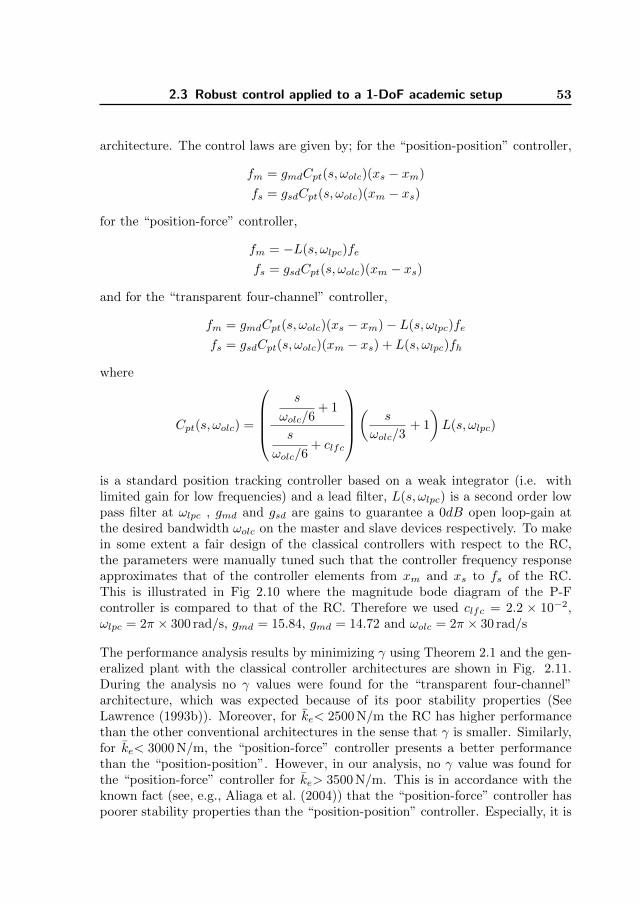
2.3 Robust control applied to a 1-DoF academic setup 53
architecture. The control laws are given by; for the “position-position” controller,
fm = gmdCpt(s, ωolc)(xs − xm)
fs = gsdCpt(s, ωolc)(xm − xs)
for the “position-force” controller,
fm = −L(s, ωlpc)fe
fs = gsdCpt(s, ωolc)(xm − xs)
and for the “transparent four-channel” controller,
fm = gmdCpt(s, ωolc)(xs − xm)− L(s, ωlpc)fe
fs = gsdCpt(s, ωolc)(xm − xs) + L(s, ωlpc)fh
where
Cpt(s, ωolc) =
s
ωolc/6+ 1
s
ωolc/6+ clfc
(s
ωolc/3+ 1
)L(s, ωlpc)
is a standard position tracking controller based on a weak integrator (i.e. withlimited gain for low frequencies) and a lead filter, L(s, ωlpc) is a second order lowpass filter at ωlpc , gmd and gsd are gains to guarantee a 0dB open loop-gain atthe desired bandwidth ωolc on the master and slave devices respectively. To makein some extent a fair design of the classical controllers with respect to the RC,the parameters were manually tuned such that the controller frequency responseapproximates that of the controller elements from xm and xs to fs of the RC.This is illustrated in Fig 2.10 where the magnitude bode diagram of the P-Fcontroller is compared to that of the RC. Therefore we used clfc = 2.2 × 10⁻²,ωlpc = 2π × 300 rad/s, gmd = 15.84, gmd = 14.72 and ωolc = 2π × 30 rad/s
The performance analysis results by minimizing γ using Theorem 2.1 and the gen-eralized plant with the classical controller architectures are shown in Fig. 2.11.During the analysis no γ values were found for the “transparent four-channel”architecture, which was expected because of its poor stability properties (SeeLawrence (1993b)). Moreover, for ke< 2500 N/m the RC has higher performancethan the other conventional architectures in the sense that γ is smaller. Similarly,for ke< 3000 N/m, the “position-force” controller presents a better performancethan the “position-position”. However, in our analysis, no γ value was found forthe “position-force” controller for ke> 3500 N/m. This is in accordance with theknown fact (see, e.g., Aliaga et al. (2004)) that the “position-force” controller haspoorer stability properties than the “position-position” controller. Especially, it is
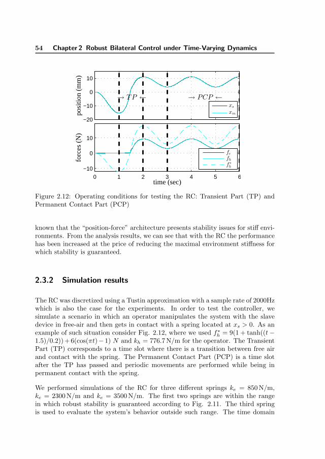
54 Chapter 2 Robust Bilateral Control under Time-Varying Dynamics
−20
−10
0
10po
sitio
n (m
m)
→ TP ← → PCP ←
xsxm
0 1 2 3 4 5 6
−10
0
10
forc
es (
N)
time (sec)
fefhf∗
h
Figure 2.12: Operating conditions for testing the RC: Transient Part (TP) andPermanent Contact Part (PCP)
known that the “position-force” architecture presents stability issues for stiff envi-ronments. From the analysis results, we can see that with the RC the performancehas been increased at the price of reducing the maximal environment stiffness forwhich stability is guaranteed.
2.3.2 Simulation results
The RC was discretized using a Tustin approximation with a sample rate of 2000Hzwhich is also the case for the experiments. In order to test the controller, wesimulate a scenario in which an operator manipulates the system with the slavedevice in free-air and then gets in contact with a spring located at xs > 0. As anexample of such situation consider Fig. 2.12, where we used f∗h = 9(1 + tanh((t−1.5)/0.2)) + 6(cos(πt)− 1) N and kh = 776.7 N/m for the operator. The TransientPart (TP) corresponds to a time slot where there is a transition between free airand contact with the spring. The Permanent Contact Part (PCP) is a time slotafter the TP has passed and periodic movements are performed while being inpermanent contact with the spring.
We performed simulations of the RC for three different springs ke = 850 N/m,ke = 2300 N/m and ke = 3500 N/m. The first two springs are within the rangein which robust stability is guaranteed according to Fig. 2.11. The third springis used to evaluate the system’s behavior outside such range. The time domain

2.3 Robust control applied to a 1-DoF academic setup 55
0
2
4
6
8
10
12ke = 850N/m
posi
tion
(mm
)
4 5 60
5
10
15
forc
e (N
)
time (sec)
ke = 2300N/m
4 5 6time (sec)
ke = 3500N/m
xsxm
4 5 6time (sec)
fefh
Figure 2.13: Time domain responses from simulations of interaction with differentsprings during the PCP.
signals of positions and forces for the PCP are presented in Fig. 2.13.
One can see that for all spring values, position and force tracking is achieved. Theposition tracking is slightly degraded for increasing values of environment stiffness.Such tendency of performance degradation was already observed in Fig. 2.11. Thesystem is still stable for ke = 3500 N/m though the robust analysis test performedin the previous section does not guarantee robust stability. We further analyzethe performance of the RC via force vs. position plots. Because such plots area good indication of the system’s performance for fixed environments, they werealso obtained for the controllers based on the P-P and P-F architectures wheninteracting with the soft spring with ke = 850 N/m.
The forces fh and fe are displayed against the positions xm and xs in Fig. 2.14.For illustrative purposes, the forces and positions plots are shifted such that all theplots at the environment side have the (0, 0) point in common. The slope of the fevs. xs plots represent the stiffness of environment and the slope of the fh vs. xmplots represent the stiffness being felt by the operator. For all test springs usingthe RC, the slopes of the plots of the operator and environment sides are similar,thus the operator feels a realistic spring in all cases and a high performance is

56 Chapter 2 Robust Bilateral Control under Time-Varying Dynamics
−1 0 1 2 3 4 5 6 7 8−1
0
1
2
3
4
5
6
7
8
9
10
kr ≈ 1300N/m
Force(N
)
Position (mm)
ke = 2300N/mke = 3500N/m
kr ≈ 1150N/m
ke = 850N/m
EnvironmentOperator RC
Operator P-P
Operator P-F
Figure 2.14: Force vs Position plots from simulations of interaction with differentsprings during the PCP. Controllers P-P and P-F are tested for ke = 850N/m.
indeed achieved. As already observed from the time domain plots, the performanceslightly decreases for increasing environment stiffness values. Next, Fig. 2.14 showsthat for soft environments, the P-P and P-F architectures have lower performancecompared to the RC. The reflected stiffness kr to the operator is bigger than theenvironment stiffness of ke = 850 N/m. The operator feels a stiffer environmentwith the classical architectures, being more noticeable for the P-P controller. Theseresults confirm the theoretical analysis previously performed.
Regarding the TP behavior, the corresponding time domain signals to the RC areshown in Fig. 2.15. Especially for ke = 850 N/m and ke = 2300 N/m, a smoothtransition is made despite the sudden change in environment stiffness, validatingthe robust performance properties of the proposed RC. For the third spring, whichis larger than ke with guaranteed performance, one can observe a small overshootat the transition instance and tracking performance worsens.
2.3.3 Experiments
In this section, we validate the promising simulation results with experimentson a physical setup. We test three springs with stiffness values ke≈ 850 N/m,ke≈ 2300 N/m and ke≈ 3500 N/m respectively. They were placed below the end-
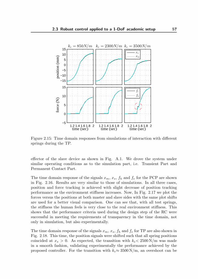
2.3 Robust control applied to a 1-DoF academic setup 57
−15
−10
−5
0
5
10
15ke = 850N/m
posi
tion
(mm
)
1.2 1.4 1.6 1.8 2−5
0
5
10
15
forc
e (N
)
time (sec)
ke = 2300N/m
1.2 1.4 1.6 1.8 2time (sec)
ke = 3500N/m
xs
xm
1.2 1.4 1.6 1.8 2time (sec)
fefh
Figure 2.15: Time domain responses from simulations of interaction with differentsprings during the TP.
effector of the slave device as shown in Fig. A.1. We drove the system undersimilar operating conditions as to the simulation part, i.e. Transient Part andPermanent Contact Part.
The time domain response of the signals xm, xs, fh and fe for the PCP are shownin Fig. 2.16. Results are very similar to those of simulations. In all three cases,position and force tracking is achieved with slight decrease of position trackingperformance as the environment stiffness increases. Now, In Fig. 2.17 we plot theforces versus the positions at both master and slave sides with the same plot shiftsare used for a better visual comparison. One can see that, with all test springs,the stiffness the human feels is very close to the real environment stiffness. Thisshows that the performance criteria used during the design step of the RC weresuccessful in meeting the requirements of transparency in the time domain, notonly in simulation, but also experimentally.
The time domain response of the signals xm, xs, fh and fe for TP are also shown inFig. 2.18. This time, the position signals were shifted such that all spring positionscoincided at xs > 0. As expected, the transition with ke< 2500 N/m was madein a smooth fashion, validating experimentally the performance achieved by theproposed controller. For the transition with ke≈ 3500 N/m, an overshoot can be

58 Chapter 2 Robust Bilateral Control under Time-Varying Dynamics
5
10
15
ke ≈ 850N/m
posi
tion
(mm
)
36 37 38
5
10
15
forc
e (N
)
time (sec)
ke ≈ 2300N/m
28 28.5 29time (sec)
ke ≈ 3500N/m
xsxm
29 29.5 30time (sec)
fefh
Figure 2.16: Time domain responses from experiments of interaction with differentsprings during the PCP.
0 2 4 6 8 10−1
0
1
2
3
4
5
6
7
8
9
ke ≈ 850N/m
Force(N
)
Position (mm)
ke ≈ 2300N/mke ≈ 3500N/m
Environment
Operator
Figure 2.17: Force vs Position plot from experiments of interactions with differentsprings during the PCP.

2.3 Robust control applied to a 1-DoF academic setup 59
−20
−10
0
10
ke ≈ 850N/m
posi
tion
(mm
)
53 53.5 54−5
0
5
10
15
forc
e (N
)
time (sec)
ke ≈ 2300N/m
54 54.5 55time (sec)
ke ≈ 3500N/m
xsxm
46 46.5 47time (sec)
fefh
Figure 2.18: Time domain responses from experiments during the TP of a transi-tion from free air to different springs at xs > 0
observed especially in the force signals. According to our robust performance anal-ysis from Fig. 2.11 stability is not guaranteed. In practice, we only experienced theovershoot but we could not destabilize the system. However, such overshoot candegrade the subjective haptic perception of the environment. Though the analysiscan introduce conservatism, it still ensures a safe and high performance opera-tion of the system under realistic conditions in which the human an environmentdynamics vary with time.
Finally, the TP time slot is further analyzed and the corresponding power spectraldensity plots are shown in Fig. 2.19 . For all cases, the system presented positiontracking up to 10 Hz and force tracking up to 4 Hz for the time-varying stiffness.Thus, practically high-performance is achieved up to 4 Hz. One can see that forthe third stiffness the overshoot can be also noticed in frequency-domain by anincrease of the power concentration of the environment forces between [4,10] Hz,which might not be safe for the environment, for instance when the environmentis, say a soft tissue. Therefore, it is validated that Fig. 2.11 can give a goodindication for the safe region of operation of the bilateral system, which showsthat the model and the assumptions we made are sufficiently realistic.
As final remarks, we have assumed that the human arm-hand stiffness can vary in-
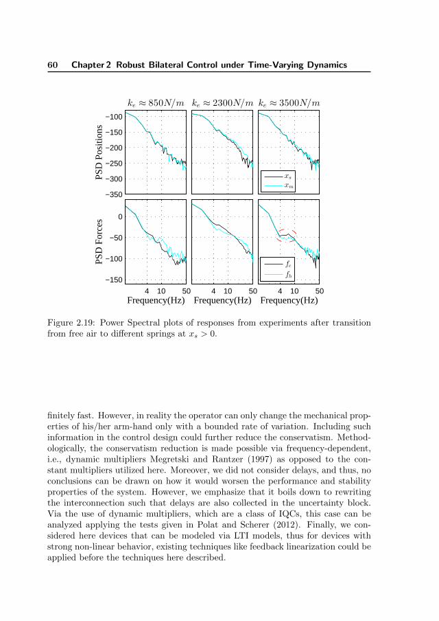
60 Chapter 2 Robust Bilateral Control under Time-Varying Dynamics
−350
−300
−250
−200
−150
−100
ke ≈ 850N/mPS
D P
ositi
ons
4 10 50
−150
−100
−50
0
Frequency(Hz)
PSD
For
ces
ke ≈ 2300N/m
4 10 50Frequency(Hz)
ke ≈ 3500N/m
xsxm
4 10 50Frequency(Hz)
fefh
Figure 2.19: Power Spectral plots of responses from experiments after transitionfrom free air to different springs at xs > 0.
finitely fast. However, in reality the operator can only change the mechanical prop-erties of his/her arm-hand only with a bounded rate of variation. Including suchinformation in the control design could further reduce the conservatism. Method-ologically, the conservatism reduction is made possible via frequency-dependent,i.e., dynamic multipliers Megretski and Rantzer (1997) as opposed to the con-stant multipliers utilized here. Moreover, we did not consider delays, and thus, noconclusions can be drawn on how it would worsen the performance and stabilityproperties of the system. However, we emphasize that it boils down to rewritingthe interconnection such that delays are also collected in the uncertainty block.Via the use of dynamic multipliers, which are a class of IQCs, this case can beanalyzed applying the tests given in Polat and Scherer (2012). Finally, we con-sidered here devices that can be modeled via LTI models, thus for devices withstrong non-linear behavior, existing techniques like feedback linearization could beapplied before the techniques here described.

2.4 Conclusions 61
2.4 Conclusions
In this chapter, we have presented a systematic approach towards control designfor bilateral teleoperation. Such approach uses a parametric model of a bilateralteleoperation system, this allowed us to handle the uncertain parameters of thebilateral system systematically. Operator and environment with bounded andtime-varying stiffness were considered. The experimental results demonstratedthat such uncertainty description allowed to obtain high performance and stabilitysimultaneously in the range of soft environments, not only for continued contactwith the environment, but also for sudden changes in it. Moreover, the analysis,simulation and experimental results of the controlled system were consistent witheach other, showing that the assumptions we made during modeling and synthesiswere appropriate, thus demonstrating the potential of the design methodology herepresented.
In the next chapter, dependency on the environment properties are included duringcontrol design, allowing for different controller for soft and hard environments.

62
63
Chapter 3
Switching Robust Control forBilateral Teleoperation
WHEN the environment of the teleoperation system varies within alarge range, a single controller might not be sufficient to achieve
both stability and high performance. In this chapter we propose the syn-thesis of a switching robust controller that allows to design multiple robustcontrollers suitable for different ranges of environment stiffness, so that anoverall better performance is achieved. The controllers are scheduled usingan estimate of the environment stiffness. During the design we accountfor smooth switching among controllers and for the fact that environmentestimators will have limited accuracy and uncertainty. We present syn-thesis, simulation and experimental results of the proposed approach, thusshowing the effectiveness of the method to improve the robust performanceof the teleoperated system.
3.1 Introduction
Teleoperation systems can provide a feeling of tele-presence using force feedbackwhile an operator manipulates a remote environment by means of a master and aslave device. It is desirable that the system has high performance, e.g. the opera-tor feels as if he/she is manipulating the environment directly, in a stable fashion.
This chapter is based on the following manuscript: Lopez Martınez, C. A., Molengraft, R.v. d., and Steinbuch, M. (2014c). Switching robust control for bilateral teleoperation. Underreview for journal publication

64 Chapter 3 Switching Robust Control for Bilateral Teleoperation
However, there is an inherent trade-off between (robust) stability and performance,see, e.g., Hannaford (1989); Lawrence (1993b), and it is a challenging problem todesign controllers that meet an appropriate balance, see, e.g., Hokayem and Spong(2006), Passenberg et al. (2010). Control design tools based on Passivity theory,see, e.g., Niemeyer and Slotine (1991), Ryu (2007), have been widely used. Theymainly focus on stability but the stability/performance trade-off is not taken intoaccount systematically. More recent works by, e.g. Kim et al. (2013), Willaertet al. (2014) consider performance in the design, but either neglect the fact thatboth operator and environment dynamics are inherently time-varying, or the ap-plicability is limited to master and slave devices with identical mass-damper-springdynamics.
Additionally, in many applications environment parameters such as mass, dampingand stiffness are bounded. In Chapter 2, we included this boundedness into thecontrol design process to balance performance and stability. We also experimen-tally validated the design of a robust Linear Time Invariant (LTI) controller, whichyields a high performance for time-varying environment stiffness in the range ofthose encountered in soft tissues in applications such as minimally invasive surgery,needle insertion, etc. However, in the same sort of applications there are other tis-sues with larger stiffness coefficients, for example up to around 7000N/m for theribcage (Bankman et al. (1990)) and there might even be rigid contacts, e.g. inthe collision of two robotic arms. Therefore, it is desirable to increase the range inwhich performance and stability is achieved in order to get closer to the require-ments of real-life surgical conditions.
On the other hand, there is no guarantee that a single LTI controller exists that en-sures both performance and stability for a large range of time-varying environmentstiffness values. To cover a large region of environment stiffness, one can add flex-ibility in the control design, for instance by means of estimating the environmentstiffness and use such estimation to design a controller that adapts accordingly.Some works, e.g. by Willaert et al. (2010), Cho et al. (2013), design controllersthat depends on the estimate of the environment stiffness, however either they donot guarantee robust performance, or the achieved operating range is limited tolow environment stiffness. Moreover, such works rely on accurate, unbiased, lownoise and/or fast convergence of the estimated environment stiffness, requirementswhich in practice are difficult to meet simultaneously.
Another approach to address performance and stability, when the environmentstiffness varies in a wide range, is the use of switching control. Some existingswitching control methods suggest to switch between different operating points ofthe overall system, see, e.g., Liberzon (2003), Leith and Leithead (2000), thoughsystems with uncertainty are not considered and/or smooth switching is not guar-anteed. Multiple model adaptive control, which is also a switching based method,

3.2 Switching robust control approach 65
has been used in teleoperation in Shahdi and Sirouspour (2005), however uncer-tainty in the operator is not included and there is no smooth switching betweencontrollers.
We propose the use of a switching robust controller that accounts for uncertaintyin the operator and environment dynamics as well as uncertainty and noise inthe estimation of the environment stiffness ke that is used for control schedul-ing. We use operator and environment models such that the uncertainty ∆ in thebilateral teleoperation system is defined by the operator and environment stiff-ness parameters. The human operator’s model structure is based on an operator’shand measurements. The proposed multi-controller structure consists of Nc LTIrobust controllers, in which the ith controller has robust performance in an un-certainty region ∆i, such that all regions combined cover the uncertainty set ∆.Moreover, such controllers are designed to share a common quadratic Lyapunovfunction, which ensures stable and smooth switching between them. Additionally,to be robust to uncertainty and noise in the estimated parameter that allows thescheduling of the robust controllers, we define a minimum overlapping between theregions ∆i.
In this thesis it is the first time that experiments are presented using switchingrobust control in teleoperation, such that robust performance is guaranteed undertime-varying uncertainty in the operator, the environment, and the estimation ofthe scheduling parameter ke. The synthesis, simulations and experiments demon-strate the potential of the proposed method to improve the robust performance inteleoperation systems.
In Section 3.2 we describe the system’s modelling and the framework for controldesign of the proposed switching robust controller for teleoperation systems. Syn-thesis, Simulations and experimental results are presented and discussed in Section3.3. Finally, in Section 3.4 the conclusions are presented.
3.2 Switching robust control approach
3.2.1 LFR model of a teleoperation system
Similarly as in Chapter 2, we make use of a Linear Fractional Representation(LFR) of the bilateral teleoperation system. Deriving a LFR of a system amountsto isolating the uncertain parameters such that an interconnection structure asdepicted in Fig. 3.1 is obtained. Let δi = [δi, δi], i = 1, . . . , np be families ofbounded parametric uncertainties with possibly different lower and upper bounds.

66 Chapter 3 Switching Robust Control for Bilateral Teleoperation
∆(δ)
Gnomin out
Figure 3.1: Linear Fractional Representation of a System.
Let δi(t) ∈ δi, i = 1, . . . , np be parametric uncertainties and define the vector δ asthe vector of all np parametric uncertainties, that is, δ = col(δ1, . . . , δnp) ∈ Rnp .∆(δ) is the block diagonal mapping that acts on δ, i.e. ∆(δ) = diag(δ1, . . . , δnp
).q and p are the signals interfacing with the uncertainty block in the sense thatp = ∆(δ)q. In particular, at any time instant t this means that p(t) = ∆(δ(t))q(t)is an ordinary matrix multiplication. To derive the LFR model of the teleoperationsystem, the uncertainty parameters δ are defined and then isolated and collectedinto the uncertainty block ∆(δ). To this end, we first define the models of thedifferent components of a teleoperation system. We apply our methods on a sys-tem using the particular mass-damper-spring models for master and slave devices,which interact with the operator and environment respectively as depicted in Fig.3.2, where mm > 0, bm ≥ 0, km ≥ 0 are the fixed parameters of the master device;ms > 0, bs ≥ 0, ks ≥ 0 are the fixed parameters of the slave device; fm, fs are theactuation forces to the master and slave devices respectively; fh, fe represent thetotal force exerted by the operator and environment respectively; and xm, xs arethe positions of the master and slave devices respectively. By definition they alsorepresent the positions of the operator and environment respectively.
Operator
1
mms2 + bms+ km
fm
fh
xm
(a)
Environment
1
mss2 + bss+ ks
fs
fe
xs
−
(b)
Figure 3.2: Diagram of (a) operator/master device and (b) environment/slavedevice.
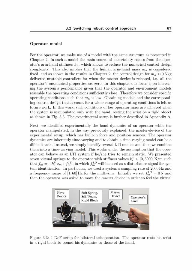
3.2 Switching robust control approach 67
Operator model
For the operator, we make use of a model with the same structure as presented inChapter 2. In such a model the main source of uncertainty comes from the oper-ator’s arm-hand stiffness kh, which allows to reduce the numerical control designcomplexity. This also implies that the human arm-hand mass mh is consideredfixed, and as shown in the results in Chapter 2, the control design for mh ≈ 0.5 kgdelivered unstable controllers for when the master device is released, i.e. all theoperator’s mechanical properties are zero. In this chapter our focus is on increas-ing the system’s performance given that the operator and environment modelsresemble the operating conditions sufficiently close. Therefore we consider specificoperating conditions such that mh is low. Obtaining models and the correspond-ing control design that account for a wider range of operating conditions is left asfuture work. In this work, such conditions of low operator mass are achieved whenthe system is manipulated only with the hand, resting the wrist on a rigid objectas shown in Fig. 3.3. The experimental setup is further described in Appendix A.
Next, we identified experimentally the hand dynamics of an operator while theoperator manipulated, in the way previously explained, the master-device of theexperimental setup, which has built-in force and position sensors. The operatordynamics are inherently time-varying and to obtain a time-varying model can be adifficult task. Instead, we simply identify several LTI models and then we combinethem into a time-varying model. This works under the assumption that the oper-ator can behave as an LTI system if he/she tries to remain static. We presentedseven virtual springs to the operator with stiffness values kVe ∈ [0, 5000] N/m suchthat fm = −kVe xm+f IDm , in which f IDm will be used as a disturbance signal for sys-tem identification. In particular, we used a system’s sampling rate of 2000 Hz anda frequency range of [1, 60] Hz for the multi-sine. Initially we set f IDm = 0 N andthen the operator was asked to move the master device in order to feel the virtual
Soft Spring,Stiff Foam,Rigid Block
SlaveDevice
MasterDevice Operator’s
hand
Figure 3.3: 1-DoF setup for bilateral teleoperation. The operator rests his wristin a rigid block to bound his dynamics to those of the hand.
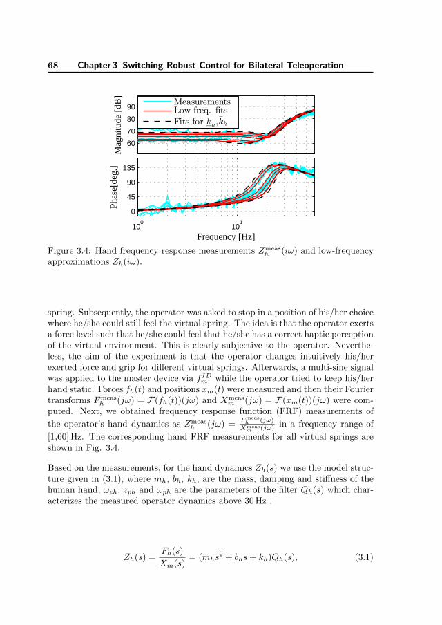
68 Chapter 3 Switching Robust Control for Bilateral Teleoperation
60
70
80
90
Mag
nitu
de [
dB]
100
101
0
45
90
135
Frequency [Hz]
Phas
e[de
g.]
MeasurementsLow freq. fits
Fits for kh,kh
Figure 3.4: Hand frequency response measurements Zmeash (iω) and low-frequency
approximations Zh(iω).
spring. Subsequently, the operator was asked to stop in a position of his/her choicewhere he/she could still feel the virtual spring. The idea is that the operator exertsa force level such that he/she could feel that he/she has a correct haptic perceptionof the virtual environment. This is clearly subjective to the operator. Neverthe-less, the aim of the experiment is that the operator changes intuitively his/herexerted force and grip for different virtual springs. Afterwards, a multi-sine signalwas applied to the master device via f IDm while the operator tried to keep his/herhand static. Forces fh(t) and positions xm(t) were measured and then their Fouriertransforms Fmeas
h (jω) = F(fh(t))(jω) and Xmeasm (jω) = F(xm(t))(jω) were com-
puted. Next, we obtained frequency response function (FRF) measurements of
the operator’s hand dynamics as Zmeash (jω) =
Fmeash (jω)
Xmeasm (jω) in a frequency range of
[1,60] Hz. The corresponding hand FRF measurements for all virtual springs areshown in Fig. 3.4.
Based on the measurements, for the hand dynamics Zh(s) we use the model struc-ture given in (3.1), where mh, bh, kh, are the mass, damping and stiffness of thehuman hand, ωzh, zph and ωph are the parameters of the filter Qh(s) which char-acterizes the measured operator dynamics above 30 Hz .
Zh(s) =Fh(s)
Xm(s)= (mhs
2 + bhs+ kh)Qh(s), (3.1)

3.2 Switching robust control approach 69
1s
1s
1mm
xmxmxm
mh
bh
kh
bm
km
f∗h
fh
fm
Master Device
Operator
−
−Qh(s)
∆h
Figure 3.5: Block diagram representation of the operator/master device pair.
where
Qh(s) =
s
ωzh+ 1
s2
ω2ph
+ 2zphs
ωph+ 1
.
Then, we optimized the variables mh, bh, kh, ωzh, zph and ωph to fit each measure-ment to the model minimizing the cost function WZh
(iω) = ‖(Zh(iω)−Zmeash (iω))/
|Zmeash (iω)|‖2 for ω ∈ 2π[1, 60] rad/s. The optimization is done using a constrained
nonlinear optimization method provided by the command fmincon in Matlabr.In practice the optimization problem has several local minima, thus initial con-ditions and interval constraints must be provided to the solver. Those initialconditions and their respective constraints are estimated based on the measure-ments and are adjusted until a satisfactory match between Zh(iω) and Zmeas
h (iω) isobtained. The resulting parameters were found to be within the following ranges;mh ∈ [0.112, 0.134] kg, bh ∈ [5.88, 8.94] N s/m, kh ∈ [1257, 2501] N/m, ωzh ∈[69.5, 102.5] rad/s, zph ∈ [0.54, 0.70] and ωph ∈ [184.0, 239.8] rad/s. To reducecomplexity of the model and control design, we have used a low-frequency approxi-mation by allowing variation in kh only and fixing all other parameters to their cen-tered values in the corresponding intervals, thus mh = 0.123 kg, bh = 7.41 N s/m,ωzh = 86 rad/s, zph = 0.62 and ωph = 211.9 rad/s. The corresponding fitted mod-els are depicted in Fig. 3.4. Finally, to include possible extra variation in kh, weenlarge the range of values of kh by 20%, and we use kh ∈ [1131.3, 2751.1] N/m.The resulting Zh(s) fitted models for kh and kh are depicted with dashed linesin Fig. 3.4. One can see that the approximation fits well for low frequencies and,moreover, allows to reduce the number of uncertain parameters in the operator

70 Chapter 3 Switching Robust Control for Bilateral Teleoperation
model. Because only kh is considered uncertain, using the model proposed here forcontrol design has implications. Mainly, the system’s performance could decreasefor users with dynamic properties that differ largely from those considered here.It is possible to extend the number of uncertainty parameters in the operator’smodel at the cost of increasing the numerical complexity of the synthesis proce-dure. The operator identification was performed for a single operator. From thearm-hand models presented here and in Chapter 2, we can already conclude thatthe structure of Eq. 3.1 covers sufficiently well the dynamics of different arm-handconfigurations, i.e. different arm-hand poses that result in the use of differentgroups of muscles. This is an indication that the operator’s model-structure pre-sented here could be valid for other users as well. Regarding the range of variationof the operator’s model-parameters, it is clear that different arm-hand configura-tions result in different ranges of variation of parameters. This can be seen if wecompare the parameters found here with those in Chapter 2. Furthermore, theparameters are expected to vary among different users. Nevertheless, less variationis expected if the arm-hand pose during experiments is similar among users. How-ever, more subjects are needed to evaluate whether the structure of the operator’smodel and the proposed low frequency approximation are still valid.
Though the identification was performed via LTI techniques, in what follows below,we assume that during operation kh is time-varying in the sense that kh(t) ∈[kh, kh] for all t > 0.
Finally, combining the master device and operator models, we arrive at the modeldiagram for the operator/master device depicted in Fig. 3.5, where f∗h is the activeforce generated by the operator and ∆h = kh defines the time-varying, boundedand uncertain parameter of the human hand dynamics model.
Environment model
Next, we consider environments with mass-damper-spring dynamics:
fe = f∗e + (mexs + bexs + kexs),
which model a significant class of applications of interest. Here, me, be and keare the non-negative mass, damping and stiffness coefficients of the environmentrespectively, and f∗e is the active force from the environment, if present. We focuson the environment stiffness ke as the main cause of the dynamic variation, henceme and be are assumed fixed and ke is assumed to be bounded (though withina wide range), and in addition time-varying. This choice is suitable for applica-tions in which the effect of ke on fe is dominant, e.g. in stiffness discriminationtasks like those in surgery. For other environment types the uncertainty struc-ture and parameters can be redefined. One should keep in mind that because of
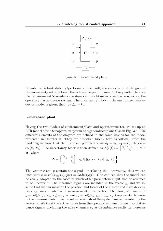
3.2 Switching robust control approach 71
G
∆(δ)
Kc
w z
p
u
q
y
Figure 3.6: Generalized plant.
the intrinsic robust stability/performance trade-off, it is expected that the greaterthe uncertainty set, the lower the achievable performance. Subsequently, the cou-pled environment/slave-device system can be obtain in a similar way as for theoperator/master-device system. The uncertainty block in the environment/slave-device model is given, then, by ∆e = ke.
Generalized plant
Having the two models of environment/slave and operator/master, we set up anLFR model of the teleoperation system as a generalized plant G as in Fig. 3.6. Thedifferent elements of the diagram are defined in the same way as for the modelpresented in Chapter 2. They are described briefly here as follows: From themodeling we have that the uncertain parameters are δ1 = kh, δ2 = ke, thus δ =
col(kh, ke). The uncertainty block is then defined as ∆(δ(t)) =[kh(t) 0
0 ke(t)
], ∆ ∈
∆, where
∆ =
{[kh 00 ke
]: kh ∈ [kh, kh], ke ∈ [ke, ke]
}.
The vector q and p contain the signals interfacing the uncertainty, thus we caninfer that q = col(xm, xs), p(t) = ∆(δ(t))q(t). One can see that the model canbe easily adapted to the cases in which other parameters might also be assumedto be uncertain. The measured signals are included in the vector y, and we as-sume that we can measure the position and forces of the master and slave devices,possibly contaminated with measurement noise vector. Therefore, we have thaty = col(fh, fe, xm, xs)+yn, where yn = col(fhn, fen, xmn, xsn) represents the noisein the measurements. The disturbance signals of the system are represented by thevector w. We treat the active forces from the operator and environment as distur-bance signals. Including the noise channels yn as disturbances explicitly increases

72 Chapter 3 Switching Robust Control for Bilateral Teleoperation
the robustness properties that would help to obtain a controller more suitable forthe actual implementation. Thus, we define w = col(f∗h , f
∗e , fhn, fen, xmn, xsn).
Additionally, the actuation signal vector u contains the forces actuated from themotors of the master and the slave devices. Thus, u = col(fm, fs). The perfor-mance vector z is defined as z = col(fh− fe, xm−xs, fm, fs). Via the component,fh − fe, we enforce that the human operator should feel the same force appliedby the environment. The second component, xm − xs, is the position error to ob-tain tracking between master and slave. The actuation variables are also includedas channels to be penalized to avoid controllers with high gains. G is the LTImodel that contains all the fixed model dynamics of the different components ofthe bilateral teleoperation system: the master device, the slave device, the fixedoperator dynamics and the fixed environment dynamics if present. Finally, Kc isthe to-be-designed controller that maps the measured signals y to the actuationsignals u.
The control design problem is then to find a controller Kc that achieves robuststability and robust performance for all ∆ ∈ ∆. At this point we still need todefine what structure the controller Kc will have, which will be the subject of thenext section.
3.2.2 Switching robust control design using a commonquadratic Lyapunov function
In Chapter 2, using Linear Matrix Inequalities (LMI’s) (Scherer and Weiland(2010)), we synthesized a single LTI robust controller with robust performancefor bounded environment stiffness ke in the range of low stiffness environments.Our research focus is on obtaining high performance teleoperated systems for awider range of environment stiffness ke ∈ [ke, ke], covering not only soft stiffnessenvironments. As it will be shown later, the achievable performance of controllersdesigned with the methodology presented in Chapter 2 degrades considerably asthe maximal environment stiffness ke is increased. From a control point of view,one of the reasons for this performance degradation is the lack of flexibility of thecontroller to adapt to large changes in the uncertainty parameters of the system.Therefore, in this chapter we present control architecture in which we increase theflexibility of the controller architecture so we can achieve a better performanceindex and therefore reduce the performance degradation for large ranges of ke.
We propose a switching robust control architecture. The main idea consists ofscheduling different robust controllers according to the estimate ke of the actualvalue of ke. Thus, we design a specific number Nc of LTI controllers, in whichthe ith controller has an uncertainty set ∆i of robust performance, such that all

3.2 Switching robust control approach 73
regions combined form a larger set such that ∆ ⊆ ∆1 ∪ . . . ∪ ∆Nc, where ∆
describes the uncertainty region of the system.
To describe the partition, let δ(i)j = [δ(i)j , δ(i)j ], i = 1, . . . , Nc; j = 1, . . . , np befamilies of bounded parametric uncertainties. Let δ(i)j(t) ∈ δ(i)j , i = 1, . . . , Nc;j = 1, . . . , np be parametric uncertainties and define the vectors δ(i) = col(δ(i)1, . . . ,δ(i)np
) ∈ Rnp , i = 1, . . . , Nc. ∆i(δ(i)), i = 1, . . . , Nc are the block diagonal map-pings that acts on δ(i), i.e. ∆i(δ(i)) = diag(δ(i)1, . . . , δ(i)np
), i = 1, . . . , Nc. Then,each subregion ∆i is described by ∆i ∈∆i, where the class ∆i is defined as
∆i ={
diag(δ(i)1, . . . , δ(i)np) : δ(i)1 ∈ [δ(i)1, δ(i)1], . . . , δ(i)np
∈ [δ(i)np, δ(i)np
]}
for i = 1, . . . , Nc, that ∆ ⊆∆1∪ . . .∪∆Nc . In our specific case np = 2. Thereforeeach regions ∆i, i = 1, . . . , Nc is a ‘rectangle’ in the kh − ke plane. The specificdistribution of ∆i, i = 1, . . . , Nc will be given in Section 3.2.3.
Augmented plant model for control design
Before describing the control synthesis method, we need to augment the modelshown in Fig. 3.6 in order to incorporate the uncertainty partitions ∆i, i = 1, . . . , Ncand a more suitable form that is usable for control design. To this end, considerthe model diagram presented in Fig. 3.7 in which we have augmented and parti-tioned the model in Fig. 3.6 in Nc augmented generalized plants Gi. The differentcomponents of the augmented model are described as follows:
� V and W are weighting filters described with stable LTI systems. They allowto shape in frequency domain the desired system performance. These filterswill be defined in detail in Section 3.2.5. Meanwhile they are assumed to beknown.
� w and z are weighted copies of w and z via predefined filters V and Wrespectively. That is w = V w and z = Wz.
� δ(i), i = 1, . . . , Nc. are the vectors δ(i) = col(δ(i)1, . . . , δ(i)np) of the trans-
formed uncertain parameters δ(i)j ∈ δ(i)j such that δ(i)j = [δ(i)j , δ(i)j ] and
0 ∈ δ(i)j for i = 1, . . . , Nc and j = 1, . . . , np. The main idea is that the
intervals δ(i)j are mapped one to one to the intervals δ(i)j . The specific
transformations from parameters δ(i)j to δ(i)j will be given in Section 3.2.3.Meanwhile they are assumed to be known.
� ∆i(δ(i)), i = 1, . . . , Nc is the block diagonal concatenation of the parameters

74 Chapter 3 Switching Robust Control for Bilateral Teleoperation
G
T∆i
∆i(δ(i))
r
W
Kci
Vw zw z
u y
qp
pi qi
Gi
Figure 3.7: Set of generalized plants with weighting filters, uncertainty transfor-mation and scaling. The dashed block in the upper part equals ∆i(δ) providedr = 1.
in ˜δ(i).
∆i(δi(t)) = diag(δ(i)1, . . . , δ(i)np), ∆i ∈ ∆i,
where
∆i ={
diag(δ(i)1, . . . , δ(i)np) : δ(i)1 ∈ [δ(i)1, δ(i)1], . . . , δ(i)np
∈ [δ(i)np, δ(i)np
]}
for i = 1, . . . , Nc.
� The vector q and p contain the signals interfacing the new uncertainty block∆. Thus p(t) = ∆(δ(t))q(t).
� r ∈ [0, 1]: is a scaling factor that allows to scale down the uncertainty blocks∆i. This allows to perform an iterative process during the control designin which one starts with the nominal case r = 0, i.e. no uncertainty, andfinalizes with an unscaled uncertainty set for r = 1. We will refer to anominal plant if r = 0. If r = 1 we have that ∆i(δi) equals the dashed blockin the upper part of Fig. 3.7.
� T∆i: R2np×2np , i = 1, . . . , Nc are constant matrices such that :
(qip
)=
(r 00 1
)T∆i
(piq
), i = 1, . . . , Nc
T∆iis used to map one to one the uncertain parameter set ∆i to the trans-
formed uncertain parameter set ∆i. The transformations T∆iallows to
3.2 Switching robust control approach 75
obtain a nominal values of ∆i(δNom(i) ) ∈ ∆i for r = 0. The specific transfor-
mations from matrices T∆i,i=1,...,Ncwill be given in Section 3.2.3. Meanwhile
they are assumed to be known.
� Kci, i = 1, . . . , Nc are then the LTI controllers Kci(s) = Cci(Is−Aci)−1Bci+Dci, which we will identify with its state space description by writing
Kci(s) =
[Aci BciCci Dci
],
One can derive a model of the generalized plant Gi for i = 1, . . . , Nc. We denoteits state space representation by the following equation:
xqizy
=
Ai B(i)1 B(i)2 BirC(i)1 rD(i)1 rD(i)12 rE(i)1
C(i)2 D(i)21 D(i)2 E(i)2
Ci F(i)1 F(i)2 0
xpiwu
, i = 1, . . . , Nc
Uncertainty and performance description
Similarly as in Chapter 2, we will use a specific class of Integral Quadratic Con-straints (IQCs) (see Megretski and Rantzer (1997)) to model uncertainties ∆i ∈∆i. Then consider Pi as sets of symmetric matrices Pi ∈ R2np×2np that satisfythe following IQC
∫ T0
0
(∆i(δi)qi(t)
qi(t)
)TPi
(∆i(δi)qi(t)
qi(t)
)dt ≥ 0 (3.2)
for all q ∈ L2[0, T0], T0 ∈ R+, ∆i ∈ ∆i and i = 1, . . . , Nc.
The matrix Pi for a specific i is a so called multiplier. It allows to describemathematical properties of the uncertainty block ∆i. The set Pi needs to befurther classified in order to describe specific type of uncertainties. Because theclass ∆i is convex, it can be expressed as a convex combination of generatorsδj(i), j = 1, . . . , 2np . Then, as shown in Chapter 2, we can describe ∆i by means
of classifying the sets Pi by the symmetric matrices Pi that satisfy the followingfinite number of inequalities
(I0
)TPi
(I0
)� 0 (3.3)
(∆i(δ
j(i))
I
)TP
(∆i(δ
j(i))
I
)� 0, i = 1, . . . , Nc j = 1, . . . , 2np (3.4)

76 Chapter 3 Switching Robust Control for Bilateral Teleoperation
In fact, (3.3) and (3.4) imply also (3.2), see Sections 1.3 and 2.2.2. In thiscase, matrices Pi, i = 1, .., Nc are then constant full block multipliers describingbounded and time-varying real parametric uncertainties. Also notice that imposingstructure and dynamics in the matrices Pi, other types of uncertainty can bedescribed as shown in Polat and Scherer (2012), which can be exploited in futureworks. Once we characterize the uncertain sets ∆i by Pi, we will describe theperformance criterion used here.
We have chosen the performance criterion based upon the L2 gain of the mappingfrom disturbance channels w to the performance channels z as is customary inmodel-based H∞ control, e.g., see Skogestad and Postlethwaite (2005). The L2
gain from w to z can be expressed as:
sup06=w∈L2
||z||2||w||2
< γ, (3.5)
in which γ can be interpreted as a worst-case gain from the disturbances w to theperformance signals z. Therefore, instantaneous responses that can be felt by theoperator have a direct effect on the performance criterion. This makes the L2 gaina suitable performance criterion for teleoperation systems. The L2 gain can beexpressed in a standard form as a quadratic performance criterion:
∫ ∞
0
(w(t)z(t)
)TPp
(w(t)z(t)
)dt < 0 forall 0 6= w ∈ L2, (3.6)
with
Pp =
(−γ2I 0
0 I
)
The standard form to describe performance in Eq. (3.6) allows the use of otherquadratic performance criteria via Pp, see,e.g., Section 1.3 and Scherer and Weiland(2000). To keep the generality of the theory used here, we will use the symbol Ppto describe our specific performance criterion.
We proceed with the LMI-based switching robust controller design such that theclosed loop is robustly stable and satisfies the performance specifications. Therobust control synthesis concepts are adapted from Scherer and Weiland (2010).
Switching robust control synthesis using a common Lyapunov function
First, we describe a general framework to design switching robust controllers, thenin Section 3.2.3 we provide a more specific framework of the control design appliedto the bilateral teleoperation problem.
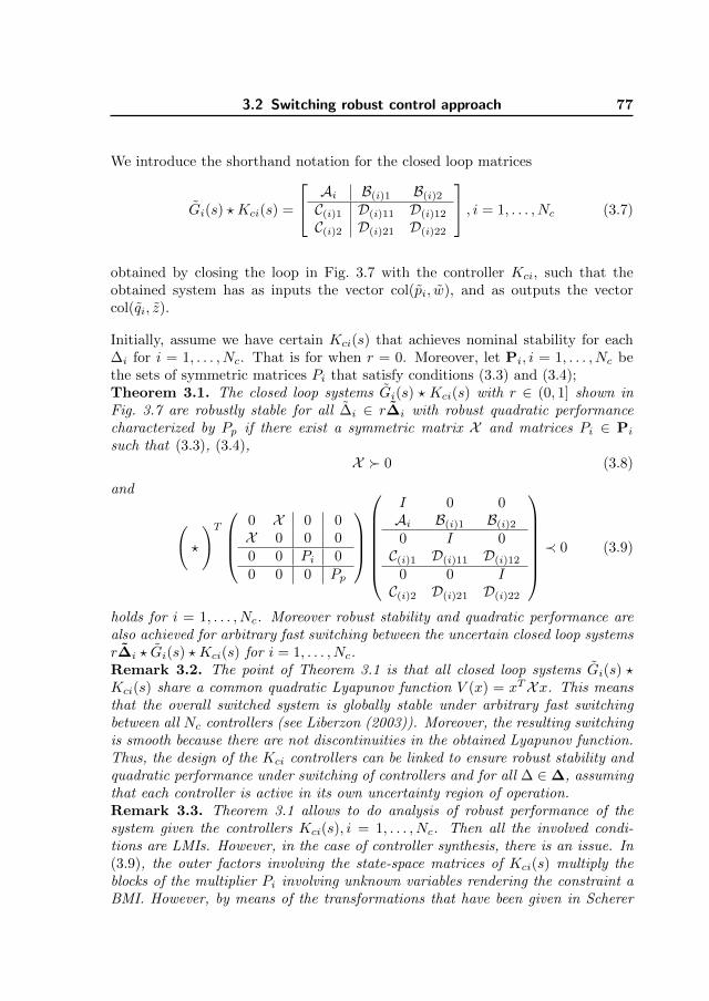
3.2 Switching robust control approach 77
We introduce the shorthand notation for the closed loop matrices
Gi(s) ? Kci(s) =
Ai B(i)1 B(i)2
C(i)1 D(i)11 D(i)12
C(i)2 D(i)21 D(i)22
, i = 1, . . . , Nc (3.7)
obtained by closing the loop in Fig. 3.7 with the controller Kci, such that theobtained system has as inputs the vector col(pi, w), and as outputs the vectorcol(qi, z).
Initially, assume we have certain Kci(s) that achieves nominal stability for each∆i for i = 1, . . . , Nc. That is for when r = 0. Moreover, let Pi, i = 1, . . . , Nc bethe sets of symmetric matrices Pi that satisfy conditions (3.3) and (3.4);Theorem 3.1. The closed loop systems Gi(s) ? Kci(s) with r ∈ (0, 1] shown inFig. 3.7 are robustly stable for all ∆i ∈ r∆i with robust quadratic performancecharacterized by Pp if there exist a symmetric matrix X and matrices Pi ∈ Pi
such that (3.3), (3.4),X � 0 (3.8)
and
(?
)T
0 X 0 0X 0 0 00 0 Pi 00 0 0 Pp
I 0 0Ai B(i)1 B(i)2
0 I 0C(i)1 D(i)11 D(i)12
0 0 IC(i)2 D(i)21 D(i)22
≺ 0 (3.9)
holds for i = 1, . . . , Nc. Moreover robust stability and quadratic performance arealso achieved for arbitrary fast switching between the uncertain closed loop systemsr∆i ? Gi(s) ? Kci(s) for i = 1, . . . , Nc.Remark 3.2. The point of Theorem 3.1 is that all closed loop systems Gi(s) ?Kci(s) share a common quadratic Lyapunov function V (x) = xTXx. This meansthat the overall switched system is globally stable under arbitrary fast switchingbetween all Nc controllers (see Liberzon (2003)). Moreover, the resulting switchingis smooth because there are not discontinuities in the obtained Lyapunov function.Thus, the design of the Kci controllers can be linked to ensure robust stability andquadratic performance under switching of controllers and for all ∆ ∈∆, assumingthat each controller is active in its own uncertainty region of operation.Remark 3.3. Theorem 3.1 allows to do analysis of robust performance of thesystem given the controllers Kci(s), i = 1, . . . , Nc. Then all the involved condi-tions are LMIs. However, in the case of controller synthesis, there is an issue. In(3.9), the outer factors involving the state-space matrices of Kci(s) multiply theblocks of the multiplier Pi involving unknown variables rendering the constraint aBMI. However, by means of the transformations that have been given in Scherer
78 Chapter 3 Switching Robust Control for Bilateral Teleoperation
and Weiland (2010); Masubuchi et al. (1998); Scherer. et al. (1997), it is possi-ble to make (3.9) an LMI when either Pi or (Aci, Bci, Cci, Dci) are fixed. More-over, (Aci, Bci, Cci, Dci) matrices also multiply each other, hence a linearization isneeded. Fortunately, this can be avoided with a Schur complement argument. InChapter 2 it is shown how to perform such linearization for one controller. Thisprocedure can be expanded to the multi-controller case in a straightforward way.
Initially, we have neither a controller nor a multiplier by which the constraints aresatisfied. Hence one typically starts with the nominal system Gnom = 0piqi?Gi, i =1, . . . , Nc (which is an upper LFT and equivalent to removing the uncertainty chan-nels). Then we design a nominally stabilizing controllers Kci(s), i = 1, . . . , Nc de-noted by Kcnom with certain performance level, utilizing equations in Theorem 3.1after removing the columns and rows corresponding to the uncertainty channels.As mentioned in remark 3.3, extra transformations are needed to arrive to LMI’sthat allow to design the controller parameters, mainly two steps are needed, firsta congruence transformation is used to arrive to transformed parameters and sub-sequently a linearisation lemma is applied. The necessary procedure is illustratedin Chapter 2 (see also Scherer and Weiland (2010)) for one controller and can beexpanded to the multi-controller case in a straightforward way. After having com-puted a nominal controller Kcnom, it is possible to search for feasible multipliersvia Theorem 3.1. Obviously, we can not expect a robust stability certificate fromthe initial controller Kcnom since there is no constraint enforcing it. Thus, weneed to first scale down the uncertainty size with small r to the level that Kcnom
robustly stabilizes the system. Then by a line search over the feasible uncertaintysize via the scaling factor r ∈ (0, 1], we obtain feasible stability multipliers Pi.
Clearly, we assume the existence of a nominal controller that provides an initialcondition for the first iteration that will not lead to a local minimum very closeto r = 0, which in practice is actually the case. To summarize, we start with thedesign of a nominal controller. Then, we iterate the following steps:
� for fixed controllers Kci, maximize r using the bisection algorithm and getthe multipliers Pi, while minimizing γ, keeping γ < γ, for a certain γ.
� for fixed Pi matrices, maximize r using the bisection algorithm and get thecontrollers Kci while minimizing γ, keeping γ < γ, for a certain γ.
� Once r = 1 is achieved, we iterate the two previous steps and on each theperformance level γ is minimized until no further progress can be made.
The value γ is introduced such that at the initial steps of the iterative synthesisprocedure we allow γ to be large, in order to avoid local minima around small valuesof the uncertainty scaling r, and then, after reaching r = 1, we minimize γ. Detailson the iterative procedure are given in Appendix B, from which we have used theversion II of the iterative procedure. As a final remark, we emphasize that the

3.2 Switching robust control approach 79
ke
... ...
kh
kei kei+1ke1 keNc = kekei+1keike1 = ke keNc
kh
kh ∆1 ∆i ∆i+1 ∆Nc
Figure 3.8: Uncertainty regions ∆i of a switching robust controller.
resulting controllers obtained by this methodology do not have a specific internalstructure. Thus, typically full matrices Aci, Bci, Cci and Dci, for i = 1, . . . , Nc areobtained, which results in controllers that use all combinations of the measuredinputs to compute the actuation outputs.
3.2.3 Tailor-made solution for bilateral teleoperation
In order to apply the procedure presented in Section 3.2.2 to our design case, weneed first to select the partition of the uncertainty set ∆ =
{[kh 00 ke
]| kh ∈ [kh, kh],
ke ∈ [ke, ke]}
.
We consider adaptation of the controller to changes in ke. This because we areinterested in a large range of variation in ke. Moreover, from the operator modelingwe found that kh varies in a more limited range. Next, define the uncertaintyblocks ∆i such that ∆i =
{[kh 00 kei
]}for i = 1, . . . , Nc and ∆i ∈ ∆i, where the
class ∆i ={[
kh 00 kei
]: kh ∈ [kh, kh], kei ∈ [kei, kei]
}and ∆ ⊆∆1 ∪ . . .∪∆Nc . The
distribution of regions ∆i is illustrated in Fig. 3.8. In view to the nomenclatureused in Section 3.2.2, we have that δ(i) = col(kh, kei), i = 1, . . . , Nc. For a betterillustration and readability, we will make use of the parameters kh and kei, thecorresponding vector δ(i) can be constructed at the moment that the synthesisprocedure is implemented.
Next, the overlapping between the regions will be exploited later to avoid chatter-ing behavior and to guarantee robustness to uncertainty in the estimation of ke.We assume that
ke = ke1 < ke2 < ke1 < ke3 < ke2 < . . . < keNc = ke
Next, we still need to define all kei and kei. There is a lot of flexibility in thisrespect, here we present a distribution in which only Nc and ke1 are tunableparameters, however other choices can be made.

80 Chapter 3 Switching Robust Control for Bilateral Teleoperation
kei
kei+1
ε(kei)
︸︷︷︸
︷︸︸︷ ︷︸︸︷ε(kei)
2ηc
Figure 3.9: Overlapping of two adjacent uncertainty regions.
First, we define the ranges ∆kh and ∆kei as the projection of the uncertaintyregions ∆i on the parameters kh and ke respectively. In this case ∆kh = {kh : kh ∈[kh, kh]
}and ∆kei =
{kei : kei ∈ [kei, kei]
}.
Next, we define the amount of overlapping between ranges ∆kei sufficiently largeto make the system robust to noise and uncertainty in the estimation of ke. Toillustrate this, consider that the estimate ke of ke is given by:
ke = ke ± ε(ke) + η(ke) (3.10)
where ε(ke) represents the magnitude of the uncertainty in ke and η(ke) representsthe zero-mean noise signal in the estimation such that |η(ke)| < ηc for ke ∈ [ke, ke].Note that ε and η can possibly depend on ke. Next, to guarantee robust perfor-mance of the whole switching system, consider the overlapping section in the keaxes of two adjacent regions ∆i, ∆i+1 as depicted in Fig. 3.9, where
kei+1 ≤ kei − 2ε(kei)− 2ηc (3.11)
and it is assumed that ε(kei) > ε(kei+1).
ε(kei) accounts for the uncertainty in the estimation and the introduced hysteresisgap with size 2ηc avoids chattering behavior due to noise. Then, if the switchingfrom region i to a higher indexed region is taken when ke > kei − ε(kei) and
the switching from region i + 1 to a lower indexed region is taken when ke <kei+1 + ε(kei), considering that Eq. (3.10) holds, robustness against uncertainty
and noise in ke is guaranteed.
Now, we need to apply a transformation to the parameters such that the scalingr = 0 correspond a the nominal case ∆i(δ
Nom(i) ) ∈∆i. Therefore, the uncertain pa-
rameters kh and kei are transformed to new uncertain parameters kh, kei, thus the
new uncertainty block is given by ∆ =[kh 0
0 kei
], for which the synthesis procedure
is applied.
Such transformation needs to have linear representation so it can be incorporatedinto the augmented generalized plant via T∆i
. We consider a transformation from

3.2 Switching robust control approach 81
ke1 to ke1 ∈ [0, 1] as follows:
ke1 =ke1 − keke1 − ke
(3.12)
One can show that the nominal case ke1 = 0 correspond to kNe1 = ke and thatke1 ∈ [0, 1] is mapped back to ∆ke1 =
{ke1 : ke1 ∈
[ke, ke1
]}, i.e. we fix ke1 = ke.
For kh we use a similar transformation.
Now, for kei, i > 1 we use the transformation from kei to kei ∈ [−1, 1]:
kei =1
rd
(kei/k
Nei − 1
kei/kNei + 1
)(3.13)
where kNei is the untransformed nominal value corresponding to kei = 0 and 0 <rd < 1 is a parameter. One can show that kei ∈ [−1, 1] is mapped back to
∆kei =
{kei : kei ∈
[1− rd1 + rd
kNei ,1 + rd1− rd
kNei
]}(3.14)
We see that kei(rd, kNei ) and kei(rd, k
Nei ). Now, connecting Eq. (3.14), Eq. (3.11),
the parameters of the environment ke, ke, specifications of the estimator ε(ke), ηc,and predefining ke1, Nc, it is possible to compute kNei and rd. Thus in the followingwe summarize the synthesis tuning procedure.
First, we set ke1 = ke. Then, we specify ke1, which can be used as a tuningparameter. Next, using Eq. (3.11), we can compute ke2(ke, ε, ηc), which can bereplaced in Eq. (3.14) to find then for any i > 1: kNei (rd, ke, ε, ηc), kei(rd, ke, ε, ηc)and kei(rd, ke, ε, ηc). Then, rd can be computed if we define a priori the number ofcontrollers Nc, given that keNc
(rd, ke, ε, ηc) = ke. This function is non-linear butcan be numerically solved using for instance a bisection algorithm. Now, combiningall transformations, then the corresponding transformation matrices are:
T∆1=
(0 diag(kh − kh, ke1 − ke1)I diag(kh, ke1)
)
and
T∆i =
(diag(0, kNei ) diag(kh − kh, rd)diag(1, kNei ) diag(kh, 2rd)
), i = 2, . . . , Nc
Hence, all what is left, is to use the synthesis process described in Section 3.2.2 forthe transformed uncertainty ∆, which in turn will guarantee robust performance ofthe overall system for the whole uncertainty set ∆ =
{[kh 00 ke
]: ke ∈ [ke, ke], kh ∈
[kh, kh]}
and uncertainty and noise in the estimate ke.

82 Chapter 3 Switching Robust Control for Bilateral Teleoperation
Figure 3.10: Estimator with Change Detection
As a final remark, we emphasize that transformation in Eq. (3.13) serves just asa way to distribute the regions when Nc > 2 with a reduced number of tuningparameters. However other choices can be explored, for example manually dis-tributing the regions a priori and then using transformation in Eq. (3.12) for allparameters.
3.2.4 Environment estimation
To be able to implement the proposed switching robust control, we need a mecha-nism that tells the controller when to switch from Kcj(s) to Kci(s) on the basis ofchanges (possibly rapid and sudden) in the environment stiffness ke. In this thesis,
we make use of an estimator that provides an estimate ke of ke. Such estimate isused in the way illustrated in Section 3.2.3 to determine when to activate certaincontroller Kci(s).
Particularly, the estimator needs to be able to deal with abrupt changes of the envi-ronment stiffness in order to schedule the different controllers Kci(s), i = 1, . . . , Nccorrectly. To this end, we have chosen one estimator proposed in Gustafsson (2000)(see page 25), the structure of which is shown in Fig. 3.10. The working principleof this estimator is as follows: the filter block processes the discrete inputs uk andoutputs yk of a system described by a model (in our case an environment model)
to get an estimate θk of certain parameters θk (the parameters of our environmentmodel). Then, the signal εk is used to detect abrupt changes in the parametersand under certain criteria, the detector block sends an alarm to the filter to adaptquickly to the changes. Following the guidelines in Gustafsson (2000), the differentblocks are described below.
Environment model as a linear regression model
The environment model selected here is given as
fme(t) = ke(t)xs(t) + f∗e (t) + fen(t)

3.2 Switching robust control approach 83
where fme denotes the measured environment force. If we sample the previousmodel at discrete time instants denote by k, then the environment model equationcan be incorporated into the discrete version of a standard linear regression modelgiven by:
yk = ϕTk θk + ek
where ek = fen(k), yk = fme(k), the parameter vector is then θk = col(ke(k), f∗e (k))and the so called regression vector ϕk is given by ϕk = col(uk, 1) with uk = xs(k).
The linear regression model can be interpreted as the measurement equation in adiscrete state space model,
θk+1 = θk + vk
yk = ϕTk θk + ek
where vk is the parameter noise and Qk = Cov(vk) and Rk = Cov(ek). Note thatthe variation in the parameter θ is embedded in the signal vk, also known as theinnovation signal.
Filter
Having such state model, we can utilize a Kalman filter to get an estimate θk =col(ke(k), f∗e (k)) of the parameter vector θ (see Gustafsson (2000), page 142).This results in a Kalman filter for linear regressions, which is implemented in itsrecursive form as follows:
ϕk = col(uk, 1)
Kk =Pk−1ϕk
Rk + ϕTk Pk−1ϕk
Pk = Pk−1 −Pk−1ϕkϕ
Tk Pk−1
Rk + ϕTk Pk−1ϕk+Qk
θk = θk−1 +Kk(yk − ϕTk θk−1)
εk = yk − ϕTk θk
where Rk is taken as 1 without loss of generality and Qk is a design parameterthat determines the speed of converge of the filter. Large values of Qk make thefilter to react faster but also the estimate will have more noise. The variable εkis the error between the actual measurement and the reconstructed measurementobtained with θk.

84 Chapter 3 Switching Robust Control for Bilateral Teleoperation
Detector
The detector block is defined as a threshold function in order to decide when tomake the filter to react fast. Thus, when |εk| < L|εk|, no alarm is generated and weuse Qk = Qnom. When |εk| ≥ L|εk|, it means that yk has deviated too much fromthe true measurement and the filter must adapt rapidly to the new environmentby setting Qk = Qfast.
Therefore, the estimator is tuned via L|εk|, Qnom and Qfast. This tuning is es-sential to be able to detect abrupt changes fast enough to schedule on time thecontrollers of the multi-controller structure. The next step in the design is thento translate the specifications via weighting filters W and V .
3.2.5 Weighting filter design
In robust control design it is customary to implement frequency dependent weightson the performance channels (see Fig. 3.7). The filters V and W are block diagonaltransfer matrices emphasizing the frequency band in which we want the particularchannel to be penalized. Thus V = diag(Vf∗h , Vf∗e , Vfhn
, Vfen , Vxmn , Vxsn) and W =diag(Wfh−fe ,Wxm−xs
,Wfm ,Wfs). Ideally, one wants to have fh − fe = 0 andxm − xs = 0. In this case we would get perfect transparency, but as is known,this type of design is unrealistic and has poor stability properties. Instead, it isdesirable to relax such a strict requirement by appropriate choices of V and W .
Instead we are interested in forcing the force and position tracking errors such thatin frequency domain |Fh(ω)−Fe(ω)| < γ|Fw(ω)| and |Xm(ω)−Xs(ω)| < γ|Xw(ω)|,where Fh(ω), Fe(ω), Xm(ω), Xs(ω) are the Fourier transform of fh, fe, xm,xs re-spectability, Fw(ω) and Xw(ω) represent the desired level of force and positiontracking in the frequency band of interest and γ > 0 is as small as possible. We as-sume |Fw(ω)| > 0 and |Xw(ω)| > 0 sufficiently small at low frequencies to achieveforce and position tracking for sufficiently slow varying forces and positions. Thiswill lead to a desired level of performance in the frequency range in which the hu-man operator performs movements. On the other hand, we need to have feasiblecontrol action with magnitude bounded forces fm, fs and a reduced amplificationof disturbance w to z at high frequencies. This to avoid saturation and the excita-tion of high frequency dynamics. These requirements are translated into the filtersW and V which are shaped accordingly. Thus we put more weight at frequencieswhere we want to lower the L2-gain. We translate the performance specifications

3.3 Switching robust control applied to a 1-DoF academic setup 85
by defining the following filters:
Wfh−fe(s) =
cs1
s
ωbw+ 1
s
ωbw+ clf1
2
Wxm−xs(s) = cxscs2
s
ωbw+ 1
s
ωbw+ clf2
Wfm(s) = Wfs(s) = cs3
s
ωlp+ 1
s
ωr+ 1
Vf∗h = Vf∗e = cs4
Vfhn= Vfen = cs5
Vxmn = Vxsn =cs6cxs
Typical shapes of the magnitude-bode plots |1/Wxm−xs(iω)| (which has a similarshape as |1/Wfh−fe(iω)|) and |1/Wfm(iω)| (which the same shape as |1/Wfs(iω)|)are shown in Fig. 3.11.
ωbw defines the desired closed-loop bandwidth, ωlp defines the desired bandwidthof the actuation force signals. With the values clf1, clf2 we put a limit to Wfh−feand Wxm−xs at low frequencies. This also ensures the filters Wfh−fe and Wxm−xs
to be stable. Stability of all filters is necessary to ensure that a stabilizing controllerKc exists for the guaranteed plant. A second order filter was selected for Wfh−feto increase the tracking performance obtained in practice. On the other handfor Wxm−xs
a first order filter was sufficient. To avoid non-causal Wfm and Wfs ,we inserted high frequency poles at ωr. Moreover, cxs is used to scale penaltieson positions with respect to penalties on forces. This makes the magnitude ofpositions and forces numerically comparable. To keep the tuning more intuitively,cxs is designed independently and it is not integrated to cs2 in Wxm−xs
. Finally,cs1, . . . , cs6 are scaling constants that are used for further tuning.
3.3 Switching robust control applied to a 1-DoF aca-demic setup
To demonstrate the potential of our approach, in this section we provide synthesis,simulations and experimental results of a teleoperation system using a switching

86 Chapter 3 Switching Robust Control for Bilateral Teleoperation
Table 3.1: Numerical parameters
m′m = 0.7× 10⁻³ m′s = 0.84× 10⁻³ kg m2/radb′m = 1.44× 10⁻¹ b′s = 1.17× 10⁻¹ N m s/radk′m = 0.20 k′s = 0.14 N m/radmh = 0.123 me = 0 kgbh = 7.41 be = 0 N s/mkh ∈ [1131.3,2751.1] ke ∈ [80,20000] N/mωph = 211.9 ωzh = 86 rad/szph = 0.62 −
robust controller. The procedure is applied to the experimental setup described inAppendix A. Using frequency response measurements, the parameters of secondorder models for the devices are identified. Those parameters are listed in Table3.1. In the same table we show the parameters of operator and environmentdynamics computed at the end-effector. We have selected ke ∈ [80, 20 000] N/mbecause we aim to guarantee performance and stability for environment stiffnessvalues in a wide range.
On the following subsections the tuning of synthesis procedure is illustrated, sub-
Mag
nitu
de
ωbw
clf2
cxcs2
1
cxcs2
∣
∣
∣
∣
1
Wxm−xs
∣
∣
∣
∣
Frequency (rad/sec)
Mag
nitu
de
ωlp ωrf
1
cs3
ωlp
cs3ωr
∣
∣
∣
∣
1
Wfm
∣
∣
∣
∣
Figure 3.11: Magnitude bode plots of 1/Wxm−xsand 1/Wfm .

3.3 Switching robust control applied to a 1-DoF academic setup 87
Table 3.2: Achieved L2 gain γ for different Nc and ke1. For Nc = 1, ke1 = ke =20 000 N/m
ke1 Nc = 1 Nc = 2 Nc = 3
2000 37.6099 8.5254 10.70562500 37.6099 7.9688 7.08743000 37.6099 11.6333 14.41653500 37.6099 10.1025 24.52884000 37.6099 8.3862 17.61724500 37.6099 9.4531 29.26035000 37.6099 30.1880 17.1069
sequently simulations and experiments are carried out for different cases of fixedand time-varying environment stiffness.
3.3.1 Synthesis results
The first step is to select the numerical parameters of the weighting filters. Thetuning procedure is an iterative process. Because this step was already performedin Chapter 2 for the 1-DoF academic setup utilized here, we use the same numericalparameters. Then, we set ωbw = 2π×10 rad/s as the desired closed loop bandwidth.The actuation forces fm, fs were penalized from 60 Hz and beyond, hence ωlp =2π × 60 rad/s. We set clf1 = clf2 = 10−2 and ωr = 2π × 500 rad/s. For the restof the scaling factor, we use cxs = 31.6, cs1 = 0.56, cs2 = 0.5, cs3 = 0.4 cs4 = 1,cs5 = 0.5 and cs6 = 0.25. Next, the environment estimator parameters ε(ke) andηc are selected to be ε(ke) = 0.1ke and ηc = 200 N/m. This gave sufficient overlapbetween uncertainty regions during the experimental phase.
In order to explore the flexibility offered by the number of controllers Nc andmaximal bound ke1 of controller Kc1 on the achieved performance index γ, weperformed the synthesis procedure for different Nc and ke1. As described at theend of Section 3.2.3, for the synthesis of each set of controllers, at the initial stepsof the iterative synthesis procedure we allow γ to be large. This is achieved withthe condition γ < γ, with γ = 100, in order to avoid to some extent local minimaaround small values of the uncertainty scaling r. Then, after reaching r = 1,γ is minimized. The results for different Nc and ke1 are illustrated in Table 3.2.Because we are interested in wide range of environments only, note that for Nc = 1,ke1 is fixed to ke1 = ke = 20 000 N/m.
No hard conclusions can be made here because the synthesis procedure is non-

88 Chapter 3 Switching Robust Control for Bilateral Teleoperation
convex, therefore there is no guarantee to achieve the global optimum during thecontroller design. Nevertheless, the results shows that indeed the proposed switch-ing architecture leads to improved performance during the synthesis in comparisonto a single LTI robust controller. We see that adding one extra controller, i.e.Nc = 2 is enough to achieve a considerable increase of performance. Nc = 3 ledto the best γ for ke1 = 2500 N/m. Nevertheless, for all the ke1 tested, on averageγ is better for Nc = 2 than for Nc = 1 and Nc = 3. The latter case can be dueto the fact that an increase in the number of controllers increases the numericalcomplexity as well, thus it is more likely that the solver face numerical problemsin some of the intermediate steps, for instance on finding a suitable gradient tofind a sub-optimal.
3.3.2 Simulation results
For simulation purposes we compare the results from the LTI Robust Controller,hereafter referred as the RC, and a Switching Robust Controller, hereafter referredas SRC. We selected the SRC with he best achieved γ during the synthesis pro-cedure, i.e. the one corresponding to Nc = 3 and ke1 = 2500 N/m in Table 3.2,hereafter referred as SRCN3.
−10
0
10
ke = 900N/m
posi
tion
(mm
)
1 2 3
0
10
20
forc
e (N
)
time (sec)
ke = 4000N/m
1 2 3time (sec)
ke = 20000N/m
xsxm
1 2 3time (sec)
fe
fh
PCPTP TP
Figure 3.12: Time domain responses from simulations of interaction with differentsprings at xs > 0, using a single Robust Controller (RC). Transient Parts (TP)and Permanent Contact Part (PCP) are illustrated.

3.3 Switching robust control applied to a 1-DoF academic setup 89
0 2 4
0
2
4
6
8single RC
Force(N
)
Position (mm)
ke = 4000N/m
ke = 20000N/m
ke = 900N/m
0 2 4
SRC with Nc = 3
Position (mm)
Env
Op
Figure 3.13: Force versus Position plots from simulations of interaction with dif-ferent springs during the PCP using the RC and the SRCN3. The larger the slopethe larger the stiffness.
In order to test the controllers, we simulate a scenario in which an operator manip-ulates the system with the slave device in free-air and then gets in contact with aspring located at xs > 0. Then after some periodic movements the operator comesback again to the slave in the free-air situation. As an example of such scenarioconsider the top-left plot in Fig. 3.12,
where we used f∗h = 9(1 + tanh((t− 1.5)/0.2)) + 4(cos(2πt)− 1)− 9(1 + tanh((t−3.5)/0.2)) N and kh = 1131.3 N/m for the operator. The Transient Parts (TP)correspond to time slots where there is a transition between free air and contactwith the spring or vice-versa. The Permanent Contact Part (PCP) is a time slotafter the TP has passed and periodic movements are performed while being inpermanent contact with the spring.
We then simulate the closed-loop system for three different springs ke = 900 N/m,ke = 4000 N/m and ke = 20 000 N/m. Initially we simulate the system using theRC, the corresponding time domain signals of positions and forces are presentedin Fig. 3.12. From the TP one can see that the controller is robust to suddenchanges in the environment. This is in accordance with the results in Chapter 2in which a single RC was also designed. From the PCP, on one hand we observethat force tracking is achieved for all cases with slight decrease for the low stiffenvironment. On the other hand, the position tracking performance of the RCis noticeably degraded. The magnitude of xm is larger than the one of xs. As aconsequence, the operator perceives a lower stiffness in comparison with the realenvironment stiffness. This can be observed from force versus position plots on theenvironment and operator sides as in the left plot of Fig. 3.13, where for illustrative

90 Chapter 3 Switching Robust Control for Bilateral Teleoperation
−10
0
10
ke = 900N/mpo
sitio
n (m
m)
0
10
20
forc
e (N
)
0
5
10
Stiffness(103N/m)
1 2 3
1
2
3
ActiveK
i
time (sec)
ke = 4000N/m
1 2 3time (sec)
ke = 20000N/m
xsxm
fe
fh
ke
1 2 3time (sec)
Figure 3.14: Time domain responses from simulations of interaction with differentsprings at xs > 0, using a Switching Robust Controller (SRC) with Nc = 3. y-axis
of the ke-plots are zoomed-in for illustration purposes.
purposes, the forces and positions plots are shifted such that all the plots had the(0, 0) point in common. The slope of the fe versus xs plots represent the stiffnessof environment and the slope of the fh versus xm plots represent the stiffness beingfelt by the operator.
Subsequently, the SRCN3 is simulated. The environment estimator described inSection 3.2.4 is implemented and tuned according to the guidelines in Gustafsson(2000). For simulation purposes we use the following parameters; L|εk| = 0.2 N,Qfast = diag([107, 10]) and Qnom = diag([1, 10−5]). The time domain responses
of the whole system are depicted in Fig. 3.14, where the y-axis of the ke-plots arezoomed-in for illustration purposes.
First, we observe that the chosen environment estimator is indeed capable to followrapid and sudden changes in the environment, which allows to schedule the correctcontroller. Next, from the TP we see that the switching takes place smoothly in allcases, because all controllers of the SRCN3 share a common Lyapunov function.

3.3 Switching robust control applied to a 1-DoF academic setup 91
Table 3.3: Orthogonal linear regression analysis results to evaluate stiffness reflec-tion in the simulations. kr is the estimated stiffness and dr is the mean distance ofthe estimated line. Between brackets the percentage of the environment stiffnessthat is reflected to the operator is shown.
Parameters Units Env. OperatorRC SRCN3
kr N/m 900 795 (88%) 746(83%)dr × 10−4 - 0 4.2 0.04
kr N/m 4000 2876 (72%) 3492(87%)dr × 10−4 - 0 0.58 0.96
kr N/m 20000 8153 (41%) 13930 (70%)dr × 10−4 - 0 0.35 0.98
Finally, from the PCP we can observe that both position and force tracking areimproved with respect to the RC, especially noticeable in the position tracking.Force versus position plots are illustrated in the right plot of Fig. 3.13. Whenusing the RC in an environment with low stiffness, from the figure one can observea noticeable hysteresis-like effect in the perceived dynamics by the operator. Sucheffect can be seen as dynamics on top of a pure stiffness, which are expected toappear in the figure as straight lines as it is the case for the environment stiffness.Such dynamics can be caused by the damping injected by the controller, causing aphase difference between the position and force signals in the operator side. Thus,the less deviation from a straight line in the figure the closer is the resemblancewith a pure stiffness. In that respect, for low stiffness the SRCN3 presents a greatimprovement. In order to make a better evaluation of the results in Fig. 3.13, weperformed an orthonormal regression in order to fit straight lines to each of theforce versus position plots presented in the figure. The orthonormal regressionoptimization uses the sum of the square of the distances of the points to thefitted line as a function cost. From the regression we can obtain the fitted lineslope kr and the mean distance dr to the fitted line. kr indicates the estimatedstiffness and dr gives a rough indication on the amount of dynamics on top ofthat stiffness. The results are shown in Table 3.3. For low stiffness, the RCpresents a better reflected stiffness than the SRCN3, however, as indicated before,the hysteresis-like effect is much larger than with the SRCN3, which worsens theoverall operator’s perception of the soft spring. Regarding the results for theother two virtual springs, the SRCN3 has a better stiffness reflection than the RC.Though the amount of reflected dynamics are less with the RC. This discrepancyin the behaviour of the controllers is a result of the synthesis optimization, whichaims to minimize the L2 gain from disturbance to performance variables (includingtracking error) of the overall system under the presence of uncertainties. In this

92 Chapter 3 Switching Robust Control for Bilateral Teleoperation
Frequency [Hz]10
−210
010
2
10−2
100
102
−360
−180
0
6Fm
[deg]
10
20
30
40
50
|Fs|[dB]
Xs
−360
−180
0
6Fm
[deg]
10
20
30
40
50
|Fm|[dB]
Xm
RCKc1 SRCN3
Kc2 SRCN3Kc3 SRCN3
Figure 3.15: Bode plots from position inputs to actuation outputs of the RC andthe three LTI controllers of the SRCN3.
3.3 Switching robust control applied to a 1-DoF academic setup 93
particular case, the SRCN3 introduces higher phase difference between the forceand position signals of the master and slave sides for higher values in ke. This stillresulted in a more optimal controller in terms of the γ value. In turn, from thesimulations and the respective analysis, one can see that the improvement of theL2 gain of the system yielded better environment stiffness reflection.
As pointed out in Section 3.2.2, the obtained MIMO controllers and their corre-sponding SISO components do not have a specific structure like those of typicalPID controllers. Instead, the obtained controllers are “full” controllers in the sensethat they have components corresponding to all combinations of the available in-puts and outputs. Because of this lack of structure, from the different controllersand their realizations it is not straightforward to determine specific parameterslike proportional gains, damping, etc. Consider the bode plots of the RC and theLTI controllers of the SRCN3 depicted in Fig. 3.15. For illustration purposes, wehave only used the position input channels. In general, one can see that the Kci,i = 1, . . . , 3 of the SRNC3 present higher gains than the RC, which in general re-sults in a better tracking performance. Interestingly, the SRCN3 controllers havea change in sign with respect to the RC in the channels involving fm and xm, xs.Moreover, in the component from xm to fs of the RC, the phase decreases whilethe gain increases, which correspond to non-minimum phase behaviour of the cor-responding component. These kind of designs are not intuitive and they are theresult of the underlying numerical optimization. Finally, the difference among theKci, i = 1, . . . , 3 seems not to be too large. This suggests that it could be possibleto find a single controller using a similar strategy as the one used to find the SRC.For instance, in future works one can explore the use of a single controller but stillpartitioning the uncertainty region during the synthesis procedure.
3.3.3 Experiments
In this section, we validate the simulation results with experiments on a physicalsetup. We test three different environments shown in Fig. 3.3; a soft spring withstiffness ke≈ 850 N/m, one stiff foam with ke≈ 6000 N/m and a metallic rigid blockto test hard contacts. They were placed below the end-effector of the slave deviceas shown in Fig. 3.3.
Next, the environment estimator is re-tuned experimentally. This process canbe done without the SRC, for instance using a classical controller scheme likeposition-position architecture. Using the guidelines of Section 3.2.4 we finally usewith the folllowing parameters; L|εk| = 0.9 N/m, Qfast = diag([108, 103]) andQnom = 0.5× diag([103, 10−2]).
Next, for implementation of the switching architecture we tested several SRCs.

94 Chapter 3 Switching Robust Control for Bilateral Teleoperation
During the experimental phase we noticed that the output of the environmentestimator worsens for high values of stiffness, e.g. ke> 5000 N/m, having highnoise and uncertainty. This can be due to noise in the signals, for example be-cause of quantization. Thus, we recommend to use switching boundaries withinke < 5000 N/m. This made it difficult to differentiate between the uncertaintyareas in that range, thus making the switching structure to fail. However, forstiffness values in the low and medium range, the environment estimator showedsatisfactory results. Moreover, note that accuracy is needed only around overlap-ping regions, thus the SRC offers an advantage in that respect. On the other hand,some of the controllers appear to excite un-modelled high-frequency resonance dy-namics, causing high frequency vibrations, which rendered these controllers useless.Based on those findings, we have selected the SRC corresponding to Nc = 2 andke1 = 2000 N/m in Table 3.2, hereafter referred as SRCN2, which still have anlargely improved performance in comparison with the RC.
For the experiments, we drove the system under similar operating conditions as tothe simulation part, i.e. Transient Parts and Permanent Contact Part. The timedomain response of the closed-loop system is shown in Fig. 3.16, where the y-axisof the ke-plots are zoomed-in for illustration purposes. The environment estimatorworks fast and with low noise for environment stiffness up to ke ≈ 5000 N/m. Thediscrepancy for high stiffness values will be explained later on this section togetherwith the analysis of force versus position plots. By analysing the data of the time-responses, one can compare the time when the slave enters into contact with theenvironment and the time when the estimator switches to a fast convergence mode.For the first two environment stiffness this time was approximately 60 ms and forthe hard contact this time was less than 10 ms. For all cases, after the fast modewas active, the convergence time was less than 10 ms. In fact, for the hard contact,the switch of controller took place within 15 ms after the slave device entered incontact with the metal block.
From the estimator structure in Section 3.2.4 one can see that the estimates ofthe environment stiffness ke and the exogenous environment force f∗e are simulta-neously computed. In general, the accuracy and convergence of the parameters ofan estimator depend not only on the tuning but also on having a correct model.Thus, the proposed estimator works well only for environments where stiffness isthe dominant phenomenon. In the experimental results, we can see that ke(k)stays around an average value despite continuous movements. This is an indica-tion that the parameters have reached convergence. Moreover, the estimationsaccuracy was enough to distinguish between the different test springs, which is themain goal of the use of the estimator in the multi-controller structure. A correcttuning of the proposed estimator is important, this because a fast detection in thechanges allows to schedule the controllers on time. We emphasize that accuracyis only needed to estimate which region of stiffness is active.

3.3 Switching robust control applied to a 1-DoF academic setup 95
−10010
ke≈
850N/m
position (mm)
−5051015
force (N)
0510
Stiffness(103N/m)
1313
.514
14.5
1515
.516
123
ActiveKi
time(sec)
kefoam
≈6000N/m
109
110
111
112
time(sec)
kehard
cont.
xs
xm
f e f h
ke
113.
511
411
4.5
115
115.
511
611
6.5
time(sec)
Fig
ure
3.16
:T
ime
dom
ain
resp
onse
sfr
om
exp
erim
ents
du
rin
gin
tera
ctio
nw
ith
diff
eren
tsp
rin
gs,
usi
ng
aS
wit
chin
gR
obu
stC
ontr
olle
r(S
RC
)w
ithNc
=2.y-a
xis
ofth
eke-p
lots
are
zoom
ed-i
nfo
ril
lust
rati
on
pu
rpose
s.

96 Chapter 3 Switching Robust Control for Bilateral Teleoperation
−1 0 1 2 3 4 5 6 7 8−1
0
1
2
3
4
5
6
7
8SRC with Nc = 2
Force(N
)
Position (mm)
ke ≈ 850N/m
ke ≈ 6000N/m
ke hard c.
Envronment
Operator
Figure 3.17: Force versus Position plots from experiments of interaction with dif-ferent springs during the PCP using the SRCN2. The larger the slope the largerthe stiffness.
During the TP, most of the transitions are made in a stable and smooth fashion de-spite that the environment changes rapidly and the switching between controllers.These results are in accordance with the obtained simulations results. Althoughtheoretically the controller is designed for ke up to 20000 N/m, the system re-mained stable during the transition from free-air to the hard contact, showingonly a small overshoot. Moreover, the depicted response of the hard contact corre-sponds to a soft hand’s grip of the end effector, for medium-hard grips transitionswith less overshoot were achieved.
Next, regarding the PCP, force and position tracking results are very similar tothose of simulations, despite that we implemented a controller with a slightlyincreased γ. The results of the PCP are further analysed by plotting the forcesversus the positions at both master and slave sides as shown in Fig. 3.17. Atfirst sight, the stiffness reflected to the operator appears to be close to the realenvironment stiffness for all test springs. The results are similar to those of theSRCN3 shown in the right plot of Fig. 3.13. The main difference is that for thesoft environment, during the experiments of the SRCN2 the resemblance of a purestiffness on the operator side is less than in simulations of the SRCN3. This

3.3 Switching robust control applied to a 1-DoF academic setup 97
Table 3.4: Orthogonal linear regression analysis results to evaluate stiffness reflec-tion from the experiment results. kr is the estimated stiffness and dr is the meandistance of the estimated line. Between brackets the percentage of the environmentstiffness that is reflected to the operator is shown.
Parameters Units Env. OperatorSRCN2
kr N/m 835 743(88%)dk × 10−4 - 0.51 2.96
kr N/m 6370 5641(88%)dk × 10−4 - 0.76 0.81
kr N/m 141110 54458 (39%)dk × 10−4 - 0.02 1.34
is also the case in simulations using the SRCN2 (not shown here). For a pureenvironment stiffness, the discrepancy on the operator side is a result of a phasedifference between the force and position signals reflected to the operator. Suchphase difference is not directly minimized during the control synthesis. Instead,the magnitude of the force and position tracking error is minimized. Thus, twocontrollers can result in a similar system’s performance level γ but different phasebehavior between the force and position signals reflected to the operator. Duringthe experiments with the SRCN2, those added dynamics were slightly noticed,being the stiffness still the main phenomenon felt by the operator. To quantifythe results in Fig. 3.17, a similar analysis as with the simulation results is done.We performed an analysis of the experimental force versus position plots of thePCP by fitting straight lines to them using an orthonormal regression. The resultsof the analysis are displayed in Table 3.4. Because the stiffness of the soft springchanges at xe > 5 mm, for that specific case we restricted the data to xe < 5 mm.One can see from the table that a high percentage of the environment stiffness isreflected to the operator for the soft spring and the stiff foam. Moreover thesepercentages are also similar to those obtained in simulations of the SRCN3 (seeTable 3.3), which has a similar γ. For the hard contact, it seems that the reflectedstiffness is poor with only 39% of the original stiffness. However, the reflectedstiffness kr = 55 000 N/m is high enough to give the operator a realistic feeling ofa hard wall. Interestingly, for the stiff-foam and the hard contact, the environmentstiffness values in Table 3.4 are higher than those estimated by the environmentestimator, see Fig. 3.16. The reason is that high stiffness values result in lineswith high slopes. The environment estimator uses a least squares optimization,which penalizes the deviation points to a line only in the force signal, makingit more sensitive to sensor noise for high values of stiffness. Thus, the stiffnessestimator accuracy is compromised for high stiffness values. Instead, the results in
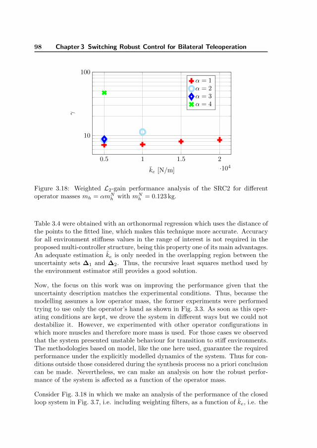
98 Chapter 3 Switching Robust Control for Bilateral Teleoperation
0.5 1 1.5 2
·104
10
100
ke [N/m]
γ
α = 1α = 2α = 3α = 4
Figure 3.18: Weighted L2-gain performance analysis of the SRC2 for differentoperator masses mh = αmN
h with mNh = 0.123 kg.
Table 3.4 were obtained with an orthonormal regression which uses the distance ofthe points to the fitted line, which makes this technique more accurate. Accuracyfor all environment stiffness values in the range of interest is not required in theproposed multi-controller structure, being this property one of its main advantages.An adequate estimation ke is only needed in the overlapping region between theuncertainty sets ∆1 and ∆2. Thus, the recursive least squares method used bythe environment estimator still provides a good solution.
Now, the focus on this work was on improving the performance given that theuncertainty description matches the experimental conditions. Thus, because themodelling assumes a low operator mass, the former experiments were performedtrying to use only the operator’s hand as shown in Fig. 3.3. As soon as this oper-ating conditions are kept, we drove the system in different ways but we could notdestabilize it. However, we experimented with other operator configurations inwhich more muscles and therefore more mass is used. For those cases we observedthat the system presented unstable behaviour for transition to stiff environments.The methodologies based on model, like the one here used, guarantee the requiredperformance under the explicitly modelled dynamics of the system. Thus for con-ditions outside those considered during the synthesis process no a priori conclusioncan be made. Nevertheless, we can make an analysis on how the robust perfor-mance of the system is affected as a function of the operator mass.
Consider Fig. 3.18 in which we make an analysis of the performance of the closedloop system in Fig. 3.7, i.e. including weighting filters, as a function of ke, i.e. the

3.4 Conclusions 99
maximal environment stiffness. The different plots correspond to different operatormasses mh = αmN
h as a function of the nominal operator mass mNh = 0.123 kg
found in Section 3.2.1, the rest of the parameters remain unchanged. For the caseα = 1, as expected the system is robustly stable for all ke <= 2.0 kN/m. For α = 2,no γ value was found for ke >= 1.5 kN/m, which means that robust performanceis not guaranteed in that region. Moreover for ke <= 1.0 kN/m a degradation inperformance is already noticeable. For α = 3 and α = 4, γ values were only foundfor ke <= 5.0 kN/m and a trend in degradation of performance can be noticed asthe operator mass increases.
Finally, we give some indications on how the uncertainty description can be im-proved to account a priori also for larger ranges of operator’s mass. It is desirableto include the operator parameters ranging from zero up to the maximum of theirvariation. This ranges from the case when the operator releases the device, up tothe case when a tight grip is performed under different arm-hand configurations.However, there are two main challenges while doing so. On one hand, when theparameters become zero, notice that the system becomes uncontrollable in termsof performance because the controller has no more effect on fh. On the otherhand, the constant multipliers utilized here for uncertainty description takes intoaccount arbitrary fast time-varying parameters, thus it introduces too much con-servatism if also the operator’s mass is made uncertain. The first issue could beaddressed by separating conditions for robust stability and for robust performance,thus having two different uncertain parameter ranges for each of them. Reductionof the conservatism in the second issue is possible via frequency-dependent, i.e.,dynamic multipliers (Megretski and Rantzer (1997)), with which is possible to im-posed bounds on the rate of variation of the operator’s parameters. These issueswill be topic of future research.
3.4 Conclusions
In this chapter we proposed a new approach towards control design for bilateralteleoperation. We used a multi-controller structure in which several robust con-trollers are scheduled according to an estimate ke of the environment stiffness. Thesynthesis results demonstrated that with the proposed Switching Robust Con-troller (SRC) we were able to improve the achieved performance in comparisonwith the case when only a single LTI robust controller is used. Simulations andexperiments validated the synthesis results, the designed SRC achieved robust per-formance for all the uncertainty region it was designed for, i.e. low mass operatorwith time-varying stiffness and time-varying environment stiffness within a widerange. Moreover, the switching among robust controllers was made in a stable andsmooth way, because they all share a common Lyapunov function.

100 Chapter 3 Switching Robust Control for Bilateral Teleoperation
In the next chapter, we propose a similar multi-controller structure, in which sta-ble switching among controllers is achieved without the requirement of a commonLyapunov function.

101
Chapter 4
Switching Robust Control viaDwell Time Conditions
IN switching robust control, stable and smooth switching among con-trollers will be guaranteed by the existence of a common Lyapunov func-
tion. In this chapter, we propose a method to further reduce conservatismin the achievable performance of switching robust control synthesis for tele-operation systems. In this approach multiple Lyapunov functions with aspecial structure are introduced, which are linked by conditions of minimumaverage dwell time switching among controllers. We show the advantageof the proposed method by means of a control design synthesis for a 1-DoFteleoperation system, and by means of simulations of the correspondingclosed loop system.
4.1 Introduction
Teleoperation systems are used to manipulate a remote environment by meansof a master and a slave device. Moreover, the use of haptic feedback can pro-vide a feeling of tele-presence to the operator. It is desirable that the systempresents high performance, e.g. the operator feels as if he/she is manipulatingthe environment directly, in a stable fashion. Nevertheless, the inherent trade-
This chapter is based on the following manuscript: Lopez Martınez, C. A., Molengraft, R.v. d., and Steinbuch, M. (2014d). Switching robust control synthesis for teleoperation via dwelltime conditions. In 9th International Conference, EuroHaptics 2014, Versailles, France. Springer.To appear online

102 Chapter 4 Switching Robust Control via Dwell Time Conditions
off between performance and (robust) stability represents a challenging problemin designing controllers that meet an appropriate balance (Hokayem and Spong(2006), Passenberg et al. (2010)). During many years the focus of the controldesign was only on stability. Therefore, passivity (Niemeyer and Slotine (1991))based methods have been widely used to design controllers that guarantee sta-bility but performance is often not taken into account. Moreover, some of thesetechniques are only applicable to Linear Time Invariant (LTI) systems, while, inpractice operator/environment dynamics are inherently time-varying and partiallybounded. Some works have explicitly addressed performance and stability whileincorporating those properties. For instance, Vander Poorten (2007) used virtualshunt dynamics to put bounds on the maximum operator impedance. In Chapter 2we have used a parametric model to include time variation and boundedness ofthe operator and the environment dynamics. This allowed us to balance trans-parency and stability during the control design process. We achieved a limitedrobustness range of environment stiffness, not fully covering realistic conditionsin applications such as minimally invasive surgery, needle insertion, etc., in whichenvironment stiffness can vary from 83N/m for fat, up to 6902N/m for the ribcagebone, see Bankman et al. (1990). Furthermore, hard contacts might be present forexample during collision between instruments. Therefore, it is desirable to furtherincrease the range of environment-related parameters for which performance andstability can be guaranteed in order to cover the requirements of real-life surgicalconditions.
To increase the region of performance, one can think about estimating the en-vironment stiffness and use such estimation to design a controller that adaptsaccordingly. Willaert et al. (2010) and Cho and Lee (2009) use environment esti-mation for bilateral teleoperation control. However they do not provide quantita-tive information on the environment stiffness range in which robust performanceis achieved, or the achieved operating range is limited to soft environment stiff-ness. Moreover, these works rely on unbiased, low noise and fast convergence ofthe estimated environment stiffness, requirements which in practice are difficult tomeet simultaneously.
In Chapter 3 we proposed the use of switching robust control. We accounted foruncertainty in the operator and environment dynamics as well as uncertainty andnoise in the estimation of the environment stiffness that is used for control schedul-ing. The controllers were designed such that they share a common quadratic Lya-punov function, which ensures stability under arbitrary fast switching betweenthem. This in fact adds conservatism since it is expected that consecutive switch-ing between controllers does not happen infinitely fast. Therefore, to decreasesuch conservatism, an average switching dwell time concept (Hespanha and Morse(1999)) can be used. Its application to control synthesis poses a challenging prob-lem due to non-linearity of the resulting conditions. Such a concept has been

4.2 Adding control design flexibility via dwell time conditions 103
already used in Kruszewski et al. (2012) for robustness against time-varying de-lays, and also in Lu et al. (2006) for LPV control of an aircraft. Based on thelatter work we propose an extension to the methods in Chapter 3, such that therequirement of a common Lyapunov function is relaxed and we find conditionsfor control synthesis that reduce the conservatism in the achievable performance.This is the first time that conditions of average dwell time are used to synthesizecontrollers in switching robust control for teleoperation systems. We validate theproposed method by means of a control design synthesis for a 1-DoF teleoperationsystem and we present simulations showing transition and contact with differentenvironments.
In Section 4.2 we briefly discuss the model of the 1-DoF teleoperation system andwe describe the framework for control synthesis of the proposed method. Sim-ulations are presented and discussed in Section 4.3. Finally, in Section 4.4 theconclusions are presented.
4.2 Adding control design flexibility via dwell timeconditions
4.2.1 Model of the teleoperation system for switching robustcontrol
Generalized plant
We use the same model as in Chapter 2 which is briefly discussed here. The modelconsists of two subsystems, an operator/master-device pair and an environment/slave-device pair. We consider master, slave devices and environments with mass-damper-spring dynamics. For the operator’s arm model, we used the same modelas the one that is identified in Chapter 2. The model is described by an impedanceZh(s), which consists of a mass-damper-spring system and a filter Qh(s) modelingthe operator’s arm-hand dynamics above 10 Hz. In such a model only the operatorstiffness kh is considered to be uncertain and time-varying. Therefore, ∆e = khrepresents the uncertainty block of the operator/master-device dynamics. Simi-larly, only the environment stiffness ke is considered uncertain. Therefore, ∆h = kerepresents the uncertainty block of the environment/slave-device pair dynamics.
Subsequently, all different components are gathered and the teleoperation is mod-eled using a so called generalized plant structure. The system model’s structureis shown in Fig. 4.1, where q and p are the signals interfacing the uncertainty

104 Chapter 4 Switching Robust Control via Dwell Time Conditions
G
∆(δ)
Kc
w z
p
u
q
y
Figure 4.1: Generalized plant.
block ∆, w the disturbances of the system, y the measured signals, u the actu-ation signals, and z the performance signals. G contains all fixed parameters ofoperator, master and slave devices. The controller Kc in this case represents thecontroller to be designed. In the model, the operator stiffness kh and the en-vironment stiffness ke are assumed to be uncertain, bounded and they are alsoconsidered time-varying to account for more realistic behavior. Thus, the numberof uncertain parameters of the system is np = 2 and the vector of uncertain pa-rameters is δ = col(δ1, δ2) with δ1 = kh, δ2 = ke. The uncertainty block is then
defined as ∆(δ(t)) =[kh(t) 0
0 ke(t)
], ∆ ∈∆, where
∆ =
{[kh 00 ke
]: kh ∈ [kh, kh], ke ∈ [ke, ke]
}.
Please see Section 2.2.1 for details.
Augmented plant model for control design
Before introducing the model used for control design, first we discuss the mainidea of switching robust control for bilateral teleoperation presented in Chapter 3.It consists of designing a specific number Nc of LTI controllers, in which thecontroller Ki, i = 1, ...Nc has an uncertainty region ∆i of robust performance,such that ∆ ⊆ ∆1 ∪ ... ∪∆Nc
. Each Ki is then activated in its corresponding
region ∆i based on an estimate ke of ke with possibly uncertainty and noise.
Thus, the uncertainty region ∆ is partitioned in Nc sub regions
∆i =
{[kh 00 kei
]: kh ∈ [kh, kh], kei ∈ [kei, kei]
}
such that ∆ ⊆∆1 ∪ ...∪∆Nc, for i = 1, ..., Nc as illustrated in Fig. 4.2. Based on
the figure, we define uncertainty vectors δ(i) = col(kh, kei), i = 1, . . . , Nc. Define

4.2 Adding control design flexibility via dwell time conditions 105
ke
... ...
kh
kei kei+1ke1 keNc = kekei+1keike1 = ke keNc
kh
kh ∆1 ∆i ∆i+1 ∆Nc
Figure 4.2: Uncertainty regions ∆i of a switching robust controller.
also the uncertainty blocks ∆i(δ(i)) =[kh 00 kei
]for i = 1, . . . , Nc such that ∆i ∈
∆i. Note that although ke is estimated, it is still considered as an uncertaintyon each sub-region ∆i. There is overlap between the regions to avoid incorrectscheduling of controllers due to uncertainty and noise in the estimation of ke, e.g.when a controller is activated in a region ∆i that does not correspond to it. Weconsider that the estimate ke of ke is given by ke = ke± ε(ke) + η(ke) where ε(ke)
represents the magnitude of the uncertainty in ke and η(ke) represents a zero-meannoise signal in the estimation whose magnitude is bounded, i.e. |η(ke)| < ηc forke ∈ [ke, ke]. The distribution of the regions is similar as in Chapter 3 and isspecified in more detail in Section 3.2.3.
Next, we need to augment the model shown in Fig. 4.1 in order to incorporate theuncertainty partitions ∆i, i = 1, . . . , Nc and a more suitable form that is usablefor control design. Consider the model diagram presented in Fig. 4.3 in which wehave augmented and partitioned the model in Fig. 4.1 in Nc augmented generalizedplants Gi. The different components of the augmented model are described in thesame way as in Section 3.2.2. We summarize the description as follows:
The blocks V and W are weighting filters described with stable LTI systems.They allow to shape in frequency domain the desired system performance. SeeSection 3.2.5 for details. w and z are weighted copies of w and z via predefinedfilters V and W respectively. That is w = V w and z = Wz. δ(i) = col(kh, kei), i =1, . . . , Nc. are the transformed version of the parameters vectors δ(i). The specific
transformation is given in Section 3.2.3. ∆i(δ(i)), i = 1, . . . , Nc is the block di-
agonal concatenation of the parameters in δ(i). The vector q and p contain the
signals interfacing the new uncertainty block ∆. Thus p(t) = ∆(δ(t))q(t). Thevariable r ∈ [0, 1] is a scaling factor that allows to scale down the uncertaintyblocks ∆i. This allows to perform an iterative process during the control designin which one starts with the nominal case r = 0, i.e. no uncertainty, and final-izes with an unscaled uncertainty set for r = 1. We will refer to a nominal plantif r = 0. If r = 1 we have that ∆i(δi) equals the dashed block in the upperpart of Fig. 4.3. T∆i
: R2np×2np , i = 1, . . . , Nc are constant matrices that allow

106 Chapter 4 Switching Robust Control via Dwell Time Conditions
G
T∆i
∆i(δ(i))
r
W
Kci
Vw zw z
u y
qp
pi qi
Gi
Figure 4.3: Set of generalized plants with weighting filters, uncertainty transfor-mation and scaling. The dashed block in the upper part equals ∆i(δ) providedr = 1.
to map one to one the uncertain parameter set ∆i to the transformed uncertainparameter set ∆i. The transformations T∆i
allows to obtain nominal values of∆i(δ
Nom(i) ) ∈∆i for r = 0. The specific transformations from matrices T∆i,i=1,...,Nc
are given in Section 3.2.3. The blocks Kci, i = 1, . . . , Nc are then the LTI con-trollers Kci(s) = Cci(Is − Aci)−1Bci + Dci, which we will identify by their statespace description by writing
Kci(s) =
[Aci BciCci Dci
], i = 1, . . . , Nc. (4.1)
One can derive a model of the generalized plant Gi for i = 1, . . . , Nc. We denoteits state space representation by the following equation:
xpqizy
=
Ai B(i)1 B(i)2 BirC(i)1 rD(i)1 rD(i)12 rE(i)1
C(i)2 D(i)21 D(i)2 E(i)2
Ci F(i)1 F(i)2 0
xppiwu
, i = 1, . . . , Nc
Uncertainty and performance description
Similarly as in Chapter 2, we will use a specific class of Integral Quadratic Con-straints (IQCs) (see Megretski and Rantzer (1997)) to model uncertainties ∆i ∈∆i. Then consider Pi as sets of symmetric matrices Pi ∈ R2np×2np that satisfy
4.2 Adding control design flexibility via dwell time conditions 107
the following IQC
∫ T0
0
(∆i(δi)qi(t)
qi(t)
)TPi
(∆i(δi)qi(t)
qi(t)
)dt ≥ 0 (4.2)
for all q ∈ L2[0, T0], T0 ∈ R+, ∆i ∈ ∆i and i = 1, . . . , Nc. The matrix Piis a so called multiplier. To describe bounded and time-varying real parametricuncertainties we used the same matrix families Pi, i = 1, . . . , Nc described inSections 1.3 and 2.2.2.
We have chosen the performance criterion based upon the L2 gain of the mappingfrom disturbance channels w to the performance channels z as is customary inmodel-based H∞ control, e.g., see Skogestad and Postlethwaite (2005). The L2
gain from w to z can be expressed in a standard form as a quadratic performancecriterion:
∫ ∞
0
(w(t)z(t)
)TPp
(w(t)z(t)
)dt < 0 for all 0 6= w ∈ L2, (4.3)
with
Pp =
(−γ2I 0
0 I
)
The standard form to describe performance in Eq. (4.3) allows the use of otherquadratic performance criteria via Pp, see, e.g., Section 1.3 and Scherer and Wei-land (2000). To keep the generality of the theory used here, we will use the symbolPp to describe our specific performance criterion.
4.2.2 Switching robust control design using multiple quadraticLyapunov functions
In Chapter 3, we designed a switching robust controller for the 1-Dof teleoperationsystem described in Appendix A. It consists of Nc = 2 controllers sharing a com-mon quadratic Lyapunov function V (x) = xTXx, with x representing the statevector of the closed loop system. This makes the overall switched system glob-ally stable in case of arbitrary fast switching between the Nc controllers (Liberzon(2003)). In this way, the design of the different Kci(s) controllers is linked to en-sure robust performance under switching of controllers and for ∆ ∈∆, given thateach controller Ki is active in its corresponding region of operation ∆i. With thismethodology, in Chapter 3 it was shown that it is possible to improve robust per-formance, as compared with the case when using a single controller. However, therequirement of a common Lyapunov function might limit the potential of the pro-posed multi-controller structure. To add additional flexibility other than havingmore than one controller, we propose the use of multiple Lyapunov functions.

108 Chapter 4 Switching Robust Control via Dwell Time Conditions
µ
τa
≤ e−λ0tVj(x(ts))
Vi(x)
Vj(x)
tts
V (x)
Figure 4.4: Interpretation of dwell time conditions
The disadvantage of the requirement of a common Lyapunov function is that itadds unnecessary conservatism. In real applications such as minimally invasivesurgery, the slave devices might encounter sudden changes in the environment,however consecutive switching of environment is not expected to take place in-finitely fast. Therefore, we might relax the requirement of a common Lyapunovfunction and allow a different one per controller, given that we guarantee specificconditions on how much they differ. In order to achieve this, we make use of theaverage dwell time concept in switching systems by Hespanha and Morse (1999).It basically states that a switched system has average dwell time τa if the averagetime between consecutive switches in the system is at least τa.
Such concept has been applied for stability analysis of switched systems, see Liber-zon (2003). Consider a switched system with Nc subsystems. Consider a switch-ing signal σ(t) ∈ {1, . . . , Nc} that determines which subsystem is active at timet. Then consider that each subsystem of the switched system has a Lyapunovfunction Vi(x) for i = 1, . . . , Nc such that
Vj(x) ≤ µVi(x), i, j = 1, . . . , Nc (4.4)
for some µ > 1. It is proven that (see Liberzon (2003), Section 3.2.2), if
∂Vi∂x
x ≤ −λ0Vi(x), i = 1, . . . , Nc (4.5)
fro some λ0 > 0, then the switched system is stable for every switching signal σwith average dwell time
τa >ln(µ)
λ0.
Eq. (4.5) guarantees a minimal exponential decay constant λ0 of the Lyapunovfunctions Vi(x), i = 1, . . . , Nc. To interpret those results, consider Fig. 4.4, inwhich there is a switching from system i to system j at the time instant ts. Thevalue of the Lyapunov function after switching has a bound given by Eq. (4.4).

4.2 Adding control design flexibility via dwell time conditions 109
Thus, because of the minimal exponential decay rate guaranteed by Eq. (4.5), afterτa seconds it is guaranteed that Vj(x) ≤ Vi(x) and it would be safe to switch toanother controller again.
Now, this same concept is applied to the robust control design for bilateral teleop-eration systems. We know that conditions on Theorem 2.1 and 3.1 come from thetheory of dissipative systems (see Section 1.3), in which basically we have that
∂V
∂xx ≤ s(w, z) (4.6)
where s(w, z) ≥ 0 is a so called supplied function which is specified by the usedperformance criterion, see also Scherer and Weiland (2000). Thus, we simply haveto extend (4.6) (applied to each closed loop i of Fig. 4.3) with the right hand sideof Eq. (4.5) to obtain
∂Vi∂x
x− s(w, z) ≤ −λ0Vi(x), λ0 > 0, i = 1, . . . , Nc, (4.7)
which implies (4.5) if the external input w = 0. Consequently, a guaranteedexponential decay rate of the function t 7→ V (x(t)) with decay rate λ0 is obtained.Then using also (4.4) and quadratic Lyapunov functions of the form Vi(x) =xTXx, i = 1, . . . , Nc we arrived to the following result:
Initially, assume we have certain Kci(s) that achieves nominal stability for each∆i for i = 1, . . . , Nc. That is for when r = 0. Moreover, let Pi, i = 1, . . . , Nc bethe sets of symmetric matrices Pi that satisfy conditions (3.3) and (3.4). Then:
Theorem 4.1. Given constants µ > 1, λ0 > 0, the closed loop systems Gi(s) ?Kci(s) with r ∈ (0, 1] shown in Fig. 4.3 are robustly stable for all ∆i ∈ r∆i withrobust quadratic performance characterized by Pp if there exist symmetric matricesXi, and symmetric matrices Pi ∈ Pi such that
Xi � 0 (4.8)
Xi � µXj (4.9)
(?)T
0 Xi 0 0 0Xi 0 0 0 00 0 λ0Xi 0 00 0 0 Pi 00 0 0 0 Pp
I 0 0Ai B(i)1 B(i)2
I 0 00 I 0C(i)1 D(i)11 D(i)12
0 0 IC(i)2 D(i)21 D(i)22
≺ 0 (4.10)

110 Chapter 4 Switching Robust Control via Dwell Time Conditions
holds for i, j = 1, . . . , Nc. Moreover, robust stability is achieved for switchingbetween the uncertain closed loop systems r∆i ? Gi(s) ?Kci(s), i = 1, . . . , Nc if theaverage dwell time
τa >ln(µ)
λ0(4.11)
The matrices Ai, B(i)m, C(i)n, D(i)mn i = 1, . . . , Nc, m, n = 1, 2 are given in (3.7)and correspond to the state space realizations of the systems obtained by closingthe loop in Fig. 4.3 with the controller Kci, such that the obtained system has asinputs the vector col(pi, w), and as outputs the vector col(qi, z). Therefore, thecontroller matrices Aci, Bci, Cci, Dci, are incorporated in the matrices in in (3.7).
Now, our goal is to find conditions that could lead us to reduce conservatism of thecontrol synthesis procedure requiring a common Lyapunov function. However anew problem arises when translating conditions in Eq. (4.9) to synthesis conditions.To illustrate this, we describe first how a standard controller synthesis procedureworks.
Similar as in Chapters 2 and 3, Eq. (4.10) is actually not a LMI when Kci, Xi andPi are unknown. It is still possible to obtain controllers via an iterative synthesisprocedure. If we iterate between a controller step to find controllers Kci and ananalysis step to find uncertainty multipliers Pi, it is possible to make Eq. (4.10) anLMI as follows. When the controllers Kci are known, Eq. (4.10) becomes already aLMI, i.e. linear in the unknown parameters Xi and Pi. However, in the case whenPi is known, two additional steps are needed to transform Eq. (4.10) into a LMI.The details of these steps are found in the work of Scherer and Weiland (2000).Here we will describe part of the first step, which is key to understand the controlsynthesis method proposed here. It consists of the congruence transformationof the Lyapunov functions Vi(x) = xTXix. Consider the next partition of thematrices Xi,
Xi =
(Xi UiUTi ∗
)and X−1
i =
(Yi ViV Ti ∗
)(4.12)
with Ui, Vi arbitrary invertible matrices that satisfy XiYi + UiVTi = I. Next, if
we apply a congruence transformation to Eq. (4.8) with matrix
YAi =
(Yi IV Ti 0
)(4.13)
it is transformed to
Xi =
(Yi II Xi
)� 0. (4.14)
4.2 Adding control design flexibility via dwell time conditions 111
In a similar way Eq. (4.10) is transformed with matrix
YBi = diag(YAi, I, I) (4.15)
to an equation that depends on the collected matrix variables vi = {Xi, Yi,Ki,Li,Mi, Ni}, where Ki, Li,Mi, Ni are transformed variables that represent the con-troller. By an additional step such equation can be made affine in its unknowns,see Section 2.2.2 for a similar procedure applied to the synthesis of a single robustcontroller. The resulting transformed equations are given here for completeness:
Define
Ai(vi) =
(AiYi +BiMi Ai +BiNiCi
Ki AiXi + LiCi
)
B(i)n(vi) =
(B(i)n +BiNiF(i)n
XiB(i)n + LiF(i)n
)
C(i)m(r, vi) =(rm(C(i)mYi + E(i)mMi) rm(C(i)m + E(i)mNiCi)
)
D(i)mn(r, vi) =(rm(D(i)mn + E(i)mNiF(i)n)
)
for m,n = 1, 2. i = 1, . . . , Nc. r1 = r and r2 = 1. Define also
B(i)l(v) =
Ai(v) B(i)1(v) B(i)2(v)C(i)1(v) D(i)11(v) D(i)12(v)C(i)2(v) D(i)21(v) D(i)22(v)
Al = col(I, (I 0 0));
Q(i)l = diag(0, Qi, Qp, λ0Xi)
S(i)l = col(diag(I, Si, Sp), 0)
U(i)l = diag(I,R−1i , R−1
p )
Tl = diag(0, I, I)
for i = 1, . . . , Nc. Then Eq. (4.10) is equivalent to(ATl Q(i)lAl +ATl S(i)lB(i)l(v) +B(i)l(v)TST(i)lAl B(i)l(v)TTl
TTl B(i)l(v) −U(i)l
)≺ 0,
i = 1, . . . , Nc (4.16)
Now, the main inconvenience with Theorem 4.1 to arrive at synthesis conditionscomes from the fact that we can not apply a congruence transformation with YAito Eq. (4.9) because it involves different indexes i, j. One can think of treatingonly equation (4.9) without transformation. Thus, from (4.12) we get the followingequation for Xi:
Xi =
(Xi UiUTi −UTi YiV −Ti
)(4.17)
112 Chapter 4 Switching Robust Control via Dwell Time Conditions
The non-linear lower-right term in Eq. (4.17) poses an issue to make the synthesisprocess solvable with LMIs. To solve this issue, we use the same trick applied byLu et al. (2006), which is described in the following paragraphs.
First, one can select Vi = Yi and therefore Ui = Y −1i −Xi, thus Xi in Eq. (4.17)
becomes
Xi =
(Xi Y −1
i −Xi
Y −1i −Xi Xi − Y −1
i
)(4.18)
which can be written as
Xi =
(I −I0 I
)(Y −1i 00 Xi − Y −1
i
)(I −I0 I
)T.
Therefore, partitioning the closed loop state vector as x = col(xp, xc), where xpand xc are the state vectors of the plant and controller respectively, the quadraticLyapunov functions Vi(x) becomes:
Vi(x) = xTp Y−1i xp + (xc − xp)T (Xi − Y −1
i )(xc − xp) (4.19)
In this partition xp and xc have the same dimension. This is indeed the case whenthe nominal controller is designed with the same methods proposed here.
Now, note that conditions in Eq. (4.4) are only necessary at the moment of switch-ing. Therefore, if at the switching moments the controller state vector is reset toxc = xp, the Lyapunov function at the switching instant becomes
Vi([xp, xp]T ) = xTp Y
−1i xp (4.20)
Next, if (4.14) holds, from partition in (4.12) we can conclude that Yi � 0 andtherefore Y −1
i � 0, which can be substituted in condition (4.9) to obtain
Y −1i � µY −1
j , i, j = 1, . . . , Nc.
Finally, we can also conclude that
Yi � µYj , i, j = 1, . . . , Nc, (4.21)
which are conditions affine in (Yi, Yj) that can be used together with conditionsin (4.14) and (4.16) to synthesize controllers Kci, given that Pi is known and thatthe controller state is reset to xc = xp at the switching instants.
We formalize the result by the following synthesis theorem.

4.2 Adding control design flexibility via dwell time conditions 113
Theorem 4.2. For given Pi ∈ Pi and given constants µ > 1, λ0 > 0. There existcontrollers Kci(s) and Lyapunov certificates Xi as in (4.18) such that the closedloop systems Gi(s) ?Kci(s) are robustly stable for all ∆i ∈ r∆i with r ∈ (0, 1] andwith robust quadratic performance characterized by Pp if there exist variables vi =(Xi, Yi,Ki, Li,Mi, Ni) such that (4.14), (4.21) and (4.16) hold for i, j = 1, . . . , Nc.Moreover, robust stability is achieved for switching between the uncertain closedloop systems r∆i ? Gi(s) ? Kci(s), i = 1, . . . , Nc if the average dwell time
τa >ln(µ)
λ0
provided that the controller is reset to xc = xp when a switching occurs.
The matrices of the state space representation of each Kci(s) are then computedusing the following equation
(Aci BciCci Dci
)
=
(Ui XiBi0 I
)−1(Ki −XiAiYi Li
Mi Ni
)(V Ti 0CiYi I
)−1
(4.22)
with Vi = Yi and Ui = Y −1i −Xi.
Before summarizing the iterative synthesis procedure, for the robust analysis stepswe need Lyapunov certificates Xi compatible with those obtained with Theo-rem 4.2, i.e. Xi with structure as in (4.18). Therefore, to obtain Pi when Ki
is known, we use the following theorem.
Theorem 4.3. Given given constants µ > 1, λ0 > 0 and controllers Kci(s), theclosed loop systems Gi(s) ? Kci(s) with r ∈ (0, 1] shown in Fig. 4.3 are robustlystable for all ∆i ∈ r∆i with robust quadratic performance characterized by Pp ifthere exist symmetric matrices Xi � 0, YIi = Y −1
i � 0 ,and symmetric matricesPi ∈ Pi such that
Xi =
(Xi YIi −Xi
YIi −Xi Xi − YIi
)� 0 (4.23)
YIi � µYIj (4.24)
and (4.10) hold for i, j = 1, . . . , Nc. Moreover, robust stability is achieved forswitching between the uncertain closed loop systems r∆i ? Gi(s) ? Kci(s), i =1, . . . , Nc if the average dwell time
τa >ln(µ)
λ0
114 Chapter 4 Switching Robust Control via Dwell Time Conditions
provided that the state of the controller is reset to xc = xp when a switching occurs.
We finally summarize the synthesis procedure as follows. We define each region∆i, transform it and scale in the same way as in the methods in Chapter 3.Then, without loss of generality, the uncertainty parameters can be transformedinto new parameters kh ∈ [0, 1], kei ∈ [0, 1] such that transformed uncertainty
becomes ∆i =
[kh 0
0 kei
]. Then, we design first a nominal controller for r = 0,
by using Theorem 4.2 after removing the uncertainty channels. Then, we iteratethe following steps:
� for fixed Ki, maximize r using the bisection algorithm and get the corre-sponding matrices Pi by using Theorem 4.3 while minimizing γ, keepingγ < γ, for a certain γ.
� for fixed Pi, maximize r using the bisection algorithm and get the corre-sponding controllers Kci by using Theorem 4.2 while minimizing γ, keepingγ < γ, for a certain γ.
� Once r = 1 is achieved, we iterate the two previous steps and on each theperformance level γ is minimized until no further progress can be made.
The value γ is introduced such that at the initial steps of the iterative synthesisprocedure we allow γ to be large. This allows to avoid local minima around smallvalues of the uncertainty scaling r. Then, after reaching r = 1 we minimize γ.Details on the iterative procedure are given in Appendix B, from which we haveused the version II of the iterative procedure.
Now, the reset conditions introduced here helped to relax the requirement of acommon Lyapunov function. However, the actual implementation of such resetposes two issues. Firstly, it requires the implementation of an observer that couldfollow abrupt changes accurately and in a robustly stable fashion. Secondly, evenif we implement such observer, sudden high frequency peaks might be introducedwhen resetting the controller state, which in theory does not represent an issuefor stability since the total Lyapunov function remains decreasing, however un-modeled dynamics can be excited in practice leading to instability. In fact suchpeaks were observed in simulation. A solution to avoid those issues is not toperform the controller state reset at the moment of switching. All we have to do isto perform a final analysis using Theorem 4.1, take r = 1 and minimize γ. In facteven less conservative results are obtained in the analysis since we do not have toenforce a particularly structure in Xi. Thus, the reset conditions are only used tobe able to have a synthesis procedure based on LMI’s that relax the requirementof a common Lyapunov function.
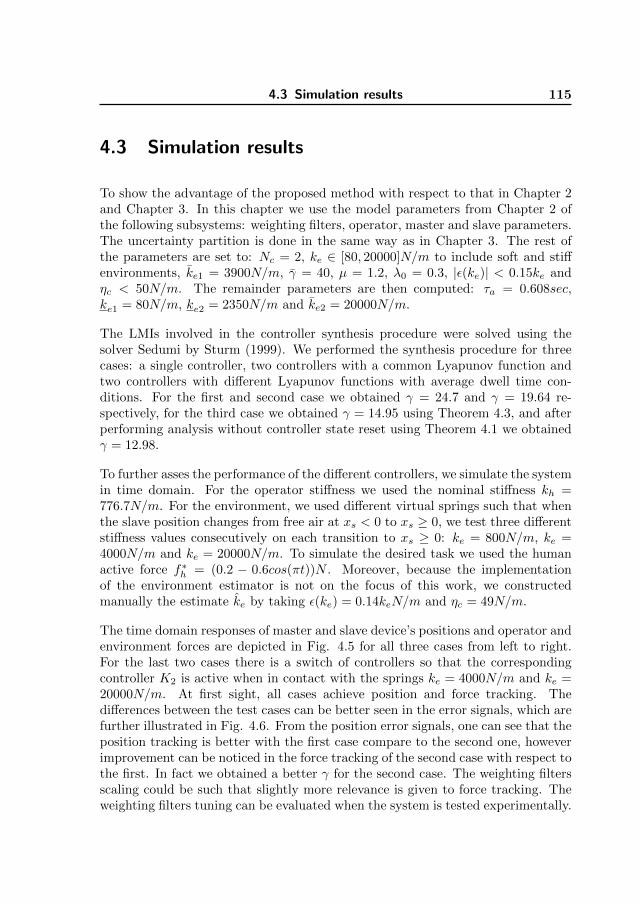
4.3 Simulation results 115
4.3 Simulation results
To show the advantage of the proposed method with respect to that in Chapter 2and Chapter 3. In this chapter we use the model parameters from Chapter 2 ofthe following subsystems: weighting filters, operator, master and slave parameters.The uncertainty partition is done in the same way as in Chapter 3. The rest ofthe parameters are set to: Nc = 2, ke ∈ [80, 20000]N/m to include soft and stiffenvironments, ke1 = 3900N/m, γ = 40, µ = 1.2, λ0 = 0.3, |ε(ke)| < 0.15ke andηc < 50N/m. The remainder parameters are then computed: τa = 0.608sec,ke1 = 80N/m, ke2 = 2350N/m and ke2 = 20000N/m.
The LMIs involved in the controller synthesis procedure were solved using thesolver Sedumi by Sturm (1999). We performed the synthesis procedure for threecases: a single controller, two controllers with a common Lyapunov function andtwo controllers with different Lyapunov functions with average dwell time con-ditions. For the first and second case we obtained γ = 24.7 and γ = 19.64 re-spectively, for the third case we obtained γ = 14.95 using Theorem 4.3, and afterperforming analysis without controller state reset using Theorem 4.1 we obtainedγ = 12.98.
To further asses the performance of the different controllers, we simulate the systemin time domain. For the operator stiffness we used the nominal stiffness kh =776.7N/m. For the environment, we used different virtual springs such that whenthe slave position changes from free air at xs < 0 to xs ≥ 0, we test three differentstiffness values consecutively on each transition to xs ≥ 0: ke = 800N/m, ke =4000N/m and ke = 20000N/m. To simulate the desired task we used the humanactive force f∗h = (0.2 − 0.6cos(πt))N . Moreover, because the implementationof the environment estimator is not on the focus of this work, we constructedmanually the estimate ke by taking ε(ke) = 0.14keN/m and ηc = 49N/m.
The time domain responses of master and slave device’s positions and operator andenvironment forces are depicted in Fig. 4.5 for all three cases from left to right.For the last two cases there is a switch of controllers so that the correspondingcontroller K2 is active when in contact with the springs ke = 4000N/m and ke =20000N/m. At first sight, all cases achieve position and force tracking. Thedifferences between the test cases can be better seen in the error signals, which arefurther illustrated in Fig. 4.6. From the position error signals, one can see that theposition tracking is better with the first case compare to the second one, howeverimprovement can be noticed in the force tracking of the second case with respect tothe first. In fact we obtained a better γ for the second case. The weighting filtersscaling could be such that slightly more relevance is given to force tracking. Theweighting filters tuning can be evaluated when the system is tested experimentally.

116 Chapter 4 Switching Robust Control via Dwell Time Conditions
Nc=
1
position (mm)
−5 0 5
force (N)
time (sec)
23
45
67
0 5 10
Nc=
2,CommonLyap.
time (sec)
23
45
67
Nc=
2,Dwell
T.Lyap.
xs
xm
time (sec)
23
45
67
fe
fh
Fig
ure
4.5
:T
ime
dom
ainresp
onses
ofp
ositions
and
operator
forcesw
hen
usin
gd
ifferen
tco
ntrol
synth
esism
ethod
s.T
hree
enviro
nm
ent
stiffn
essare
tested,
the
grayareas
show
wh
enth
eslave
isin
conta
ctw
ithth
een
viron
men
t.

4.3 Simulation results 117
xm−xe(m
m)
−0.5
0
0.5
f h−f e(N
)
time (sec)
2 3 4 5 6 7
−0.5
0
0.5
1
Nc = 1Nc = 2, Comm. Lyap.Nc = 2, Dwell T. Lyap.
Figure 4.6: Force and position error responses. Gray areas indicate contact withenvironment.
Now, using the controller synthesized with the method proposed here, one can seethat in general both position and force tracking are improved with respect to theother two cases. The improvement is especially noticeable in the force trackingsignals after the peak response following the controller switching. However, anincrease in the peak force right after contact with the different environments isobserved for the controller proposed here.
When the slave device is in free air, the smaller the magnitude of the force feltby the operator, the better is the haptic feeling of free air, and it is improved bythe last two controllers in comparison with the case where a single controller isused. Moreover, one can see that all the controllers can handle the transition fromke = 0N/m to ke = 20000N/m, representing a hard contact.
As a last remark, the controller here designed guarantees robust stability giventhat the switching sequence satisfies the minimum average dwell time. Under thespecific testing scenarios presented here, simulations showed that the transitionsare stable. However, one can wonder whether there is any guarantee that thesystem will always present stable transitions and satisfy the average dwell time.In theory, the theorems presented here do not guarantee that explicitly becausesmoothness during the switching is not guaranteed. For instance, large value ofµ gives more freedom during the control design which can improve the perfor-mance level γ. However, for large values of µ, the procedure would get closeto the case of having independent Lyapunov functions, for which a direct switchamong controllers would cause oscillatory behavior that may compromised the

118 Chapter 4 Switching Robust Control via Dwell Time Conditions
stability. Therefore, there is a trade-off between a smooth transition guaranteedby a common Lyapunov function and an improved performance level γ obtainedvia multiple and independent Lyapunov functions. Moreover, a large value of λ0
results in an increased rate of decay of the Lyapunov functions Vi, which can bebeneficial to rapidly reject transient responses after controller switching. However,there might not exist a controller that results in a large value of λ0 and also meetsthe requirements imposed on the actuation signals via the weighting filters.
In fact, initial exploratory experiments were performed with the controller pro-posed here. For some tests, the increased peak forces in the system’s response,after contact with the environment, made the operator to react in such a way thatthe average dwell time was not satisfied. Hence, it would be interesting to studyin depth the effect of the design variables µ and λ0 not only on γ, but also on thetime-domain response (in simulations and experiments) during the transition aftercontroller switching.
4.4 Conclusions
In this chapter, we have proposed a new methodology for control synthesis of aswitching robust controller for bilateral teleoperation. It is not required to havea common Lyapunov function among its controllers but instead the controllersare linked with a condition based on average dwell time switching. The synthe-sis results showed already that we can achieve a lower L2 gain γ using the newrelaxed conditions. Moreover, simulations confirmed the expected improvementin position and force tracking with respect to the case where a single controllerand two controllers with a shared Lyapunov function are used. Thus the resultsdemonstrated the potential of the approach towards increasing performance of thesystem.
In the next chapter, we will introduce a multi-controller structure that allows forindependent performance optimization of its different robust controllers.

119
Chapter 5
Bumpless Transfer of RobustControllers for Teleoperation
IN THIS CHAPTER we propose a controller scheme with multiple ro-bust controllers in which every controller is performance-optimized sep-
arately. The switching among them is based on bumpless transfer and theyare scheduled using an environment stiffness estimator. Limited accuracyand noise of such estimator is also taken into account during control de-sign. We show the applicability of the approach by experiments on a 1-DOFteleoperated system.
5.1 Introduction
Bilateral teleoperation systems are intended to provide a feeling of tele-presenceusing force feedback while an operator manipulates a remote environment by meansof a master and a slave device. It is desirable that the system presents high per-formance, e.g. the operator feels as if he/she is manipulating the environmentdirectly, in a stable fashion. However, the inherent trade-off between performanceand (robust) stability represents a challenging problem in designing controllersthat meet an appropriate balance, see, e.g., Hokayem and Spong (2006), Passen-berg et al. (2010). Passivity (Niemeyer and Slotine (1991)) based methods havebeen widely used to design controllers that guarantee stability but performance
This chapter is based on the following manuscript: Lopez Martınez, C. A., Molengraft, R.v. d., and Steinbuch, M. (2014a). High performance teleoperation by bumpless transfer of robustcontrollers. In IEEE Haptics Symposium 2014, pages 209–214, Houston, TX, U.S.A

120 Chapter 5 Bumpless Transfer of Robust Controllers for Teleoperation
is not taken into account. On the other hand, operator/environment dynamicsare inherently time-varying, operator dynamics are bounded and in many appli-cations environment parameters such as mass, damping and stiffness are boundedas well. Such properties are often not taken into account explicitly. Some workshave addressed performance and stability while incorporating knowledge on op-erator/enviroment bounded dynamics. For instance, in Vander Poorten (2007)the author used virtual shunt dynamics to put bounds on the maximum operatorimpedance. In the methods presented in Chapter 2, we included such proper-ties during the control design process to balance transparency and stability. Wealso experimentally validated the design of a robust Linear Time Invariant (LTI)controller, which yields a high performance for time-varying environment stiffnessin a limited range. However, for applications such as minimally invasive surgery,needle insertion, etc., environment stiffness can vary from 83N/m for fat, up to2483N/m for bone (see Gerovich et al. (2004)) and even up to 6902N/m for theribcage (see Bankman et al. (1990)). Furthermore hard contacts might be presentfor example by collision between instruments. Therefore, it is desirable to furtherincrease the range in which performance and stability is achieved in order to coverthe requirements of real-life surgical conditions.
In many cases there is no guarantee that a single LTI controller exists that ensuresboth high performance and stability for a wide range of environment stiffnessvalues. In case such controller exists, finding it involves a non-convex optimizationprocess, see, e.g., Vander Poorten (2007) and Chapter 2, which might lead toa local optimum. To increase the region of performance, one can think aboutestimating the environment stiffness and use such estimation to design a controllerthat adapts accordingly. Some works, e.g. Willaert et al. (2010), Cho and Lee(2009), use environment estimation for bilateral teleoperation control. Howeverthey do not provide quantitative information on the environment stiffness range inwhich robust performance is achieved, or the achieved operating range is limited tosoft environment stiffness bellow 500N/m. Moreover, these works rely on unbiased,low noise and fast convergence of the estimated environment stiffness, requirementswhich in practice are difficult to meet simultaneously.
Switching control could provide a solution to the problem into consideration. Someexisting switching control methods suggest to switch between different operatingpoints of the overall system, see, e.g., Leith and Leithead (2000), Liberzon (2003),but uncertainty in the parameters is not taken into account or stable switchingis not guaranteed. Multiple model adaptive control, which is also a switchingbased method, has been used in teleoperation in Shahdi and Sirouspour (2005).However performance is not guaranteed and the results exhibit undesired highfrequency responses. We have already explored switching robust control techniquesin Chapters 3 and 4. We designed switching robust controllers that account foruncertainty in the operator and environment dynamics, as well as uncertainty

5.2 Bumpless transfer in bilateral teleoperation 121
and noise in the estimation of the environment stiffness that is used for controlscheduling. In Chapter 3, the controllers were designed such that they share acommon quadratic Lyapunov function, which ensures stable and smooth switchingamong them. In Chapter 4, the requirement of a common quadratic Lyapunovfunction was relaxed. Instead, different Lyapunov functions are used that arelinked using conditions from a minimum average dwell time requirement.
Therefore in this chapter we propose a controller scheme similar as in Chapters 3and 4, with the main difference that every controller is designed separately andthe switching among them is based on bumpless transfer (see Zaccarian and Teel(2005)). In this way we avoid the conservatism added by requiring conditions link-ing the different Lyapunov functions, yet achieving stable switching. This allowsto optimize the performance of each controller in its respective range of operation.Moreover, we implemented the whole scheme experimentally, including the bump-less compensator and an environment estimator capable of following rapid changesin the environment stiffness. This is the first time that experiments are presentedin teleoperation using switching of robust controllers by bumpless transfer. In sucha way, robust performance is guaranteed while interacting with different types ofenvironments, either with soft or with stiff environments. Furthermore, when theenvironment changes from one type to the other, the switch between the under-lying controllers is done such that high frequency peaks in the system’s responseare avoided.
In Section 5.2 we describe the framework for control design and implementationof the proposed controller scheme. Experiments are presented and discussed inSection 5.3. Finally, in Section 5.4 the conclusions are presented.
5.2 Bumpless transfer in bilateral teleoperation
5.2.1 Linear fractional representation of a teleoperation system
To formulate the synthesis problem of our switching controller, we first describethe teleoperation system model. It was already presented in Chapter 2 and it isbriefly discussed here. The model consists of two subsystems, operator/master-device pair and environment/slave-device pair. We consider master, slave devicesand environments with mass-damper-spring dynamics. For the operator’s armmodel, we used the same model identified in Chapter 2. The model is describedby an impedance Zh(s), which consists of a mass-damper-spring system and afilter Qh(s) modeling the operator’s arm-hand dynamics above 10 Hz. In such amodel only the operator stiffness kh is considered to be uncertain and time-varying.

122 Chapter 5 Bumpless Transfer of Robust Controllers for Teleoperation
G W
∆(δ)
V
Kc
w zw z
p
u
q
yGw
Figure 5.1: Generalized plant with weighting filters.
Therefore, ∆h = kh represents the uncertainty block of the operator/master-devicedynamics. Similarly, only the environment stiffness ke is considered uncertain.Therefore, ∆h = ke represents the uncertainty block of the environment/slave-device pair dynamics.
Subsequently, all different components are gathered and the teleoperation is mod-eled using a so called generalized plant structure. The system model’s structureis shown in Fig. 5.1, where q and p are the signals interfacing the uncertaintyblock ∆, w the disturbances of the system, y the measured signals, u the actu-ation signals, and z the performance signals. G contains all fixed parameters ofoperator, master and slave devices. The controller Kc in this case represents thecontroller to be designed. In the model, the operator stiffness kh and the en-vironment stiffness ke are assumed to be uncertain, bounded and they are alsoconsidered time-varying to account for more realistic behavior. Thus, the numberof uncertain parameters of the system is np = 2 and the vector of uncertain pa-rameters is δ = col(δ1, δ2) with δ1 = kh, δ2 = ke. The uncertainty block is then
defined as ∆(δ(t)) =[kh(t) 0
0 ke(t)
], ∆ ∈∆, where
∆ =
{[kh 00 ke
]: kh ∈ [kh, kh], ke ∈ [ke, ke]
}.
V and W are weighting filters described with stable LTI systems. They allow toshape in frequency domain the desired system performance. See Section 3.2.5 fordetails. w and z are weighted copies of w and z via predefined filters V and Wrespectively. That is w = V w and z = Wz.
Finally, for the actual implementation of the synthesis procedure, a transformationof the parameters and a scaling are used. Please see Section 2.2.1 for details.

5.2 Bumpless transfer in bilateral teleoperation 123
5.2.2 Uncertainty region distribution and robust control design
In Chapter 2, using Linear Matrix Inequalities (LMI’s) (Scherer and Weiland(2010)), we synthesized a single LTI robust controller with robust performanceoperation for environment stiffness ke up to ≈ 3000N/m. In order to increase theoperational range of environment stiffness and being able to deal with stiff envi-ronments, we propose the use of a multi robust-controller structure that schedulesdifferent robust controllers according to the estimate ke of ke. The idea is to de-sign certain number Nc of LTI robust controllers, in which the ith controller hasan uncertainty region ∆i of robust performance, such that all regions combinedcovers the desired region ∆.
A similar framework has been presented in Chapters 3 and 4. The method pre-sented here differs in two main points. Firstly, the switching strategy in Chapter 3is based on the existence of a common Lyapunov function, which might not existor in order to find it we might have to sacrifice performance. In Chapter 4 theLyapunov functions involved in the control synthesis are linked using dwell timeconditions, which could still introduce conservatism in the achievable performance.The switching here is based on bumpless transfer (see Zaccarian and Teel (2005)and references therein) and does not require conditions linking the involved Lya-punov functions. This allows for independent performance optimization of eachcontroller. Secondly, in the methods in Chapters 3 and 4 the partition of the wholeuncertainty has to be made prior to the controller synthesis, increasing the num-ber of variables to be defined beforehand. Here instead, only the whole desireduncertainty region and a desired level of performance need to be defined, becausethe synthesis algorithm proposed here finds automatically a distribution of theregions.
The methodology consists on designing a certain number Nc of robust controllers,which will be determined by the synthesis algorithm itself. In order to divide theuncertainty region ∆ into sub-regions ∆i, i = 1, ..., Nc, we define Nc uncertainty
blocks ∆i such that ∆i =
[kh 00 kei
]for i = 1, ..., Nc and ∆i ∈ ∆i, where the
class ∆i =
{[kh 00 kei
]: kh ∈ [kh, kh] ∧ kei ∈ [kei, kei]
}and ∆ ⊆∆1∪...∪∆Nc .
Such partition is depicted in Fig. 5.2. There is overlap between the regions toavoid chattering behavior due to noise and to avoid wrong scheduling of controllersdue to uncertainty and noise in the estimation of ke. To illustrate this, considerthat the estimate ke of ke is given by:
ke = ke ± ε(ke) + η(ke) (5.1)
where ε(ke) represents the magnitude of the uncertainty in ke and η(ke) representsthe zero-mean noise signal in the estimation such that |η(ke)| < ηc for ke ∈ [ke, ke].
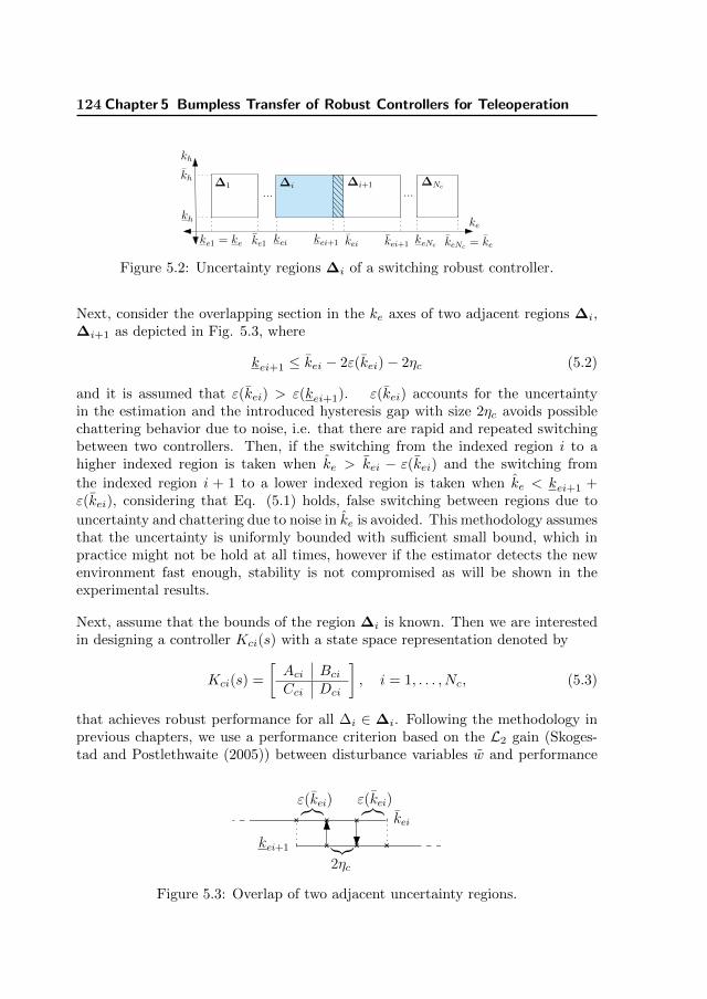
124 Chapter 5 Bumpless Transfer of Robust Controllers for Teleoperation
ke
... ...
kh
kei kei+1ke1 keNc = kekei+1keike1 = ke keNc
kh
kh ∆1 ∆i ∆i+1 ∆Nc
Figure 5.2: Uncertainty regions ∆i of a switching robust controller.
Next, consider the overlapping section in the ke axes of two adjacent regions ∆i,∆i+1 as depicted in Fig. 5.3, where
kei+1 ≤ kei − 2ε(kei)− 2ηc (5.2)
and it is assumed that ε(kei) > ε(kei+1). ε(kei) accounts for the uncertaintyin the estimation and the introduced hysteresis gap with size 2ηc avoids possiblechattering behavior due to noise, i.e. that there are rapid and repeated switchingbetween two controllers. Then, if the switching from the indexed region i to ahigher indexed region is taken when ke > kei − ε(kei) and the switching from
the indexed region i + 1 to a lower indexed region is taken when ke < kei+1 +ε(kei), considering that Eq. (5.1) holds, false switching between regions due to
uncertainty and chattering due to noise in ke is avoided. This methodology assumesthat the uncertainty is uniformly bounded with sufficient small bound, which inpractice might not be hold at all times, however if the estimator detects the newenvironment fast enough, stability is not compromised as will be shown in theexperimental results.
Next, assume that the bounds of the region ∆i is known. Then we are interestedin designing a controller Kci(s) with a state space representation denoted by
Kci(s) =
[Aci BciCci Dci
], i = 1, . . . , Nc, (5.3)
that achieves robust performance for all ∆i ∈ ∆i. Following the methodology inprevious chapters, we use a performance criterion based on the L2 gain (Skoges-tad and Postlethwaite (2005)) between disturbance variables w and performance
kei
kei+1
ε(kei)
︸︷︷︸
︷︸︸︷ ︷︸︸︷ε(kei)
2ηc
Figure 5.3: Overlap of two adjacent uncertainty regions.

5.2 Bumpless transfer in bilateral teleoperation 125
variables z. This gain is denoted by γ. Furthermore, it is desirable to obtain amaximum gain γ that defines the minimum performance level that we want toachieve for each closed loop of the multi robust-controller structure. To this end,we can apply the synthesis process described in Chapter 2 and further detailed inAppendix B (see version I of the procedure).
Finally, in order to fully determine the regions ∆i, we propose a sequential proce-dure. We start by the synthesis of the first controller Kc1(s). We define ke1 = keand we maximize ke1 using a bisection algorithm while keeping the performancegain of the first controller γ1 ≤ γ. Once that is done, we continue with the con-troller design of Kc2(s). By using the minimum amount of overlap as in Eq. (5.2),we define ke2 = ke1−2ε(ke1)−2ηc and maximize ke2 using bisection again keepingthe performance gain of the second controller γ2 ≤ γ. The procedure is repeateduntil we achieve kei = ke, thus we have covered the whole uncertainty region ∆.
Now, the controllers Kci(s) guarantee robust performance for each region ∆i sepa-rately. In order to couple the regions, we switch between the controllers as neededby using bumpless transfer.
5.2.3 Bumpless transfer between robust controllers
There are no a priori conditions that guarantee a stable switching between thecontrollers Kci(s). Therefore a suitable strategy must be used. If a direct switchof controllers is done, the initial condition of the state of the new controller mightcause discontinuities and large peaks in the control signal. This can generate highfrequency peaks in the system’s response at the moment of switching. To decreasesuch behavior, we use the same idea as in bumpless transfer in Zaccarian and Teel(2005). Basically, the idea is to keep the off-line controllers virtually in the loop bymeans of simulation. Each off-line controller put in a virtual loop with an internalmodel, and such loop is perturbed using signals of the real system. The result isthat at the moment the switching occurs, the state of the new on-line controlleris compatible with the new environment, allowing that undesirable high frequencypeaks in the system’s response are decreased. In Zaccarian and Teel (2005) theyused the concept for non uncertain plants. In our case, the plant presents largeuncertainty, however the controllers designed here can deal with rapid changes inthe plant within certain region. This motivated us to implement the bumplesstransfer as depicted in Fig. 5.4, in which Kci represents the controller currentlyon-line and Kcj any of all the other controllers that remain off-line. The bumplesscompensator for Kcj consists then by a plant out of the corresponding group ofplants for which the controller is robust to. Therefore, we use the same model G
as in Fig. 5.1 and we select a single element ∆ = ∆Bj =
[kBh 00 kBej
]from the
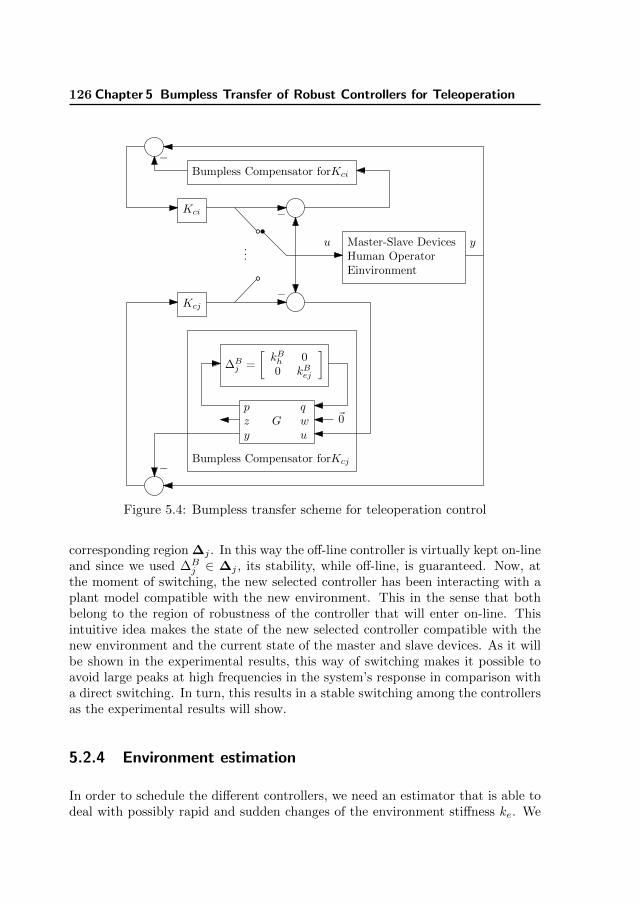
126 Chapter 5 Bumpless Transfer of Robust Controllers for Teleoperation
Master-Slave DevicesHuman OperatorEinvironment
Bumpless Compensator forKci
−
Kci −
−Kcj
...
Bumpless Compensator forKcj
∆Bj =
[kBh 00 kBej
]
Gpzy
qwu
~0
−
u y
Figure 5.4: Bumpless transfer scheme for teleoperation control
corresponding region ∆j . In this way the off-line controller is virtually kept on-lineand since we used ∆B
j ∈ ∆j , its stability, while off-line, is guaranteed. Now, atthe moment of switching, the new selected controller has been interacting with aplant model compatible with the new environment. This in the sense that bothbelong to the region of robustness of the controller that will enter on-line. Thisintuitive idea makes the state of the new selected controller compatible with thenew environment and the current state of the master and slave devices. As it willbe shown in the experimental results, this way of switching makes it possible toavoid large peaks at high frequencies in the system’s response in comparison witha direct switching. In turn, this results in a stable switching among the controllersas the experimental results will show.
5.2.4 Environment estimation
In order to schedule the different controllers, we need an estimator that is able todeal with possibly rapid and sudden changes of the environment stiffness ke. We

5.2 Bumpless transfer in bilateral teleoperation 127
Figure 5.5: Estimator with Change Detection
make use of the same estimator as in Chapter 3, which is an estimator proposedin Gustafsson (2000). The structure of the estimator is shown in Fig. 5.5. Theworking principle of this estimator is as follows: the filter block processes thediscrete inputs uk and outputs yk of a system described by a model (in our case an
environment model) to get an estimate θk of certain parameters θk (the parametersof our environment model). Then, the signal εk is used to detect abrupt changesin the parameters and under certain criteria, the detector block sends an alarm tothe filter to adapt quickly to the changes. Following the guidelines in Gustafsson(2000), the different blocks are described below.
Environment model as a linear regression model
We write our environment model in the following form
yk = ϕTk θk + ek
where k denotes sampled time instants, yk is the measured environment force, ek isthe corresponding noise, the environment parameters vector is θk = col(ke(k), f∗e (k))with f∗e (k) being the active component of the environment force, and the so calledregression vector ϕk is given by ϕk = col(uk, 1) with uk = xs(k) being the positionof the slave device.
Filter
For the filter block we utilize a Kalman filter for linear regressions, which is im-plemented in its recursive form as follows:
ϕk = col(uk, 1)
Kk =Pk−1ϕk
Rk + ϕTk Pk−1ϕk
Pk = Pk−1 −Pk−1ϕkϕ
Tk Pk−1
Rk + ϕTk Pk−1ϕk+Qk
θk = θk−1 +Kk(yk − ϕTk θk−1)
εk = yk − ϕTk θk

128 Chapter 5 Bumpless Transfer of Robust Controllers for Teleoperation
where θk is the estimated vector of the environment model parameters, Rk is takenas 1 without loss of generality and Qk is a design parameter that determines thespeed of converge of the filter. Large values of Qk make the filter to react fasterbut also the estimate will have more noise. The variable εk is the error betweenthe actual measurement and the reconstructed measurement obtained with θk.
Detector
The detector block is defined as a threshold function in order to decide when tomake the filter to react fast. Thus, when |εk| < L|εk|, no alarm is generated and weuse Qk = Qnom. When |εk| ≥ L|εk|, it means that yk has deviated too much fromthe true measurement and the filter must adapt rapidly to the new environmentby setting Qk = Qfast.
Therefore, the estimator is tuned via L|εk|, Qnom and Qfast. This tuning is es-sential to be able to detect abrupt changes fast enough to schedule on time thecontrollers of the multi-controller structure.
5.3 Experimental results on a 1-DoF academic setup
Experiments were carried out on the setup described in Appendix A. For themaster-slave devices, the operator and the weighting filters we have used the sameparameters as in Chapter 2. The environment estimator parameters were ex-perimentally determined, we used Qnom = diag(1, 0.01), Qfast = diag(107, 1),L|εk| = 1.0 N, |ε(ke)| ≤ 0.15ke and ηc = 50N/m which gave us good results inpractice. We used a desired range for ke ∈ [80, 40000]N/m to include both softand stiff environments as in hard contacts. Finally, we selected γ = 5.
The LMIs involved in the controller synthesis procedure were solved using thesolver Sedumi (see Sturm (1999)). Because variation in mh is not considered,making the design for its nominal value mN
h = 0.53kg can cause instability whenthe master device is in free air (see Chapter 2). One possible solution to thatproblem is to make the design for a reduced mass mh = rmm
Nh , rm ∈ [0, 1]. The
side effect is that there will be a decrease in performance due to the bandwidthreduction. We proceed the design with mh = 0.3mN
h which gave us stability infree air. Then, after applying the complete synthesis procedure we obtained intotal two controllers with γ1 = 4.45, ke1 = 80N/m, ke1 = 3897N/m, γ2 = 4.46,ke2 = 2630N/m and ke2 = 40000N/m.
For implementation, all controllers were discretized using the tustin method with

5.3 Experimental results on a 1-DoF academic setup 129
0
2000
4000
6000Stiffness(N
/m)
ke
48 49 50 51
−1
−0.5
0
0.5
1
Force(N
)
time [sec]
ε
Figure 5.6: Environment estimator responses to different materials
a sample period Ts = 5 × 10⁻⁴sec.. For the bumpless compensators we selectedkBh = 776.7N/m, kBe1 = 80N/m and kBe2 = 4000N/m, which are arbitrary choices.To perform the experiments, different materials are located such that the slavedevice enters in contact with them as shown in Fig. A.1. Initially the operatormoves the master such that the slave device is in free air, then it comes initiallyin contact with a soft spring. The procedure is consecutively repeated for a stifffoam and for a piece of metal.
First, we analyze the response of the environment estimator shown in Fig. 5.6.One can see that indeed the environment estimator adapts rapidly to the newenvironment, confirming the suitability of the selected estimator structure. At themoments in which the environment changes, one can also notice that |ε| ≥ 1.0and immediately after the filter is reset, it follows a fast convergence transient andtherefore a decrease in ε. However, some peaks in ke are seen before convergencewhich are not present if the system is simulated. More insight is required tounderstand that phenomenon and will be study in the future.
Next, the time domain results of positions and forces of the system are illustratedin Fig. 5.7. The bottom plot shows the index of the current on-line controller.Regarding the performance after transitions and while in contact with the differentenvironments, we see indeed that force and position tracking is achieved for allcases. This indicates that the operator feels a stiffness close to the real environmentstiffness. In fact, the performance of a single robust controller while in contact with

130 Chapter 5 Bumpless Transfer of Robust Controllers for Teleoperation
−0.4
−0.2
0
0.2position(rad)
xs xm
48 49 50 51
0
0.5
1
torque(N
m)
time [sec]
fe fh
48 49 50 511
2
ActiveK
i
time [sec]
Figure 5.7: Response of the proposed controller to transitions from free air todifferent environments
different environments has been already analysed in Chapter 2. The experimentshere performed focuses more on the transition phase, therefore sustained contact ishold shortly. At the switching moments between the two controllers, the transitionis specially noticeable in some oscillations and an overshoot in the response offe, which is specially more noticeable for stiffer environments. However, suchoscillation is not of high frequency, thus avoiding the excitation of un-modeleddynamics and it is rapidly damped after 0.2 seconds. Moreover, there is a smalloscillation in xm present only after rigid contact. One can also see that somerapid consecutive switches occur around 48 sec and 50.5 sec due to the peaks inke, however stability was not compromised in none of the cases.
Next, to make a fair comparison, we repeated the same experiments for the casewhen bumpless transfer is not applied but a direct switching. We zoom-in in theresponses of the switching instants from free air to the stiff foam and back to freeair. The actuation torques and the torque responses for both type of switching areshown in Fig. 5.8. When the direct switching is applied, the actuation torquespresent discontinuity at the switching instants causing high frequency response in

5.3 Experimental results on a 1-DoF academic setup 131
fh and fe as well. In fact, in the transition back to free air the system becomesunstable and the experiment stops around 29.3 sec. On the contrary, bumplesstransfer can cope with both transitions and discontinuities in the actuation forcesare barely noticeable avoiding high frequency response.
Regarding stability of the whole teleoperation system with bumpless transfer, eachrobust controller guarantees robust performance within each uncertainty region∆i. Now at the switching moments the bumpless transfer reduces the high fre-quency peaks, however stability for fast consecutive switches is not fully guaran-teed. The decisive factors are in fact the environment estimation and the switchingtransient response. For the first, the estimator needs to be accurate enough aroundthe values where switching takes place. Regarding the transient response, fromthe experimental results we can say that if no switching takes place within thetransient behavior, the system will remain stable thanks to the robustness of theon-line controller. After the oscillations are damped out, i.e. approximately 0.2sec. for our test case, a new switching could take place safely. Such transient be-havior is still undesirable and will be felt by the operator, however, we have seenthat it is more noticeable for stiffer environments, therefore the operator couldperceive the transient as part of the change to a stiff environment and in that casethe proposed scheme will still offer a realistic feeling of such hard contacts. Thusthe methodology presents a high potential to be used in practice, provided thata proper stability analysis will support our hypothesis on stability. As a possibledirection for stability analysis of the proposed scheme, one can start by assumingthat we know the current plant within the current active region ∆i, and by as-suming that we also know the plant to which we are going to switch to within the
−0.5
0
0.5
1Direct Switching
torque(N
m)
28 28.5 29 29.5−0.5
0
0.5
1
torque(N
m)
time [sec]
Bumpless Transfer
fs −fm
48.8 49 49.2 49.4time [sec]
fe fh
Figure 5.8: Transitions of direct switching and bumpless transfer

132 Chapter 5 Bumpless Transfer of Robust Controllers for Teleoperation
future active region ∆j . Then one can model the teleoperation system as a hybridsystem and try to find a common Lyapunov function or dwell time conditions (seeLeith and Leithead (2000)) on the switching between the respective closed loopplants. The procedure can be then repeated for different plants among ∆i and∆j . This will be subject of future research.
Finally, is important to mention that the computational requirements of the pro-posed scheme can increase considerably. Define OP and OW as the order of theplant P0 and of the weighting filters respectively. In a normal switching schemeonly one controller is computationally active a time, then only one controller Kci
of order OP+OW is computed at all instants. In the proposed scheme all the Nccontrollers are computationally active and moreover plant models are also active,therefore it is needed to compute a system of order (OP +OW )Nc +OP (Nc − 1).In our example we have that OP = 10, Ow = 5 and Nc = 2, therefore we wentfrom a computation of a system of order 15 to one of order 40.
5.4 Conclusions
In this chapter, we have presented an experimental approach to obtain high per-formance teleoperation in both soft and stiff environments by means of the sepa-rate synthesis of robust controllers for different environment stiffness regions. Weshowed that it is possible to avoid high frequency peak responses when switchingbetween robust controllers by means of bumpless transfer. It has the advantagethat each controller can be designed separately to achieve a minimum level of de-sired performance. As a result we obtained one controller for low and mediumstiffness values and another for stiff environments. Moreover, we showed that thescheduling between the controllers can be made properly even in the case of sud-den changes of environment thanks to the implementation of a stiffness estimatorwith change detection. As a disadvantage, some transient behavior might be feltby the operator in the switching moments, however during the experiments stabil-ity was not compromised by it and after the transition the system presents highperformance. Hence, the potential of switching by bumpless transfer of robustcontrollers in bilateral teleoperation is clear.
In the next chapter we will applied the robust control methods presented in Chap-ter 2 and this chapter in a surgical robot, which present non-ideal properties, e.g.different dynamics of master and slave devices, structural resonances, and no forcesensor on the master side among others.

133
Chapter 6
Model-Based Robust Controlfor a Non-Ideal Teleoperator
DESIGN specifications in real-life applications of bilateral teleopera-tion, e.g. minimally invasive surgery, can impose a series of prop-
erties on the master and slave devices, such as heavy weights, high fric-tion, structural resonances and lack of force sensors, resulting in non-idealteleoperators. When high quality force feedback is desired for those sys-tems, the design and implementation of a bilateral controller becomes verychallenging. In this chapter, two recently developed control methodologies,which provide high performance and robustness under time-varying dy-namics of operator and environment, are implemented in a surgical setupdesigned for robotic assisted surgery. The experimental results demonstratethat using a model based robust control methodology, high performance forfree-air and soft environments is achieved, despite the limitations of thesystem. Moreover, a stable and realistic interaction with stiff environmentsis obtained.
6.1 Introduction
A teleoperator, which consists of a master device, a slave device and a bilateralcontroller, is used to provide a feeling of tele-presence using force feedback while
This chapter is based on the following manuscript: Lopez Martınez, C. A., Molengraft, R.v. d., and Steinbuch, M. (2014b). Model based robust control for bilateral teleoperation: Appliedto a non-ideal teleoperator. In preparation for journal publication

134 Chapter 6 Model-Based Robust Control for a Non-Ideal Teleoperator
an operator manipulates a remote environment. Such systems have been usedin different applications, e.g. remote handling of hazardous materials (e.g. Weiand Kui (2004)), teleoperation of aerial robots (e.g. Mersha et al. (2014)) andminimally invasive surgery (MIS). In the latter, robotic devices enter the bodytrough a trocar. This means that only small incisions on the patient are needed,which results in less trauma and faster recovery times. However, the complex-ity for the surgeon increases as compared to open surgery, which can deterioratehis/her performance. Robot assisted MIS has been proposed as a solution forthis complication, moreover it introduces the possibility of scaling the operator’smovements, tremor filtering and increased positioning accuracy of the robotic in-strument. As a disadvantage, there is a lack of force feedback which was naturallyprovided by the mechanical instruments in conventional MIS. Force feedback ishighly desirable as it helps the surgeons to improve diagnosis by palpation of tis-sues (Tholey et al. (2005)) and it could reduce the completion time of the surgicalprocedure (Richards et al. (2000)). Perfect force and position tracking betweenthe master/operator and the slave/environment sides would give the operator afeeling as if he/she is manipulating the environment directly. However, stabilitybecomes an issue under such scenario, see Lawrence (1993a). Nevertheless, it isdesirable to achieve certain force and position tracking performance that wouldgive the operator at least a very similar perception of the real environment.Hence,when we refer to the performance of the teleoperation system, we refer to the per-formance with respect to force and position tracking between the master/operatorand slave/environment sides.
In practice, the implementation of force feedback in teleoperators can be verychallenging. The main reason is that both master and slave device are typicallynon-ideal, e.g. due to mechanical, geometric and economic constraints. Examplesof often inevitable imperfections are friction, finite stiffness of the constructionand lack of force sensors, limitations that are not present in academic setupsthat are commonly used on the literature to test bilateral controllers. Therefore,commercially available surgical systems do not have force feedback, e.g. the DaVinci system (Guthart and Salisbury Jr (2000)), for which achieving force feedbackis difficult due to the high mass of the slave (Shimachi et al. (2008)).
In the last decades different methods have been proposed for the design of bilateralcontrollers for teleoperators, and one of the greatest challenges is to deal with theinherent trade-off between performance and (robust) stability of bilateral teleop-eration, see, e.g., Hokayem and Spong (2006), Passenberg et al. (2010). Controldesign tools based on passivity theory, e.g. Niemeyer and Slotine (1991), Ryu(2007), have been widely used to ensure stability of the system. Other works,e.g. Kim et al. (2013), Vander Poorten (2007) Willaert et al. (2014) considerperformance in the design. However, the chosen modelling approach introducesmuch conservatism. Other techniques use estimation of the environment stiffness

6.2 Model based robust control applied to SOFIE robot 135
to improve the performance of the system, see e.g. Beelen et al. (2013), Willaertet al. (2010), Cho et al. (2013). However, they rely on unbiased, low noise and fastconvergence of the estimated environment stiffness, requirements which in prac-tice are difficult to meet simultaneously. High performance controllers have beenalready reported in the literature, for example in Willaert et al. (2014), howeverthe technique is limited to master and slave devices with identical mass damperspring dynamics. Additionally, most of the aforementioned techniques has beenimplemented only on academic setups.
As a solution to those issues, we have proposed in Chapter 2 a model based method-ology to design robust controllers against bounded and time-varying dynamics ofthe operator and environment. Moreover, we also proposed multi-controller struc-tures in Chapter 3 and Chapter 5 that improve performance on teleoperationsystems. These techniques have been successfully implemented in an academicsetup, where the results were promising, however a proof of concept in an non-ideal teleoperator is needed.
In this chapter, we focus on the practical implementation of the control method-ologies proposed in Chapter 2 and in Chapter 5 on a non-ideal teleoperator sur-gical setup named SOFIE developed by van den Bedem et al. (2010), which wasdesigned for minimally invasive surgery. The main limitations of the setup are:heavy weight, non-backdrivability and high levels of friction in the slave device,and, structural resonances and no force sensors in the master device. All thistogether makes the bilateral controller design and its implementation for such asystem a difficult task to accomplish.
In Section 6.2.1 we describe the surgical setup, and in Section 6.2.2 we present theutilized modelling approach to be able to do control synthesis. In Sections 6.2.3to 6.2.5 we recapitulate the robust control methodologies. Next, in Section 6.3 wepresent the synthesis, simulation and experimental results, followed by a discussionon them. Finally, in Section 6.4, the conclusions are given and potential futureimprovements are proposed.
6.2 Model based robust control applied to SOFIErobot
6.2.1 Experimental setup
The tele-surgical system shown in Fig. 6.1 is utilized to evaluate the potential ofmodel based robust control for bilateral teleoperation. The master device, designed
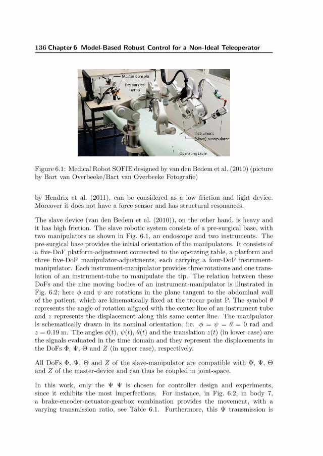
136 Chapter 6 Model-Based Robust Control for a Non-Ideal Teleoperator
Figure 6.1: Medical Robot SOFIE designed by van den Bedem et al. (2010) (pictureby Bart van Overbeeke/Bart van Overbeeke Fotografie)
by Hendrix et al. (2011), can be considered as a low friction and light device.Moreover it does not have a force sensor and has structural resonances.
The slave device (van den Bedem et al. (2010)), on the other hand, is heavy andit has high friction. The slave robotic system consists of a pre-surgical base, withtwo manipulators as shown in Fig. 6.1, an endoscope and two instruments. Thepre-surgical base provides the initial orientation of the manipulators. It consists ofa five-DoF platform-adjustment connected to the operating table, a platform andthree five-DoF manipulator-adjustments, each carrying a four-DoF instrument-manipulator. Each instrument-manipulator provides three rotations and one trans-lation of an instrument-tube to manipulate the tip. The relation between theseDoFs and the nine moving bodies of an instrument-manipulator is illustrated inFig. 6.2; here φ and ψ are rotations in the plane tangent to the abdominal wallof the patient, which are kinematically fixed at the trocar point P. The symbol θrepresents the angle of rotation aligned with the center line of an instrument-tubeand z represents the displacement along this same center line. The manipulatoris schematically drawn in its nominal orientation, i.e. φ = ψ = θ = 0 rad andz = 0.19 m. The angles φ(t), ψ(t), θ(t) and the translation z(t) (in lower case) arethe signals evaluated in the time domain and they represent the displacements inthe DoFs Φ, Ψ, Θ and Z (in upper case), respectively.
All DoFs Φ, Ψ, Θ and Z of the slave-manipulator are compatible with Φ, Ψ, Θand Z of the master-device and can thus be coupled in joint-space.
In this work, only the Ψ Ψ is chosen for controller design and experiments,since it exhibits the most imperfections. For instance, in Fig. 6.2, in body 7,a brake-encoder-actuator-gearbox combination provides the movement, with avarying transmission ratio, see Table 6.1. Furthermore, this Ψ transmission is

6.2 Model based robust control applied to SOFIE robot 137
Figure 6.2: Schematic Surgical Robot Sofie: joints and moving bodies. See van denBedem et al. (2010)
non-backdrivable, i.e. that it can only be moved from its actuation input. Morerelevant information and parameters of the instrument-manipulator are providedin Table 6.1. A real-time data acquisition (DAQ) system is used to couple the
Table 6.1: Tele-surgical system hardware parameters (van den Bedem et al.(2010)).
Friction Slave < 2.2 N mGearbox ratio slave-Ψ 1100− 1700 (varying)Force sensor Ψ:range 4 N m (20 N at the tipa)Force sensor Ψ:noise level < 6 mN m (< 0.03 N at the tipa)Friction master < 0.03 N mMaximum master torque fm 0.51 N mSampling frequency 4 kHz
a At nominal insertion depth z = 0.19 m

138 Chapter 6 Model-Based Robust Control for a Non-Ideal Teleoperator
101
102
−120
−100
−80
−60
−40
−20
Frequency [Hz]
Mag
nitu
de [
dB]
FRF Master MFRFΨ
(iω)
Fitted Model Master MΨ(iω)
FRF Slave SFRFΨ
(iω)
Fitted Model Slave SΨ(iω)
Figure 6.3: Magnitude of the Frequency Response Function (FRF) measurementsand magnitude bode diagram of the corresponding fitted models of Master andSlave Devices in Ψ DoF.
master and the slave robot. It consists of a dSPACE rack, running a Matlab-Simulink-generated real-time application with a sampling frequency of 4 kHz.
The magnitude of the Frequency Response Function (FRF) measurements from in-put torque (in N m) to output rotation (in rad) of the Ψ DoF is shown in Fig 6.3.In the same figure the respective magnitude bode diagram of the fitted modelsMΨ(iω) and SΨ(iω) for both master and slave devices are shown. During allexperiments in this work, all the other DoFs are kept at their nominal values.Hereafter, we assume the slave device interacts with the environment at the in-strument’s tip at a distance of LSE = 19cm from the trocar point P. In a similarway, we assume that the operator interacts at a distance of LMO = 20cm from therotation axes of Ψ in the master device. Therefore, for notational convenience, ifnot specified otherwise, when we use units of force, distance, mass, etc., we re-fer to those parameters computed on the interaction points previously described.Moreover, when we use units of torque, rotation, inertia, etc., we refer to thoseparameters computed either with respect to the trocar point P or to the master-
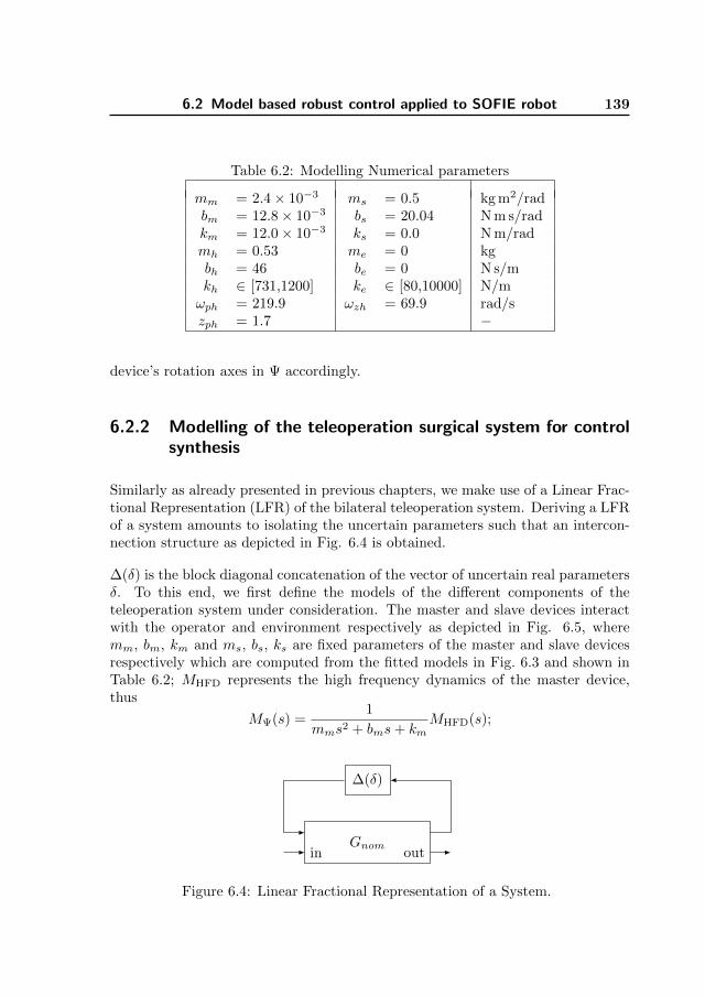
6.2 Model based robust control applied to SOFIE robot 139
Table 6.2: Modelling Numerical parameters
mm = 2.4× 10⁻³ ms = 0.5 kg m2/radbm = 12.8× 10⁻³ bs = 20.04 N m s/radkm = 12.0× 10⁻³ ks = 0.0 N m/radmh = 0.53 me = 0 kgbh = 46 be = 0 N s/mkh ∈ [731,1200] ke ∈ [80,10000] N/mωph = 219.9 ωzh = 69.9 rad/szph = 1.7 −
device’s rotation axes in Ψ accordingly.
6.2.2 Modelling of the teleoperation surgical system for controlsynthesis
Similarly as already presented in previous chapters, we make use of a Linear Frac-tional Representation (LFR) of the bilateral teleoperation system. Deriving a LFRof a system amounts to isolating the uncertain parameters such that an intercon-nection structure as depicted in Fig. 6.4 is obtained.
∆(δ) is the block diagonal concatenation of the vector of uncertain real parametersδ. To this end, we first define the models of the different components of theteleoperation system under consideration. The master and slave devices interactwith the operator and environment respectively as depicted in Fig. 6.5, wheremm, bm, km and ms, bs, ks are fixed parameters of the master and slave devicesrespectively which are computed from the fitted models in Fig. 6.3 and shown inTable 6.2; MHFD represents the high frequency dynamics of the master device,thus
MΨ(s) =1
mms2 + bms+ kmMHFD(s);
∆(δ)
Gnomin out
Figure 6.4: Linear Fractional Representation of a System.

140 Chapter 6 Model-Based Robust Control for a Non-Ideal Teleoperator
Operator
1
mms2 + bms+ kmMHFD
fm
fh
xm
(a)
Environment
1
mss2 + bss+ ks
fs
fe
xs
(b)
Figure 6.5: Diagram of (a) operator/master device and (b) environment/slavedevice.
fm, fs are the actuation forces to the master and slave devices respectively; fh, ferepresent the total force exerted by the operator and environment respectively; andxm, xs are the positions of the master and slave devices respectively, by definitionthey also represent the positions of the operator and environment respectively.Two main aspects of this application make the modelling different to the classicalteleoperation’s system modelling presented in literature. First, one can see thatthe dynamics of the master device have been split in a mass-damper-spring systemand high frequency dynamics. Such separation will be used to obtain the final LFRof the system. Second, the environment force is not fed-back to the slave device.This is a simplified model of the non-backdrivability property of the slave device.In practice, high loads on the instrument will lead to an increased friction on theslave device, which could be modelled and then friction compensation could beused, however, the focus is on testing the robust control technique under thosenon-ideal properties. The next step is to define models for both operator andenvironment.
Operator Model
For the operator, we make use of the model structure presented in Chapter 2 andshown in Eq. (6.2.2), in which it is assumed that the main source of uncertaintycomes from the operator’s arm-hand stiffness kh, which allows to reduce the controldesign complexity.
Zh(s) =Fh(s)
Xm(s)= (mhs
2 + bhs+ kh)Qh(s),

6.2 Model based robust control applied to SOFIE robot 141
where
Qh(s) =
s
ωzh+ 1
s2
ω2ph
+ 2zphs
ωph+ 1
.
We followed a similar procedure as proposed in Chapter 2. We performed differentexperiments to get FRF measurements Zmeas
h (jω) of Zh(s). Because the masterdevice does not have a force sensor, Zmeas
h (jω) is reconstructed using two FRFmeasurements. First we obtained an FRF from the closed loop from fm to xmshown in Fig 6.5.(a), i.e. the closed loop between the master device and theoperator’s hand. Then, MFRF
Ψ (iω) in Fig 6.3 is used to compute the operator’shand FRF Zmeas
h (jω).
We did three experiments in which we presented three virtual springs to theoperator with stiffness values in the range kVe ∈ [0, 5000] N/m such that fm =−kVe xm+f IDm , in which f IDm will be used as a disturbance signal for system identi-fication. In particular, we used a system’s sampling rate of 4000 Hz and a frequencyrange of [1, 40] Hz for the multi-sine. Initially we set f IDm = 0 N and then the op-erator was asked to move the master device in order to feel the virtual spring.Subsequently, the operator was asked to stop in a position of his/her choice wherehe/she could still feel the virtual spring. The idea is that the operator exerts aforce level such that he/she could feel that he/she has a correct haptic perceptionof the virtual environment. This is clearly subjective to the operator. Neverthe-less, the aim of the experiment is that the operator changes intuitively his/herexerted force and grip for different virtual springs. Afterwards, a multi-sine sig-nal was applied to the master device via f IDm while the operator tried to remainstatic. Actuation forces fm(t) and positions xm(t) were measured and then theirFourier transforms Fmeas
m (jω) = F(fm(t))(jω) and Xmeasm (jω) = F(xm(t))(jω)
were computed. Then, the frequency response function (FRF) measurements ofthe operator’s arm-hand dynamics Zmeas
h (jω) is computed in a frequency range of[1,20] Hz, the results of which are depicted in Fig. 6.6.
We observed that the quality of the obtained measurements is low especially above10 Hz. Nevertheless, the frequency content of the operator’s movement is assumedto be dominant in frequencies below that. Moreover, with the measurements weare interested mainly in obtaining a rough estimation on how the operator changeshis arm stiffness. As it will be shown on the experimental results, a model basedon this measurements is sufficient to obtain satisfactory results.
To reduce the complexity on the optimization process to fit the model parameters,we use the mass value mh found in Chapter 2 since it is assumed that the operatoruses a similar posture to manipulate the master device, i.e. with the elbow restedon a table, thus we use mh = 0.53 kg. Then, we optimized the variables bh, kh, ωzh,

142 Chapter 6 Model-Based Robust Control for a Non-Ideal Teleoperator
55
60
65
70
75M
agni
tude
[dB
]
100
101
0
45
90
135
Frequency [Hz]
Phas
e[de
g.]
MeasurementsLow freq. fits
Fits for kh, kh
Figure 6.6: Arm FRF Measurements in Ψ DoF.
zph and ωph to fit each measurement to the model minimizing the cost functionWZh
(iω) = ‖(Zh(iω) − Zmeash (iω))‖2 for ω ∈ 2π[1, 20] rad/s. The optimization is
done using a constrained nonlinear optimization method provided by the commandfmincon in Matlabr. Then, to reduce complexity of the model and the controldesign, we have used a low-frequency approximation by allowing variation in khonly and fixing all other parameters to their centred values of the correspondingintervals found in the optimization. Such fitted models are depicted in Fig. 6.6,where we used mh = 0.53 kg, bh = 46 N s/m, ωzh = 69.9 rad/s, zph = 1.7 andωph = 219.9 rad/s and kh = [877, 1000] N/m.
Finally, we include possible extra variation in kh to increase the robustness ofthe system. Hence, we enlarge the range of values of kh by 20% resulting in therange kh ∈ [731, 1200] N/m. The resulting Zh(s) fitted models for kh =731 N/mand kh =1200 N/m are shown with dashed lines in Fig. 6.6. All the operator’sparameters are summarized in Table 6.2. Though the identification was performedvia LTI techniques, in what follows below, we assume that during operation kh istime-varying within kh(t) ∈ [kh, kh] for all t > 0.
Combining the master device and operator models, we arrive at the model diagramfor the operator/master device depicted in the two upper blocks in Fig. 6.7, wheref∗h is the active force generated by the operator and ∆h = kh defines the time-varying, bounded and uncertain parameter of the human hand dynamics model.One can see that the master device model separation in a mass-damper-springsystem and high frequency dynamics allows for a representation such that a state

6.2 Model based robust control applied to SOFIE robot 143
1
s
1
s1mm
xmxmxm
mh
bh
kh
bm
km
f∗h
fh
fm
Master Device
Operator
−
−
MHFD
M−1Ψ = (mms
2 + bms+ km)LPF2−
LPF1
fh
−
Operator Force Estimator
Qh(s)
∆h
Figure 6.7: Block diagram representation of the operator/master device pair, andoperator force estimator.
space model can be easily extracted, which is necessary for control synthesis.
Operator’s force estimator
Next, for control synthesis it is desirable to have information about forces and po-sitions in both operator and environment sides. However, in real-life applications,the master device usually does not have a force sensor, as in the case here. To es-timate the operator’s force, in this work we implement a disturbance observer see,e.g., Schrijver and Van Dijk (2002), the structure of which is shown in the lowerpart of Fig. 6.7, where MΨ represents a model of the master device, LPF1 andLPF2 are low pass filters of first and second order respectively. In a standard im-plementation of a disturbance observer, an accurate model M is highly desirable.Moreover, the dashed interconnection in the lower part of Fig. 6.7 is used in anstandard observer to increase robustness of the estimated force accuracy againstmodel uncertainty. This results in the following mapping from the signals xm andfm to the estimate fh in a standard disturbance observer:
fh = (1− LPF1)−1LPF1(M−1Ψ xm − fm)

144 Chapter 6 Model-Based Robust Control for a Non-Ideal Teleoperator
We made two main modifications with respect to a standard disturbance observer.First, because we are interested in the operator’s force estimation only for lowfrequencies, and to decrease the order of the overall system model, in M−1
Ψ we useonly the low frequency part of the master device model, i.e. a mass-damper-springmodel structure, in which mm, bm and km are estimates of the mass, damperand stiffness of the master device, and in this case they only serve for illustrativepurposes since we do not know the real values, therefore we set them equal to thoseof the model from Fig 6.3. LPF2 is especially used to avoid a non-proper transferfunction, which does not have a state space representation, and also to avoidexcessive amplification of high frequency noise. Second, the dashed interconnectionin the lower part of Fig. 6.7 is usually used to increase the robustness propertiesof the estimator as previously mentioned. However, there is no guarantee that theobserver will be stable under such unitary feedback. Moreover, it can be seen as alocal force feed-back which will have effect on the haptic perception on the operatorside when combined with a controller, which will provide an additional loop fromfh to fm. Thus, to avoid those issues, we do not use the dashed interconnection.This results in the following mapping from the signals xm and fm to the estimatefh:
fh = LPF1(M−1Ψ xm − fm)
The loop from fh to fm is closed only via the controller, which will provide robustperformance of the overall system and guarantee stability properties of the forceobserver as will be shown in the results.
Environment model
Continuing with the system modelling, we consider environments with dominantspring dynamics:
fe = f∗e + kexs (6.1)
Here, ke ≥ 0 is the stiffness coefficient of the environment, and f∗e is the activeforce from the environment, if present. We focus on the environment stiffness keas the main cause of the environment dynamic variation, hence ke is assumed tobe bounded (though within a wide range), and time-varying, i.e ke(t) ∈ [ke, ke] forall t > 0. This choice is suitable for applications in which the effect of ke on feis dominant, e.g. in stiffness discrimination tasks like those in surgery. For otherenvironment types the uncertainty structure and parameters can be redefined.
In contrast to the master device, the slave device does have a force sensor whichprovides information on the environment force fe. Thus, the coupled environment/slave-device system can be obtain based on Eq. (6.1) and Fig. 6.5.(b). The uncer-tainty block in the environment/slave-device model is given, then, by ∆e = ke.
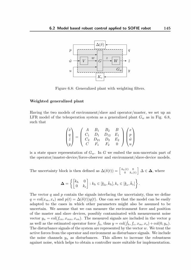
6.2 Model based robust control applied to SOFIE robot 145
G W
∆(δ)
V
Kc
w zw z
p
u
q
yGw
Figure 6.8: Generalized plant with weighting filters.
Weighted generalized plant
Having the two models of environment/slave and operator/master, we set up anLFR model of the teleoperation system as a generalized plant Gw as in Fig. 6.8,such that
xqzy
=
A B1 B2 BC1 D1 D12 E1
C2 D21 D2 E2
C F1 F2 0
xpwu
is a state space representation of Gw. In G we embed the non-uncertain part ofthe operator/master-device/force-observer and environment/slave-device models.
The uncertainty block is then defined as ∆(δ(t)) =[kh(t) 0
0 ke(t)
]∆ ∈∆, where
∆ =
{[kh 00 ke
]: kh ∈ [kh, kh], ke ∈ [ke, ke]
}.
The vector q and p contain the signals interfacing the uncertainty, thus we defineq = col(xm, xs) and p(t) = ∆(δ(t))q(t). One can see that the model can be easilyadapted to the cases in which other parameters might also be assumed to beuncertain. We assume that we can measure the environment force and positionof the master and slave devices, possibly contaminated with measurement noisevector yn = col(fen, xmn, xsn). The measured signals are included in the vector y
as well as the estimated operator force fh, thus y = col(fh, fe, xm, xs) + col(0, yn).The disturbance signals of the system are represented by the vector w. We treat theactive forces from the operator and environment as disturbance signals. We includethe noise channels yn as disturbances. This allows to increase the robustnessagainst noise, which helps to obtain a controller more suitable for implementation.
146 Chapter 6 Model-Based Robust Control for a Non-Ideal Teleoperator
Thus, we define w = col(f∗h , f∗e , fen, xmn, xsn). Additionally, the actuation signal
vector u is defined as u = col(fm, fs). Finally, the performance vector z is definedas z = col(fh − fe, xm − xs, fm, fs). Via the component fh − fe, we enforce thatthe human operator should feel the same force applied by the environment. Thesecond component, xm−xs, is the position error to obtain tracking between masterand slave. The actuation variables are also included as channels to be penalizedto avoid controllers with high gains. Finally, w and z are weighted copies of w andz via predefined filters V and W respectively, which allow to shape the desiredsystem performance.
The chosen performance criterion is defined as the L2 gain, γ, of the mappingfrom disturbance channels w to the performance channels z, as is customary inmodel-based H∞ control, e.g., see Skogestad and Postlethwaite (2005). The L2
gain from w to z can be expressed as:
sup06=w∈L2
||z||2||w||2
< γ, (6.2)
in which γ can be interpreted as a worst-case gain from the disturbances w to theperformance signals z. Therefore, instantaneous responses that can be felt by theoperator have a direct effect on the performance criterion. This makes the L2 gaina suitable performance criterion for teleoperation systems.
Finally, Kc represents the to-be-designed controller. The aim of the controllerdesign is then to find a controller Kc that has robust performance for all ∆ ∈ ∆.In the coming sections we will shortly describe the robust control methods to beevaluated in the surgical setup.
6.2.3 Robust control under time-varying uncertainties
One of the main objectives in this chapter is the evaluation of the model basedcontrol method for teleoperation proposed in Chapter 2. Such method allows tosynthesize a controller Kc such that the closed loop system in Fig. 6.8 has robustperformance under arbitrary fast and bounded parametric uncertainty given by∆ ∈ ∆. For the details on the exact control synthesis procedure, the reader isreferred to Chapter 2.
Such control design method has been satisfactorily tested in a one-DoF academicsetup with force and position sensors in both master and slave devices. In or-der to apply it to our specific application, all what we need is the model of oursystem, which was already obtained in Section 6.2.2, and the specification of theweighting filters W and V on the performance channels in Fig. 6.8, as it is cus-tomary in robust control design. With these filters we specify a desired level of
6.2 Model based robust control applied to SOFIE robot 147
force and position tracking in frequency domain. We use the same filter struc-ture as in Chapter 2, with the main modification that in our application we donot have force sensor at the master side. The filters V and W are block di-agonal transfer matrices emphasizing the frequency band in which we want theparticular channel to be penalized. Thus V = diag(Vf∗h , Vf∗e , Vfen , Vxmn , Vxsn) andW = diag(Wfh−fe ,Wxm−xs ,Wfm ,Wfs). Ideally, one wants to have fh−fe = 0 andxm−xs = 0. In this case we would get perfect transparency, but as is known, thistype of design is unrealistic (Lawrence (1993b)) and has poor stability properties.
Instead, it is desirable to relax such strict requirement, we are interested in forc-ing the force and position tracking errors such that in frequency domain |Fh(ω)−Fe(ω)| < |Fw(ω)| and |Xm(ω) −Xs(ω)| < |Xw(ω)| where Fw(ω) and Xw(ω) rep-resent the desired level of force and position tracking in the frequency band ofinterest. We use |Fw(ω)| > 0 and |Xw(ω)| > 0 sufficiently small at low frequenciesto achieve force and position tracking, which will lead to a desired level of perfor-mance in the frequency range in which the human operator performs movements.On the other hand, we need to have feasible control action that is magnitudebounded forces fm, fs and a reduced amplification at high frequencies, to avoidsaturation and the excitation of high frequency dynamics. Those requirements aretranslated into the filters W and V shaped accordingly. Thus we put more weightat frequencies where we want to lower the L2-gain.
After the filters have been defined, it is possible then to design a controller for aspecific range of bounded operator and environment stiffness.
6.2.4 Switching robust control via bumpless transfer of robustcontrollers
The methods in Section 6.2.3 can provide high robust performance for boundedenvironment stiffness ke in the range of low stiffness environments. However, inreal-life applications it might be desired to guarantee stability of the teleopera-tion system for a wide range of environment stiffness ke ∈ [ke, ke], covering alsostiff environments. In Chapter 3 it is shown that for those cases a single LTI con-troller might not be sufficient to achieve desired levels of robust performance of theteleoperation system, therefore the authors proposed a multi-controller structure,which will be tested in our non-ideal teleoperator. The main idea consists ofscheduling different robust controllers according to the estimate ke of the actualvalue of ke. Thus, a specific number Nc of LTI controllers are designed, in whichthe ith controller Kci(s) has an uncertainty set ∆i of robust performance, suchthat all regions combined form a larger set such that ∆ ⊆ ∆1 ∪ ... ∪∆Nc
, where∆ describes the uncertainty set of the system. Such uncertainty distribution is de-

148 Chapter 6 Model-Based Robust Control for a Non-Ideal Teleoperator
ke
... ...
kh
kei kei+1ke1 keNc = kekei+1keike1 = ke keNc
kh
kh ∆1 ∆i ∆i+1 ∆Nc
Figure 6.9: Uncertainty regions ∆i of a switching robust controller.
picted in Fig. 6.9. The overlap between regions can be used to guarantee stabilityunder bounded uncertainty in the estimation signal ke.
Next, in order to switch between controllers in a stable way, in Chapter 5 we usedbumpless transfer of robust controllers, which is an extension of the bumplesstransfer technique by Zaccarian and Teel (2005). The main idea is to keep allcontrollers online, either with the real plant, or with a virtual model. This ideais illustrated in Fig. 6.10, where Kci represents the controller that is currentlyactive, and Kcj one of all the other Nc − 1 controllers that remain disconnected
Master-Slave DevicesHuman OperatorEinvironment
Bumpless Compensator forKci
−
Kci −
−Kcj
...
Bumpless Compensator forKcj
∆Bj =
[kBh 00 kBej
]
Gpzy
qwu
~0
−
u y
Figure 6.10: Bumpless Transfer Scheme for Teleoperation Control

6.2 Model based robust control applied to SOFIE robot 149
from the real system. The bumpless compensator for Kcj consists then by a plantout of the corresponding group of plants for which the controller is robust to.Therefore we used the same model G as in Fig. 6.8 but we select a single element
∆ = ∆Bj =
[kBh 00 kBej
]from the corresponding region ∆j . In this way the off-
line controller is virtually kept on-line and since we used ∆Bj ∈ ∆j , its stability,
while off-line, is guaranteed.
This technique has been experimentally tested in a one-DoF setup in Chapter 5,and will be evaluated in our surgical system.
6.2.5 Environment estimation
To be able to implement the multi-controller structure, we need an estimator thatis able to deal with abrupt changes of the environment stiffness ke. We makeuse of the same estimator as in Chapter 3, which is an estimator proposed inGustafsson (2000). The structure of the estimator is shown in Fig. 6.11. Theworking principle of this estimator is as follows: the filter block processes thediscrete inputs uk and outputs yk of a system described by a model (in our case an
environment model) to get an estimate θk of certain parameters θk (the parametersof our environment model). Then, the signal εk is used to detect abrupt changesin the parameters and under certain criteria, the detector block sends an alarm tothe filter to adapt quickly to the changes. Following the guidelines in Gustafsson(2000), the different blocks are described below.
Environment model as a linear regression model
We write our environment model in the following form
yk = ϕTk θk + ek
where k denotes sampled time instants, yk is the measured environment force, ek isthe corresponding noise, the environment parameters vector is θk = col(ke(k), f∗e (k))with f∗e (k) being the active component of the environment force, and the so called
Figure 6.11: Estimator with Change Detection

150 Chapter 6 Model-Based Robust Control for a Non-Ideal Teleoperator
regression vector ϕk is given by ϕk = col(uk, 1) with uk = xs(k) being the positionof the slave device.
Filter
For the filter block we utilize a Kalman filter for linear regressions, which is im-plemented in its recursive form as follows:
ϕk = col(uk, 1)
Kk =Pk−1ϕk
Rk + ϕTk Pk−1ϕk
Pk = Pk−1 −Pk−1ϕkϕ
Tk Pk−1
Rk + ϕTk Pk−1ϕk+Qk
θk = θk−1 +Kk(yk − ϕTk θk−1)
εk = yk − ϕTk θkwhere θk is the estimated vector of the environment model parameters, Rk is takenas 1 without loss of generality and Qk is a design parameter that determines thespeed of converge of the filter. Large values of Qk make the filter to react fasterbut also the estimate will have more noise. The variable εk is the error betweenthe actual measurement and the reconstructed measurement obtained with θk.
Detector
The detector block is defined as a threshold function in order to decide when tomake the filter to react fast. Thus, when |εk| < L|εk|, no alarm is generated and weuse Qk = Qnom. When |εk| ≥ L|εk|, it means that yk has deviated too much fromthe true measurement and the filter must adapt rapidly to the new environmentby setting Qk = Qfast.
Therefore, the estimator is tuned via L|εk|, Qnom and Qfast. This tuning is es-sential to be able to detect abrupt changes fast enough to schedule on time thecontrollers of the multi-controller structure.
6.3 Results of robust control applied on SOFIE robot
In this section we provide synthesis, simulations and experimental results. Initiallyone robust controller designed with the method mentioned on Section 6.2.3 is

6.3 Results of robust control applied on SOFIE robot 151
evaluated on the surgical system. Then, a multi-controller structure as describedin Section 6.2.4 is also implemented and experimentally tested.
6.3.1 Controller synthesis results
For the controller synthesis we tune the weighting filters such that force and po-sition tracking is achieved for frequencies below fbw = 10 Hz, and the actuationforces fm, fs are penalized from 60 Hz and beyond. The reader is referred toChapter 2 for more details on the weights structure and fine tuning procedure.Moreover, the cut-off frequency of the low pass filters LPF1 and LPF2 in the forceestimator is set to 20 Hz, which suppress noise above the frequencies of interest.
For the first controller to be evaluated, we select a desired environment rangeas ke ∈ [80, 3000] N/m, which covers the range of stiffness present in soft tissueenvironments (see Gerovich et al. (2004)).
Then, using the model found in Section 6.2.2, we apply the control synthesisprocedure of Chapter 2. We get a controller Kc(s) covering the uncertainty regionof interest and with a performance index γ = 10.7. The resulting order of thecontroller OKc
= 21, which is equal to the order of the generalized plant Gw, i.e.including the weighting filters. We make the remark that in comparison to classicalcontroller schemes like position-position error, position-force, etc., the obtainedcontroller does not have a defined structure, other than its number of inputs andoutputs. In that sense the controller uses all available combinations from inputs tooutputs, as opposed to most classical controller architectures in which some input-output combinations are not used. Hereafter, the obtained Robust Controller (RC)will be referred as the RC.
Next, for illustrative purposes, we evaluate the properties of the force estimatorwhen used in combination with the RC. We added uncertainty in the model used inthe estimator by setting its parameters to mm = cpmm, bm = cpbm and km = cpkmfor cp ∈ [0.8, 1.2]. Then, we computed the transfer functions from fh to fh. Wecompare two cases, in the first one, we used the standard dashed interconnectionin Fig. 6.7, in the second one, instead, we used the control element from fh tofm of the RC previously designed. The magnitude bode diagrams of the resultingtransfer functions from fh to fh are depicted in Fig. 6.12. As reported in theliterature, the standard feedback provides robust and accurate estimations in thefrequency region of interest. However, from the figure one can see resonance peaksthat can have undesirable effects on the haptic feedback to the operator. On topof that, the estimator is not to be stable for cp ∈ [0.8, 0.9]. On the other hand,the estimator using the feedback via Kc(s) presents better stability robustnessproperties because all transfer functions were stable. Moreover resonance peaks

152 Chapter 6 Model-Based Robust Control for a Non-Ideal Teleoperator
10−1
100
101
102
−50
−40
−30
−20
−10
0
10
20
30
Frequency [Hz]
Mag
nitu
de [
dB]
fh
fhstandard feedback
fh
fhfeedback via Kc(s)
Figure 6.12: Magnitude Bode Diagram of the transfer functions from fh to fhunder model uncertainty; using a standard feedback loop and a feedback via therobust controller Kc(s)
are not present which is beneficial for our application. As a trade-off, robustnessof the estimation accuracy is slightly degraded for very low frequencies, which didnot have a significant influence on the simulation and experimental phase as willbe shown later.
Next, we also evaluate a multi-controller based on bumpless transfer of robustcontrollers. The controller designed based on this structure is hereafter referredas the Bumpless Transfer Controller (BTC). For this controller, we select a widerrange of environment stiffness ke ∈ [80, 10000] N/m. We divide the total un-certainty region in two partitions, therefore Nc = 2. We select the first regionequal to the previous synthesis case covering soft tissue environments, i.e. ∆1 ={[
kh 00 ke1
]: kh ∈ [731, 1200], ke1 ∈ [80, 3000] N/m
}. Thus we can use the controller
Kc(s) as Kc1(s). For the second region we select ∆2 ={[
kh 00 ke2
]: kh ∈ [731, 1200],
ke1 ∈ [2500, 10000] N/m}. After applying the synthesis procedure inChapter 2, weget a controller Kc2(s) with a performance index γ = 9.2. Both controllers Kc1(s)and Kc2(s) have an order of OKc1
= OKc2= 21.
In order to improve the operator’s haptic perception when the slave device is in“free air”, i.e. no contact with any environment, we implemented a PID controller(with a weak integrator and additional low-pass filters) that tracks the position ofthe master device in the slave device. The idea is that this controller is only activewhen the environment force is lower than a small threshold fe < 0.05 N m. Thus,the operator will only feel the dynamics of the light master device. We defined
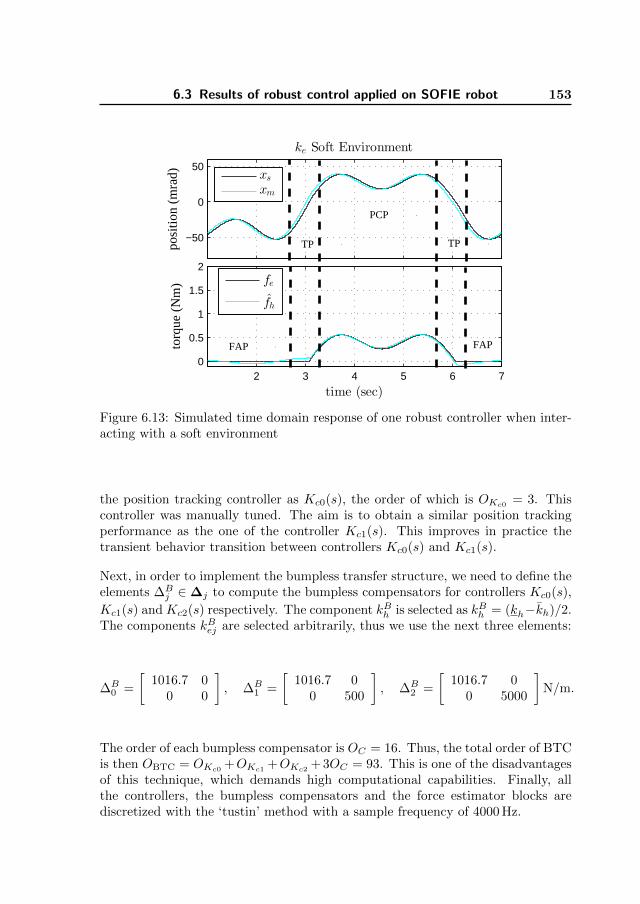
6.3 Results of robust control applied on SOFIE robot 153
−50
0
50
ke Soft Environment
posi
tion
(mra
d)
xsxm
2 3 4 5 6 70
0.5
1
1.5
2
torq
ue (
Nm
)
time (sec)
fe
fh
TP
PCP
TP
FAP FAP
Figure 6.13: Simulated time domain response of one robust controller when inter-acting with a soft environment
the position tracking controller as Kc0(s), the order of which is OKc0 = 3. Thiscontroller was manually tuned. The aim is to obtain a similar position trackingperformance as the one of the controller Kc1(s). This improves in practice thetransient behavior transition between controllers Kc0(s) and Kc1(s).
Next, in order to implement the bumpless transfer structure, we need to define theelements ∆B
j ∈∆j to compute the bumpless compensators for controllers Kc0(s),
Kc1(s) and Kc2(s) respectively. The component kBh is selected as kBh = (kh−kh)/2.The components kBej are selected arbitrarily, thus we use the next three elements:
∆B0 =
[1016.7 0
0 0
], ∆B
1 =
[1016.7 0
0 500
], ∆B
2 =
[1016.7 0
0 5000
]N/m.
The order of each bumpless compensator is OC = 16. Thus, the total order of BTCis then OBTC = OKc0
+OKc1+OKc2
+ 3OC = 93. This is one of the disadvantagesof this technique, which demands high computational capabilities. Finally, allthe controllers, the bumpless compensators and the force estimator blocks arediscretized with the ‘tustin’ method with a sample frequency of 4000 Hz.

154 Chapter 6 Model-Based Robust Control for a Non-Ideal Teleoperator
6.3.2 Simulation results
To test the controllers, we simulate a scenario in which an operator manipulatesthe system with the slave device in free-air and then gets in contact with a springlocated at xs > 0. Then after some periodic movements the operator comes backagain to the slave in the free-air situation. As an example of such scenario seeFig. 6.13. The Free Air Parts (FAP) correspond to time slots when there is nocontact with the environment. The Transient Parts (TP) correspond to time slotswhere there is a transition between the FAP and contact with the spring or vice-versa. The Permanent Contact Part (PCP) is a time slot after the TP has passedand periodic movements are performed while being in permanent contact withthe spring. For the opertaor we have used f∗h = (2 cos(1/3πt) + cos(πt))N m and
kh = 1016.7 N/m. In the simulations, both signals fh and fh have unnoticeable
differences in the plots, therefore we only plot the signal fh when we illustratethe operator force, this to be consistent with the experiments in which the realoperator force is not available.
First, we test the Robust Controller (RC). We simulate the closed-loop systeminteracting with a spring with ke = 400 N/m, which represents a soft environment.The corresponding time domain response of the position and force signals arepresented in Fig. 6.13. One can see stable responses during the Transient Parts(TP), which is ensured from the synthesis of the RC. Moreover we observe thatin the Permanent Contact Part (PCP) there is force and position tracking of thesimulated teleoperated system. On the other hand, the force tracking degradesduring the Free Air Parts (FAP) and some forces are noticeable in the operator side,These forces can degrade the haptic rendering of a free-air environment providedby the teleoperator.
Next, we test the Bumpless Transfer Controller (BTC) by simulating the closed-loop system with springs with ke = 400 N/m and ke = 10 000 N/m representingsoft and stiff materials respectively. For simulation purposes we assume we canknow perfectly the environment stiffness, thus we set ke = ke. The time domainresults are depicted in Fig. 6.14, on the left for the soft spring, and on the rightfor the stiff environment.
One can see that the response in the FAPs is improved because now fh is closeto zero in those time slots. For the soft spring, we can see that during the TP,the transient response is smooth and barely noticeable, despite the fact that thereis a switch between Kc0(s) and Kc1(s). Next, regarding the interaction with thestiff spring, the response presents some overshoot behavior during the TP, yetthat overshoot in positions and forces is rapidly damped out. During the PCP, forthe soft spring force and position tracking is obtained as expected from the RCresults. For the stiff spring, we can see that the position tracking degrades slightly,

6.3 Results of robust control applied on SOFIE robot 155
−50
0
50
ke Soft Environment
posi
tion
(mra
d)
0
1
2
torq
ue (
Nm
)
0
5
10
stiffness(103N/m)
2 4 60
1
2
activeK
i
time (sec)
ke Stiff Environment
xsxm
fe
fh
ke
14 16 18
time (sec)
Figure 6.14: Simulated time domain response of bumpless transfer controller wheninteracting with an environment with stiffness ke = 400N/m (left) and ke =10000N/m (right).
however the operator still would perceive a correct haptic perception of the stiffenvironment as it will be shown later.
We also analyse the performance of the system by means of force versus positionplots on the environment and operator sides as shown in Fig. 6.15. The slopeof fe versus xs plots represent the stiffness of environment and the slope of thefh versus xm plots represent the stiffness being felt by the operator. We cansee that in the PCP both controllers Kc1(s) and Kc2(s) provide to the operatora haptic perception close to that of the environment, which is desirable in ourapplication. Moreover, during the FAP the estimated operator’s force is verysmall, which is desirable when there is not environment in contact with the slavedevice. These simulations results confirms that the controller design through theproposed methods leads to promising results. In the next section we present results

156 Chapter 6 Model-Based Robust Control for a Non-Ideal Teleoperator
−50 0 50
0
0.5
1
1.5
2 ke Soft Environmenttorque(N
m)
position (mrad)
Environment
Operator
−50 0 50
ke Stiff Environment
position (mrad)
Figure 6.15: Simulated time domain response of one robust controller when inter-acting with an environment with stiffness ke = 400N/m (left) and ke = 10000N/m(right).
of both controllers, the RC and the BTC, that validate experimentally the usedcontrol design methodology.
6.3.3 Experiments
In this section, we validate the RC and the BTC with experiments on the surgicalsetup described in Section 6.2.1.
We test two different environments: a soft foam with stiffness ke≈ 400 N/m, and astiff foam with ke≈ 10 000 N/m. For the experiments, we drove the system undersimilar operating conditions as to the simulation part, i.e. Free-Air Parts
Initially we test the RC controller, the time domain responses for the interactionwith both type of environments are depicted in Fig. 6.16. Regarding the interactionwith the soft foam, the response during the TPs is completely smooth, i.e. thereare neither oscillations nor overshoots, which verifies the robustness properties ofthe RC controller. During the PCP, the tracking performance is less than that ofthe simulations results, which can be mainly due to the high friction present in theslave device. However, if we analyse the results by means of force versus positionplots as depicted in Fig. 6.17, one can see that in the PCP the operator perceivesa similar stiffness as that of the environment, which validates the potential of thecontrol approach. Next, the interaction of the RC with a stiff environment resultedin an unstable behaviour as can be seen from the oscillations in Fig. 6.16, resultwhich could be already expected from the controller synthesis, because robust

6.3 Results of robust control applied on SOFIE robot 157
−150
−100
−50
0
50
ke Soft Foam
posi
tion
(mra
d)
10 12 14
0
0.5
1
torq
ue (
Nm
)
time (sec)
ke Stiff Foam
xsxm
9 10 11 12 13time (sec)
fe
fh
Figure 6.16: Time domain response of one robust controller when interacting withdifferent environments
performance is not guaranteed for stiff environments. (FAP), Transient Parts(TP) and Permanent Contact Part (PCP).
Regarding the FAPs one can see some noticeable forces on the operator side which
−150 −100 −50 0 50−0.2
−0.1
0
0.1
0.2
0.3
0.4
0.5ke Soft Foam
torque(N
m)
position (mrad)
Environment
Operator
Figure 6.17: Force versus Position plots from experiments of a robust controllerwhen there is interaction with a soft foam.
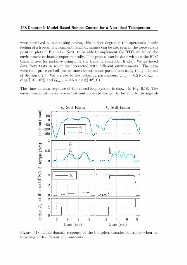
158 Chapter 6 Model-Based Robust Control for a Non-Ideal Teleoperator
were perceived as a damping action, this in fact degraded the operator’s hapticfeeling of a free-air environment. Such dynamics can be also seen in the force versusposition plots in Fig. 6.17. Next, to be able to implement the BTC, we tuned theenvironment estimator experimentally. This process can be done without the BTCbeing active, for instance using only the tracking controller Kc0(s). We gathereddata from tests in which we interacted with different environments. The datawere then processed off-line to tune the estimator parameters using the guidelinesof Section 6.2.5. We arrived to the following parameters: L|εk| = 0.2 N, Qfast =diag([106, 103]) and Qnom = 0.5× diag([102, 1]).
The time domain response of the closed-loop system is shown in Fig. 6.18. Theenvironment estimator works fast and accurate enough to be able to distinguish
−150−100
−500
50
ke Soft Foam
posi
tion
(mra
d)
0
0.5
1
torq
ue (
Nm
)
0
2
4
stiffness(103N/m)
6 7 8 90
1
2
activeK
i
time (sec)
ke Stiff Foam
xsxm
fe
fh
ke
2 4 6 8
time (sec)
Figure 6.18: Time domain response of the bumpless transfer controller when in-teracting with different environments.

6.3 Results of robust control applied on SOFIE robot 159
−150−100 −50 0 50−0.2
0
0.2
0.4
0.6
0.8ke Soft Foam
torque(N
m)
position (mrad)
EnvironmentOperator
−150−100 −50 0 50
ke Stiff Foam
position (mrad)
Figure 6.19: Time domain response of the switching robust controller when inter-acting with different environments
between the two types of environments. We make emphasis that a correct tuningof the estimator is important, this because a fast detection in the changes allowsto schedule the controllers on time, accuracy is only important to determine theregion in which the stiffness environment lies and not its exact value.
Next, when interacting with the soft spring, the responses in the TPs are freeof overshoots and oscillations and the results are very similar as those in thesimulations. Moreover, the FAP is improved with respect to the RC. In fact inthis scheme the operator does not feel additional dynamics other than those of themaster device, and because it is light, the haptic perception of having a free-airenvironment on the slave side is realistic. To have a different picture of the results,forces versus position plots for this test are presented in the left part of Fig. 6.19.One can see that the BTC provides a very similar stiffness of the environment at theoperator side at all times. The response during the TP when getting into contactwith a stiff environment presents some overshoot, however the stability was notcompromised during the experiments. Subsequently, during the PCP, the operatorperforms periodic movements, however the slave does not move during this timeslot. The cause for the lack of movement of the slave device in stiff environmentscomes from two combined facts: first the slave device is non-backdrivable, whichin principle means that the device only moves when it actuated from the actuationsignals fs, second, the slave device has high friction, thus, the actuation signalsfrom the controller need to be sufficiently large to move the slave device. Yet withthis phenomenon, the operator was able to perceive a high stiffness on the masterside as can be in Fig. 6.19.
160 Chapter 6 Model-Based Robust Control for a Non-Ideal Teleoperator
6.3.4 Discussion
The simulation and experimental results for the RC confirmed the results obtainedin Chapter 2. The description of the operator and environment as explicitly time-varying is suitable for the controller synthesis in bilateral teleoperation, especiallybecause of the sudden changes in the environment. Moreover, because we useda model based control synthesis, there are no restrictions on matches in the me-chanical properties of the master and slave devices to apply the method, contraryto for instance in Willaert et al. (2014). The main challenge in this chapter wasto apply the synthesis methods in an non-ideal teleoperator with properties likethe non-backdrivability of the slave device and not having a force sensor in themaster device. The latter aspect was challenging in order to get a model for theoperator. Nonetheless, it was enough to get a rough estimation of the operator’smodel parameters in order to obtain good experimental results, which shows thateven under those limitations the synthesis method can be applied.
Moreover, the fact that we included the force estimator in the system’s model, wasessential to obtain good experimental results. The standard disturbance observercan have poor stability robustness properties as found before. In our case, theloop from fh to fm was designed only by the control synthesis procedure, thus itwas guaranteed that a stable force estimator is obtained. Moreover its stabilityrobustness properties against model uncertainty were improved.
Next, regarding the multi-controller structure, the results showed that multiplecontrollers, which were designed to have a good performance in their respectiveregions of interest of environment stiffness, were successfully combined by means ofthe bumpless transfer technique proposed in Chapter 5. Thus the operator couldhave a good feeling when the slave is in free air, plus a good stiffness reflectionwhen discriminating soft tissues and, additionally, a feeling of a high stiffness forstiff environments, all this combined while having a stable interaction. In fact, theswitching between the controller Kc0(s) and Kc1(s) is made in a stable and smoothway, which makes the BTC very promising in applications where it is expectedthat the slave device is mainly either on free-air or in contact with soft tissue. Theswitch to controller Kc2(s) presents some overshoot behavior but stability was notcompromised during the experiments. The subsequent force and position trackingwas degraded but still a high stiffness is provided to the operator. However, ifforce tracking under stiff environments is relevant, for instance for cutting bone,then such an issue needs improvement. This may be achieved by implementingfriction compensation on the slave device.
Finally, during the experimental phase we noticed that the accuracy of the envi-ronment estimator degrades for high values of stiffness, e.g. ke> 4000 N/m, theestimated values did not increased much despite the stiff environment. One of

6.4 Conclusions 161
the reasons we found is that the slave device barely moves right after getting incontact with the stiff environment due to the non-backdribality and high frictionof the slave device. In terms of the parameter estimation it means that no newinformation is available to update further the estimations. This behaviour wouldbe problematic for techniques that rely on an accurate environment estimator, e.g.Willaert et al. (2010), Cho et al. (2013). In the BTC structure estimator accuracyis needed only around the overlapping region between ∆1 and ∆2, which is usedto determine whether to use Kc1(s) or Kc2(s). Thus, the BTC offers an advantagein that respect with other techniques that use environment estimation parametersin their control laws, and rely more on parameter estimation accuracy in a widerange of environment stiffness.
6.4 Conclusions
In this chapter we have implemented two type of controllers in a tele-surgical setup:one with a single LTI controller, and one with a multiple-controller structure. Bothtypes were designed with model based robust control techniques. Because there isno sensor at the master device, rough estimates of the operator’s model parame-ters were computed. Even with this limitation, the obtained experimental resultsmatched with the theory and simulations. Moreover, due to the lack of force sensorin the master device, a disturbance observer was implemented to obtain an esti-mate of the operator’s force. Despite the possible mismatch between the model ofthe master device and the real device, analysis showed that the proposed imple-mentation of the operator’s force estimator delivers accurate and robust estimates.Such result was obtained because the disturbance observer model was included inthe system’s model, improving the stability properties of the estimator after thecontrol synthesis. Additionally, the results showed that it is possible to combinemultiple robust controllers to reflect to the operator, in a stable way, a stiffnesssimilar to that of the environment. Moreover, satisfactory results were obtainedfor different types of environment, ranging from free air and soft to stiff environ-ments, despite non ideal properties of the surgical setup, like non-backdrivability,high mass and high friction in the slave device, and lack of force sensor on themaster device. All this demonstrates the suitability and potential of the utilizedcontrol methods to be implemented in real-life engineering practice.

162

163
Chapter 7
Conclusions andRecommendations
7.1 Conclusions
In this thesis, we have presented a systematic approach towards control design forbilateral teleoperation. The approach involves modelling of the teleoperation sys-tem, in which we use models of the operator derived from experiments, and we usepre-defined models of the environment motivated by the type of the applicationsconsidered. In this way, the set of uncertain dynamics of the bilateral teleoperationsystem can be narrowed down to those present in a particular application, thus al-ready reducing the conservatism in the modelling phase. Moreover, the proposedmodel describes the uncertain dynamics by means of parametric uncertainties.This allowed us to handle the uncertain parameters of the bilateral system in asystematic way. Therefore, it was possible to take explicitly into account proper-ties like boundedness and time-variation of the operator and environment modelparameters during control design.
Based on this modelling, we used synthesis tools that allowed us to systematicallyand simultaneously address stability and performance, in contrast with conven-tional methods in which both are treated separately. Throughout this thesis, theanalysis, simulation and experimental results of the cases at hand were consis-tent with each other, showing that the assumptions we made during modellingand synthesis were appropriate, thus demonstrating the potential of the designmethodology here presented. In this thesis we used a performance criterion basedon force and position tracking. The synthesis tools allow for other performance

164 Chapter 7 Conclusions and Recommendations
1000 1000020
40
60
80
100
ke [N/m]
kro(%
)
RCSRCWSRCCL
SRCDT
Figure 7.1: Orthogonal linear regression analysis results to evaluate stiffness reflec-tion in the simulations. kro(%) is the percentage of the environment stiffness that isreflected to the operator is shown. RCS: Robust Controller for Soft environmentstiffness (Chapter 2). RCW: Robust Controller for Wide range of environmentstiffness (Chapters 3 and 4). SRCCL: Switching Robust Controller with CommonLyapunov Function (Chapters 3 and 4). SRCDT: Switching Robust Controllerwith Dwell Time conditions (Chapter 4).
criteria as long as they can be represented as linear matrix inequalities.
In order to quantify and compare the results obtained with the different techniquesproposed in this thesis, we performed an analysis to determine the percentage kroof environment stiffness that is reflected to the operator. The analysis is the sameas the one performed in Chapter 3. We took the responses in time domain of thesystem and extracted the data from the time slots in which there is a permanentcontact with the environment. Then, for each set of data of forces versus positionsvalues, an orthogonal regression is applied in order to fit a straight line. The slopeof such a line is an estimation of the stiffness value corresponding to the respectiveset of points of force versus position values. The orthogonal regression uses the sumof the squares of the distance of the data points to the fitted line as optimizationcost. This procedure is applied to both the operator and the environment sides.The ratio between both yields the percentage kro of environment stiffness that isreflected to the operator. The analysis is performed for all controllers that weredesigned for the 1-DoF setup utilized in this thesis. The results of the analysis forall the simulations is presented in Fig. 7.1 and the results of the analysis for allthe experiments is illustrated in Fig. 7.2.

7.1 Conclusions 165
1000 10000 10000020
40
60
80
100
ke [N/m]
kro(%
)
RCSSRCCL
BTC
Figure 7.2: Orthogonal linear regression analysis results to evaluate stiffness re-flection in the experiments. kro(%) is the percentage of the environment stiffnessthat is reflected to the operator is shown. RCS: Robust Controller for Soft environ-ment stiffness (Chapter 2). SRCCL: Switching Robust Controller with CommonLyapunov Function (Chapter 3). BTC: Bumpless Transfer Controller (Chapter 5).
Regarding the specific design case when a single robust controller is used, fromFigures 7.1 and 7.2 one can see that kro is always greater than 90%. Hence,the simulation and experimental results demonstrated that the proposed methodsallowed to obtain high performance and stability simultaneously in the range ofsoft environments, not only during continued contact, but also for sudden changesof the environment as observed in the time domains plots. This confirms thatby treating explicitly the operator and environment model parameters as time-varying, the bilateral teleoperation system is described more realistically. FromFig. 7.1 one can see that if a single robust controller is designed for a wide range ofvalues of environment stiffness, the overall factor kro decreases, which is an exampleof the robust stability and performance trade-off in bilateral teleoperation systems.
In order to improve the performance of the system and to extend the usable rangeof values of environment stiffness, in this thesis we have also proposed a multi-controller structure. The main idea is that several robust controllers are scheduledaccording to an estimate ke of the actual environment stiffness. The main challengeof this type of control is to achieve a stable and preferably smooth transitionbetween the different controllers, especially because in bilateral teleoperation largeovershoots and oscillatory behavior responses can degrade the haptic perceptionof the operator. To this end, we explored three different methods for controllerswitching, one based on the existence of a common lyapunov function, one basedon dwell time conditions, and one based on bumpless transfer.

166 Chapter 7 Conclusions and Recommendations
Even under the requirement on the existence of a common lyapunov function,the synthesis results showed that it is possible to improve the performance ofthe teleoperated system using the multi-controller structure, in comparison withthe case when only a single LTI robust controller is used. Analysis results ofkro in Fig. 7.1 confirm such overall improvement of performance. Moreover, thesimulations and experiments validated the synthesis results and also demonstratedthat indeed a smooth and stable switching among controllers is achieved becausethey all share a common lyapunov function.
In the case in which the controller synthesis was based on dwell time conditions, thetheoretical results demonstrated that the flexibility added on the relation betweenthe lyapunov functions corresponding to the different controllers indeed resultedin improved performance. This is confirmed by a better overall kro with respect tothe other controllers evaluated in Fig. 7.1. Although the simulation showed thatswitching is made in a stable way, stability is only guaranteed under the conditionthat the dwell times are respected. However, smoothness during switching is notfully guaranteed, for instance, if a large dwell time is used during synthesis, theresults would be equivalent to having all the controllers designed independently,for which a direct switch would cause oscillatory dynamics and large overshootswhich compromises the system’s stability. Hence, more insight is needed in therestrictions on the usable average dwell times that can work on practice.
Interestingly, even if the controllers are designed independently, experimental re-sults showed that stable switching among the controllers can still be achieved usingthe proposed bumpless transfer scheme. The main advantage of this scheme is thateach controller can be separately optimized for performance in its correspondingregion of uncertainty dynamics. The analysis results in Fig. 7.2 shows that anoverall improved kro is achieved with the proposed scheme. In conclusion, it waspossible to successfully combine one controller optimized for low and mediumstiffness values and another optimized for stiff environments, thus improving theoverall performance of the system.
The stability of the multi-controller schemes depends on the fast convergence ofthe environment estimator. However we point out that the accuracy is neededonly to determine to which region the environment stiffness belongs to. Thusthe estimator can be optimized for this purpose. In fact, we showed that it ispossible to implement an estimator that has a fast response to sudden and rapidchanges in the environment. The corresponding response time was small enough toperform stable switching among the LTI controllers of the multi-controller schemes.However, more insight is needed to know what is the maximum allowable estimatorresponse time to guarantee stability of the closed loop system. On the other hand,a parameter estimator is not per se needed to determine which controller shouldbe active, because it is only needed to know to which region the environment

7.1 Conclusions 167
currently belongs. Alternatives approaches are suggested in the next section.
Throughout this thesis we proposed different control design methodologies, sys-tematically increasing the performance of the bilateral teleoperation system asconfirmed by the analysis of the simulation and experimental results in Figures 7.1and 7.2 respectively. Comparing the multi-controller structures, one can see theimprovement was mainly noticeable for low environment stiffness, which is theregion of environment stiffness of major interest in many medical applications.
The model-based robust control approach was implemented in a real telesurgicalsetup. Because there was no force sensor at the master device, we made use of adisturbance observer to obtain an estimate of the operator’s force. A key aspectto a successful implementation was the fact that the disturbance estimator wasincluded in the model together with the master device and operator dynamics.In this way, the controller synthesis guaranteed the stability of the whole systemincluding the estimator. Moreover, analysis results showed that the proposedimplementation of the operator’s force estimator delivers robust estimations. Theexperimental results demonstrated that the model-based robust control is alsosuitable for non-ideal teleoperators, with characteristics such as a heavy, non-backdrivable slave and a master device with structural resonances and no forcesensor. This shows the suitability and potential of the utilized control methods tobe implemented in real-life engineering practice.
Regarding numerical complexity of the different methods, there are two aspects tolook at, the synthesis complexity and the implementation complexity. In terms ofsynthesis complexity, for the single robust controller case, the number of variablesto be solved by the LMI depends directly on the order of the models and thenumber of uncertain parameters of the system. In the multi-controller case, thesynthesis complexity increases proportionally with the number of LTI controllersto be used because all the controllers have to be designed simultaneously. Incontrast, the bumpless transfer scheme allows for independent controller design,which allows to split the synthesis complexity in parts. On the other hand, interms of implementation complexity, the bumpless transfer exhibits the worse casebecause all the controllers need to be active either in the loop with the real plant orin a virtual loop with a plant model, which is the main disadvantage of this scheme.The other schemes require less computational power since only one controller isactive at a time.

168 Chapter 7 Conclusions and Recommendations
7.2 Recommendations for future research
The methods and results presented in this thesis are just a preamble to show thepotential of the proposed approach, and it opens a new research line on modellingand control design for bilateral teleoperation systems. There are still several openchallenges in order to develop further the methodologies here presented. Thus, inthis section we indicate the main points for improvement and give future directionsto continue this research in different areas.
ModellingIn this thesis, the human arm models were derived from experiments conductedon one operator and for specific types of posture, while he/she grabbed the mas-ter devices. Thus, it is desirable to broaden te model to cover different posturesand operators. It is expected that the group of muscles that an operator useswhile manipulating the master device will change for different postures. Thus,we foresee this will increase the range of variation of parameters like mass anddamping of the model found in Chapter 2, thus more parameters would need tobe considered uncertain as well. This will increase the set of dynamics covered,however, the utilized methods in this thesis describe arbitrary fast time-varyingparametric uncertainty, which might be too conservative, limiting the achievableperformance. Therefore, increasing the number of uncertain parameters should becomplemented by a better description of the parameters, for instance, includingbounds on the rate of variation of the operator’s arm model parameters. In fact,Polat (2014) showed that including bounds on the rate of variation of the param-eters of an operator’s model reduces conservatism on the achievable performance.
Moreover, during normal operation, many mechanical properties of the opera-tor’s arm depend on the forces he/she is exerting. A model including such in-formation could reduce the conservatism on the set of dynamics covered by themodel, which combined with the appropriate control methods could increase evenfurther the achievable performance.
Control SynthesisAll the proposed methods provided robust performance for the uncertainty regiontaken into account during synthesis. However, outside that region, the robust sta-bility properties are not known a-priori. For instance, when the common lyapunovfunction technique was used to synthesize a multi-controller, its robustness prop-erties degraded rapidly for increased operator’s hand mass. Thus, it is desirableto increase the region of uncertainty for which robust stability can be guaranteed.On the other hand, one can imagine that the uncertainty region for which robustperformance is desirable does not have to be the region for which robust stabil-ity is needed. For instance, performance is desirable while the master device isgrabbed but it may not be required when the master device is released or grabbed

7.2 Recommendations for future research 169
with a light grip. This could be addressed in two ways. First, two different uncer-tainty sets could be defined, one for stability and one for performance. Becausethe controller parameters depend on the nominal augmented generalized plant inFig. 2.8, i.e. when r = 0, nominal G must be the same for both regions, the onefor performance and the one for stability. Second, one could define a performancemeasure depending on the operator parameters or even on the operator’s force.Thus when the master device is released, the performance requirements can bemade less tight.
Environment estimation for switching controlIn the multi-controller structure, we used an environment stiffness estimator todetermine which controller needs to be active. However, we emphasize that we donot need to know per se the value of the environment stiffness but only the rangeit currently belongs to. Another methodology to achieve this, could be the useof a multi-estimator scheme, see, e.g., Yamamoto et al. (2008). The main idea isthat several environment models are evaluated and then according to a selectioncriterion, one model is selected, which contains the parameters we are lookingfor. One can imagine that to cover a sufficiently large range of parameter values,many of such environment models would be needed. However, we would be onlyinterested in the overlapping between the partitions of the whole uncertainty region(see Fig. 3.8 and Fig. 3.9). Therefore we could use environment models coveringonly the regions of overlapping to discriminate between the different partitions.
Improving switching controlThe results showed that the multi-controller with bumpless tranfer techniquepresents a high potential to improve the performance of the bilateral teleoperationsystem. However, its high computational power requirement is a big disadvantage.Especially if the technique would be used in multi-DoF systems. To solve this, an-other way to achieve stable switching among controllers is to perform a correct resetof the states of the controller at the instant it becomes active. Many researchershave already studied that problem in other fields. For instance, Pour Safaei et al.(2012) propose a reset map to initialize the controller after switching. Similar con-cepts could be applied to our bilateral control problem. Usually such reset mapsrequire to know the states of the plant, which in our case means that we wouldneed to implement a robust state observer, which is luckily a convex problem tosolve (see Scherer and Weiland (2000)). If this technique would succeed, then thecomplexity of the bumpless transfer controller would be greatly reduced since in-stead of having a bumpless compensator for each controller, we would only needan estimator and a reset map for all controllers.
In principle, the bumpless transfer controller allows for independent controllerdesign. However, one would expect that if we want to switch between two con-trollers that have a big difference in performance, for instance in position tracking,large actuation signals are more likely to appear. Thus more insight is needed
170 Chapter 7 Conclusions and Recommendations
to know how the difference in performance between the controllers will affect thetransient behavior after the switch.
General recommendationsFinally, all the results presented in this thesis were tested in 1-DoF systems. Inorder to move to a multi-DoF implementation there are a number of challengesinvolved. The operator model needs to be extended to several DoF and it must beevaluated whether it would be necessary to consider coupling between its differentDoF. In case of the multi-controller structure, a particularly difficult situationwould be, for instance, the end effector sliding over a surface, such that one DoFis perpendicular to the surface and the other DoF is tangent to the same surface.Particularly, the DoF tangent to the surface would experience some dynamics thatdepend on the forces between the other DoF and the object. Thus, those dynamicsdoes not correspond entirely to being in contact nor in free air, which complicatesthe selection of the controller in the multi-controller structure. Such scenarios willdefinitely need to be studied in future work.
171
References
Abbink, D. A., Mulder, M., and Boer, E. R. (2012). Haptic shared control:smoothly shifting control authority? Cognition, Technology & Work, 14(1):19–28.
Aliaga, I., Rubio, A., and Sanchez, E. (2004). Experimental quantitative com-parison of different control architectures for master-slave teleoperation. IEEETransactions on Control Systems Technology, 12(1):2–11.
Anderson, R. and Spong, M. W. (1989). Bilateral control of teleoperators withtime delay. Automatic Control, IEEE Transactions on, 34(5):494–501.
Bankman, I. N., Gruben, K. G., Halperin, H. R., Popel, A. S., Guerci, A. D., andTsitlik, J. E. (1990). Identification of dynamic mechanical parameters of thehuman chest during manual cardiopulmonary resuscitation. IEEE Transactionson Biomedical Engineering, 37(2):211–217.
Beelen, M. J., Naus, G. J., van de Molengraft, M. R. J., and Steinbuch, M. (2013).Force feedback control design for nonideal teleoperators. Control EngineeringPractice, 21(12):1694–1705.
Cavusoglu, M., Sherman, a., and Tendick, F. (2002). Design of bilateral teleopera-tion controllers for haptic exploration and telemanipulation of soft environments.IEEE Transactions on Robotics and Automation, 18(4):641–647.
Cho, Ho, J., Son, H. I., Lee, D. G., Bhattacharjee, T., and Lee, D. Y. (2013).Gain-scheduling control of teleoperation systems interacting with soft tissues.IEEE Transactions on Industrial Electronics, 60(3):946–957.
Cho, J. H. and Lee, D. Y. (2009). Gain-scheduling control of a teleoperationsystem. IEEE International Conference on Systems Man and Cybernetics, pages1489–1495.

172 References
Colgate, J. E. and Brown, J. M. (1994). Factors affecting the z-width of a hapticdisplay. In Robotics and Automation, 1994. Proceedings., 1994 IEEE Interna-tional Conference on, pages 3205–3210. IEEE.
Cyberneticzoo (2010). Early teleoperators, exoskeletons and industrial robots.http://cyberneticzoo.com/?p=4152.
dimension, F. (2010). Omega.3. http://www.forcedimension.com/products.
Dyck, M., Jazayeri, A., and Tavakoli, M. (2013). Is the human operator in ateleoperation system passive? In World Haptics Conference (WHC), 2013,pages 683–688. IEEE.
Franken, M., Stramigioli, S., Reilink, R., Secchi, C., and Macchelli, A. (2009).Bridging the gap between passivity and transparency. In Proceedings of Robotics:Science and Systems, pages 36–41.
Fu, M. J. and Cavusoglu, M. C. (2012). Human-arm-and-hand-dynamic modelwith variability analyses for a stylus-based haptic interface. Systems, Man, andCybernetics, Part B: Cybernetics, IEEE Transactions on, 42(6):1633–1644.
Gerovich, O., Marayong, P., and Okamura, A. M. (2004). The effect of visualand haptic feedback on computer-assisted needle insertion. Computer aidedsurgery official journal of the International Society for Computer Aided Surgery,9(6):243–249.
Goertz, R. C. (1953). Remote-control manipulator. US Patent 2,632,574.
Goertz, R. C. and Thompson, W. M. (1954). Electronically controlled manipulator.Nucleonics (US) Ceased publication, 12.
Gustafsson, F. (2000). Change Detection Adaptive Filtering and Change Detection.Wiley.
Guthart, G. and Salisbury Jr, J. K. (2000). The intuitivetm telesurgery system:Overview and application. In Proceedings of the IEEE international conferenceon robotics and automation, pages 618–621.
Hace, A., Franc, M., and Jezernik, K. (2011). Sliding mode control for scaled bilat-eral teleoperation. IECON 2011 37th Annual Conference of the IEEE IndustrialElectronics Society, pages 3430–3435.
Haddadi, A. and Hashtrudi-Zaad, K. (2010). Bounded-impedance absolute stabil-ity of bilateral teleoperation control systems. IEEE Transactions on Haptics,3(1):15–27.

References 173
Hannaford, B. (1989). Stability and performance tradeoffs in bi-lateral telemanip-ulation. Robotics and Automation 1989 Proceedings 1989 IEEE InternationalConference on, 3:1764–1767.
Hannaford, B. (2002). Time-domain passivity control of haptic interfaces. IEEETransactions on Robotics and Automation, 18(1):1–10.
Hashtrudi-Zaad, K. and Salcudean, S. E. (1996). Adaptive transparent impedancereflecting teleoperation. In Robotics and Automation, 1996. Proceedings., 1996IEEE International Conference on, volume 2, pages 1369–1374. IEEE.
Hendrix, R. (2011). Robotically assisted eye surgery: A haptic master console.PhD thesis, Department of Mechanical Engineering, Eindhoven University ofTechnology.
Hendrix, R., Rosielle, P. C. J. N., Nijmeijer, H., and Steinbuch, M. (2011). Robot-ically assisted eye surgery: A haptic master console. PhD thesis, EindhovenUniversity of Technology, Eindhoven.
Hespanha, J. P. and Morse, A. S. (1999). Stability of switched systems withaverage dwell-time. In Decision and Control, 1999. Proceedings of the 38thIEEE Conference on, volume 3, pages 2655–2660. IEEE.
Hokayem, P. and Spong, M. (2006). Bilateral teleoperation: An historical survey.Automatica, 42(12):2035–2057.
Hu, Z., Salcudean, S., and Loewen, P. (1995). Robust controller design for tele-operation systems. In Systems, Man and Cybernetics, 1995. Intelligent Systemsfor the 21st Century., IEEE International Conference on, volume 3, pages 2127–2132. IEEE.
Khan, S., Sabanovic, A., and Nergiz, A. O. (2009). Scaled bilateral teleoperationusing discrete-time sliding-mode controller. IEEE Transactions on IndustrialElectronics, 56(9):3609–3618.
Kim, J., Chang, P. H., and Park, H.-S. (2013). Two-channel transparency-optimized control architectures in bilateral teleoperation with time delay. IEEETransactions on Control Systems Technology, 21(1):40–51.
Kim, K. and Cavusoglu, M. C. (2007). Quantitative comparison of bilateral tele-operation systems using -synthesis. IEEE Transactions on Robotics, 23(4):776–789.
Kruszewski et al., A. (2012). A switched system approach to exponential stabiliza-tion through communication network. IEEE Transactions on Control SystemsTechnology, 20(4):887–900.

174 References
Lawrence, D. (1993a). Stability and transparency in bilateral teleoperation. IEEETransactions on Robotics and Automation, 9(5):624–637.
Lawrence, D. A. (1993b). Stability and transparency in bilateral teleoperation.IEEE Trans. Robot. Autom., 9(5):624–637.
Leith, D. J. and Leithead, W. E. (2000). Survey of gain-scheduling analysis anddesign. International Journal of Control, 73(11):1001–1025.
Liberzon, D. (2003). Switching in Systems and Control. Birkhuser.
Llewellyn, F. (1952). Some fundamental properties of transmission systems. Proc.IRE, 40:271–283.
Lopez Martınez, C. A., Molengraft, R. v. d., and Steinbuch, M. (2014a). Highperformance teleoperation by bumpless transfer of robust controllers. In IEEEHaptics Symposium 2014, pages 209–214, Houston, TX, U.S.A.
Lopez Martınez, C. A., Molengraft, R. v. d., and Steinbuch, M. (2014b). Modelbased robust control for bilateral teleoperation: Applied to a non-ideal teleop-erator. In preparation for journal publication.
Lopez Martınez, C. A., Molengraft, R. v. d., and Steinbuch, M. (2014c). Switchingrobust control for bilateral teleoperation. Under review for journal publication.
Lopez Martınez, C. A., Molengraft, R. v. d., and Steinbuch, M. (2014d). Switch-ing robust control synthesis for teleoperation via dwell time conditions. In 9thInternational Conference, EuroHaptics 2014, Versailles, France. Springer. Toappear online.
Lopez Martınez, C. A., Polat, I., Molengraft, R. v. d., and Steinbuch, M. (2014e).Robust high performance bilateral teleoperation under bounded time-varyingdynamics. IEEE Transactions on Control Systems Technology. Accepted forjournal publication.
Love, L. J. and Book, W. J. (2004). Force reflecting teleoperation with adaptiveimpedance control. Systems, Man, and Cybernetics, Part B: Cybernetics, IEEETransactions on, 34(1):159–165.
Lu, B., Wu, F., and Kim, S. (2006). Switching lpv control of an f-16 aircraftvia controller state reset. Control Systems Technology, IEEE Transactions on,14(2):267–277.
Masubuchi, I., Ohara, A., and Suda, N. (1998). LMI-based controller synthesis: Aunified formulation and solution. International Journal of Robust and NonlinearControl, 8(8):669–686.

References 175
Megretski, A. and Rantzer, A. (1997). System analysis via integral quadraticconstraints. Automatic Control, IEEE Transactions on, 42(6):819–830.
Mersha, A. Y., Stramigioli, S., and Carloni, R. (2014). On bilateral teleoperationof aerial robots. IEEE Transactions on Robotics, 30(1):258–274.
Mitra, P. and Niemeyer, G. (2008). Model-mediated telemanipulation. The Inter-national Journal of Robotics Research, 27(2):253–262.
Namerikawa, T., Ito, S., and Kawada, H. (2005). Robust control of master-slaverobot system considering environmental uncertainties. Proceedings of SPIE,Optomechatronic Systems Control, (5):60520F–60520F–12.
Niemeyer, G. and Slotine, J.-J. (1991). Stable adaptive teleoperation. IEEE Jour-nal of Oceanic Engineering, 16(1):152–162.
Nuno, E., Basanez, L., and Ortega, R. (2011). Passivity-based control for bilateralteleoperation: A tutorial. Automatica, 47(3):485–495.
Passenberg, C., Peer, A., and Buss, M. (2010). A survey of environment-,operator-, and task-adapted controllers for teleoperation systems. Mechatronics,20(7):787–801.
Payne, J. J. (1949). Remote-control manipulator. US Patent 2,476,249.
Polat, I. (2011). Stability analysis of bilateral teleoperation systems with time-varying environments. In American Control Conference, pages 1139–1144, SanFrancisco, CA, USA.
Polat, I. (2014). Robustness Analysis and Controller Synthesis for Bilateral Tele-operation Systems via IQCs. PhD thesis, Eindhoven University of Technology,Eindhoven.
Polat, I. and Scherer, C. W. (2012). Stability analysis for bilateral teleoperation:An IQC formulation. IEEE Transactions on Robotics, 28(6):1294 –1308.
Polushin, I. G., Liu, X. P., and Lung, C.-H. (2012). Stability of bilateral teleoper-ators with generalized projection-based force reflection algorithms. Automatica,48(6):1005–1016.
Pour Safaei, F. R., Hespanha, J. P., and Stewart, G. (2012). On controller initial-ization in multivariable switching systems. Automatica, 48(12):3157–3165.
Raju, G. J., Verghese, G. C., and Sheridan, T. B. (1989). Design issues in 2-portnetwork models of bilateral remote manipulation. In Robotics and Automation,1989. Proceedings., 1989 IEEE International Conference on, pages 1316–1321.IEEE.

176 References
Richards, C., Rosen, J., Hannaford, B., Pellegrini, C., and Sinanan, M. (2000).Skills evaluation in minimally invasive surgery using force/torque signatures.Surgical Endoscopy, 14(9):791–798.
Ryu, J.-H. (2007). Bilateral Control with Time Domain Passivity Approach UnderTime-varying Communication Delay. RO-MAN 2007 - The 16th IEEE Inter-national Symposium on Robot and Human Interactive Communication, pages986–991.
Ryu, J.-H., Kwon, D.-S., and Hannaford, B. (2004). Stable Teleoperation WithTime-Domain Passivity Control. IEEE Transactions on Robotics and Automa-tion, 20(2):365–373.
Scherer, C. and Weiland, S. (2000). Lecture notes disc course on linear matrixinequalities in control.
Scherer., C. W., Gahinet, P., and Chilali, M. (1997). Multiobjective output-feedback control via lmi optimization. IEEE Transactions on Automatic Control,42(7):896 –911.
Scherer, C. W. and Weiland, S. (2010). Linear matrix inequalities in control.Technical Report 2010-56, SimTech Cluster of Excellence, 70569 Stuttgart.
Schrijver, E. and Van Dijk, J. (2002). Disturbance observers for rigid mechani-cal systems: equivalence, stability, and design. Journal of Dynamic Systems,Measurement, and Control, 124(4):539–548.
Shahdi, S. A. and Sirouspour, S. (2005). Multiple model control for teleoperation inunknown environments. Proceedings of the 2005 IEEE International Conferenceon Robotics and Automation, (April):703–708.
Shimachi, S., Hirunyanitiwatna, S., Fujiwara, Y., Hashimoto, A., and Hakozaki,Y. (2008). Adapter for contact force sensing of the da vinci® robot. The Inter-national Journal of Medical Robotics and Computer Assisted Surgery, 4(2):121–130.
Skogestad, C. and Postlethwaite, I. (2005). Multivariable feedback control analysisand design. John Wiley.
Sontag, E. D. (2008). Input to state stability: Basic concepts and results. InNonlinear and optimal control theory, pages 163–220. Springer.
Speich, J. E., Shao, L., and Goldfarb, M. (2005). Modeling the human hand as itinteracts with a telemanipulation system. Mechatronics, 15(9):1127–1142.
Sturm, J. F. (1999). Using sedumi 1.02, a matlab toolbox for optimization oversymmetric cones. Optimization Methods and Software, 11(1):625–653.

References 177
Tee, K. P., Burdet, E., Chew, C.-M., and Milner, T. E. (2004). A model of forceand impedance in human arm movements. Biological cybernetics, 90(5):368–375.
Tholey, G., Desai, J. P., and Castellanos, A. E. (2005). Force feedback plays asignificant role in minimally invasive surgery: results and analysis. Annals ofsurgery, 241(1):102.
van den Bedem, L. J. M., Steinbuch, M., Broeders, I. A. M. J., and Rosielle, P. C.J. N. (2010). Realization of a demonstrator slave for robotic minimally invasivesurgery. PhD thesis, Eindhoven University of Technology, Eindhoven.
Vander Poorten, E. (2007). Improving haptic fidelity for intuitive manipula- tionin scaled teleoperation and virtual environment. PhD thesis, Department ofMechanical Engineering, University of Kyoto.
Wei, W. and Kui, Y. (2004). Teleoperated manipulator for leak detection of sealedradioactive sources. In Robotics and Automation, 2004. Proceedings. ICRA’04.2004 IEEE International Conference on, volume 2, pages 1682–1687. IEEE.
Willaert, B., Corteville, B., Reynaerts, D., Van Brussel, H., and Vander Poorten,E. (2009). Bounded environment passivity of the classical Position-Force tele-operation controller. 2009 IEEE/RSJ International Conference on IntelligentRobots and Systems, pages 4622–4628.
Willaert, B., Goethals, P., Reynaerts, D., Van Brussel, H., and Vander Poorten, E.(2010). Transparent and shaped stiffness reflection for telesurgery. in: Advancesin haptics.
Willaert, B., Reynaerts, D., van Brussel, H., and Poorten, E. B. V. (2014). Bi-lateral teleoperation: Quantifying the requirements for and restrictions of idealtransparency. IEEE Transactions on Control Systems Technology, 22(1):387–395.
Yamamoto, T., Bernhardt, M., Peer, A., Buss, M., and Okamura, A. M. (2008).Techniques for environment parameter estimation during telemanipulation. 20082nd IEEE RAS & EMBS International Conference on Biomedical Robotics andBiomechatronics, pages 217–223.
Zaccarian, L. and Teel, A. R. (2005). The L2 (l2) bumpless transfer problem forlinear plants: Its definition and solution. Automatica, 41(7):1273 – 1280.

178

179
Appendix A
1-DoF Academic Setup
The setup is shown in Fig. A.1. It consists of two similar devices, each with onerotational degree of freedom, that are used as master and slave. A schematic viewof one of the devices is shown in Fig. A.2. The device is actuated by an electricalmotor 1O which provides the actuation force. Each device has two main segments,the first segment 3O is attached to the motor via a capstan drive 2O, the secondsegment 4O, in which the end-effector 7O is fixed, is attached to the first segmentthrough two elastic but stiff elements 6O. The difference in movement betweenthe two segments, which is in order of 100 µm, provides information about theinteraction forces fh and fe. Such difference is measured via inductive sensors 5Othat are connected to a voltage amplifier and a 16-bit Analog to Digital Converter.At the end-effector, a force-measurement range of ±15 N with a resolution of ap-proximately 7 mN is achieved. The position of the motor is measured by meansof incremental encoders with a resolution of 7500 pulses/revolution. The system’s
End−effectorMotor First segment
Inductivesensors
Elasticelements
Softspring
Capstandrive
Figure A.1: 1-DoF setup for bilateral teleoperation.

180 Chapter A 1-DoF Academic Setup
Figure A.2: Schematic of one 1-DoF device for bilateral teleoperation Hendrix(2011)
sampling rate is 2000 Hz. During the tests, the end effector point is in contactwith the operator’s hand in the master device and with springs in the slave deviceas depicted in Fig. A.1. The end effector is located at 7.5 cm from the device’srotational axis.

181
Appendix B
Controller-Multiplier SynthesisProcedure
In the following we will describe the controller-multiplier synthesis procedures usedin this thesis. There are two versions of the iterative synthesis procedure, both ofthem explained in Sections B.2 and B.3 respectively.
The aim of the algorithm is to synthesize a multi-controller consisting of Nc LTIrobustly stabilizing controllers Kci(s), i = 1, . . . , Nc of the form
Kci(s) =
[Aci BciCci Dci
].
given the weighted generalized plants with transformed and scaled uncertainties.
Gi(s) =
Ai B(i)1 B(i)2 BirC(i)1 rD(i)1 rD(i)12 rE(i)1
C(i)2 D(i)21 D(i)2 E(i)2
Ci F(i)1 F(i)2 0
, i = 1, . . . , Nc
Notice that for designing a single robust controller one can use Nc = 1.
B.1 Definitions of variables and set of LMIs
The set of variables and Linear Matrix Inequalities (LMIs) varies depending onthe specific control synthesis method used. We first give the common definitionsand then the definitions specific to each control synthesis method.
182 Chapter B Controller-Multiplier Synthesis Procedure
B.1.1 Definitions common to all control synthesis methods
� r: scaling of the uncertainty channels,r ∈ [0, 1].
� δj(i), i = 1, . . . , Nc. j = 1, . . . , Npg: are the Npg generators of the convex hull
δ(i) = co(δ1(i), . . . , δ
Npg
(i) ) describing the region δ(i) of variation of the vector
δ(i) of transformed parametric uncertainties. It is assumed that 0 ∈ δ(i).
� ∆ij(δj(i)), i = 1, . . . , Nc. j = 1, . . . , Npg: matrix diagonal concatenation of
the elements of δj(i). i.e. ∆ij(δj(i)) = diag(δj(i)1, . . . , δ
j(i)Np
), where Np is the
number of uncertain parameters of the system.
� Pi, i = 1, . . . , Nc: Matrix variables corresponding to the multipliers describ-ing the uncertainty regions δ(i), i = 1, . . . , Nc. Assume Pi = PTi and definethe partition
Pi =
(Qi SiSTi Ri
)
See Section 1.3 for a discussion on uncertainty description via multipliers.
� γsq = γ2: is the square of γ.
� γsq
, γsq: minimum and maximum value allowed for γ2 at a certain iteration.
� Pp: matrix corresponding to the performance criterion
Pp =
(Qp SpSTp Rp
)=
(−γsqI 0
0 I
)
See Section 1.3 for a discussion on performance description via quadraticperformance criterion.
� vi = {Xi, Yi,Ki, Li,Mi, Ni}, i = 1, . . . , Nc: collected matrix variables usedas decision variables for the controller synthesis step.
� Define the next matrices

B.1 Definitions of variables and set of LMIs 183
Ai(vi) =
(AiYi +BiMi Ai +BiNiCi
Ki AiXi + LiCi
)
B(i)n(vi) =
(B(i)n +BiNiF(i)n
XiB(i)n + LiF(i)n
)
C(i)m(r, vi) =(rm(C(i)mYi + E(i)mMi) rm(C(i)m + E(i)mNiCi)
)
D(i)mn(r, vi) =(rm(D(i)mn + E(i)mNiF(i)n)
)
Xi(vi) =
(Yi II Xi
)
for m,n = 1, 2. i = 1, . . . , Nc. r1 = r and r2 = 1.
� Equation to compute controller matrices:(Aci BciCci Dci
)
=
(Ui XiBi0 I
)−1(Ki −XiAiYi Li
Mi Ni
)(V Ti 0CiYi I
)−1
(B.1)
where Ui and Vi are invertible matrices satisfying I − XiYi = UiVTi . See
coming sections to see which Ui and Vi matrices are used.
� Given controllers Kci(s), i = 1, . . . , Nc, define the following closed loop sys-tems matrices
Gi(s) ? Kci(s) =
Ai B(i)1 B(i)2
C(i)1 D(i)11 D(i)12
C(i)2 D(i)21 D(i)22
, i = 1, . . . , Nc.
B.1.2 Definitions for the synthesis method using a common Lya-punov function and for the bumpless transfer method
� Only for the case that a common Lyapunov function V (x) = xTXx is used,define:
X = X1 = X2 = . . . = XNc
Y = Y1 = Y2 = . . . = YNc
X = X1 = X2 = . . . = XNc

184 Chapter B Controller-Multiplier Synthesis Procedure
� LMIana(γsq,Xi, Pi): Set of linear matrix inequality conditions for the robustperformance analysis step. The variables between brackets are the decisionvariables used in these LMIs.
LMIana(γsq,Xi, Pi) is defined as:
(I0
)TPi
(I0
)≺ 0, i = 1, . . . , Nc.
(∆i(δ
j(i))
I
)TPi
(∆i(δ
j(i))
I
)� 0, i = 1, . . . , Nc. j = 1, . . . , Npg
Xi � 0, i = 1, . . . , Nc.
(?
)T
0 Xi 0 0Xi 0 0 00 0 Pi 00 0 0 Pp
I 0 0Ai B(i)1 B(i)2
0 I 0C(i)1 D(i)11 D(i)12
0 0 IC(i)2 D(i)21 D(i)22
≺ 0, i = 1, . . . , Nc
Note that LMIana(γsq,Xi, Pi) indeed defines a linear constraint on the deci-sion variables.
� LMIsyn(γsq, vi): Set of linear matrix inequality conditions for the robustperformance controller synthesis step. vi is defined in Section B.1.1. Thevariables between brackets are the the decision variables used in these LMIs.Define
B(i)l(v) =
Ai(v) B(i)1(v) B(i)2(v)C(i)1(v) D(i)11(v) D(i)12(v)C(i)2(v) D(i)21(v) D(i)22(v)
Q(i)l = diag(0, Qi, Qp)
S(i)l = diag(I, Si, Sp)
U(i)l = diag(I,R−1i , R−1
p )
Tl = diag(0, I, I)
for i = 1, . . . , Nc. Then LMIsyn(γsq, vi) is defined as(Yi II Xi
)� 0, i = 1, . . . , Nc,
(Q(i)l + S(i)lB(i)l(v) +B(i)l(v)TST(i)l B(i)l(v)TTl
TTl B(i)l(v) −U(i)l
)≺ 0, i = 1, . . . , Nc

B.1 Definitions of variables and set of LMIs 185
� LMInomsyn (γsq, vi): Set of linear matrix inequality conditions for the initial-
ization controller synthesis step, i.e. for the nominal plant. The variablesbetween brackets are the decision variables used in these LMIs. They areobtained by removing the uncertainty channels from the LMIsyn(γsq, vi).
Define the following matrices:
B(i)l(v) =
(Ai(v) B(i)2(v)
C(i)2(v) D(i)22(v)
)
Q(i)l = diag(0, Qp)
S(i)l = diag(I, Sp)
U(i)l = diag(I,R−1p )
Tl = diag(0, I)
for i = 1, . . . , Nc. Then, Specifically. LMInomsyn (γsq, vi) is defined as
(Yi II Xi
)� 0, i = 1, . . . , Nc,
(Q(i)l + S(i)lB(i)l(v) +B(i)l(v)TST(i)l B(i)l(v)TTl
TTl B(i)l(v) −U(i)l
)≺ 0, i = 1, . . . , Nc.
� For given vi we compute the controller matrices {Aci, Bci, Cci, Dci} of Kci(s),i = 1, . . . , Nc in Eq.(B.1) with Ui = Xi and Vi = X−1
i − Yi. This is aparticular decomposition to achieve that I −XiYi = UiV
Ti .
B.1.3 Definitions for the synthesis method using dwell time con-ditions
� µ > 1: real number that determined a bound on the discrepancy betweenLyapunov functions represented by Xi.
� λ0 > 0: minimal exponential decay constant of the Lyapunov functionsrepresented by Xi
� τa: represents the average dwell time of the switched system representingthe bilateral teleoperation system and it is given by:
τa >ln(µ)
λ0.
See Section 4.2.2 for details.

186 Chapter B Controller-Multiplier Synthesis Procedure
� YIi: matrix variables that denotes Y −1. It is used in the analysis step.
� Xi: The Lyapunov function must have the following structure.
Xi =
(Xi YIi −Xi
YIi −Xi Xi − YIi
)� 0, i = 1, . . . , Nc
See Section 4.2.2 for details.
� LMIana(γsq,Xi, Pi): Set of linear matrix inequality conditions for the robustperformance analysis step. The variables between brackets are the decisionvariables used in these LMIs.
LMIana(γsq,Xi, Pi) is defined as:
(I0
)TPi
(I0
)≺ 0, i = 1, . . . , Nc.
(∆i(δ
j(i))
I
)TPi
(∆i(δ
j(i))
I
)� 0, i = 1, . . . , Nc. j = 1, . . . , Npg
Xi � 0, i = 1, . . . , Nc.
1
µYIj � YIi � µYIj , i, j = 1, . . . , Nc
(?)T
0 Xi 0 0 0Xi 0 0 0 00 0 λ0Xi 0 00 0 0 Pi 00 0 0 0 Pp
I 0 0Ai B(i)1 B(i)2
I 0 00 I 0C(i)1 D(i)11 D(i)12
0 0 IC(i)2 D(i)21 D(i)22
≺ 0,
i, j = 1, . . . , Nc
Note that LMIana(γsq,Xi, Pi) indeed defines a linear constraint on the deci-sion variables.
� LMIsyn(γsq, vi): Set of linear matrix inequality conditions for the robustperformance controller synthesis step. vi is defined in Section B.1.1. Thevariables between brackets are the the decision variables used in these LMIs.

B.1 Definitions of variables and set of LMIs 187
Define
B(i)l(v) =
Ai(v) B(i)1(v) B(i)2(v)C(i)1(v) D(i)11(v) D(i)12(v)C(i)2(v) D(i)21(v) D(i)22(v)
Al = col(I, (I 0 0));
Q(i)l = diag(0, Qi, Qp, λ0Xi(vi))
S(i)l = col(diag(I, Si, Sp), 0)
U(i)l = diag(I,R−1i , R−1
p )
Tl = diag(0, I, I)
for i = 1, . . . , Nc. Then LMIsyn(γsq, vi) is defined as(Yi II Xi
)� 0, i = 1, . . . , Nc,
Yi � µYj , i, j = 1, . . . , Nc
(ATl Q(i)lAl +ATl S(i)lB(i)l(v) +B(i)l(v)TST(i)lAl B(i)l(v)TTl
TTl B(i)l(v) −U(i)l
)≺ 0,
i = 1, . . . , Nc
� LMInomsyn (γsq, vi): Set of linear matrix inequality conditions for the initial-
ization controller synthesis step, i.e. for the nominal plant. The variablesbetween brackets are the decision variables used in these LMIs. They areobtained by removing the uncertainty channels from the LMIsyn(γsq, vi).
Define the following matrices:
B(i)l(v) =
(Ai(v) B(i)2(v)
C(i)2(v) D(i)22(v)
)
Al = col(I, (I 0));
Q(i)l = diag(0, Qp, λ0Xi(vi))
S(i)l = col(diag(I, Sp), 0)
U(i)l = diag(I,R−1p )
Tl = diag(0, I)
for i = 1, . . . , Nc. Then, Specifically. LMInomsyn (γsq, vi) is defined as
(Yi II Xi
)� 0, i = 1, . . . , Nc,

188 Chapter B Controller-Multiplier Synthesis Procedure
Yi � µYj , i, j = 1, . . . , Nc
(ATl Q(i)lAl +ATl S(i)lB(i)l(v) +B(i)l(v)TST(i)lAl B(i)l(v)TTl
TTl B(i)l(v) −U(i)l
)≺ 0,
i = 1, . . . , Nc
� For given vi we compute the controller matrices {Aci, Bci, Cci, Dci} of Kci(s),i = 1, . . . , Nc in Eq.(B.1) with Vi = Yi and therefore Ui = Y −1
i −Xi. Thisparticular decomposition is needed so the theorems involving the dwell timeconditions are valid. See Chapter 4.
B.2 Synthesis procedure: version I
Given the generalized plant Gi, i = 1, . . . Nc, we aim to iteratively find robustcontrollers Ki that renders the sets LMIsyn(γsq, vi) and LMIana(γsq,Xi, Pi) feasi-ble for different values of (r, γ) ∈ [0, 1] × [0,∞]. The main idea in this procedureis to gradually let γ increase between the iterations. This will result in a grad-ual increase of r until r = 1 is reached. This algorithm gives higher priority toperformance than to robust stability.
Step 0. Initialization: controller for nominal plant
1: Set iteration counter is = 0 and scaling r = 0.2: Solve set LMInom
syn (γsq, vi) while minimizing γsq.3: Compute the controller matrices of Kci(s), i = 1, . . . , Nc using Eq. (B.1) and
save the obtained value γsq(0) = γsq.
Step 1. Robust performance analysis: multiplier step
1: Increase iteration counter is = is + 1.2: Set γsq = ρ2γsq(is−1) for some 1 < ρ < 2. The idea is to gradually let γ increase
in order to allow r to increase.3: Start a bisection algorithm on r that maximizes r in the interval [0, 1]. To this
end, initialize r = ris−1 and r = 1 and start with a test value for r ∈ [r, r],e.g. r = (r + r)/2.
4: repeat5: Use Kci(s), i = 1, . . . , Nc from previous controller step and solve the set
LMIana(γsq,Xi, Pi) for minimal γsq ∈ [0, γsq].

B.2 Synthesis procedure: version I 189
6: if LMIana(γsq,Xi, Pi) is feasible then7: save current values of Pi. Set ris = r and γsq(is) = γsq (to eventually
be used in Step 2). Redefine the bounds r = r, then try a larger valuer = (r + r)/2.
8: else9: make r = r and try a smaller value r = (r + r)/2.
10: end if11: until (r − r) < εr for some small εr > 012: if ris = 1 then13: finish14: else15: continue with Step 2.16: end if
Step 2. Robust Performance synthesis: controller step
1: Increase iteration counter is = is + 1.2: Set γsq = ρ2γsq(is−1) for some 1 < ρ < 2. The idea is to gradually let γ increase
in order to allow r to increase.3: Start a bisection algorithm on r that maximizes r in the interval [0, 1]. To this
end, initialize r = ris−1 and r = 1 and start with a test value for r ∈ [r, r],e.g. r = (r + r)/2.
4: repeat5: Use Pi, i = 1, . . . , Nc from previous multiplier step and solve the set
LMIsyn(γsq, vi) for minimal γsq ∈ [0, γsq].6: if LMIsyn(γsq, vi) is feasible then7: save current values of vi, ris = r and γsq(is) = γsq (to eventually be
used in Step 1), set r = r, then try a larger value r = (r + r)/2.8: else9: make r = r and try a smaller value r = (r + r)/2.
10: end if11: until (r − r) < εr for some small εr > 012: if ris = 1 then13: finish14: else15: continue with Step 1.16: end if

190 Chapter B Controller-Multiplier Synthesis Procedure
B.3 Synthesis procedure: version II
The main idea in this procedure is to initially let γ take a large value. This willresult in a fast convergence of r to r = 1, however with a poor performance be-cause of the large γ. Then, γ is gradually minimized over the multiplier-controlleriteration. This algorithm gives initially higher priority to robust stability than toperformance.
Step 0. Initialization: controller for nominal plant
1: Set iteration counter is = 0 and scaling r = 0. Moreover set γsq = γLsq, withlarge γLsq, say γLsq = 1002.
2: Solve set LMInomsyn (vi) for fixed γsq.
3: Compute the controller matrices of Kci(s), i = 1, . . . , Nc using Eq. (B.1). Setγ
sq= 0 and γsq = γLsq.
Step 1. Robust performance analysis: multiplier step
1: Increase iteration counter is = is + 1.2: if ris−1 = 1 then3: set γ
sq= ρ2γsq(is−1) for some 0.5 < ρ < 1. The idea is to gradually let γ
decrease.4: else5: keep current γ
sqand proceed.
6: end if7: Start a bisection algorithm on r that maximizes r in the interval [0, 1]. To this
end, initialize r = ris−1 and r = 1 and start with a test value for r ∈ [r, r],e.g. r = (r + r)/2.
8: repeat9: Use Kci(s), i = 1, . . . , Nc from previous controller step and solve the set
LMIana(γsq,Xi, Pi) for minimal γsq ∈ [γsq, γsq].
10: if LMIana(γsq,Xi, Pi) is feasible then11: save current values of Pi, set ris = r and γsq(is) = γsq (to eventually
be used in Step 2), set r = r, then try a larger value r = (r + r)/2.12: else13: set r = r and try a smaller value r = (r + r)/2.14: end if15: until (r − r) < εr for some small εr > 0.16: if ris = 1 and (γsq(is) − γsq(is−1)) < εγ for some small εγ > 0 then17: finish18: else

B.3 Synthesis procedure: version II 191
19: continue with Step 2.20: end if
Step 2. Robust Performance synthesis: controller step
1: Increase iteration counter is = is + 1.2: if ris−1 = 1 then3: set γ
sq= ρ2γsq(is−1) for some 0.5 < ρ < 1.
The idea is to gradually let γ decrease.4: else5: keep current γ
sqand proceed.
6: end if7: Start a bisection algorithm on r that maximizes r in the interval [0, 1]. To this
end, initialize r = ris−1 and r = 1 and start with a test value for r ∈ [r, r],e.g. r = (r + r)/2.
8: repeat9: Use Pi, i = 1, . . . , Nc from previous multiplier step and solve the set
LMIsyn(γsq, vi) for minimal γsq ∈ [γsq, γsq].
10: if LMIsyn(γsq, vi) is feasible then11: save current values of vi, set ris = r and γsq(is) = γsq (to eventually
be used in Step 1), set r = r, then try a larger value r = (r + r)/2.12: else13: set r = r and try a smaller value r = (r + r)/2.14: end if15: until (r − r) < εr for some small εr > 0.16: Compute the controller matrices of Kci(s), i = 1, . . . , Nc using Eq. (B.1).17: if ris = 1 and (γsq(is) − γsq(is−1)) < εγ for some small εγ > 0 then18: finish19: else20: continue with Step 1.21: end if

192

193
Acknowledgments /Dankwoord / Agradecimientos
When I started writing these lines, I had to think of all people that in a way madethis PhD dissertation possible, which led me to a long list. Especially becausethis achievement in my life did not start four years ago, but way before. Thisis a perfect opportunity to look back and to show them how much I value theirsupport.
Todo se remonta desde que la vida en mi familia tuvo un cambio grande y tuvimosque tomar rumbos distintos. Gracias tıa Ana por haberme recibido en tu casaen esos tiempos difıciles para Papa y Mama. Al tıo Benja le agradezco el apoyoque nos brindo a mı y a mi familia para mudarnos a Medellın, ese ano sirviocomo puente para iniciar mi carrera profesional y para adquirir una experiencia devida invaluable. Quiero agradecerle inmensamente a tıa Ana, tıa Ines y a abuelaKika por su apoyo no solo economico sino tambien moral durante mi tiempo en launiversidad en Medellın, sin ustedes este logro no hubiese sido posible. A todoslos parceros de la U por aquellos tiempos invaluables, y a muchos de ustedes quevinieron a Esuropa ası como yo a perseguir sus suenos por los viajes y experienciasque compartimos. Por supuesto a los parceros de microE por su gran amistad ya los profes por darme apoyo para dar el gran paso de mudarse y estudiar en elexterior. Principalmete a mi familia! Papa, Mama, Pipe, Juanchito, Marthica,sobrinos por todos los buenos momentos que hemos pasado y el apoyo que me hanbrindado, ustedes son gran parte de mi motivacion dıa a dıa. Tambien a toda mifamilia morrocoyera! la cabeza de la familia abuela Kika, a todos los tıos, tıas,primos, primas, por los momentos inolvidables cada vez que nos vemos, ası seapoco pero si que los sabemos aprovechar.
Thanks to all the international friends I met during my master’s. You made thebeginning of this life journey to the Netherlands very pleasant with amazing parties

194 Acknowledgments / Dankwoord / Agradecimientos
and experiences. We all shared the same feelings about adapting to a new culture,which made a connection between all of us.
A la comunidad Latino Americana y Colombiana, aparte de acercarnos mas anuestras raıces, nuestras distintas actividades (sancochos, frijoladas, bunueladas,fiestas, etc.) fueron y siguen siendo una fuente de diversion muy importante entodos estos anos. A Felipe que me dio la primera mano en este viaje que empecehace seis anos y por su amistad durante este tiempo. A Carolina y a Sebastian,gracias por ofrecerme su amistad y su casa, Sebas parcero gracias por introducirmeal mundo del whisky (se que Felipe tambien te lo agradece) y por esas noches devallenatos y reggae.
To my promotor Maarten Steinbuch, thanks for giving me the opportunity to startthis PhD within your group and for your supervision during these years. Thanksfor giving me the flexibility to shape my PhD. Thanks to that, my PhD becamealso a very diverse and even more enjoyable job. I could participate in roboticcontests and travel around the world having enriching experiences. Rene, I thankyou for your supervision and support. Your critical view and feedback was veryvaluable to follow the right track during these years. Siep, despite the fact thatyou were my promotor only during the last months of my PhD, your feedback anddiscussions helped to greatly improve this thesis.
I would like to thank to the committe members Daniela Constantinescu, EmmanuelVander Poorten, Stefano Stramigioli and Henk Nijmeijer for the time you havespent reading this thesis and for providing your valuable feedback. Thanks toJules, Kirsten, John, Luca, Rolf and all other members of the PITON project, forthe pleasure of working together.
Thanks to all members of the Tech United team. I have had amazing experiences,enjoyed our weekly meetings, our victories and suffered the defeats. You were thebest company in our travels around the world, both during the hard work and therelaxation time.
Thanks to Dennis and Ilhan for all the deep discussions about haptics controldesign. They helped me to shape my opinion in the field. Thank you Gerrit,Maarten Beelen, Geert-Jan, Harm and all participants of the happy Happy Hapticsmeetings, they were very useful to share our knowledge. Thanks also to all themaster and bachelor students that I have supervised, your work was very helpful,especially within the PITON project.
Aan alle kantoorgenoten waarmee ik het kantoor gedeeld heb. Dank jullie wel voorde gezellige sfeer. Jeroen, ik zal de nuttige zinnen nooit vergeten die je me geleerdhebt. Rob dankjewel voor je nuttige Matlab tools. Ik ben nog steeds erg onderde indruk van je kat-master-vermogen. Joost, dank je voor alle foto fotomontages
Acknowledgments / Dankwoord / Agradecimientos 195
die ons flink aan het lachen gemaakt hebben (Robazrael, dj C-LO, etc.). Eelco,je bent onze kantoor zoon, een eerstejaars PhD omringd door drukke vierdejaarsPhDs, alsjeblieft zorg dat Schnautzie een goed leven heeft.
To all PhD colleagues, thanks for all the nice lunches, beers, coffees, events at HoraEst and outside the university. Thank you for the great times and experiencesduring conferences, we have built lots of nice stories.
These acknowledgments would not be complete without thanking my squash rivalMenno Lauret, who finally won against me in an epic match during the CST D&C24h-meeting. You have trained hard and you deserved it, just do not forget thebig picture, the score is ‘a lot’-1 and at the time I wrote this, I have yet to see thepromised party and home-made belgian fries.
And, to finalize, to you Nina, mijn schatje. You came to my life in a very importantmoment. Thank you for supporting me during the end of this PhD, you broughtme love and happiness.

196
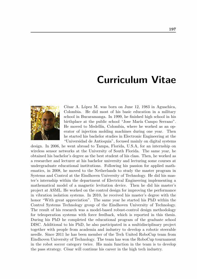
197
Curriculum Vitae
Cesar A. Lopez M. was born on June 12, 1983 in Aguachica,Colombia. He did most of his basic education in a militaryschool in Bucaramanga. In 1999, he finished high school in hisbirthplace at the public school “Jose Marıa Campo Serrano”.He moved to Medellın, Colombia, where he worked as an op-erator of injection molding machines during one year. Thenhe started his bachelor studies in Electronic Engineering at the“Universidad de Antioquia”, focused mainly on digital systems
design. In 2006, he went abroad to Tampa, Florida, U.S.A, for an internship onwireless sensor networks at the University of South Florida. The same year, heobtained his bachelor’s degree as the best student of his class. Then, he worked asa researcher and lecturer at his bachelor university and lecturing some courses atundergraduate educational institutions. Following his passion for applied math-ematics, in 2008, he moved to the Netherlands to study the master program inSystems and Control at the Eindhoven University of Technology. He did his mas-ter’s internship within the department of Electrical Engineering implementing amathematical model of a magnetic levitation device. Then he did his master’sproject at ASML. He worked on the control design for improving the performancein vibration isolation systems. In 2010, he received his master’s degree with thehonor “With great appreciation”. The same year he started his PhD within theControl Systems Technology group of the Eindhoven University of Technology.The result of his research was a model-based robust-control design methodologyfor teleoperation systems with force feedback, which is reported in this thesis.During his PhD he completed the educational program of the graduate schoolDISC. Additional to his PhD, he also participated in a multidisciplinary projecttogether with people from academia and industry to develop a robotic steerableneedle. Since 2011 he has been member of the Tech United RoboCup team fromEindhoven University of Technology. The team has won the RoboCup tournamentin the robot soccer category twice. His main function in the team is to developthe pass strategy. Cesar will continue his career in the high tech industry.

198