a meta-analysis of the price and income elasticities of
TRANSCRIPT

HAL Id: hal-02103880https://hal.archives-ouvertes.fr/hal-02103880
Submitted on 18 Apr 2019
HAL is a multi-disciplinary open accessarchive for the deposit and dissemination of sci-entific research documents, whether they are pub-lished or not. The documents may come fromteaching and research institutions in France orabroad, or from public or private research centers.
L’archive ouverte pluridisciplinaire HAL, estdestinée au dépôt et à la diffusion de documentsscientifiques de niveau recherche, publiés ou non,émanant des établissements d’enseignement et derecherche français ou étrangers, des laboratoirespublics ou privés.
Distributed under a Creative Commons Attribution - NonCommercial - NoDerivatives| 4.0International License
A meta-analysis of the price and income elasticities offood demandFabienne Femenia
To cite this version:Fabienne Femenia. A meta-analysis of the price and income elasticities of food demand. [Universityworks] Inconnu. 2019, 78 p. �hal-02103880�

A meta-analysis of the price and income elasticities of
food demand
Fabienne FEMENIA
Working Paper SMART – LERECO N°19-03
April 2019
UMR INRA-Agrocampus Ouest SMART - LERECO
(Laboratoires d’Etudes et de Recherches en Economie sur les Structures et Marchés Agricoles, Ressources et Territoires)

Working Paper SMART – LERECO N°19-03
Les Working Papers SMART-LERECO ont pour vocation de diffuser les recherches
conduites au sein des unités SMART et LERECO dans une forme préliminaire
permettant la discussion et avant publication définitive. Selon les cas, il s'agit de
travaux qui ont été acceptés ou ont déjà fait l'objet d'une présentation lors d'une
conférence scientifique nationale ou internationale, qui ont été soumis pour publication
dans une revue académique à comité de lecture, ou encore qui constituent un chapitre
d'ouvrage académique. Bien que non revus par les pairs, chaque working paper a fait
l'objet d'une relecture interne par un des scientifiques de SMART ou du LERECO et par
l'un des deux éditeurs de la série. Les Working Papers SMART-LERECO n'engagent
cependant que leurs auteurs.
The SMART-LERECO Working Papers are meant to promote discussion by
disseminating the research of the SMART and LERECO members in a preliminary form
and before their final publication. They may be papers which have been accepted or
already presented in a national or international scientific conference, articles which
have been submitted to a peer-reviewed academic journal, or chapters of an academic
book. While not peer-reviewed, each of them has been read over by one of the scientists
of SMART or LERECO and by one of the two editors of the series. However, the views
expressed in the SMART-LERECO Working Papers are solely those of their authors.
This work is licensed under a Creative Commons Attribution – Noncommercial – NoDerivatives 4.0 International

Working Paper SMART – LERECO N°19-03
1
A meta-analysis of the price and income elasticities of food demand
Fabienne FEMENIA
SMART-LERCO, AGROCAMPUS OUEST, INRA, 35000, Rennes, France
Acknowledgements:
This work has been partly financed by the International Food Policy Research Institute (IFPRI).
The author is grateful to David Laborde for his advises on the preliminary steps of this work,
to Laure Latruffe and two anonymous reviewers for their helpful comments on the paper and
to Christine Mesquida for her careful review of the references included in the meta-analysis.
Corresponding author
Fabienne Femenia
INRA, UMR SMART-LERECO
4 allée Adolphe Bobierre, CS 61103
35011 Rennes cedex, France
Email : [email protected]
Téléphone / Phone: +33(0)2 23 48 56 10
Les Working Papers SMART-LERECO n’engagent que leurs auteurs.
The views expressed in the SMART-LERECO Working Papers are solely those of their authors
Working Paper SMART – LERECO N°19-03
2
A meta-analysis of the price and income elasticities of food demand
Abstract
Food demand elasticities are crucial parameters in the calibration of simulation models used to
assess the impacts of political reforms or to analyse long-term projections, notably in
agricultural sectors. Numerous estimates of these parameters are now available in the economic
literature. The main objectives of this work are twofold: we seek first to identify general patterns
characterizing the demand elasticities of food products and second to identify the main sources
of heterogeneity between the elasticity estimates available in the literature. To achieve these
objectives, we conduct a broad literature review of food demand elasticity estimates and
perform a meta-regression analysis.
Our results reveal the important impacts of income levels on income and price elasticities both
at the country (gross domestic product-GDP) and household levels: the higher the income is,
the lower the level of elasticities. Food demand responses to changes in income and prices
appear to follow different patterns depending on the global regions involved apart from any
income level consideration. From a methodological viewpoint, the functional forms used to
represent food demand are found to significantly affect elasticity estimates. This result sheds
light on the importance of the specification of demand functions, and particularly of their
flexibility, in simulation models.
Keywords: elasticities, estimation, food demand, meta-analysis
JEL classification: Q11, Q18, D12, C13

Working Paper SMART – LERECO N°19-03
3
Une méta-analyse des élasticités prix et revenu de la demande de biens alimentaires
Résumé
Les élasticités prix et revenu de la demande de biens alimentaires sont des paramètres cruciaux
intervenant dans le calibrage des modèles de simulation qui sont utilisés pour évaluer l’impact
de réformes politiques ou faire des projections de long terme, notamment en ce qui concerne
dans les secteurs agricoles. De nombreuses valeurs estimées de ces paramètres sont aujourd’hui
disponibles dans la littérature économique. Nos principaux objectifs ici sont, d’une part, de
mettre en avant des éléments caractérisant de manière générale ces élasticités prix et revenu et,
d’autre part, d’identifier les principales sources de variabilité de leurs valeurs estimées dans la
littérature. Pour répondre à ce double objectif nous collectons dans la littérature un large
ensemble d’élasticités estimées de demande de biens alimentaires que nous analysons ensuite à
l’aide d’une méta-régression.
Nos résultats mettent en évidence un impact important du niveau de revenu, à la fois au niveau
pays (produit intérieur brut-PIB) et au niveau ménage, sur les élasticités prix et revenu : plus le
revenu est élevé, moins la demande de biens alimentaires est élastique. Il apparait également
que les réponses de la demande aux variations de revenu et de prix diffèrent entre régions du
monde indépendamment des différences de revenus pouvant exister entre ces régions. D’un
point de vue méthodologique, nous trouvons que le choix de la forme fonctionnelle utilisée pour
représenter la demande a un effet significatif sur les élasticités estimées. Ce résultat souligne
l’importance de la spécification des fonctions de demande, en particulier de leur flexibilité, dans
les modèles de simulation.
Mots-clés : élasticités, estimation, demande de biens alimentaires, méta-analyse
Classification JEL : Q11, Q18, D12, C13

Working Paper SMART – LERECO N°19-03
4
A meta-analysis of the price and income elasticities of food demand
1. Introduction
Simulation models, such as general or partial equilibrium models, are often used to analyse
long-term projections to assess the effects of political reforms or to shed light on a variety of
issues, notably in agricultural sectors. These models use a large number of behavioural
parameters, among which food demand elasticities play a crucial role (see, e.g., Rude and
Meilke (2004) and Carpentier et al. (2015)). Indeed, these parameters provide information on
how consumers react to income and price changes and are likely to have considerable impacts
on the simulation outcomes of projection and political reform scenarios for two main reasons.
First, the current global economic situation will undoubtedly evolve dramatically in the
forthcoming years even if economic policies remain unchanged. This is particularly true for
some developing countries in which incomes are expected to keep growing for several years.
Since the level of food consumption is a key element to be analysed for one who is interested
in economic projections, the impacts of income growth on household demand for food products,
which strongly depend on income elasticities, must be accounted for as accurately as possible
in simulation models. Second, even if agricultural policy reforms do not have strong impacts
on national income levels because agriculture generally represents a small proportion of Gross
Domestic Product (GDP), these reforms can have considerable impacts on agricultural prices.
Demand responses to price changes are thus of crucial importance when one wishes to simulate
the effects of agricultural policy reforms, and this depends on the value of food price elasticities.
Numerous price and income elasticity estimates are available in the economic literature and can
be used to calibrate large-scale simulation models. However, the studies from which these
estimates can be drawn use different types of data, rely on various assumptions regarding the
modelling of household food demand and use different econometric estimation methods. All
these sources of heterogeneity among studies may lead to significant variations in the empirical
estimates reported in the literature even if these estimates are supposed to measure the same
phenomenon, the responses of food demand to income or prices.
Our main objective in the present study is to investigate this issue by performing a meta-analysis
to identify and quantify the main sources of heterogeneity among the demand elasticity
estimates available in the literature.

Working Paper SMART – LERECO N°19-03
5
As emphasized by Nelson and Kennedy (2009), meta-analyses have been extensively used over
the past decades in several areas, including economics, to synthetize information provided by
empirical studies. Some meta-analyses of food demand elasticities have been conducted with
the stated objective of revealing “true” values of these parameters. Green et al. (2013) and
Cornelsen et al. (2016) notably conduct meta-analyses of own price and cross price elasticities
for various food products to provide estimates of these parameters by country income group.
Chen et al. (2016) also use a meta-analysis with the aim of providing estimates of price and
income elasticities of food demand in China. Our objective here is slightly different: we seek
to understand the heterogeneity of elasticity estimates across studies to help economists to select
empirical estimates of these key parameters for their simulation models. We aim at identifying
the key methodological aspects of primary studies that can have an impact on the values of
elasticity estimates beyond the factual elements that may affect elasticity values, such as the
type of food product or the country concerned. Our work also differs from Green et al. (2013)
and Cornelsen et al. (2016) by focusing not only on prices but also on income elasticities, which,
as explained above, can play a crucial role in long run projections and policy simulations.
Furthermore, compared to these two studies, additional variables characterizing elasticity
estimates are included in our analysis. We notably consider a more detailed categorization of
functional forms representing food demand, household income level, and information necessary
to assess publication bias, which is a pervasive issue among meta-analyses. Other meta-analyses
have been conducted to examine heterogeneity in these food demand elasticities estimates with
the aim of providing guidance on the study attributes to which attention should be paid. These
studies generally focus only on the type of product, such as alcohol (e.g., Fogarty, 2010; Nelson
2013a and 2013b; Sornpaisarn et al., 2013; Wagenaar et al., 2009) or meat (Gallet 2008 and
2010). Santeramo and Shabnam (2015), Melo et al. (2015), Ogundari and Abdulai (2013) and
Andreyeva et al. (2010) are exceptions since they consider various food products. However,
Santeramo and Shabnam (2015), Melo et al. (2015) and Ogundari and Abdulai (2013) do not
explicitly consider demand elasticities of food products but calorie- and/or nutrient-income
elasticities. The analysis conducted by Andreyeva et al. (2010) is essentially descriptive and
illustrates the potential heterogeneities that can exist between price elasticities estimates
without seeking to precisely identify the sources of such heterogeneity. We go deeper here by
relying on a meta-regression analysis (MRA) (Stanley and Jarell, 1989; Roberts, 2005). We
also pay particular attention to conforming to the meta-analysis guidelines provided by the
Meta-Analysis of Economics Research Network (MAER-NET) (Stanley et al., 2013), which

Working Paper SMART – LERECO N°19-03
6
defines key issues related to data searches and coding and modelling strategies, that must be
addressed in studies applying MRA to economics.
The next section is devoted to the description of the database of food demand elasticity
estimates that we build to fulfil our objectives. In the third section, a descriptive analysis is
presented to highlight several patterns characterizing own price and income elasticities in our
database and to identify potential sources of heterogeneity among elasticity estimates. These
sources are then statistically tested and quantified through an MRA in the fouth section, and
conclusions are drawn in the last section.
2. Data search and coding methods
In line with the MAER-NET protocol, we provide here a detailed description of how the
literature was searched and coded to build our database of price and income elasticity estimates.
The procedure used to collect the references included in the database is presented first. A second
part is devoted to the coding of information collected from primary studies. Finally, the
selection of the sample used in the meta-analysis is described in a third part.
2.1 Data collection
Diverse data sources are commonly used to calibrate demand functions in global economic
models (see, for instance, Valin et al. (2014) for a summary of data sources used in ten
computable general equilibrium and partial equilibrium models). Several models, such as
GCAM (Clarke et al., 2007), GLOBIOM (Havlik et al., 2011) and Mirage-BioF (Laborde and
Valin, 2012), use the price elasticities provided in two reports released by the United States
Department of Agriculture (USDA) (Seale et al. (2003a) and Muhammad et al. (2011)1) to
calibrate their demand function parameters. In these reports, price and income elasticities are
estimated for eight broad food categories (beverages and tobacco, bread and cereals, meat, fish,
dairy products, oils and fats, fruits and vegetables and other food products) and for a large
number of countries; own price and income elasticities are estimated for 114 countries in Seale
et al. (2003a) and for 144 countries in Muhammad et al. (2011). This broad level of country
coverage renders these elasticity data well-suited for calibrating large simulation models.
Economists might however wish to use other source of elasticities for different reasons when,
for instance, they consider food products at a higher disaggregation level or when they wish to
1 Muhammad et al. (2011) is an updated version of Seale et al. (2003a) considering more recent data and more
countries.

Working Paper SMART – LERECO N°19-03
7
compare results obtained with a calibration of demand parameters based on USDA estimates to
those obtained with a calibration based on other estimates given in the literature. The USDA
provides a literature review database (USDA, 2005), which contains this type of information
and is notably used to calibrate the IMPACT model (Robinson et al., 2015). This database
collects own price, cross price, expenditure and income demand elasticity estimates from papers
that have been published and/or presented in the United States (US) between 1979 and 2005.
This represents a total of 1,800 estimates of own price and income elasticities collected from
72 papers. While the database covers a large variety of products at various aggregation levels2,
few countries are included. The US is well-represented, with 1,166 elasticity estimates collected
from 44 papers, which is not surprising given the focus of the database on papers published or
presented in this country. The other elasticities are essentially for China with 528 estimates
collected from 22 papers, and only four other countries (Canada, Indonesia, Portugal and Saudi
Arabia) are represented, with a few estimates collected from up to three papers.
These two data sources, namely, the USDA’s estimates given in Seale et al. (2003a) and
Muhammad et al. (2011) and the USDA’s literature review database, were used to build the
database employed to conduct the meta-analysis presented here. More precisely, we started with
the structure of the USDA literature review database, which already includes useful information
on each elasticity estimate, such as the references of the papers from which the estimates have
been collected; the countries, products and time periods concerned; the types of data used to
conduct estimations; and the demand models estimated. The elasticities estimated by Seale et
al. (2003a) (1,824 estimates) and Muhammad et al. (2011) (2,304 estimates) were also included.
We then reviewed the primary studies to check the information included in the USDA database
and to ensure the consistency of the data. Of the 74 references present in these data, five PhD
dissertations were not available to us, thus restricting our ability to verify the data and to collect
new information, and we decided to exclude these references.
Then, to broaden the scope of the data, we searched for new references providing food demand
elasticity estimates in the economic literature with a focus on pre-2005 studies dealing with
countries other than the US and China and with a focus on post-2005 studies regardless of
country.
The search was performed with Google Scholar in March 2015 using the following
combinations of keywords: “price, elasticities, food, demand” and “income, elasticities, food,
2 Product aggregation levels vary from global food aggregate (e.g., Han et al., 1997) to very detailed levels (e.g.,
milk differentiated by fat level (Gould, 1996) or pasta sauces differentiated by brand (Seo and Capps, 1997)).

Working Paper SMART – LERECO N°19-03
8
demand”. We did not limit our search to published papers; working papers, reports, and papers
presented at conferences were also included. A total of 72 references were collected in this way.
All price and income elasticity estimates of food demand reported in these references were
collected. Among own price elasticities we distinguished uncompensated (Marshallian) price
elasticities from compensated (Hicksian) elasticities. This distinction is important since both
elasticities do not measure the same type of demand response to prices: uncompensated
elasticities measure the impact of a change in the price of one good by holding income and the
prices of other goods constant, and they thus incorporate both income (when the price of one
good increases, the income available to consume other goods decreases) and substitution effects
(when the price of one good increases, other goods become relatively less expensive);
compensated elasticities measure the impacts of a change in the price of one good holding
consumer utility constant, i.e., they assume that price changes are compensated by income
changes to maintain consumers’ utility levels and do not incorporate income effects. The two
types of price elasticities can thus not be considered equivalent or be studied simultaneously.
Given the small number of compensated own price elasticity estimates present in the USDA
literature review database and reported in the references that we collected (680 of 5,968 own
price elasticity estimates), we decided to focus on uncompensated price elasticities alone.
Our final database includes 3,334 own price elasticities and 3,311 income elasticity estimates
collected from 93 primary studies published between 1973 and 2014. Among these studies, a
significant number of papers, such as Seale et al. (2003a) and Muhammad et al. (2011), are
designed to provide estimates of food demand elasticities for subsequent use to understand the
structure of demand for food products or to simulate the evolution of such demand under
various scenarios. While Seale et al. (2003a) and Muhammad et al. (2011) include a large
number of countries, most of these papers focus on one particular country and provide estimates
for a complete set of food products or for one particular food sector, such as meat, dairy products
or fruits and vegetables. In other primary studies, food demand elasticities are estimated to
address specific empirical issues, such as the impacts of advertising, product differentiation,
health policies or structural changes, on the structure of food demand. Finally, several demand
elasticity estimates have been collected from primary studies that focused on methodological
aspects, such as the functional forms of demand models or the estimation procedures used to
estimate these models. In this case, elasticities are generally estimated for illustrative purposes
to assess the proposed approach.

Working Paper SMART – LERECO N°19-03
9
2.2 Information included and data coding
Based on the information collected during the review process, our database includes several
variables in addition to the values of elasticity estimates and the references of the primary
studies from which they have been collected3.
A first set of information included in our database relates to the primary data that have been
used to estimate the demand elasticities. Information relates to the type of data used (time series,
panel or cross section), to whether they have been collected at the micro (household) or macro
(country) level, to the decade in which they have been collected, which ranges from 1950 to
2010, and to the countries and products to which these data refer. To homogenize the
information on food products, product names as they appear in the primary studies are mapped
to the following eight product categories: beverages and tobacco, cereals, dairy products, fruits
and vegetables, oils and fats, meat and fish, other food products and non-food products. Given
that these categories are in some cases much broader than the product levels considered in
primary studies, a variable representing the aggregation level of the primary data is also
associated with each observation. The following four aggregation levels are considered: “global
food aggregate”; “product category aggregate”, which corresponds to the aforementioned
categories; “product level”, which refers to single products, for instance bananas and apples for
fruits, beef and poultry for meat, wheat and corn for cereals, etc.; “differentiated product level”,
which refers to products differentiated by specific characteristics, for instance, organic or
conventional for fruits and vegetables or cereals and types of cut for meat. Our mapping of
product names, product categories and aggregation levels is presented in Appendix 2. Country
names are converted into standard ISO-alpha-3 country codes (International Organization for
Standardization) and are mapped to 11 world regions according to the classification provided
in Appendix 3. Where applicable, we also report in our data information concerning the types
(urban, rural or any type) and levels of income of households from which the primary data have
been collected. While we also could have considered simple averages of elasticities for primary
studies reporting estimates for different household categories, as in Cornelsen et al. (2015), this
would have led to a loss of potentially important information. The levels of household income
are homogenized across studies by reporting these levels as a percentage of the highest income
considered in the study rather than as nominal income amounts.
3 Available human and financial resources did not allow for the data to be checked by an independent reviewer
as recommended under the MAER-NET protocol. An additional check was however performed by the author
herself to limit potential data coding errors.

Working Paper SMART – LERECO N°19-03
10
The second type of information included in the database relates to the precision of the elasticity
estimates. This information is indeed necessary for assessing an important issue of meta-
analysis, which is publication selection bias. Stanley (2005) identifies three sources of
publication bias as follows: (i) papers are more likely to be accepted for publication when they
conform to conventional views; (ii) when different models and/or estimation methods are
tested, authors are more likely to report results corresponding to conventional views; and (iii)
statistically significant results are treated more favourably. Hence, authors, reviewers and
journal editors may have a preference for statistically significant results in line with
conventional views, which results in studies finding small or insignificant estimates or estimates
with unexpected signs to remain unpublished. In our case, publication bias may lead food
demand elasticities to appear much larger in absolute terms than they actually are. It is thus
necessary as a first step in our meta-analysis to test for the presence of a publication selection
bias in our data. This can be accomplished by relying on a method proposed by Egger et al.
(1997), the PET test (precision effect test), which involves regressing effect size estimates
(demand elasticity estimates in our case) on an inverse indicator of their precision. This method
allows one to test both for the presence of a publication bias and for the existence of a “true”
effect size. Egger et al. (1997) suggest using the inverse standard errors of effect size estimates
as indicators of their precision and thus regressing effect sizes on standard errors of estimates.
When publication bias is detected, it must be accounted for in the subsequent meta-regression
analysis. Stanley and Doucouliagos (2014) recommend that the PEESE (precision effect
estimate with standard error) estimator be used in such cases, i.e., including the variances of
effect size estimates as explanatory variables in the meta-regression. This approach thus also
involves collecting information on the standard errors corresponding to each effect size
(demand elasticities in our case) estimates from the primary studies. Unfortunately, we face
here the same issue as that faced by other meta-analyses of demand elasticities: while studies
generally report standard errors of primary estimates (estimates of demand model parameters),
few report these elements for the elasticities that are computed from these estimates. In our
sample, less than 30% of estimated elasticities have associated standard error estimates and/or
Student’s t-test statistics, and we do not generally have sufficient information (complete
covariance matrix of estimates) to use delta methods to compute standard error elasticity
estimates. One solution involves only selecting studies with standard errors. This approach was
adopted by Ogundari and Abdulai (2013) in their study of calorie-income elasticities and by
Fogarty (2010) in his paper on alcohol demand elasticities. However, in our case, this would
have substantially reduced the sample size and thus limited the possibility of conducting an

Working Paper SMART – LERECO N°19-03
11
MRA. Some authors (Green et al., 2013; Cornelsen et al., 2015) do not treat publication bias
because of this lack of standard error data. To avoid this issue we use inverse sample sizes or
degrees of freedom (DF) instead of standard errors. Day (1999), among others, indeed
demonstrates the link between sample sizes and standard deviations of estimates, and Egger et
al. (1997) recommend the use of sample size or DF as a measure of precision in the absence of
standard error estimates. These two pieces of information are thus collected and added to our
database.
The last set of information included in our dataset relates to methodological aspects of
elasticities estimations. We collected here all relevant information that could potentially help
to explain the heterogeneity among elasticity estimates. This information essentially concerns
the following econometric and modelling strategies adopted in primary studies: the functional
form of the demand system from which elasticities are estimated; reliance on a multi-stage
budgeting structure; the way in which zero values are treated in the estimation process; the use
of unit values or quality adjusted prices; the inclusion of control variables related to household
characteristics, product characteristics or time periods; and the econometric method used to
estimate the demand model.
2.3 Sample selection
This subsection presents the selection procedure applied to the data sample used for the meta-
analysis.
A first round of data selection was conducted based on the aggregation level of food products
considered in the data used in the primary studies. Two of the four product aggregation levels
identified in our dataset were excluded from the analysis as follows: the “global food aggregate”
level and the “differentiated product” level, which includes very specific products that are of
little relevance for large simulation models and for which elasticity estimates tend to be
extremely high in absolute terms. This selection approach led to us exclude 42 primary studies
and 1,959 elasticity estimates.
Then, we excluded primary studies that did not provide the number of observations used to
estimate the elasticities since, as previously mentioned, this information is used as a proxy for
the precision of elasticity estimates in the MRA. This selection approach led us to exclude 5
primary studies and 372 elasticity estimates.

Working Paper SMART – LERECO N°19-03
12
We do not consider in our analysis the “non-food” and “beverage and tobacco” product
categories, which correspond to 809 elasticity estimates. The “non-food” category indeed falls
outside of the scope of our study and the demand for “beverage and tobacco” exhibits very
specific patterns, which explains why a large number of meta-analyses have already been
conducted on these products specifically.
Finally, as in Cornelsen et al. (2015), we consider as outliers price and income elasticities
ranging outside of three standard deviations of their respective averages and exclude such
outliers from our sample. This represents 63 observations for price elasticities and 41
observations for income elasticities.
The sample of elasticity estimates considered the paper thus includes 6,645 observations
collected from 93 primary studies, among which 3,334 are price elasticities and 3,311 are
income elasticities.
2. Descriptive analysis of the data
After discussing how price and income demand elasticities may differ across product categories
and world regions, this section highlights other potential sources of heterogeneity among
estimates related to the methodological approaches adopted in the primary studies.
2.1 Heterogeneity of elasticity estimates across food products
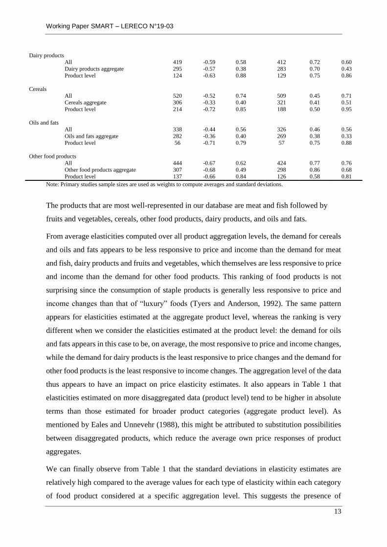
Table 1 reports, by product category and aggregation level sub-categories, the number of
observations, weighted averages and standard deviations of price and income elasticities. More
weight is given to more precise estimates in the computation of averages and standard
deviations.
Table 1: Elasticities - summary statistics by food product categories
Own Price elasticities Income elasticities
Nb Obs. Weighted
Average
Weighted
S.D.
Nb Obs. Weighted
Average
Weighted
S.D.
Fruits and vegetables
All 668 -0.61 0.69 694 0.61 0.68
Fruits and vegetables aggregate 327 -0.50 0.47 308 0.53 0.43
Product level 341 -0.71 0.79 386 0.67 0.81
Meat and fish
All 945 -0.57 0.53 946 0.73 0.66
Meat and fish aggregate 554 -0.50 1.09 579 0.67 0.43
Product level 391 -0.66 3.85 367 0.83 0.88
Working Paper SMART – LERECO N°19-03
13
Dairy products
All 419 -0.59 0.58 412 0.72 0.60
Dairy products aggregate 295 -0.57 0.38 283 0.70 0.43
Product level 124 -0.63 0.88 129 0.75 0.86
Cereals
All 520 -0.52 0.74 509 0.45 0.71
Cereals aggregate 306 -0.33 0.40 321 0.41 0.51
Product level 214 -0.72 0.85 188 0.50 0.95
Oils and fats
All 338 -0.44 0.56 326 0.46 0.56
Oils and fats aggregate 282 -0.36 0.40 269 0.38 0.33
Product level 56 -0.71 0.79 57 0.75 0.88
Other food products
All 444 -0.67 0.62 424 0.77 0.76
Other food products aggregate 307 -0.68 0.49 298 0.86 0.68
Product level 137 -0.66 0.84 126 0.58 0.81
Note: Primary studies sample sizes are used as weights to compute averages and standard deviations.
The products that are most well-represented in our database are meat and fish followed by
fruits and vegetables, cereals, other food products, dairy products, and oils and fats.
From average elasticities computed over all product aggregation levels, the demand for cereals
and oils and fats appears to be less responsive to price and income than the demand for meat
and fish, dairy products and fruits and vegetables, which themselves are less responsive to price
and income than the demand for other food products. This ranking of food products is not
surprising since the consumption of staple products is generally less responsive to price and
income changes than that of “luxury” foods (Tyers and Anderson, 1992). The same pattern
appears for elasticities estimated at the aggregate product level, whereas the ranking is very
different when we consider the elasticities estimated at the product level: the demand for oils
and fats appears in this case to be, on average, the most responsive to price and income changes,
while the demand for dairy products is the least responsive to price changes and the demand for
other food products is the least responsive to income changes. The aggregation level of the data
thus appears to have an impact on price elasticity estimates. It also appears in Table 1 that
elasticities estimated on more disaggregated data (product level) tend to be higher in absolute
terms than those estimated for broader product categories (aggregate product level). As
mentioned by Eales and Unnevehr (1988), this might be attributed to substitution possibilities
between disaggregated products, which reduce the average own price responses of product
aggregates.
We can finally observe from Table 1 that the standard deviations in elasticity estimates are
relatively high compared to the average values for each type of elasticity within each category
of food product considered at a specific aggregation level. This suggests the presence of

Working Paper SMART – LERECO N°19-03
14
additional sources of heterogeneity in elasticities, with one being location, as discussed in the
following subsection.
2.2 Heterogeneity of elasticity estimates across regions
Consumption patterns can differ between countries for several reasons, including differences in
tastes (see, e.g., Selvanathan and Selvanathan, 1993), implying variations in demand elasticities
across countries. Table 2 reports the weighted averages and standard deviations of demand
elasticity estimates for the 11 world regions and six product categories that we consider.
We first note that again, standard deviations of elasticity estimates are relatively high compared
to their average values and for the countries that are most well-represented in the database in
particular, namely, North American, Asian and European Union (EU) countries.

Working Paper SMART – LERECO N°19-03
15
Table 2. Elasticities - summary statistics by world regions
Own price elasticities Income elasticities
Cerea
ls Dairy
Fruit
and
veg.
Meat
Oils
and
Fat
Other
food
Cerea
ls Dairy
Fruit
and
veg.
Meat
Oils
and
Fat
Other
food
North America
Weighted
average -0.68 -0.41 -0.75 -0.62 -0.32 -0.41
0.68 0.52 0.69 0.71 0.48 0.62
Weighted S.D. 0.61 0.66 0.74 0.49 0.47 0.58 0.89 0.67 0.91 0.78 0.72 0.83
Nb Obs. 64 33 98 156 17 44 47 30 66 115 17 29
Latin America
Weighted
average -0.36 -0.58 -0.50 -0.54 -0.37 -0.61
0.42 0.84 0.62 0.74 0.49 0.72
Weighted S.D. 0.41 0.50 0.43 0.36 0.46 0.30 0.46 0.60 0.56 0.53 0.51 0.59
Nb Obs. 34 37 37 71 34 34 52 53 91 83 40 52
East Asia
Weighted
average -0.63 -0.69 -0.67 -0.66 -0.64 -0.64
0.55 0.71 0.73 0.82 0.66 0.77
Weighted S.D. 0.82 0.84 0.73 0.84 0.78 0.90 0.86 0.79 0.78 0.76 1.09 0.76
Nb Obs. 81 48 95 137 33 31 69 56 142 163 30 46
Asia Other
Weighted
average -0.59 -0.53 -0.64 -0.53 -0.59 -0.71
0.36 0.78 0.56 0.71 0.52 0.74
Weighted S.D. 0.86 0.55 0.79 0.54 0.52 0.66 0.82 0.68 0.79 0.77 0.51 0.86
Nb Obs. 122 70 157 121 47 92 116 57 134 126 35 74
European Union
Weighted
average -0.19 -0.55 -0.49 -0.49 -0.17 -0.53
0.25 0.64 0.45 0.69 0.22 0.61
Weighted S.D. 0.41 0.65 0.64 0.51 0.21 0.38 0.46 0.63 0.56 0.79 0.27 0.52
Nb Obs. 63 76 108 165 54 75 65 69 91 168 54 74
European Other
Weighted
average -0.42 -0.62 -0.70 -0.54 -0.42 -0.77
0.24 0.32 0.39 0.41 0.21 0.42
Weighted S.D. 0.66 0.56 0.86 0.62 0.60 0.75 0.33 0.19 0.23 0.18 0.22 0.43
Nb Obs. 12 12 12 18 12 12 12 12 12 18 12 12

Working Paper SMART – LERECO N°19-03
16
Own price elasticities Income elasticities
Cerea
ls Dairy
Fruit
and
veg.
Meat
Oils
and
Fat
Other
food
Cerea
ls Dairy
Fruit
and
veg.
Meat
Oils
and
Fat
Other
food
Former Soviet
Union
Weighted
average -0.32 -0.59 -0.43 -0.55 -0.34 -0.68
0.42 0.77 0.56 0.71 0.44 0.89
Weighted S.D. 0.16 0.14 0.12 0.20 0.15 0.19 0.19 0.13 0.12 0.21 0.17 0.31
Nb Obs. 32 32 32 64 32 32 32 32 32 64 32 32
Middle East
Weighted
average -0.58 -0.66 -0.62 -0.59 -0.56 -0.77
0.35 0.68 0.50 0.67 0.38 0.74
Weighted S.D. 0.87 0.37 0.48 0.36 0.84 0.35 0.31 0.21 0.16 0.42 0.28 0.49
Nb Obs. 34 34 43 62 34 50 26 26 27 55 26 28
North Africa
Weighted
average -0.33 -0.57 -0.42 -0.52 -0.34 -0.70
0.43 0.75 0.55 0.69 0.45 0.93
Weighted S.D. 0.09 0.06 0.06 0.12 0.08 0.31 0.11 0.10 0.09 0.13 0.10 0.48
Nb Obs. 5 5 5 10 5 5 5 5 5 10 5 5
Sub Saharan
Africa
Weighted
average -0.50 -0.68 -0.56 -0.60 -0.44 -0.92
0.60 0.84 0.66 0.80 0.61 1.06
Weighted S.D. 0.55 0.39 0.52 0.29 0.22 0.64 0.59 0.23 0.43 0.31 0.27 0.93
Nb Obs. 67 66 75 129 64 63 79 66 88 132 69 66
Oceania
Weighted
average -0.16 -0.42 -0.30 -0.39 -0.19 -0.48
0.21 0.55 0.39 0.51 0.25 0.63
Weighted S.D. 0.22 0.21 0.17 0.20 0.20 0.33 0.29 0.29 0.22 0.26 0.26 0.47
Nb Obs. 6 6 6 12 6 6 6 6 6 12 6 6
Note: Primary studies sample sizes are used as weights to compute averages and standard deviations.

Working Paper SMART – LERECO N°19-03
17
Table 2 shows greater variation in demand elasticities across regions for a given product than
across products for a given region. Geographical aspects thus appear to have an important
impact on demand elasticities. No clear regional pattern arises from the mean elasticities
reported in Table 2, which is in fact not surprising given the variability in the data. One can
however expect countries’ income levels to have substantial impacts on demand elasticities.
Indeed, income increases associated with economic development are expected to have
considerable impacts on global food demand, and it is now widely recognized in the economic
literature that an increase in household income not only leads to an increase in global
consumption but also to a modification of consumption structures. Indeed, an income increase
is expected to lead first to a decrease in the share of expenditures devoted to food consumption
and second to a decrease in raw products among food expenditures. These two properties, which
are formalized respectively by Engel’s and Bennet’s laws, imply that food demand becomes
less responsive to income and price changes as income rises (Timmer et al., 1983). The demand
elasticities of food products, and particularly those of raw products, are thus expected to
decrease (in absolute terms) with income. While not obvious in Table 2, these demand patterns
clearly appear on Figures 1 and 2, in which we report the average estimated income and own
price elasticities for each country with respect to their GDP per capita for 2005. These figures
show that, although income and price elasticities are systematically higher for some products
(e.g., meat) than for others (e.g., oils and fats), both tend to decrease with GDP per capita in
absolute terms.

Working Paper SMART – LERECO N°19-03
18
Figure 1: Evolution of income elasticities with GDP per capita
Figure 2. Evolution of price elasticities with GDP per capita
-0,5
0
0,5
1
1,5
2
0 10000 20000 30000 40000 50000 60000 70000 80000 90000
Ave
rage
inco
me
elas
tici
ties
per
co
un
try
GDP per capita (US dollars)
cereals dairy fruits and veg.
meat oils and fat other food
tendency curve - cereals tendency curve - dairy tendency curve - fruits and veg.
tendency curve - meat tendency curve - oils and fat tendency curve - other food
-1,8
-1,6
-1,4
-1,2
-1
-0,8
-0,6
-0,4
-0,2
0
0,2
0 10000 20000 30000 40000 50000 60000 70000 80000 90000
Ave
rage
pri
ce e
last
icit
y p
er c
ou
ntr
y
GDP per capita (US dollars)
cereals dairy fruits and veg.
meat oils and fat other food
tendency curve- celeals tendency curve - dairy tendency curve - fruits and veg.
tendency curve- meat tendency curve - oils and fat tendency curve - other food
Working Paper SMART – LERECO N°19-03
19
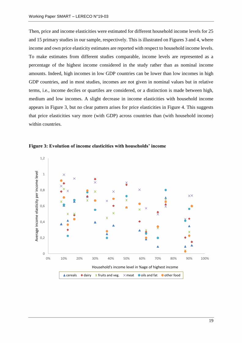
Then, price and income elasticities were estimated for different household income levels for 25
and 15 primary studies in our sample, respectively. This is illustrated on Figures 3 and 4, where
income and own price elasticity estimates are reported with respect to household income levels.
To make estimates from different studies comparable, income levels are represented as a
percentage of the highest income considered in the study rather than as nominal income
amounts. Indeed, high incomes in low GDP countries can be lower than low incomes in high
GDP countries, and in most studies, incomes are not given in nominal values but in relative
terms, i.e., income deciles or quartiles are considered, or a distinction is made between high,
medium and low incomes. A slight decrease in income elasticities with household income
appears in Figure 3, but no clear pattern arises for price elasticities in Figure 4. This suggests
that price elasticities vary more (with GDP) across countries than (with household income)
within countries.
Figure 3: Evolution of income elasticities with households’ income
0
0,2
0,4
0,6
0,8
1
1,2
0% 10% 20% 30% 40% 50% 60% 70% 80% 90% 100%
Ave
rage
inco
me
elas
tici
ty p
er in
com
e le
vel
Household's income level in %age of highest income
cereals dairy fruits and veg. meat oils and fat other food

Working Paper SMART – LERECO N°19-03
20
Figure 4: Evolution of price elasticities with households’ income
3. Methodological sources of heterogeneity in elasticity estimates
Elasticity estimates collected from different primary studies display strong levels of
heterogeneity, part of which can be attributed to the data based on which they have been
estimated in terms of product and country or household income. However, as illustrated by the
standard deviations reported in Tables 1 and 2 and by the dispersion of data in Figures 1 to 4, a
significant proportion of the heterogeneity across elasticity estimates remains unexplained by
these elements. We discuss here some characteristics that are essentially related to
methodological issues that differ across the studies and that might be at the root of this
additional heterogeneity across study estimates. These characteristics notably concern the
flexibility of the functional forms used to represent household demand, the treatment of zero
values in econometric estimations of demand systems, and the definition of the “price variable”
used to estimate demand systems.
Diverse functional forms representing consumer demand are used in primary studies to estimate
price and income elasticities. Among them is the Rotterdam model introduced by Barten (1964)
and Theil (1965). The popularity of this model has already been noted by Clements and Gao
-1,4
-1,2
-1
-0,8
-0,6
-0,4
-0,2
0
0% 10% 20% 30% 40% 50% 60% 70% 80% 90% 100%
Ave
rage
pri
ce e
last
icit
y p
er in
com
e le
vel
Household's income level in %age of highest income
cereals dairy fruits and veg. meat oils and fat other food

Working Paper SMART – LERECO N°19-03
21
(2015), who review the methodological developments that have occurred over the past fifty
years in applied demand analysis and demonstrate the importance of the Rotterdam model in
this respect. This model is derived in an unconventional way in the sense that it does not require
the specification of a specific type of cost or utility function. Other popular demand systems,
such as the Linear Expenditure System (LES) (Stone, 1954), the Translog system (Christensen
et al., 1975), and the Almost Ideal Demand System (AIDS) (Deaton and Muellbauer, 1980),
are indeed more traditionally derived from the optimization of specific (indirect) utility or
expenditure functions. Clements and Gao (2015), however, show that these systems can
actually be reformulated as differential systems relatively similar to the Rotterdam model and
can thus be considered to belong to the same class of differential demand systems as that of
Rotterdam4.
Almost 7% of the primary studies included in our sample rely on the Rotterdam model. The
LES and Translog systems are adopted in respectively 3% and 5% of the primary studies
included in our sample. The AIDS and its linearized version, the LA-AIDS5, are the most well-
represented demand systems, with 20% and 36% of primary studies relying on them,
respectively. A generalization of the AIDS, the quadratic AIDS (QUAIDS) developed by Banks
et al. (1997), is also used in 13% of the studies. In this model, budget shares are assumed to be
quadratic functions of the log of income rather than linear functions, as they are in AIDS. This
specification offers more flexibility in the representation of demand since income elasticities
are allowed to vary with income levels. It should finally be noted that, contrary to ad hoc single
equations sometimes used to estimate demand elasticities (in 5% of primary studies included in
our sample), all the aforementioned demand systems are theoretically consistent since they have
been built to satisfy the homogeneity, symmetry and adding-up constraints imposed by the
economic theory of demand. The only theoretical property that might not necessarily be
satisfied is the concavity in price of the expenditure function, which translates into the negative
semi-definiteness of the Slutsky matrix. These restrictions can, however, be imposed in
econometric estimations (see, e.g., Moschini (1998 and 1999) and Ryan and Wales (1998)).
4 The CBS model (Keller and van Driel, 1985) and the NBR model (Neves, 1994) are two other popular models
related to the Rotterdam model. Our sample, however, includes only one primary study relying on a CBS model
and none that rely on an NBR model.
5 The LA-AIDS is an approximation of the AIDS in which the linear Stone price index is used in place of the
“true” AIDS price index to ease econometric estimations.

Working Paper SMART – LERECO N°19-03
22
Finally, should be noted that 11% of the primary studies use other specific models to obtain
demand elasticities6.
Furthermore, 18% of the studies rely on multi-stage budgeting frameworks that first allocate
consumer food expenditures to broad product categories or groups based on group-specific
price indices and then to smaller aggregates within each category, with within-groups budget
allocation performed independently. By reducing the number of parameters to be estimated this
nesting structure allows one to consider demand systems with more disaggregated products. It
relies on the assumption of weak separability between goods, i.e., a change in price for one
product in one category is assumed to affect the demand for all products in other categories in
the same way, and on the assumption of low variability in group-specific price indices with
expenditures (Edgerton, 1997). As emphasized by Edgerton (1997) and Carpentier and
Guyomard (2001), multi-stage budgeting has important implications in terms of estimated
income and price elasticities since specific formulas must be used to recover total or
unconditional elasticities from estimates made for group or conditional elasticities. Given that
our analysis focuses on the total impacts of income or price changes on food product demand,
we consider only the unconditional elasticities estimates reported in primary studies. The
specific structure of multi-stage budgeting frameworks and their underlying assumptions might
however have some effects on these estimated unconditional elasticities.
Another methodological difference observed across the studies concerns the treatment of corner
solutions. Datasets used to estimate demand models frequently contain a significant number of
zeros since not all products are consumed by all consumers. This is all the more true when
products are considered at disaggregated levels and in micro-econometric studies relying
individual or household data. These zero values generate corner solutions, which can be a
problem for econometric estimations of demand systems. This issue can be avoided by
removing zeros in datasets by excluding the corresponding observations or by considering
sufficiently aggregated data. This is the case for 35% of the studies included in our database.
Other studies, however, tackle the issue and account for censored demand in their econometric
6 Among these models are the Florida model used by Seale et al. (2003a) and Muhammad et al. (2011), the LinQuad
model used by Fang and Beghin (2002) and Fabiosa and Jensen (2003), the CBS model used by Hahn (2001) and
the AIDADS model used by Yu et al. (2004). Since these models are rarely used in our data, they have been
grouped into a category termed “other” in our empirical application. Regarding the number of observations, this
category is dominated by the Florida model since Seale et al. (2003a) and Muhammad et al. (2011) report 1,824
and 2,304 elasticity estimates, respectively.

Working Paper SMART – LERECO N°19-03
23
estimations. Different means of addressing corner solutions have been proposed in the
economic literature. In particular, Wales and Woodland (1983) and Lee and Pitt (1986), relying
respectively on endogenous regime switching and virtual prices approaches, offer theoretically
consistent frameworks to account for censored demands. However, these approaches are
difficult to use in empirical applications, particularly when large datasets are considered.
Empirical procedures have thus been developed to deal with censored demand, among which
is the seminal work of Heien and Wessels (1990). A few years later, the approach proposed by
Shonkwiler and Yen (1999) was published and is now commonly used in the literature. In the
spirit of Heckman’s two-step estimator (1979), the estimator proposed by Shonkwiler and Yen
(1999) involves first estimating a probit model and then conducting a regression that accounts
for censoring through the introduction of correction terms that derive from the probit estimates.
Although easy to implement, this estimator might lack efficiency, as do other two-step
estimators (Wales and Woodland, 1983), and may lead to biased results in cases of
distributional misspecification (Schafgans, 2004). Alternative approaches based, for instance,
on simulated maximum likelihood approaches (Yen et al., 2003) and semiparametric
econometrics (Sam and Zheng, 2010) have recently been proposed as means to overcome these
issues.
The last methodological issue that deserves discussion relates to prices used to estimate demand
systems. The datasets used to estimate demand systems do not generally explicitly contain price
information mainly because prices paid by households are usually not directly observable and
because goods are aggregated. A standard procedure involves using unit values (expenditures
divided by quantities) as proxies for prices, but, as explained by Huang and Lin (2000), this is
not fully satisfactory since other information related to food quality is given in unit values. One
solution involves following the approach proposed by Deaton (1988), which allows one to
extract quality effects from unit values. In spite of the potential biases induced by the use of
unit values to estimate price elasticities, 95% of the studies still use them as proxies for product
prices while 5% only rely on quality-adjusted prices as proposed by Deaton (1988).
To account for these methodological issues, we introduced into the database the following four
additional variables: a “model” variable with eight modalities corresponding to the various
functional forms used to model demand and three dummy variables indicating whether multi-
stage budgeting, the treatment of corner solutions and quality adjusted prices, have been used
in the primary studies.

Working Paper SMART – LERECO N°19-03
24
We also added three dummy variables to account for the fact that econometric estimations of
demand systems often include several variables in addition to prices and incomes. Control
variables are indeed introduced in the primary studies’ econometric estimations for three main
reasons. The dummy variables “hetero_indiv”, “hetero_time” and “hetero_product” indicate
whether demographic characteristics have been used to control for heterogeneity across
households, whether time dummies and trends have been used to account for the evolution of
consumer demand and preferences over time and whether product brand or advertisement
characteristics have been used to control for product heterogeneity, respectively.
Finally, Cornelsen et al. (2016) find estimation methods to have an impact on the estimated
values of price elasticities. To control for this potential effect, we included in our database a
variable reporting the econometric method used to conduct the estimations in the primary
studies. We adopted the same classification as that used in Cornelsen (2016) to introduce a
variable taking the following four modalities: seemingly unrelated regression (SUR), ordinary
least squares regression, maximum likelihood estimation and other methods. We must,
however, acknowledge that the distinction between the different methods is not always
straightforward since, for instance, the iterative SUR estimation method often used to impose
regularity condition on demand systems is asymptotically equivalent to a maximum likelihood
approach. Here, we decided to classify iterative SUR methods under the “SUR” category.
4. Meta regression analysis
Having described the potential sources of heterogeneity across price and income elasticity
estimates found in the literature, we perform an MRA of our data to identify and quantify these
sources of heterogeneity in a statistically consistent manner.
4.1 Methodology
Two sets of MRA, one for price elasticities and one for income elasticities, are performed.
The MAER-NET protocol (Stanley et al., 2013) identifies publication selection bias,
heteroscedasticity and within-studies dependence as key issues to be approached through MRA.
As explained in section 2.2, we use the PET test proposed by Egger et al. (1997) to test for
publication selection bias. When publication bias is detected, it is accounted for by introducing

Working Paper SMART – LERECO N°19-03
25
a measure of the precision of estimates as an explanatory variable in the MRAs in line with the
method proposed by Stanley and Doucouliagos (2014).
Heteroscedasticity issues may arise during MRA because the variances of effect size estimates
vary from one primary study to another for several reasons, including differences in sample
size, sample observations or estimation procedures (Nelson and Kennedy, 2009). One
straightforward means to account for this heteroscedasticity involves using a weighted least
square (WLS) approach and to give more weight to the more precise estimate, i.e., to elasticity
estimates with the lowest level of estimated variance. However, as noted above, very few
studies included in our sample report variance in price and income elasticity estimates. We thus
use primary studies’ sample sizes as proxies to these variances, which is a common procedure
used in MRA studies and notably in environmental economics (Nelson and Kennedy, 2009).
Other issues can arise in the presence of correlations of effect size estimates within and between
primary studies. Indeed, our data contain several elasticity estimates collected from each
primary study. However, if most characteristics distinguishing estimates from the same study
(product category, household income level, demand functional form, econometric estimation
method, etc.) are introduced as explanatory variables and thus are controlled for in our MRAs,
some unobservable characteristics may give rise to correlated error terms across elasticities
collected from the same primary study. In the same way, primary studies conducted by the same
author may share unobservable characteristics and may lead to between studies correlations. To
overcome this issue, we follow the same approach that was used by Disdier and Head (2008)
and Cipollina and Salvatici (2010) and introduce random study/author effects into the MRA
models. This results in the generation of mixed-effect models, which can be defined as
multilevel regression models (Bateman and Jones, 2003) and are formally expressed as:
𝜃𝑖𝑗 = 𝛼0 + ∑ 𝛼𝑘𝑋𝑘
𝐾
𝑘=1
+ 𝑢𝑖 + 𝜀𝑖𝑗 (1)
where 𝜃𝑖𝑗 is the dependent variable and denotes the j-th (price or income) elasticity estimate
collected from the i-th primary study (or i-th author), 𝛼0 is a fixed intercept and 𝛼𝑘 (𝑘 ∈
{1, … , 𝐾}) is the fixed effect coefficient associated with 𝐾 explanatory variable 𝑋𝑘 (𝑘 ∈
{1, … , 𝐾}). 𝜀𝑖𝑗 is normally distributed with constant variance and can be interpreted as a
sampling error term. 𝑢𝑖 is a random study (or author) effect that is normally distributed with
constant variance independent of 𝜀𝑖𝑗 and is assumed to be uncorrelated with the explanatory
variables. Adding this random effect to the MRA model allows one to account for correlations
Working Paper SMART – LERECO N°19-03
26
between elasticity estimates of primary studies/authors (Nelson and Kennedy, 2009)7. In this
way, we also depart from the assumption that, conditional on the observed characteristics
represented by the explanatory variables, all primary studies estimate exactly the same level of
elasticity. Here, elasticity estimates are assumed to be comparable but not exactly the same
across studies/authors (Nelson, 2013a), and the primary studies included in our data are
assumed to form a random sample of a universe of potential studies (Borenstein et al., 2010).
The soundness of this assumption was notably underscored by Higgins and Thompson (2002),
who clearly argue for the introduction of random effects into MRA models. Nelson and
Kennedy (2009) assert that mixed models may lead to bias fixed effect coefficient estimates if
random effects are correlated with one or more explanatory variables. We assume that this is
not the case here, which appears to be a reasonable assumption given that most of our
explanatory variables are dummies representing characteristics that are not associated with only
one author or study. Additionally, Nelson and Kennedy (2009, p. 358) conclude that “the
advantages of random-effects estimation are so strong that this estimation procedure should be
employed unless a very strong case can be made for its appropriateness”.
4.2 Test for publication bias
PET tests are performed to check for the presence of publication bias in our data. These tests
involve regressing elasticity estimates on an inverse indicator of their precision. The following
two sets of regressions are performed: one for price and one for income elasticities. Given the
lack of standard errors of effect size estimates included in our data, we consider two alternative
indicators of their precision including the inverse square root of the primary sample size and
the inverse square root of DF. Stanley and Doucouliagos (2014) also recommend the use of
WLS regressions with inverse standard errors as weights to deal with heteroscedasticity issues.
We follow their proposed approach and use as weights the square roots of sample sizes or DF
depending on which indicator we use for the regression.
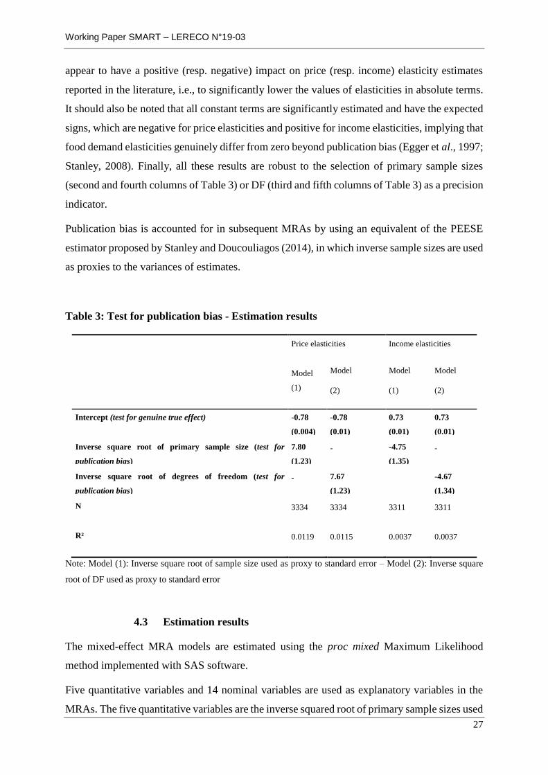
Estimation results are reported in Table 3. We find that the coefficients associated with the
inverse precision criteria are significantly estimated in all cases, implying that publication
selection bias exists in our data both for price (second and third columns of Table 3) and for
income (fourth and fifth columns of Table 3) elasticities. Inverse precision indicators actually
7 The variance-covariance matrix of the composite error term of the model (𝑢𝑖 + 𝜀𝑖𝑗) is block-diagonal allowing
for within-study (or within) author correlations.
Working Paper SMART – LERECO N°19-03
27
appear to have a positive (resp. negative) impact on price (resp. income) elasticity estimates
reported in the literature, i.e., to significantly lower the values of elasticities in absolute terms.
It should also be noted that all constant terms are significantly estimated and have the expected
signs, which are negative for price elasticities and positive for income elasticities, implying that
food demand elasticities genuinely differ from zero beyond publication bias (Egger et al., 1997;
Stanley, 2008). Finally, all these results are robust to the selection of primary sample sizes
(second and fourth columns of Table 3) or DF (third and fifth columns of Table 3) as a precision
indicator.
Publication bias is accounted for in subsequent MRAs by using an equivalent of the PEESE
estimator proposed by Stanley and Doucouliagos (2014), in which inverse sample sizes are used
as proxies to the variances of estimates.
Table 3: Test for publication bias - Estimation results
Price elasticities Income elasticities
Model
(1)
Model
(2)
Model
(1)
Model
(2)
Intercept (test for genuine true effect) -0.78
(0.004)
-0.78
(0.01)
0.73
(0.01)
0.73
(0.01)
Inverse square root of primary sample size (test for
publication bias)
7.80
(1.23)
- -4.75
(1.35)
-
Inverse square root of degrees of freedom (test for
publication bias)
- 7.67
(1.23)
-4.67
(1.34)
N 3334 3334 3311 3311
R² 0.0119 0.0115 0.0037 0.0037
Note: Model (1): Inverse square root of sample size used as proxy to standard error – Model (2): Inverse square
root of DF used as proxy to standard error
4.3 Estimation results
The mixed-effect MRA models are estimated using the proc mixed Maximum Likelihood
method implemented with SAS software.
Five quantitative variables and 14 nominal variables are used as explanatory variables in the
MRAs. The five quantitative variables are the inverse squared root of primary sample sizes used

Working Paper SMART – LERECO N°19-03
28
to correct for publication bias, the country’s GDP, the household income level and the two time
trends corresponding to the publication date of the primary studies and to the decade of the data
used to estimate elasticities. The 14 nominal explanatory variables are listed in Table 4. Most
of these variables have already been discussed in section 3 except for the “Urban vs rural
households” variable, which indicates whether the elasticity has been estimated for an urban
population, a rural population or the general population without distinctions made between rural
and urban areas. For each nominal variable, the modality serving as a baseline reference is
highlighted in Table 4.
Table 4: Descriptive statistics of the variables introduced in the meta-regression-
Summary statistics
Own price elasticities Income elasticities
Average
elasticity Nb Obs
Average
elasticity Nb Obs
Type of data
Panel -0.72 129 0.66 80
Cross section -0.58 2804 0.63 2900
Time series -0.66 401 0.69 331
Data level
Individual -0.70 1154 0.70 1153
Country -0.47 2180 0.59 2158
Product
Dairy -0.59 419 0.72 412
Fruits and vegetables -0.61 668 0.61 694
Meat and fish -0.57 945 0.73 946
Oils and fats -0.44 338 0.46 326
Other food products -0.67 444 0.77 424
Cereals -0.52 520 0.45 509
Product aggregation level
Product level -0.68 1263 0.69 1253
Aggregate level -0.49 2071 0.60 2058

Working Paper SMART – LERECO N°19-03
29
Own price elasticities Income elasticities
Average
elasticity Nb Obs
Average
elasticity Nb Obs
Region
Latin America -0.50 247 0.65 371
East Asia -0.66 425 0.73 506
Asia Other -0.60 609 0.59 542
European Union -0.43 541 0.52 521
Europe Other -0.57 78 0.34 78
Former Soviet Union -0.49 224 0.64 224
Middle East -0.64 257 0.57 188
North Africa -0.49 35 0.63 35
Sub-Saharan Africa -0.61 464 0.75 500
Oceania -0.33 42 0.43 42
North America -0.61 412 0.65 304
Urban vs rural households
Urban -0.62 360 0.64 346
Rural -0.62 321 0.76 385
No distinction -0.55 2653 0.61 2580
Demand model
LA-AIDS -0.71 503 0.82 388
AIDS -0.84 575 0.79 229
QUAIDS -0.78 449 0.64 319
Rotterdam -0.44 33 0.34 36
Translog -0.71 65 0.97 61
Single equation -0.90 49 0.51 68
Other -0.46 1883 0.58 1990
CES or LES -0.31 243 0.55 220
Zero demands accounted for
Yes -0.77 335 0.68 283
No -0.54 2999 0.63 3028

Working Paper SMART – LERECO N°19-03
30
Own price elasticities Income elasticities
Average
elasticity Nb Obs
Average
elasticity Nb Obs
Prices adjusted for quality
Yes -0.62 165 0.80 200
No -0.57 3191 0.62 3111
Individuals’ characteristics included
Yes -0.57 2933 0.62 2735
No -0.64 401 0.71 576
Products’ characteristics included
Yes -0.58 24 0.99 16
No -0.57 3310 0.64 3295
Time variables included
Yes -0.84 308 0.71 344
No -0.55 3026 0.63 2967
Multi-stage budgeting
Yes -0.55 2356 0.58 2082
No -0.64 978 0.72 1229
Econometric method
Least Square regression -0.41 295 0.62 337
SUR -0.73 685 0.74 577
Other method -0.74 248 0.70 315
Maximum Likelihood -0.50 2106 0.60 2082
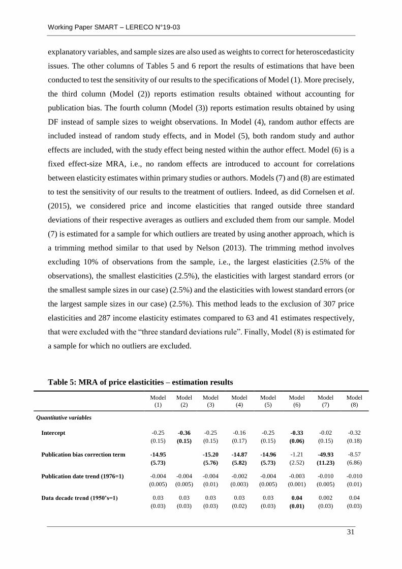
Estimation results are presented in Table 5 for price elasticities and in Table 6 for income
elasticities. In both tables, the second column (Model (1)) reports the estimated coefficient of
our “baseline” mixed effect MRA model. In this model, random primary study effects are
included, publication bias is accounted for by using the inverse primary sample sizes as
Working Paper SMART – LERECO N°19-03
31
explanatory variables, and sample sizes are also used as weights to correct for heteroscedasticity
issues. The other columns of Tables 5 and 6 report the results of estimations that have been
conducted to test the sensitivity of our results to the specifications of Model (1). More precisely,
the third column (Model (2)) reports estimation results obtained without accounting for
publication bias. The fourth column (Model (3)) reports estimation results obtained by using
DF instead of sample sizes to weight observations. In Model (4), random author effects are
included instead of random study effects, and in Model (5), both random study and author
effects are included, with the study effect being nested within the author effect. Model (6) is a
fixed effect-size MRA, i.e., no random effects are introduced to account for correlations
between elasticity estimates within primary studies or authors. Models (7) and (8) are estimated
to test the sensitivity of our results to the treatment of outliers. Indeed, as did Cornelsen et al.
(2015), we considered price and income elasticities that ranged outside three standard
deviations of their respective averages as outliers and excluded them from our sample. Model
(7) is estimated for a sample for which outliers are treated by using another approach, which is
a trimming method similar to that used by Nelson (2013). The trimming method involves
excluding 10% of observations from the sample, i.e., the largest elasticities (2.5% of the
observations), the smallest elasticities (2.5%), the elasticities with largest standard errors (or
the smallest sample sizes in our case) (2.5%) and the elasticities with lowest standard errors (or
the largest sample sizes in our case) (2.5%). This method leads to the exclusion of 307 price
elasticities and 287 income elasticity estimates compared to 63 and 41 estimates respectively,
that were excluded with the “three standard deviations rule”. Finally, Model (8) is estimated for
a sample for which no outliers are excluded.
Table 5: MRA of price elasticities – estimation results
Model
(1)
Model
(2)
Model
(3)
Model
(4)
Model
(5)
Model
(6)
Model
(7)
Model
(8)
Quantitative variables
Intercept -0.25
(0.15)
-0.36
(0.15)
-0.25
(0.15)
-0.16
(0.17)
-0.25
(0.15)
-0.33
(0.06)
-0.02
(0.15)
-0.32
(0.18)
Publication bias correction term -14.95
(5.73) -15.20
(5.76)
-14.87
(5.82)
-14.96
(5.73)
-1.21
(2.52)
-49.93
(11.23)
-8.57
(6.86)
Publication date trend (1976=1) -0.004
(0.005)
-0.004
(0.005)
-0.004
(0.01)
-0.002
(0.003)
-0.004
(0.005)
-0.003
(0.001)
-0.010
(0.005)
-0.010
(0.01)
Data decade trend (1950’s=1) 0.03
(0.03)
0.03
(0.03)
0.03
(0.03)
0.03
(0.02)
0.03
(0.03)
0.04
(0.01)
0.002
(0.03)
0.04
(0.03)

Working Paper SMART – LERECO N°19-03
32
Model
(1)
Model
(2)
Model
(3)
Model
(4)
Model
(5)
Model
(6)
Model
(7)
Model
(8)
GDP per capita (in 1,000 US$) 0.005
(0.0005)
0.005
(0.000)
5)
0.005
(0.0004)
0.005
(0.0005)
0.005
(0.0005)
0.003
(0.0005)
0.005
(0.0004)
0.005
(0.0006)
Household income level
(%age of highest income)
-0.01
(0.02)
-0.01
(0.02)
-0.01
(0.02)
-0.02
(0.02)
-0.01
(0.02)
-0.04
(0.02)
0.02
(0.02)
-0.01
(0.03)
Nominal variables
Type of data
Panel 0.10
(0.16)
0.21
(0.16)
0.10
(0.16)
-0.37
(0.15)
0.10
(0.16)
0.15
(0.06)
0.35
(0.16)
0.07
(0.19)
Cross section 0.13
(0.15)
0.24
(0.15)
0.14
(0.15)
-0.16
(0.15)
0.13
(0.15)
0.23
(0.06)
0.43
(0.15)
0.04
(0.18)
Data level
Individual -0.13
(0.12)
-0.15
(0.12)
-0.13
(0.12)
-0.001
(0.13)
-0.13
(0.12)
-0.21
(0.04)
-0.46
(0.13)
-0.05
(0.15)
Product
Dairy -0.13
(0.01)
-0.13
(0.01)
-0.13
(0.01)
-0.13
(0.01)
-0.13
(0.01)
-0.12
(0.02)
-0.13
(0.01)
-0.09
(0.02)
Fruits and vegetables -0.08
(0.01)
-0.08
(0.01)
-0.08
(0.01)
-0.08
(0.01)
-0.08
(0.01)
-0.09
(0.01)
-0.07
(0.01)
-0.05
(0.02)
Meat and fish -0.10
(0.01)
-0.10
(0.01)
-0.10
(0.01)
-0.10
(0.01)
-0.10
(0.01)
-0.10
(0.01)
-0.09
(0.01)
-0.14
(0.02)
Oils and fats 0.01
(0.02)
0.01
(0.02)
0.01
(0.02)
0.01
(0.02)
0.01
(0.02)
0.02
(0.02)
0.03
(0.01)
0.03
(0.02)
Other food products -0.18
(0.01)
-0.18
(0.01)
-0.18
(0.01)
-0.18
(0.01)
-0.18
(0.01)
-0.18
(0.02)
-0.17
(0.01)
-0.17
(0.02)
Product aggregation level
Product level 0.03
(0.05)
0.03
(0.05)
0.03
(0.05)
-0.04
(0.05)
0.03
(0.05)
-0.09
(0.02)
-0.02
(0.04)
0.01
(0.06)
Region
East Asia -0.02
(0.04)
-0.01
(0.04)
-0.02
(0.04)
-0.005
(0.04)
-0.02
(0.04)
-0.01
(0.03)
-0.02
(0.04)
0.01
(0.05)
Asia Other -0.13
(0.04)
-0.12
(0.04)
-0.13
(0.04)
-0.13
(0.04)
-0.13
(0.04)
-0.21
(0.03)
-0.12
(0.03)
-0.13
(0.05)
European Union -0.04
(0.03)
-0.03
(0.03)
-0.04
(0.03)
-0.03
(0.03)
-0.04
(0.03)
-0.10
(0.02)
-0.03
(0.03)
-0.03
(0.05)
Europe Other -0.10
(0.05)
-0.10
(0.05)
-0.11
(0.05)
-0.10
(0.05)
-0.10
(0.05)
-0.26
(0.04)
-0.11
(0.05)
-0.10
(0.07)
Former Soviet Union -0.11
(0.04)
-0.10
(0.04)
-0.11
(0.04)
-0.11
(0.04)
-0.11
(0.04)
-0.20
(0.03)
-0.10
(0.03)
-0.10
(0.05)

Working Paper SMART – LERECO N°19-03
33
Model
(1)
Model
(2)
Model
(3)
Model
(4)
Model
(5)
Model
(6)
Model
(7)
Model
(8)
Latin America -0.08
(0.04)
-0.07
(0.04)
-0.08
(0.04)
-0.07
(0.04)
-0.08
(0.04)
-0.15
(0.03)
-0.07
(0.03)
-0.07
(0.05)
Middle East -0.09
(0.04)
-0.09
(0.04)
-0.10
(0.04)
-0.09
(0.04)
-0.09
(0.04)
-0.22
(0.03)
-0.09
(0.03)
-0.10
(0.05)
North Africa -0.10
(0.05)
-0.09
(0.05)
-0.10
(0.05)
-0.10
(0.05)
-0.10
(0.05)
-0.19
(0.05)
-0.09
(0.05)
-0.10
(0.07)
Sub-Saharan Africa -0.19
(0.04)
-0.18
(0.04)
-0.19
(0.04)
-0.18
(0.04)
-0.19
(0.04)
-0.28
(0.03)
-0.17
(0.03)
-0.20
(0.05)
Oceania -0.04
(0.05)
-0.03
(0.05)
-0.04
(0.05)
-0.03
(0.05)
-0.04
(0.05)
-0.10
(0.05)
-0.04
(0.04)
-0.03
(0.07)
Urban vs rural households
Urban 0.03
(0.03)
0.03
(0.03)
0.03
(0.03)
0.03
(0.03)
0.03
(0.03)
0.09
(0.02)
0.05
(0.03)
0.03
(0.04)
Rural -0.02
(0.03)
-0.02
(0.03)
-0.02
(0.03)
-0.01
(0.03)
-0.02
(0.03)
0.05
(0.02)
0.01
(0.03)
-0.01
(0.04)
Demand model
AIDS -0.39
(0.13)
-0.36
(0.13)
-0.39
(0.13)
-0.60
(0.15)
-0.39
(0.13)
-0.50
(0.04)
-0.32
(0.12)
-0.41
(0.15)
LAIDS -0.43
(0.13)
-0.40
(0.13)
-0.43
(0.13)
-0.67
(0.15)
-0.43
(0.13)
-0.40
(0.04)
-0.3
(0.11)
-0.44
(0.15)
QUAIDS -0.41
(0.13)
-0.39
(0.13)
-0.41
(0.14)
-0.44
(0.15)
-0.41
(0.14)
-0.44
(0.04)
-0.33
(0.12)
-0.44
(0.16)
Rotterdam -0.38
(0.15)
-0.34
(0.15)
-0.38
(0.15)
-0.61
(0.16)
-0.38
(0.15)
-0.17
(0.07)
-0.22
(0.14)
-0.33
(0.18)
Translog -0.36
(0.16)
-0.43
(0.15)
-0.35
(0.16)
-0.61
(0.17)
-0.36
(0.16)
-0.40
(0.05)
-0.23
(0.15)
-0.36
(0.18)
Single equation -0.55
(0.17)
-0.60
(0.17)
-0.56
(0.17)
-0.60
(0.20)
-0.55
(0.17)
-0.68
(0.05)
-0.96
(0.17)
-0.7
(0.19)
Other -0.32
(0.13)
-0.30
(0.13)
-0.33
(0.13)
-0.56
(0.15)
-0.33
(0.13)
-0.21
(0.04)
-0.35
(0.12)
-0.27
(0.15)
Zero demands accounted for
Yes 0.004
(0.07)
0.02
(0.07)
0.004
(0.07)
0.04
(0.05)
0.004
(0.07)
-0.01
(0.02)
-0.03
(0.06)
-0.04
(0.08)
Prices adjusted for quality
Yes -0.07
(0.06)
-0.07
(0.06)
-0.07
(0.06)
-0.22
(0.05)
-0.07
(0.06)
0.01
(0.03)
-0.09
(0.05)
-0.04
(0.08)
Individuals’ characteristics included
Yes -0.15
(0.08)
-0.11
(0.08)
-0.15
(0.08)
-0.02
(0.05)
-0.15
(0.08)
-0.06
(0.03)
-0.17
(0.07)
-0.04
(0.1)

Working Paper SMART – LERECO N°19-03
34
Model
(1)
Model
(2)
Model
(3)
Model
(4)
Model
(5)
Model
(6)
Model
(7)
Model
(8)
Products’ characteristics included
Yes -0.14
(0.13)
-0.13
(0.13)
-0.14
(0.13)
-0.11
(0.1)
-0.14
(0.13)
-0.12
(0.07)
-0.06
(0.12)
-0.08
(0.15)
Time variables included
Yes -0.07
(0.06)
-0.08
(0.06)
-0.07
(0.06)
-0.10
(0.04)
-0.07
(0.06)
-0.11
(0.02)
-0.02
(0.06)
-0.05
(0.07)
Multi-stage budgeting
Yes 0.04
(0.06)
0.04
(0.06)
0.04
(0.06)
0.002
(0.05)
0.04
(0.06)
0.02
(0.02)
-0.03
(0.05)
0.03
(0.07)
Econometric method
Least Square regression 0.13
(0.10)
0.11
(0.1)
0.13
(0.10)
0.23
(0.10)
0.13
(0.10)
0.29
(0.04)
0.18
(0.10)
0.13
(0.12)
SUR 0.11
(0.07)
0.09
(0.06)
0.11
(0.07)
0.34
(0.06)
0.11
(0.07)
0.17
(0.02)
0.09
(0.06)
0.09
(0.08)
Other 0.08
(0.07)
0.06
(0.07)
0.08
(0.07)
0.20
(0.07)
0.08
(0.07)
0.14
(0.03)
0.17
(0.07)
0.03
(0.09)
Number of observations 3,334 3,334 3,334 3,334 3,334 3,334 3,090 3,397
-2LogLikelihood -329.9 -323.2 -332.6 -308.1 -329.9 62.3 -1093.3 1978.4
Akaike’ Information Criterion -239.9 -235.2 -242.6 -218.1 -237.9 150.3 -1003.3 2068.4
Bayesian Information Criterion -135.1 -132.6 -137.7 -132.0 -130.7 419.3 -902.1 2069.6
Variance of error terms 0.19 0.19 0.19 0.19 0.19 0.23 0.15 0.38
Variance of random effect
Study effect 0.03 0.03 0.03 0.02 - 0.02 0.04
Author effect - - 0.05 0.02 - - -
Note: Standard errors are in parentheses, parameter estimates significant at 5% are reported in bold – Model (1):
“baseline” – Model (2): no correction for publication bias – Model (3): DF used to weight observations – Model
(4): Random author effect – Model (5): Random author effect – Model (6): Fixed effect MRA – Model (7):
Treatment of outliers by trimming method – Model (8): No treatment of outliers.

Working Paper SMART – LERECO N°19-03
35
Table 6: MRA of income elasticities – estimation results
Model
(1)
Model
(2)
Model
(3)
Model
(4)
Model
(5)
Model
(6)
Model
(7)
Model
(8)
Quantitative variables
Intercept 0.41
(0.25)
0.23
(0.23)
0.40
(0.25)
0.35
(0.28)
0.41
(0.25)
0.74
(0.08)
0.13
(0.20)
0.56
(0.27)
Publication bias correction term -24.66
(6.29) -23.78
(6.36)
-31.76
(6.48)
-24.66
(6.29)
-4.67
(3.37)
10.16
(8.14)
-17.73
(8.26)
Publication date trend (1976=1) 0.003
(0.01)
0.01
(0.01)
0.003
(0.01)
0.01
(0.004)
0.003
(0.01)
-0.001
(0.002)
0.01
(0.01)
0.01
(0.01)
Data decade trend (1950’s=1) 0.01
(0.03)
0.01
(0.03)
0.01
(0.03)
-0.03
(0.03)
0.01
(0.03)
0.05
(0.02)
-0.02
(0.03)
-0.04
(0.04)
GDP per capita (in 1,000 US$) -0.01
(0.0005)
-0.01
(0.0005)
-0.01
(0.0005)
-0.01
(0.0005)
-0.01
(0.0005)
-0.01
(0.0005)
-0.01
(0.0005)
-0.01
(0.0005)
Household income level
(%age of highest income)
-0.19
(0.03)
-0.21
(0.03)
-0.19
(0.03)
-0.18
(0.03)
-0.19
(0.03)
-0.21
(0.03)
-0.11
(0.03)
-0.23
(0.04)
Nominal variables
Type of data
Panel -0.25
(0.25)
-0.27
(0.24)
-0.25
(0.25)
0.10
(0.21)
-0.25
(0.25)
-0.52
(0.08)
-0.19
(0.21)
-0.26
(0.28)
Cross section -0.10
(0.21)
-0.11
(0.21)
-0.10
(0.21)
0.29
(0.20)
-0.10
(0.21)
-0.08
(0.07)
-0.12
(0.17)
-0.06
(0.24)
Data level
Individual -0.19
(0.18)
-0.07
(0.17)
-0.18
(0.18)
-0.26
(0.19)
-0.19
(0.18)
0.05
(0.06)
-0.06
(0.15)
-0.11
(0.21)
Product
Dairy 0.29
(0.02)
0.29
(0.02)
0.28
(0.02)
0.28
(0.02)
0.29
(0.02)
0.28
(0.02)
0.26
(0.01)
0.34
(0.03)
Fruits and vegetables 0.15
(0.02)
0.15
(0.02)
0.15
(0.01)
0.15
(0.02)
0.15
(0.02)
0.14
(0.02)
0.14
(0.01)
0.19
(0.02)
Meat and fish 0.28
(0.01)
0.28
(0.01)
0.28
(0.01)
0.27
(0.01)
0.28
(0.01)
0.29
(0.02)
0.25
(0.01)
0.32
(0.02)
Oils and fats 0.05
(0.02)
0.05
(0.02)
0.05
(0.02)
0.05
(0.02)
0.05
(0.02)
0.05
(0.02)
0.03
(0.02)
0.11
(0.03)
Other food products 0.36
(0.02)
0.36
(0.02)
0.36
(0.02)
0.36
(0.02)
0.36
(0.02)
0.34
(0.02)
0.33
(0.01)
0.44
(0.02)
Product aggregation level
Product level 0.07
(0.06)
0.05
(0.06)
0.07
(0.06)
0.11
(0.05)
0.07
(0.06)
-0.06
(0.03)
0.18
(0.05)
-0.01
(0.07)

Working Paper SMART – LERECO N°19-03
36
Model
(1)
Model
(2)
Model
(3)
Model
(4)
Model
(5)
Model
(6)
Model
(7)
Model
(8)
Region
East Asia 0.03
(0.05)
0.03
(0.05)
0.03
(0.05)
-0.005
(0.05)
0.03
(0.05)
-0.01
(0.03)
0.03
(0.04)
0.02
(0.07)
Asia Other 0.15
(0.04)
0.15
(0.04)
0.15
(0.04)
0.13
(0.04)
0.15
(0.04)
-0.07
(0.04)
0.15
(0.04)
0.12
(0.07)
European Union 0.04
(0.04)
0.04
(0.04)
0.04
(0.04)
0.01
(0.04)
0.04
(0.04)
-0.03
(0.03)
0.04
(0.03)
0.02
(0.06)
Europe Other 0.11
(0.06)
0.12
(0.06)
0.11
(0.06)
0.07
(0.05)
0.11
(0.06)
-0.09
(0.04)
0.11
(0.05)
0.09
(0.08)
Former Soviet Union 0.12
(0.04)
0.12
(0.04)
0.12
(0.04)
0.10
(0.04)
0.12
(0.04)
-0.01
(0.04)
0.12
(0.04)
0.10
(0.07)
Latin America 0.09
(0.04)
0.09
(0.04)
0.09
(0.04)
0.07
(0.04)
0.09
(0.04)
-0.02
(0.04)
0.08
(0.04)
0.07
(0.06)
Middle East 0.10
(0.04)
0.11
(0.04)
0.10
(0.04)
0.09
(0.04)
0.10
(0.04)
-0.03
(0.04)
0.10
(0.04)
0.08
(0.06)
North Africa 0.11
(0.06)
0.11
(0.06)
0.11
(0.06)
0.10
(0.06)
0.11
(0.06)
-0.02
(0.06)
0.11
(0.05)
0.09
(0.09)
Sub-Saharan Africa 0.22
(0.04)
0.22
(0.04)
0.22
(0.04)
0.21
(0.04)
0.22
(0.04)
0.09
(0.04)
0.20
(0.04)
0.22
(0.06)
Oceania 0.04
(0.06)
0.04
(0.06)
0.04
(0.06)
0.02
(0.05)
0.04
(0.06)
-0.07
(0.05)
0.03
(0.05)
0.01
(0.08)
Urban vs rural households
Urban -0.08
(0.04)
-0.07
(0.04)
-0.08
(0.04)
-0.13
(0.04)
-0.08
(0.04)
-0.10
(0.03)
-0.09
(0.04)
-0.04
(0.06)
Rural 0.05
(0.04)
0.05
(0.04)
0.05
(0.04)
-0.01
(0.04)
0.05
(0.04)
0.04
(0.03)
-0.004
(0.04)
0.10
(0.06)
Demand model
AIDS 0.27
(0.23)
0.30
(0.22)
0.27
(0.23)
0.10
(0.26)
0.27
(0.23)
0.07
(0.05)
0.36
(0.18)
0.28
(0.24)
LAIDS 0.24
(0.23)
0.26
(0.21)
0.24
(0.23)
0.06
(0.27)
0.24
(0.23)
0.21
(0.05)
0.31
(0.18)
0.27
(0.24)
QUAIDS 0.28
(0.23)
0.30
(0.21)
0.28
(0.22)
0.09
(0.26)
0.28
(0.23)
-0.02
(0.05)
0.31
(0.18)
0.23
(0.24)
Rotterdam 0.19
(0.24)
0.21
(0.23)
0.19
(0.24)
0.11
(0.28)
0.19
(0.24)
-0.28
(0.08)
0.10
(0.20)
0.12
(0.27)
Translog 0.74
(0.26)
0.59
(0.24)
0.74
(0.26)
0.78
(0.28)
0.74
(0.26)
0.39
(0.07)
0.76
(0.21)
0.68
(0.28)
Single equation -0.04
(0.26)
0.04
(0.25)
-0.04
(0.26)
-0.38
(0.32)
-0.04
(0.26)
0.03
(0.06)
0.13
(0.21)
-0.03
(0.28)

Working Paper SMART – LERECO N°19-03
37
Model
(1)
Model
(2)
Model
(3)
Model
(4)
Model
(5)
Model
(6)
Model
(7)
Model
(8)
Other 0.14
(0.23)
0.19
(0.22)
0.15
(0.23)
-0.11
(0.27)
0.14
(0.23)
-0.16
(0.06)
0.30
(0.18)
0.12
(0.25)
Zero demands accounted for
Yes -0.18
(0.10)
-0.15
(0.10)
-0.18
(0.1)
-0.19
(0.07)
-0.18
(0.10)
-0.28
(0.02)
-0.14
(0.09)
-0.21
(0.11)
Prices adjusted for quality
Yes 0.14
(0.12)
0.16
(0.11)
0.14
(0.12)
-0.05
(0.06)
0.14
(0.12)
0.04
(0.03)
0.15
(0.09)
0.14
(0.12)
Individuals’ characteristics included
Yes 0.12
(0.11)
0.17
(0.11)
0.12
(0.11)
-0.11
(0.08)
0.12
(0.11)
-0.01
(0.03)
0.17
(0.09)
0.15
(0.12)
Products’ characteristics included
Yes )0.22
(0.19)
0.26
(0.19)
0.23
(0.19)
0.35
(0.16)
0.22
(0.19)
0.27
(0.09)
0.12
(0.15)
0.71
(0.21)
Time variables included
Yes 0.01
(0.09)
0.001
(0.09)
0.01
(0.09)
0.0007
(0.06)
0.01
(0.09)
0.02
(0.02)
-0.02
(0.07)
0.01
(0.10)
Multi-stage budgeting
Yes -0.20
(0.09)
-0.19
(0.09)
-0.2
(0.09)
-0.37
(0.07)
-0.20
(0.09)
-0.27
(0.03)
-0.21
(0.08)
-0.20
(0.10)
Econometric method
Least Square regression 0.08
(0.13)
0.04
(0.13)
0.07
(0.13)
0.46
(0.14)
0.08
(0.13)
-0.25
(0.04)
0.03
(0.12)
0.03
(0.16)
SUR 0.06
(0.1)
0.02
(0.10)
0.06
(0.10)
0.48
(0.09)
0.06
(0.10)
-0.09
(0.03)
0.04
(0.08)
0.02
(0.11)
Other 0.06
(0.12)
-0.02
(0.11)
0.06
(0.12)
0.48
(0.1)
0.06
(0.12)
0.02
(0.04)
-0.01
(0.1)
0.05
(0.13)
Number of observations 3,311 3,311 3,311 3,311 3,311 3,311 3,065 3,352
-2LogLikelihood 511.9 526.9 494.7 495.6 511.9 1220.3 -624.5 3287.2
Akaike’ Information Criterion 601.9 614.9 584.7 585.6 603.9 1308.3 -534.5 3377.9
Bayesian Information Criterion 703.1 713.9 685.9 673.4 707.4 1576.9 -438.8 3479.1
Variance of error terms 0.23 0.24 0.23 0.23 0.23 0.31 0.17 0.54

Working Paper SMART – LERECO N°19-03
38
Model
(1)
Model
(2)
Model
(3)
Model
(4)
Model
(5)
Model
(6)
Model
(7)
Model
(8)
Variance of random effect
Study effect 0.07 0.06 0.07 - 0.03 - 0.04 0.07
Author effect - - - 0.12 0.03 -
Note: Standard errors are in parentheses, parameter estimates significant at 5% are reported in bold – Model (1):
“baseline” – Model (2): no correction for publication bias – Model (3): DF used to weight observations – Model
(4): Random author effect – Model (5): Random author effect – Model (6): Fixed effect MRA – Model (7):
Treatment of outliers by trimming method – Model (8): No treatment of outliers.
Several findings from the estimation results of Model (1) shown in Tables 5 and 6 can be
highlighted.
First, GDP per capita has a significant and negative impact on income elasticities and a positive
impact on uncompensated price elasticities, meaning that both elasticities decrease in absolute
terms with GDP per capita. Household income level also has a significant and negative impact
on income elasticities within countries, which confirms the relevance of using this information
rather than considering average elasticities computed across all household income levels, as in
Cornelsen et al. (2015). The decrease in income elasticities with income levels is indeed in
accordance with economic theory related to Engel’s law (see, e.g., Pinstrup-Andersen and
Caicedo (1978), who highlight this point). It is also not surprising that food demand becomes
less responsive to price as incomes increase (see, e.g., Alderman, 1986), especially for
uncompensated price elasticities that by definition incorporate income effects of price changes
(Clements et al., 2006). These results are also in line with the food demand elasticities estimates
provided in Seale et al. (2003a) and Muhammad et al. (2011), who undertake an international
comparison of food consumption patterns.
Second, the type of product involved has a significant impact on income and price elasticities:
income elasticities tend to be lowest for cereals, higher for oils and fats and fruits and
vegetables, and the highest for meat and dairy products. The ranking is the same for price
elasticities. Once again, these results appear to be in accordance with the theory, and are in line
with those of Seale et al. (2003a) and Muhammad et al. (2011), who found that for individual
countries, staple food demand is less responsive to price and income than luxury food demand.
Third, some patterns emerge from the regional parameter estimates. Indeed, world regions
appear to be divided into two groups. For a first group of regions (the EU, East Asia, North

Working Paper SMART – LERECO N°19-03
39
Africa and Oceania), the estimated “region” coefficients are not significantly different from
zero in our meta-regressions, implying that in these regions’ elasticities (income or price) are
similar to those of the reference region, North America. In the second group of regions (Sub-
Saharan Africa, Latin America, the Middle East, the Former Soviet Union, other European
countries and other Asian countries), income and price elasticities tend to be higher in absolute
terms than in the reference region. Since GDP per capita is controlled for in the estimation
procedure, this result might be attributed to other differences between developed (the first
group) and developing countries (the second group). These differences could, for instance, be
related to differences in the diversification of consumption baskets tastes or to differences in
tastes across countries as shown by Clements et al. (2006) through their comparison of
international consumption patterns for broad product categories.
Fourth, turning to the characteristics related to the specification of the model and method used
to estimate demand elasticities, the main effect on estimated elasticity values observed appears
to be related to the model used to represent demand. Price elasticity estimates derived from
flexible forms, such as the AIDS of quadratic or linear form and from Rotterdam and Translog
demand systems, appear significantly higher than those derived from the LES and CES and
lower than those derived from ad hoc single equations. This result stands in contrast with the
conclusions of Cornelsen et al. (2016), who find no significant effects of the functional form
used to estimate food demand price elasticities. However, these authors only distinguish AIDS
and “non-AIDS” forms of demand systems. On the other hand, they find estimation methods to
have a significant impact on estimated elasticities, which is not found to be the case in our study
for the same classification of estimation methods. Their result might in fact be related to effects
of the functional form used to estimate elasticities, as the selection of an estimation method
generally results from the specification of the econometric model to be estimated. Functional
forms appear to have less impact on estimated income elasticities with only the Translog
demand system having an impact on these elasticities that is significantly different from other
functional forms. However, while adopting a multi-stage budgeting framework is found to have
no significant impact on price elasticity estimates, it appears to lead to significantly lower
income elasticities, and this is the case, although we only consider unconditional income
elasticities. This shows that methodological strategies influence the value of estimated
elasticities and calls for sensitivity analyses from economists using estimated elasticities in their
models.
All conclusions regarding the effects of income, products, regions, functional forms and multi-
stage budgeting remain valid when we consider different MRA model specifications (Models

Working Paper SMART – LERECO N°19-03
40
(2)-(6)) or sample selection methods (Models (7)-(8)). According to the Aikaike and Bayesian
Information Criteria (AIC and BIC) reported at the end of Tables 5 and 6, the specification
including a correction of publication bias (Model (1)) is preferred to the specification without
this correction (Model (2)), which was expected. Furthermore, among the different
specifications used to account for unobserved heterogeneity and potential correlations between
elasticity estimates (random study effects in Model (1), random author effects in Model (4),
both types of effects in Model (5) and no effect in Model (6)) 8, the model including random
study effects appears to be the preferred one. Most of the differences in estimation results
actually appear with the fixed effect-size MRA model (Model (6)), where several explanatory
variables that are found, in Model (1), to have no significant impact on elasticity estimates, such
as the decade a dataset refers to, the type of data concerned, the levels of product aggregation
or the distinctions between urban and rural households, appear to be significant in Model (6).
As is shown by Bateman and Jones (2003), not accounting for the heterogeneity between studies
that remains after observable study characteristics are taken into account can lead to misleading
conclusions regarding the impacts of several of these characteristics on price and income
elasticity estimates.
5. Conclusion
The main purposes of this paper were twofold: first, to reveal general patterns characterizing
the demand elasticities of food products and second, to identify the major sources of
heterogeneity between the estimates of the elasticities available in the literature to help
economists to select empirical estimates of these key parameters for their simulation models.
To achieve these objectives, we conducted a broad literature review of food demand elasticity
estimates and performed an MRA. The MRA applied herein differs from those of previous
works addressing similar issues in several respects. First, we considered not only price but also
income elasticity, which can have considerable impacts on the outcomes of simulation models.
Second, relative to previous studies, additional variables characterizing elasticity estimates
were included in our analysis. We notably considered more detailed categorizations of
functional forms representing food demand and information on household income levels. Third,
8 Models (3), (6), (7) and (8) are not directly comparable to the other specifications since they are not estimated
based on the same data. In Model (3), a different variable is used to weight observations, and Model (7) and (8)
are estimated based on different samples of observations.

Working Paper SMART – LERECO N°19-03
41
in line with the MAER-NET protocol, heteroscedasticity issues were accounted for and
publication selection bias was addressed, and we relied on a mixed-effect MRA model to
account for potential correlations between elasticity estimates collected from the same study.
Our results first reveal some general patterns regarding the levels of price and income
elasticities of food demand elasticities. We found demand to be less responsive to income and
price changes for staple products, which conforms to economic theory. It also appears that
income levels have important impacts on income and price elasticities both at country (GDP)
and household levels: the higher the income is, the lower the level of elasticity. We also found
demand elasticities to present different patterns depending on the global region considered apart
from any income level considerations.
Beyond these factual elements and perhaps more importantly, the functional forms used to
represent food demand were found to significantly affect price elasticity estimates, and the
adoption of multi-stage budgeting frameworks was found to significantly impact unconditional
income elasticity estimates. These results contrast with those obtained through previous meta-
analysis and can notably be attributed to the more thorough representation of the modelling
food demand considered here. Our results show that methodological strategies influence the
value of estimated elasticities and call for sensitivity analyses from economists using estimated
food demand elasticities to calibrate their models. This is all the more important because food
demand elasticities are crucial parameters in the calibration of simulation models used to assess
the impacts of agricultural policy reforms.
Sensitivity analyses were performed to test the robustness of our results to the specifications of
the MRA models. Our main results proved to be robust to the assumptions underlying these
models.
Finally, it should be noted that the meta-analysis presented here does not consider potential
differences in food elasticities between domestic and imported goods. This is because the
primary studies included in our dataset do not provide sufficient information for analysing this
issue, as none of them distinguish between imported and domestic goods. This is, however, an
important question since, as shown by Seale et al. (2003b), for example, in the case of wine in
the US, income and price elasticities can significantly differ between domestic and imported
goods and between different sources of imported goods. Notably, this can have important
implications when using elasticities to calibrate models aimed at simulating the impacts of trade
policies. This point should be considered in future work analysing food demand elasticity
estimates.
Working Paper SMART – LERECO N°19-03
42
References
Alderman, H. (1986). The effect of food price and income changes on the acquisition of food
by low-income households. International Food Policy Research Institute, 100 p.
Andreyeva, T., Long, M.W., Brownell, K.D. (2010). The impact of food prices on consumption:
a systematic review of research on the price elasticity of demand for food. American Journal
of Public Health, 100(2): 216-222.
Banks, J., Blundell, R., Lewbel, A. (1997). Quadratic Engel curves and consumer demand.
Review of Economics and Statistics, 79(4): 527-539.
Barten, A.P. (1964). Consumer demand functions under conditions of almost additive
preferences. Econometrica: Journal of the Econometric Society, 32(1-2): 1-38.
Bateman, I.J., Jones, A.P. (2003). Contrasting conventional with multi-level modeling
approaches to meta-analysis: expectation consistency in UK woodland recreation values.
Land Economics, 79(2): 235-258.
Borenstein, M., Hedges, L.V., Higgins, J., Rothstein, H.R. (2010). A basic introduction to
Fixed‐effect and random‐effects models for meta‐analysis. Research Synthesis Methods,
1(2): 97-111.
Carpentier, A., Gohin, A., Sckokai, P., Thomas, A. (2015). Economic modelling of agricultural
production: past advances and new challenges. Revue d’Études en Agriculture et
Environnement, 96(1): 131-165.
Carpentier, A., Guyomard, H. (2001). Unconditional elasticities in two-stage demand systems:
an approximate solution. American Journal of Agricultural Economics, 83(1): 222-229.
Chen, D., Abler, D., Zhou, D., Yu, X., Thompson, W. (2016). A meta-analysis of food demand
elasticities for China. Applied Economic Perspectives and Policy, 38(1): 50-72.
Christensen, L.R., Jorgenson, D.W., Lau, L.J. (1975). Transcendental logarithmic utility
functions. The American Economic Review, 65(3): 367-383.
Cipollina M., Salvatici, L. (2010). Reciprocal trade agreements in gravity models: a meta-
analysis. Review of International Economics, 18(1): 63-80.
Clarke, L., Edmonds, J., Jacoby, H., Pitcher, H., Reilly, J., Richels, R. (2007). Scenarios of
greenhouse gas emissions and atmospheric concentrations. US Department of Energy
Publications, 116 p. Available at
https://science.energy.gov/~/media/ber/pdf/Sap_2_1a_final_all.pdf.

Working Paper SMART – LERECO N°19-03
43
Clements, K.W., Gao, G. (2015). The Rotterdam demand model half a century on. Economic
Modelling, 49: 91-103.
Clements, K.W., Wu, Y., Zhang, J. (2006). Comparing international consumption patterns.
Empirical Economics, 31(1): 1-30.
Cornelsen, L., Green, R., Turner, R., Dangour, A.D., Shankar, B., Mazzocchi, M., Smith, R.D.
(2015). What Happens to Patterns of Food Consumption when Food Prices Change?
Evidence from A Systematic Review and Meta‐Analysis of Food Price Elasticities Globally.
Health Economics, 24(12): 1548-1559.
Cornelsen, L., Mazzocchi, M., Green, R., Dangour, A.D., Smith, R.D. (2016). Estimating the
Relationship between Food Prices and Food Consumption-Methods Matter. Applied
Economic Perspectives and Policy, 38(3): 546-561.
Day, B. (1999). A meta-analysis of wage-risk estimates of the value of statistical life. EC,
Benefits transfer and the economic valuation of environmental damages. European
Commission, Brussels, 29 p. Available at
http://citeseerx.ist.psu.edu/viewdoc/download?doi=10.1.1.550.7320&rep=rep1&type=pdf
Deaton, A. (1988). Quality, quantity, and spatial variation of price. The American Economic
Review, 78(3): 418-430.
Deaton, A., Muellbauer, J. (1980). An almost ideal demand system. The American economic
review, 70(3): 312-326.
Disdier, A.C., Head, K. (2008). The puzzling persistence of the distance effect on bilateral trade.
The Review of Economics and Statistics, 90(1): 37-48.
Eales, J.S., Unnevehr, L.J. (1988). Demand for beef and chicken products: separability and
structural change. American Journal of Agricultural Economics, 70(3): 521-532.
Edgerton, D.L. (1997). Weak separability and the estimation of elasticities in multistage
demand systems. American Journal of Agricultural Economics, 79(1): 62-79.
Egger, M., Smith, G.D., Schneider, M., Minder, C. (1997). Bias in meta-analysis detected by a
simple, graphical test. Bristish Medical Journal, 315(7109): 629-634.
Fabiosa, J.F., Jensen, H.H. (2003). Usefulness of incomplete demand model in censored demand
system estimation. Paper prepared for Presentation at the 2003 Annual meeting, July 27-30,
Montreal, Canada, No. 21923. American Agricultural Economics Association (New Name
2008: Agricultural and Applied Economics Association). Canada.

Working Paper SMART – LERECO N°19-03
44
Fang, C., Beghin, J.C. (2002). Urban demand for edible oils and fats in China: Evidence from
household survey data. Journal of Comparative Economics, 30(4): 732-753.
Fogarty, J. (2010). The demand for beer, wine and spirits: A survey of the literature. Journal of
Economic Surveys, 24(3): 428-478.
Gallet, C. (2010). The income elasticity of meat: a meta-analysis. The Australian Journal of
Agricultural and Resource Economics, 54(4): 477-490.
Gallet, C. (2008). Meat meets meta: A quantitative review of the price elasticity of meat.
American Journal of Agricultural Economics, 92(1): 258-272.
Gould, B.W. (1996): Factors affecting US demand for reduced-fat fluid milk. Journal of
Agricultural and Resource Economics, 21 (1): 68-81.
Green, R., Cornelsen, L., Dangour, A.D., Turner, R., Shankar, B., Mazzocchi, M., Smith, R.D.
(2013). The effect of rising food prices on food consumption: systematic review with meta-
regression. British Medical Journal, 346: f3703.
Hahn, W.F. (2001). Maximum likelihood estimation of a random coefficient meat demand
system. Paper prepared for Presentation at the 2001 Summer Meetings of the American
Agricultural Economics Association, Chicago, IL, 19 p. Available at
https://ageconsearch.umn.edu/record/20573/files/sp01ha02.pdf
Han, T., Cramer, G.L. Wahl, T.I. (1997): Rural household food consumption in China:
evidence from the Rural Household Survey. Paper prepared for Presentation at the 1997
WAEA Meeting July 13-16, Reno, NY.
Havlík, P., Schneider, U.A., Schmid, E., Böttcher, H., Fritz, S., Skalsky, R., Aoki, K., De Cara,
S., Kindermann, G., Kraxner, F., Leduc, S., McCallum, I. Mosnier, A., Sauer, T.,
Obersteiner, M. (2011). Global land-use implications of first and second generation biofuel
targets. Energy Policy, 39(10): 5690-5702.
Heien, D., Wessels, C.R. (1990). Demand systems estimation with microdata: a censored
regression approach. Journal of Business and Economic Statistics, 8(3): 365-371.
Higgins, J.P., Thompson, S.G. (2002). Quantifying heterogeneity in a meta‐analysis. Statistics
in Medicine, 21(11): 1539-1558.
Huang, K.S., Lin, B.H. (2000). Estimation of food demand and nutrient elasticities from
household survey data. Washington, DC: US Department of Agriculture, Economic

Working Paper SMART – LERECO N°19-03
45
Research Service. Technical Bulletin No. 1887, 24 p. Available at
https://core.ac.uk/download/pdf/7083123.pdf
Keller, W.J., Van Driel, J. (1985). Differential consumer demand systems. European Economic
Review, 27(3): 375-390.
Laborde, D., Valin, H. (2012). Modeling land-use changes in a global CGE: assessing the EU
biofuel mandates with the MIRAGE-BioF model. Climate Change Economics, 3 (3):
1250017.
Lee, L.F., Pitt, M.M. (1986). Microeconometric demand system with binding nonnegativity
constraints: the dual approach. Econometrica: Journal of the Econometric Society, 54(5):
1237-1242.
Melo, P.C., Abdul-Salam, Y., Roberts, D., Gilbert, A., Matthews, R., Colen, L., Mary, S., Y
Paloma, S.G (2015). Income elasticities of food demand in Africa: A meta-analysis. JRC
Technical report. European Commission. Sevilla. Spain, 74 p. Available at
http://publications.jrc.ec.europa.eu/repository/bitstream/JRC98812/jrc98812_jrc_report_m
eta_analysis_final.pdf
Moschini, G. (1999). Imposing local curvature conditions in flexible demand systems. Journal
of Business and Economic Statistics, 17(4): 487-490.
Moschini, G. (1998). The semiflexible almost ideal demand system. European Economic
Review, 42(2): 349-364.
Muhammad, A., Seale, J.L., Meade, B., Regmi, A. (2011). International Evidence on Food
Consumption Patterns: An Update Using 2005 International Comparison Program Data.
USDA-ERS Technical Bulletin No. 1929, 59 p. Available at
https://core.ac.uk/download/pdf/6718963.pdf
Nelson, J.P. (2013a). Meta-analysis of Alcohol Price and Income Elasticities – With
Corrections for Publication Bias. Health Economics Review, 3(1): 17.
Nelson, J.P. (2013b). Robust demand elasticities for wine and distilled spirits: Meta-Analysis
with corrections for outliers and publication bias. Journal of Wine Economics, 8(3): 294-
317.
Nelson, J.P., Kennedy, P.E. (2009). The use (and abuse) of meta-analysis in environmental and
natural resource economics: an assessment. Environmental and Resource Economics, 42(3):
345-377.

Working Paper SMART – LERECO N°19-03
46
Neves, P.D. (1994). A class of differential demand systems. Economics Letters, 44(1-2): 83-
86.
Ogundari, K., Abdulai, A. (2013). Examining the Heterogeneity in Calorie-income elasticities:
A Meta-analysis. Food Policy, 40(6): 119-128.
Pinstrup-Andersen, P, Caicedo, E. (1978). The potential impact of changes in income
distribution on food demand and human nutrition. American Journal of Agricultural
Economics, 60(3): 402-415.
Roberts, C.J. (2005). Issues in meta‐regression analysis: an overview. Journal of Economic
Surveys, 19(3): 295-298.
Robinson, S., Mason d'Croz, D., Islam, S., Sulser, T.B., Robertson, R.D., Zhu, T., Gueneau, A.,
Pitois, G., Rosegrant, M.W. (2015). The International Model for Policy Analysis of
Agricultural Commodities and Trade (IMPACT): Model description for version 3. IFPRI
Discussion Paper 1483. Washington, D.C, 55 p. Available at
http://ebrary.ifpri.org/utils/getfile/collection/p15738coll2/id/127162/filename/127373.pdf
Rude, J.I., Meilke, K.D. (2004). Developing policy relevant agrifood models. Journal of
Agricultural and Applied Economics, 36(2): 369-382.
Ryan, D. L., Wales, T.J. (1998). A simple method for imposing local curvature in some flexible
consumer-demand systems. Journal of Business & Economic Statistics, 16(3): 331-338.
Sam, A.G., Zheng, Y. (2010). Semiparametric estimation of consumer demand systems with
micro data. American Journal of Agricultural Economic, 92(1): 246-257.
Santeramo, F.G., Shabnam, N. (2015). The income-elasticity of calories, macro-and micro-
nutrients: What is the literature telling us? Food Research International, 76(4): 932-937.
Schafgans, M.M.A. (2004). Finite Sample Properties for the Semiparametric Estimation of the
Intercept of a Censored Regression Model. Statistica Neerlandica, 58(1): 35-56.
Seale, J.L., Regmi, A., Bernstein, J. (2003a). International evidence on food consumption
patterns. USDA Technical Bulletin No. TB-1904. 70 p. Available at
https://ageconsearch.umn.edu/record/33580/files/tb031904.pdf.
Seale, J.L., Marchant, M.A., Basso, A. (2003b). Imports versus domestic production: A demand
system analysis of the US red wine market. Review of Agricultural Economics, 25(1): 187-
202.

Working Paper SMART – LERECO N°19-03
47
Selvanathan, S., Selvanathan, E.A. (1993). A cross-country analysis of consumption patterns.
Applied Economics, 25(9): 1245-1259.
Seo, S.C. and O. Capps (1997): Regional variability of price and expenditure elasitcities: The
case of spaghetti sauces. Agribusiness, 13 (6): 659-672.
Shonkwiler, J.S., Yen, S.T. (1999). Two-step estimation of a censored system of equations.
American Journal of Agricultural Economics, 81(4): 972-982.
Sornpaisarn, B., Shield, K., Cohen, J., Schwartz, R., Rehm, J. (2013). Elasticity of Alcohol
Consumption, Alcohol-related Harms, and Drinking Initiation in Low- and Middle-Income
Countries: A Systematic Review and Meta-analysis. International Journal of Alcohol and
Drug Research, 2(1): 45-58.
Stanley, T.D. (2008). Meta‐regression methods for detecting and estimating empirical effects
in the presence of publication selection. Oxford Bulletin of Economics and Statistics, 70(1):
103-127.
Stanley, T.D. (2005). Beyond publication bias. Journal of Economic Surveys, 19(3): 309-345.
Stanley, T.D., Doucouliagos, H. (2014). Meta-regression approximations to reduce publication
selection bias. Research Synthesis Methods, 5(1): 60-78.
Stanley, T.D., Doucouliagos, H., Giles, M., Heckemeyer, J.H., Johnston, R.J, Laroche, P.,
Nelson, J.P., Paldam, M., Poot, J., Pugh, G., Rosenberger, R.S., Rost, K. (2013). Meta-
Analysis of Economic Research Reporting Guidelines. Journal of Economic Surveys, 27(2):
390-394.
Stanley, T.D., Jarrell, S.B. (1989). Meta‐regression analysis: a quantitative method of literature
surveys. Journal of Economic Surveys, 3(2): 161-170.
Sutton, A., Duval, S., Tweedie, R., Abrams, K., Jones, D. (2000). Empirical Assessment of
effect of publication bias on meta-analyses. British Medical Journal, 320(7249): 1574-1577.
Timmer, C.P., Falcon, W.P., Pearson, S.R. (1983). Food policy analysis. World Bank/Johns
Hopkins Johns Hopkins University Press. Baltimore, 301 p.
Theil, H. (1965). The information approach to demand analysis. Econometrica: Journal of the
Econometric Society, 33(1): 67-87.
Tyers, R., Anderson, K. (1992). Disarray in world food markets. Cambridge Books, 284 p.

Working Paper SMART – LERECO N°19-03
48
USDA. (2005). Commodity and food elasticities. Accessed May 2015. Available at
https://www.ers.usda.gov/data-products/commodity-and-food-elasticities/
Valin, H. , Sands, R.D., van der Mensbrugghe, D. , Nelson, G.C., Ahammad, H. , Blanc, E. ,
Bodirsky, B. , Fujimori, S. , Hasegawa, T. , Havlik, P. , Heyhoe, E. , Kyle, P. , Mason‐
D'Croz, D. , Paltsev, S. , Rolinski, S. , Tabeau, A. , van Meijl, H. , von Lampe, M.,
Willenbockel, D. (2014). The future of food demand: understanding differences in global
economic models. Agricultural Economics, 45(1): 51-67.
Wagenaar A.C., Salois M.J., Komro, K.A. (2009). Effects of beverage alcohol price and tax
levels on drinking: a meta-analysis of 1003 estimates from 112 studies. Addiction, 104(2):
179-190.
Wales, T.J., Woodland, A.D. (1983). Estimation of consumer demand systems with binding
non-negativity constraints. Journal of Econometrics, 21(3): 263-285.
Yen, S.T., Lin, B.H., Smallwood, D.M. (2003). Quasi-and simulated-likelihood approaches to
censored demand systems: food consumption by food stamp recipients in the United States.
American Journal of Agricultural Economics, 85(2): 458-478.
Yu, W., Hertel, T.W., Preckel, P.V., Eales, J.S. (2004). Projecting world food demand using
alternative demand systems. Economic Modelling, 21(1): 99-129.

Working Paper SMART – LERECO N°19-03
49
Appendix 1: primary studies included in the database
Provision of food demand elasticities for a complete set of food products
Abdulai, A. (2002): Household demand for food in Switzerland. A quadratic almost ideal
demand system, Swiss Journal of Economics and Statistics 138 (1): 1-122.
Abdulai, A. and D. Aubert (2004): A cross-section analysis of household demand for food and
nutrients in Tanzania, Agricultural economics 31 (1): 67-79.
Abdulai, A., Jain, D.K. and A.K. Sharma (1999): Household food demand analysis in India,
Journal of agricultural economics 50 (2): 316-327.
Agbola, F.F. (2003): Estimation of food demand patterns in South Africa based on a survey of
households, Journal of Agricultural and Applied Economics 35 (3): 663-682.
Akbay, C., Boz, I. and W.S. Chern (2007): Household food consumption in Turkey, European
Review of Agricultural Economics 34 (2): 209-231.
Alfonzo, L. and H.H. Peterson (2006): Estimating food demand in Paraguay from household
survey data, Agricultural Economics 34 (3): 243-257.
Balisacan, A.M. (1994): Demand for food in the Philippines: responses to price and income
changes, Philippine Review of Economics and Business 31 (2): 137-163.
Burney, N.A. and M. Akmal (1991): Food demand in Pakistan: An application of the extended
linear expenditure system, Journal of agricultural economics 42 (2): 185-195.
Cupak, A., Pokrivcak, J., Rizov, M., Alexandri, C. and L. Luca (2014): Economic development
and food demand in Central and Eastern European countries: The case of Romania. Paper
prepared for Presentation at the 142nd European Association of Agricultural Economists
Seminar, May 29-30, 2014, Budapest, Hungary.
Durham, C. and J. Eales (2006): Demand elasticities for fresh fruit at the retail level. Selected
Paper prepared for presentation at the American Agricultural Economics Association
Annual Meeting, Long Beach, July 23-26, 2006, California.
Ecker, O. and M. Qaim (2008): Income and price elasticities of food demand and nutrient
consumption in Malawi. Paper prepared for Presentation at the American Agricultural
Economics Association Annual Meeting, July 27-29, 2008, Orlando, FL.

Working Paper SMART – LERECO N°19-03
50
Fan, S., Cramer, G. and E. Wailes (1994): Food demand in rural China: evidence from rural
household survey, Agricultural Economics 11 (1): 61-69.
Fan, S., Wailes, E.J. and G.L. Cramer (1995): Household demand in rural China: a two-stage
LES-AIDS model, American Journal of Agricultural Economics 77 (1): 54-62.
Gao, X.M., Wailes, E.J. and G.L. Cramer (1996): A two-stage rural household demand analysis:
Microdata evidence from Jiangsu Province, China, American Journal of Agricultural
Economics 78 (3): 604-613.
Gould, B.W. (2002): Household composition and food expenditures in China, Agribusiness 18
(3): 387-407.
Gould, B.W. and D. Dong (2004): Product quality and the demand for food: the case of urban
China. Paper prepared for Presentation at the Annual meeting, American Agricultural
Economics Association (New Name 2008: Agricultural and Applied Economics
Association) August 1-4, Denver, CO (No. 20010).
Guo, X., Popkin, B.M., Mroz, T.A. and F. Zhai (1999): Food price policy can favorably alter
macronutrient intake in China, The Journal of Nutrition 129 (5): 994-1001.
Han, T., Cramer, G.L. and T.I. Wahl (1997): Rural household food consumption in China:
evidence from the Rural Household Survey. Paper prepared for Presentation at the 1997
WAEA Meeting July 13-16, Reno, NY.
Huang, J. and S. Rozelle (1998): Market development and food demand in rural China, China
Economic Review 9 (1): 25-45.
Huang, K.S. (1985): US demand for food: A complete system of price and income effects.
Washington, DC: US Department of Agriculture, Economic Research Service. Technical
bulletin 1714.
Huang, K.S. and B.H. Lin (2000): Estimation of food demand and nutrient elasticities from
household survey data. Washington, DC: US Department of Agriculture, Economic
Research Service. Technical Bulletin No. 1887.
Jensen, H.H. and J. Manrique (1998): Demand for food commodities by income groups in
Indonesia, Applied Economics 30 (4): 491-501.
Kumar, P., Kumar A., Parappurathu, S. and S.S. Raju (2011): Estimation of demand elasticity
for food commodities in India, Agricultural Economics Research Review 24 (1): 1-14.

Working Paper SMART – LERECO N°19-03
51
Liu, K.E. and W.S. Chern (2003): Food demand in urban China: an application of a multi-stage
censored demand system. Paper prepared for Presentation at the Annual Meeting of the
American Agricultural Economic Association, Montreal, Canada. 27-30.
Mergos, G.J. and G.S. Donatos (1989): Demand for food in Greece: An almost ideal demand
system analysis, Journal of Agricultural Economics 40 (2): 178-184.
Mhurchu N.C., Eyles H., Schilling C., Yang Q., Kaye-Blake W., Genç M and T. Blakely
(2013): Food prices and consumer demand: differences across income levels and ethnic
groups, PLoS ONE 8(10): e75934.
Min, I., Fang, C. and Q. Li (2004): Investigation of patterns in food-away-from-home
expenditure for China, China Economic Review 15 (4): 457-476.
Mittal, S. (2006): Structural shift in demand for food: Projections for 2020. ICRIER Working
Paper. 184
Molina, J.-A. (1994): Food demand in Spain: An application of the almost ideal system, Journal
of Agricultural Economics 45 (2): 252-258.
Muhammad, A. Seale, J.L., Meade, B. and A. Regmi (2011): International Evidence on Food
Consumption Patterns: An Update Using 2005 International Comparison Program Data.
USDA-ERS Technical Bulletin No. 1929.
Pitt, M.M. (1983): Food preferences and nutrition in rural Bangladesh, The Review of
Economics and Statistics 65 (1): 105-114.
Rickertsen, K. (1998): The demand for food and beverages in Norway, Agricultural economics
18 (1): 89-100.
Sahn, D.E. (1988): The effect of price and income changes on food-energy intake in Sri Lanka,
Economic Development and Cultural Change 36 (2): 315-340.
Seale, J.L., Regmi, A. and J. Bernstein (2003): International evidence on food consumption
patterns. USDA Technical Bulletin No. TB-1904. 70.
Shono, C., Suzuki, N. and H.M. Kaiser (2000): Will China's diet follow western diets?
Agribusiness 16 (3): 271-279.
Tiffin, A. and R. Tiffin (1999): Estimates of food demand elasticities for Great Britain: 1972–
1994, Journal of Agricultural Economics 50 (1): 140-147.

Working Paper SMART – LERECO N°19-03
52
Udoh, E.J., Mbossoh, E.R., Udoh, E.S. and S.B. Akpan (2013): The structure of food demand
in urban city of Nigeria: An application of a Linearized Almost Ideal Demand System
(LA/AIDS)], Journal of Development and Agricultural Economics 5 (1): 12-18.
Yan, W. and W.S. Chern (2005): Estimating food demand in rural China under the perspectives
of agricultural household models. Paper prepared for Presentation at the American
Agricultural Economics Association Annual Meeting, Providence, Rhode Island, USA.
http://ageconsearch. umn. edu/bitstream/19171/1/sp05ya02. pdf.
Yen, S.T., Fang, C. and S.J. Su (2004): Household food demand in urban China: a censored
system approach, Journal of Comparative Economics 32 (3): 564-585.
Zhang, W. and Q. Wang (2003): Changes in China’s urban food consumption and implications
for trade. Paper prepared for Presentation at the American Agricultural Economics
Association annual meeting, July. Montreal, Canada. 27-30.
Zhang, X., Mount, T.D. and R.N Boisvert. (2001): The demand for food grain in China: New
insights into a controversy, Agricultural and Resource Economics Review 30 (1): 1-9.
Provision of food demand elasticities for one food sector
Crutchfield, S.R. (1985): An econometric model of the market for New England groundfish,
Northeast Journal of Agricultural and Resource Economics 14: 128-143.
Fang, C. and J.C. Beghin (2002): Urban demand for edible oils and fats in China: Evidence
from household survey data, Journal of Comparative Economics 30 (4): 732-753.
Fulponi, L. (1989): The almost ideal demand system: An application to food and meat groups
for France, Journal of Agricultural Economics 40 (1): 82-92.
Gallet, C.A. and J.A. List (1998): Elasticities of beer demand revisited, Economics Letters 61
(1): 67-71.
Gould, B.W. (1996): Factors affecting US demand for reduced-fat fluid milk, Journal of
Agricultural and Resource Economics 21 (1): 68-81.
Gould, B.W., Cox, T.L. and F. Perali (1991): Demand for food fats and oils: the role of
demographic variables and government donations, American Journal of Agricultural
Economics 73 (1): 212-221.

Working Paper SMART – LERECO N°19-03
53
Han, T. and T.I. Wahl (1998): China's rural household demand for fruit and vegetables, Journal
of Agricultural and Applied Economics 30: 141-150.
Han, T., Wahl, T.I. and R.C. Mittelhammer (1998): Rural household fruit and vegetable
consumption in China. Paper prepared for Presentation at the 1998 Annual meeting,
American Agricultural Economics Association (New Name 2008: Agricultural and
Applied Economics Association) August 2-5, Salt Lake City, UT (No. 20854).
Heien, D. and G. Pompelli (1988): The demand for beef products: cross-section estimation of
demographic and economic effects, Western Journal of Agricultural Economics 13 (1): 37-
44.
Helen, D. and L.S. Willett, (1986): The demand for sweet spreads demographic and economic
effects for detailed commodities, Northeastern Journal of Agricultural and Resource
Economics 15 (2): 160-167.
Jabarin, A.S. (2005): Estimation of meat demand system in Jordan: an almost ideal demand
system, International Journal of consumer studies 29 (3): 232-238.
Lee, J.Y., Brown, M.G. and J.L. Seale (1992): Demand relationships among fresh fruit and
juices in Canada, Review of Agricultural Economics 14 (2): 255-262.
Lusk, J.L., Marsh, T.L., Schroeder, T.C. and J.A. Fox (2001): Wholesale demand for USDA
quality graded boxed beef and effects of seasonality, Journal of Agricultural and Resource
Economics 26 (1): 91-106.
Ma, H., Huang, J., Rozelle, S. and A. Rae (2003): Livestock product consumption patterns in
urban and rural china. Center for Applied Economics and Policy Studies, Massey
University. China Agriculture Working Paper, 1-25.
Menkhaus, D.J., St. Clair, J.S. and S. Hallingbye (1985): A reexamination of consumer buying
behavior for beef, pork, and chicken, Western Journal of Agricultural Economics 10 (1):
116-125.
Mergenthaler, M., Weinberger, K. and M. Qaim (2009): The food system transformation in
developing countries: A disaggregate demand analysis for fruits and vegetables in Vietnam,
Food Policy 34 (5): 426-436.
Niu, L. and M. Wohlgenant (2012): A censored demand system analysis of fruits and vegetables
by different income groups using micro data. Paper prepared for Presentation at the
Working Paper SMART – LERECO N°19-03
54
Agricultural and Applied Economics Association’s 2012 AAEA Annual Meeting, August
12-14, 2012. Seattle, Washington.
Thompson, G.D. and P.N. Wilson (1999): Market demands for bagged, refrigerated salads,
Journal of Agricultural and Resource Economics 24 (2):463-481.
Tiffin, R. and M. Aguiar (1995): Bayesian estimation of an almost ideal demand system for
fresh fruit in Portugal, European review of agricultural economics 22 (4): 469-480.
Wadud, Md. A. (2006): An analysis of meat demand in Bangladesh using the almost ideal
demand system, The Empirical Economics Letters 5 (1): 29-35.
Wang, Q., Fuller, F., Hayes, D. and C. Halbrendt (1998): Chinese consumer demand for animal
products and implications for US pork and poultry exports, Journal of Agricultural and
Applied Economics 30 (1): 127-140.
Wang, Q., Halbrendt, C.C. and H.H. Jensen (1997): China's beer consumption and barley
imports, Agribusiness 13 (1): 73-84.
Yen, S.T. and C.L. Huang (2002): Cross-sectional estimation of US demand for beef products:
a censored system approach, Journal of Agricultural and Resource Economics 27 (2): 320-
334.
Yen, S.T., Kan, K. and S.J. Su (2002): Household demand for fats and oils: two-step estimation
of a censored demand system, Applied Economics 34 (14): 1799-1806.
Yen, S.T., Lin, B.H., Harris, J.M. and N. Ballenger (2004): Demand for differentiated
vegetables. Paper prepared for Presentation at the American Agricultural Economics
Association Annual Meeting, August. Denver, Colorado. 1-4.
You, Z., Epperson, J.E. and C.L. Huang (1996): A composite system demand analysis for fresh
fruits and vegetables in the United States, Journal of Food Distribution Research 27 (3):
11-22.
Study of the impacts of advertising on the structure of food demand
Capps, O., Seo, S.C. and J.P. Nichols (1997): On the estimation of advertising effects for
branded products: An application to spaghetti sauces, Journal of Agricultural and Applied
Economics 29 (2): 291-302.

Working Paper SMART – LERECO N°19-03
55
Kinnucan, H.W., Miao, Y., Xiao, H. and H.M. Kaiser (2001): Effects of advertising on US non-
alcoholic beverage demand: Evidence from a two-stage Rotterdam model. In Michael R.
Baye, Jon P. Nelson (ed.) Advertising and Differentiated Products (Advances in Applied
Microeconomics, Volume 10) Emerald Group Publishing Limited.1-29.
Richards, T.J., Gao, X.M. and P.M. Patterson (1999): Advertising and retail promotion of
Washington apples: a structural latent variable approach to promotion evaluation, Journal
of Agricultural and Applied Economics 31 (1): 15-28.
Schmit, T.M., Dong, D., Chung, C., Kaiser, H.M. and B.W. Gould (2002): Identifying the
effects of generic advertising on the household demand for fluid milk and cheese: a two-
step panel data approach, Journal of Agricultural and Resource Economics 27 (1): 165-
186.
Study of the impacts of product differentiation on the structure of food demand
Adelaja, A.O., Brumfield, R.G. and K. Lininger (1990): Product differentiation and state
promotion of farm produce: An analysis of the Jersey Fresh tomato, Journal of Food
Distribution Research 21 (3): 73-86.
Foxall, G.R, Yan, J., Oliveira-Castro, J.M. and V.K. Wells (2013): Brand-related and situational
influences on demand elasticity, Journal of Business Research 66 (1): 73-81.
Glaser, L.K. and G.D. Thompson (2000): Demand for organic and conventional beverage milk.
Paper prepared for Presentation at the Western Agricultural Economics Association
Annual Meeting, June. Vancouver. British Columbia.
Glaser, L.K. and G.D. Thompson (1998): Demand for organic and conventional frozen
vegetables. Paper prepared for Presentation at the Annual Meeting, No 21583, 1999 Annual
meeting American Agricultural Economics Association, August 8-11, Nashville, TN.
Gould, B.W. and H.J. Villarreal (2006): An assessment of the current structure of food demand
in urban China, Agricultural Economics 34 (1): 1-16.
Study of the impacts of health policies on the structure of food demand
Flake, O. and P.M. Patterson (1999): Health, Food Safety and Meat Demand. Paper prepared
for Presentation at the AAEA Annual Meetings, August 1999, Nashville, TN.

Working Paper SMART – LERECO N°19-03
56
Henneberry, S.R., Piewthongngam, K. and H. Qiang (1999): Consumer food safety concerns
and fresh produce consumption, Journal of Agricultural and Resource Economics 24(1):
98-113.
Kinnucan, H.W., Xiao, H., Hisa, C.-J. and J.D. Jackson (1997): Effects of health information
and generic advertising on US meat demand, American Journal of Agricultural Economics
79 (1): 13-23.
Piggott, N.E. and T.L. Marsh (2004): Does food safety information impact US meat demand?
American Journal of Agricultural Economics 86 (1):154-174.
Smed, S., Jensen, J.D. and S. Denver (2007): Socio-economic characteristics and the effect of
taxation as a health policy instrument, Food Policy 32 (5): 624-639.
Verbeke, W. and R.W. Ward (2001): A fresh meat almost ideal demand system incorporating
negative TV press and advertising impact, Agricultural Economics 25 (2-3): 359-374.
Study of the impacts of structural changes on the structure of food demand
Ahmadi-Esfahani, F.Z. and R.G. Stanmore (1997): Demand for vegetables in a Chinese
wholesale market, Agribusiness 13 (5): 549-559.
Attanasio, O., Di Maro, V., Lechene, V. and P. David (2013): Welfare consequences of food
prices increases: Evidence from rural Mexico, Journal of Development Economics 104:
136-151.
Dahlgran, R.A. (1987): Complete flexibility systems and the stationarity of US meat demands,
Western Journal of Agricultural Economics 12 (2): 152-163.
Haq, Z., Nazli, H. and K. Meilke (2008): Implications of high food prices for poverty in
Pakistan, Agricultural Economics 39 (1): 477-484.
Huang, J. and H. Bouis (2001): Structural changes in the demand for food in Asia: empirical
evidence from Taiwan, Agricultural Economics 26 (1): 57-69.
Moschini, G. and K.D. Meilke (1989): Modeling the pattern of structural change in US meat
demand, American journal of agricultural economics 71(2): 253-261.
Pinstrup-Andersen, P. and E. Caicedo (1978): The potential impact of changes in income
distribution on food demand and human nutrition, American Journal of Agricultural
Economics 60 (3): 402-415.

Working Paper SMART – LERECO N°19-03
57
Ulimwengu, J.M., Workneh, S. and Z. Paulos (2009): Impact of soaring food price in Ethiopia:
Does location matter? IFPRI Discussion Paper 00846.
Wood, B.D.K., Nelson, C.H. and L. Nogueira (2012): Poverty effects of food price escalation:
The importance of substitution effects in Mexican households, Food policy 37 (1): 77-85.
Zheng, Z. and S.R. Henneberry (2010): The impact of changes in income distribution on current
and future food demand in urban China, Journal of Agricultural and Resource Economics
35 (1): 51-71.
Methodological focus: functional forms of demand models or econometric estimation
procedures
Alston, J.M. and J.A. Chalfant (1993): The silence of the lambdas: A test of the almost ideal
and Rotterdam models, American journal of agricultural economics 75 (2): 304-313.
Balcombe, K.G. and J.R. Davis (1996): An application of cointegration theory in the estimation
of the almost ideal demand system for food consumption in Bulgaria, Agricultural
Economics 15 (1): 47-60.
Banks, J., Blundell, R. and A. Lewbel (1997): Quadratic Engel curves and consumer demand,
Review of Economics and statistics 79 (4): 527-539.
Bergtold, J., Akobundu, E. and E. B. Peterson (2004): The FAST method: Estimating
unconditional demand elasticities for processed foods in the presence of fixed effects,
Journal of Agricultural and Resource Economics 29 (2): 276-295.
Blanciforti, L. and R. Green (1983): An almost ideal demand system incorporating habits: an
analysis of expenditures on food and aggregate commodity groups, The Review of
Economics and Statistics 65 (3): 511-515.
Blundell, R., Pashardes, P. and G. Weber (1993): What do we learn about consumer demand
patterns from micro data? The American Economic Review 83 (3): 570-597.
Bouis, H.E. (1996): A food demand system based on demand for characteristics: if there is
‘Curvature’in the Slutsky Matrix, what do the Curves look like and why? Journal of
Development Economics 51 (2): 239-266.
Brester, G.W. and M.K. Wohlgenant (1993): Correcting for measurement error in food demand
estimation, The Review of Economics and Statistics 75 (2): 352-356.

Working Paper SMART – LERECO N°19-03
58
Brown, M.G. (1986): The demand for fruit juices: market participation and quantity demanded,
Western Journal of Agricultural Economics 11 (2): 179-183.
Brown, M.G. and J.Y. Lee (2000): A uniform substitute demand model with varying
coefficients, Journal of agricultural and applied economics 32 (1): 1-10.
Bryant, H.L. and G.C. Davis (2001): Beyond the Model Specification Problem: Model and
Parameter Averaging Using Bayesian Techniques. In AAEA annual meeting, Chicago, IL:
5-8.
Capps, O. (1989): Utilizing scanner data to estimate retail demand functions for meat products,
American Journal of Agricultural Economics 71 (3): 750-760.
Carpentier, A. and H. Guyomard (2001): Unconditional elasticities in two-stage demand
systems: an approximate solution, American Journal of Agricultural Economics 83 (1):
222-229.
Chen, K.Z. (1998): The symmetric problem in the linear almost ideal demand system,
Economics Letters 59 (3): 309-315.
Cox, T.L. and M.K. Wohlgenant (1986): Prices and quality effects in cross-sectional demand
analysis, American Journal of Agricultural Economics 68 (4): 908-919.
Cox, T.L., Ziemer, R.F. and J.P. Chavas (1984): Household demand for fresh potatoes: A
disaggregated cross-sectional analysis, Western Journal of Agricultural Economics 9 (1):
41-57.
Deaton, A. (1990): Price elasticities from survey data: extensions and Indonesian results,
Journal of Econometrics 44 (3): 281-309.
Deaton, A. (1989): Household survey data and pricing policies in developing countries, The
World Bank Economic Review 3 (2): 183-210.
Dong, D., Gould, B.W. and H.M. Kaiser (2004): Food demand in Mexico: an application of the
Amemiya-Tobin approach to the estimation of a censored food system, American Journal
of Agricultural Economics 86 (4): 1094-1107.
Edgerton, D.L. (1997): Weak separability and the estimation of elasticities in multistage
demand systems, American Journal of Agricultural Economics 79 (1): 62-79.
Fabiosa, J.F. and H.H. Jensen (2003): Usefulness of incomplete demand model in censored
demand system estimation. Paper prepared for Presentation at the 2003 Annual meeting,
Working Paper SMART – LERECO N°19-03
59
July 27-30, Montreal, Canada, No. 21923. American Agricultural Economics Association
(New Name 2008: Agricultural and Applied Economics Association). Canada.
Golan, A., Perloff, J.M. and E.Z. Shen (2001): Estimating a demand system with nonnegativity
constraints: Mexican meat demand, Review of Economics and Statistics 83 (3): 541-550.
Green, R. and J.M. Alston (1990): Elasticities in AIDS models, American Journal of
Agricultural Economics 72 (2): 442-445.
Hahn, W.F. (2001): Maximum likelihood estimation of a random coefficient meat demand
system. Paper prepared for Presentation at the 2001 Summer Meetings of the American
Agricultural Economics Association, Chicago, IL.
Heien, D. and C.R. Wesseils (1990): Demand systems estimation with microdata: a censored
regression approach, Journal of Business and Economic Statistics 8 (3): 365-371.
Heien, D. (1982): The structure of food demand: Interreslatedness and duality, American
Journal of Agricultural Economics 64 (2): 213-221.
Huang, K.S. and R.C. Haidacher (1983): Estimation of a composite food demand system for
the United States, Journal of Business and Economic Statistics 4 (1): 285-291.
Karagiannis, G., Katranidis, S. and K. Velentzas (2000): An error correction almost ideal
demand system for meat in Greece, Agricultural Economics 22 (1): 29-35.
Kastens, T.L. and G.W. Brester (1996): Model selection and forecasting ability of theory-
constrained food demand systems, American Journal of Agricultural Economics 78 (2):
301-312.
Kasteridis, P., Yen, S.T. and C. Fang (2011): Bayesian estimation of a censored linear almost
ideal demand system: Food demand in Pakistan, American Journal of Agricultural
Economics 93 (5): 1374-1390.
Katchova, A.L. and W.S. Chern (2004): Comparison of quadratic expenditure system and
almost ideal demand system based on empirical data, International Journal of Applied
Economics 1 (1): 55-64.
Manser, M.E. (1976): Elasticities of demand for food: an analysis using non-additive utility
functions allowing for habit formation, Southern Economic Journal 43 (1): 879-891.
Meyerhoefer, C.D., Ranney, C.K. and D.E. Sahn (2005): Consistent estimation of censored
demand systems using panel data, American Journal of Agricultural Economics 87 (3):
660-672.

Working Paper SMART – LERECO N°19-03
60
Moschini, G., Moro, D. and R.D. Green (1994): Maintaining and testing separability in demand
systems, American Journal of Agricultural Economics 76 (1): 61-73.
Okrent, A.M. and J.M. Alston (2010): Demand for food in the United States: A review of
literature, evaluation of previous estimates, and presentation of new estimates of demand.
Poster prepared for presentation at the Agricultural and Applied Economics Association
2010 AAEA, CAES, and WAEA Joint Annual Meeting, July 25-27, 2010. Denver,
Colorado.
Park, J.L., Holcomb, R.B., Raper, K.C. and O. Capps (1996): A demand systems analysis of
food commodities by US households segmented by income, American Journal of
Agricultural Economics 78 (2): 290-300.
Pashardes, P. (1993): Bias in estimating the almost ideal demand system with the stone index
approximation, The Economic Journal 103 (419): 908-915.
Price, D.W. and R.C. Mittelhammer (1979): A matrix of demand elasticities for fresh fruits,
Western Journal of Agricultural Economics 4 (01): 69-86.
Reed, A.J., Levedahl J.W. and C. Hallahan (2005): The generalized composite commodity
theorem and food demand estimation, American Journal of Agricultural Economics 87 (1):
28-37.
Seo, S.C. and O. Capps (1997): Regional variability of price and expenditure elasitcities: The
case of spaghetti sauces, Agribusiness 13 (6): 659-672.
Shi, H., Mittelhammer, R. and T.I. Wahl (1995): Aggregate food demand analysis for a
transitional economy: an application to Chinese household expenditure data, Journal of
Food Distribution Research 26 (02): 20-27.
Timmer, C P. and H. Alderman (1979): Estimating consumption parameters for food policy
analysis, American Journal of Agricultural Economics 61 (5): 982-987.
Wohlgenant, M.K. (1989): Demand for farm output in a complete system of demand functions,
American Journal of Agricultural Economics 71 (2): 241-252.
Wohlgenant, M.K. (1985): Estimating cross elasticities of demand for beef, Western Journal of
Agricultural Economics 10 (2):322-329.
Yen, S.T. and B.H. Lin (2006): A sample selection approach to censored demand systems,
American Journal of Agricultural Economics 88 (3): 742-749.

Working Paper SMART – LERECO N°19-03
61
Yen, S.T., Lin, B.H. and D.M. Smallwood (2003): Quasi-and simulated-likelihood approaches
to censored demand systems: food consumption by food stamp recipients in the United
States, American Journal of Agricultural Economics 85 (2): 458-478.
Yu, W., Hertel, T.W., Preckel, P.V. and J.S. Eales (2004): Projecting world food demand using
alternative demand systems, Economic Modelling 21 (1): 99-129.

Working Paper SMART – LERECO N°19-03
62
Appendix 2. Products mapping
Product name in primary study Product category Aggregation level
apple fruits and
vegetables product level
apricot fruits and
vegetables product level
aquatic product meat aggregate
asparagus fruits and
vegetables product level
baked bean other food products product level
banana fruits and
vegetables product level
barley cereals product level
bean fruits and
vegetables product level
bean and product fruits and
vegetables product level
beef meat product level
beef and mutton meat product level
beef and veal meat product level
biscuits other food products product level
bread other food products product level
bread and cereals cereals aggregate
brown bread other food products product level
butter dairy products product level
cabbage fruits and
vegetables product level
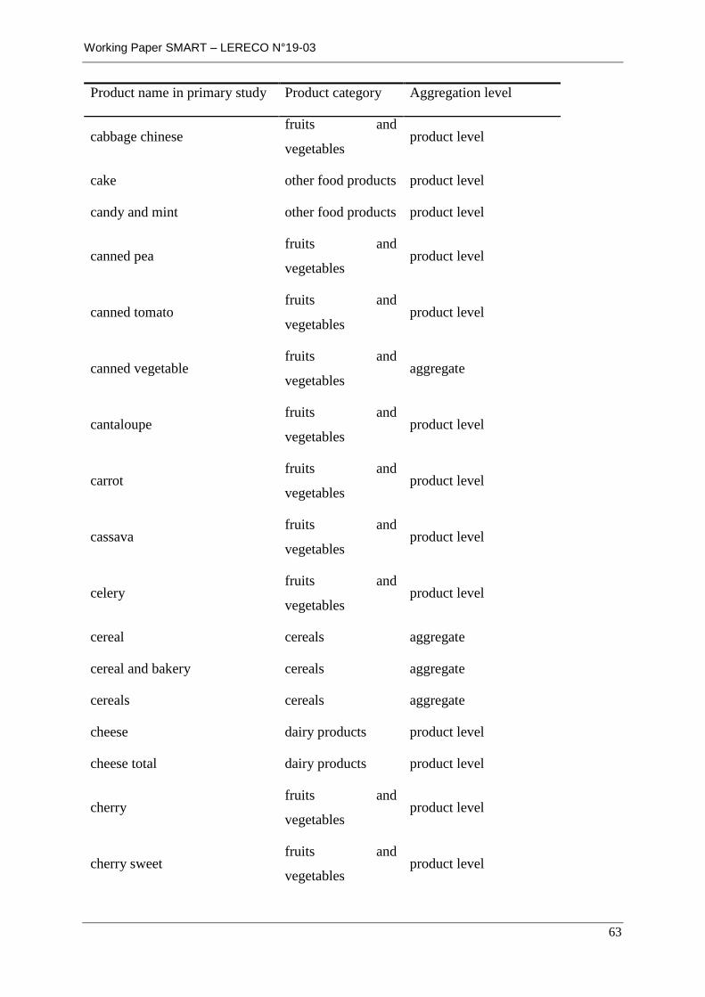
Working Paper SMART – LERECO N°19-03
63
Product name in primary study Product category Aggregation level
cabbage chinese fruits and
vegetables product level
cake other food products product level
candy and mint other food products product level
canned pea fruits and
vegetables product level
canned tomato fruits and
vegetables product level
canned vegetable fruits and
vegetables aggregate
cantaloupe fruits and
vegetables product level
carrot fruits and
vegetables product level
cassava fruits and
vegetables product level
celery fruits and
vegetables product level
cereal cereals aggregate
cereal and bakery cereals aggregate
cereals cereals aggregate
cheese dairy products product level
cheese total dairy products product level
cherry fruits and
vegetables product level
cherry sweet fruits and
vegetables product level

Working Paper SMART – LERECO N°19-03
64
Product name in primary study Product category Aggregation level
chicken meat product level
chive fruits and
vegetables product level
chocolate other food products product level
citrus fruits and
vegetables product level
citrus fruit fruits and
vegetables product level
coarse grain cereals aggregate
cocoa mix and milk flavored other food products product level
coconut fruits and
vegetables product level
corn cereals product level
crucifer fruits and
vegetables product level
cucumber fruits and
vegetables product level
dairy dairy products aggregate
dairy product dairy products aggregate
dairy product and egg other food products aggregate
dried bean fruits and
vegetables product level
dried fruit fruits and
vegetables aggregate
dried vegetable fruits and
vegetables aggregate
egg other food products product level
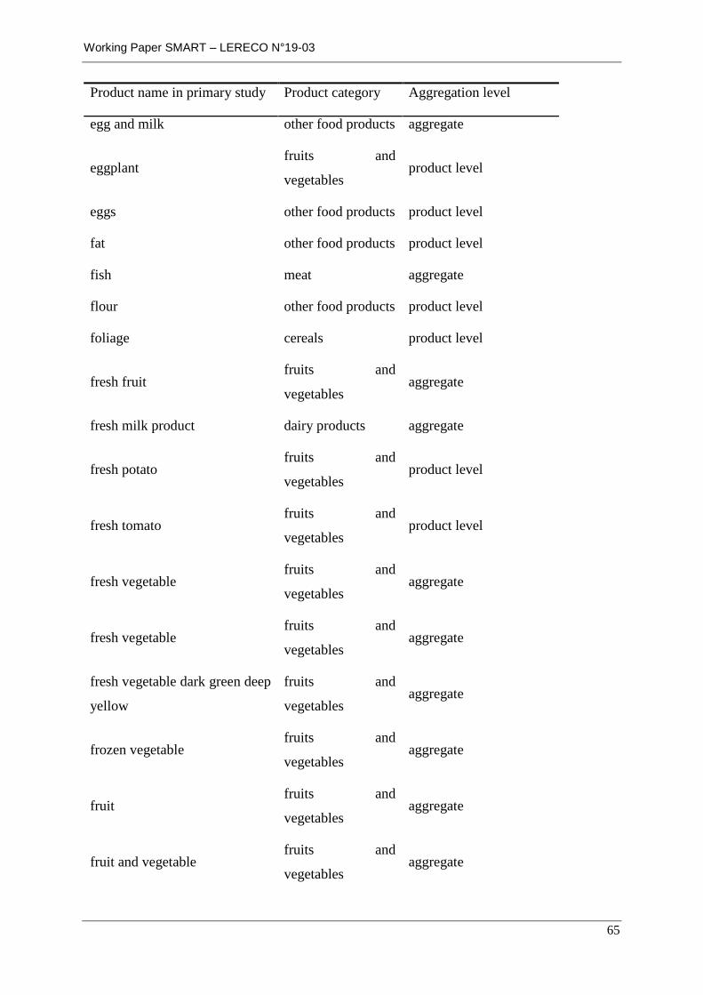
Working Paper SMART – LERECO N°19-03
65
Product name in primary study Product category Aggregation level
egg and milk other food products aggregate
eggplant fruits and
vegetables product level
eggs other food products product level
fat other food products product level
fish meat aggregate
flour other food products product level
foliage cereals product level
fresh fruit fruits and
vegetables aggregate
fresh milk product dairy products aggregate
fresh potato fruits and
vegetables product level
fresh tomato fruits and
vegetables product level
fresh vegetable fruits and
vegetables aggregate
fresh vegetable fruits and
vegetables aggregate
fresh vegetable dark green deep
yellow
fruits and
vegetables aggregate
frozen vegetable fruits and
vegetables aggregate
fruit fruits and
vegetables aggregate
fruit and vegetable fruits and
vegetables aggregate

Working Paper SMART – LERECO N°19-03
66
Product name in primary study Product category Aggregation level
fruit shelf stable fruits and
vegetables aggregate
fruits fruits and
vegetables aggregate
garlic fruits and
vegetables product level
gelatin pudding mix other food products product level
ginger fruits and
vegetables product level
grain cereals aggregate
grain and cereal cereals aggregate
grain food cereals aggregate
grape fruits and
vegetables product level
grapefruit fruits and
vegetables product level
green pepper fruits and
vegetables product level
green vegetable fruits and
vegetables product level
groundnuts fruits and
vegetables product level
honey other food products product level
Ice cream yogurt dairy products product level
icecream dairy products product level
Icecream yogurt dairy products product level
jam other food products product level
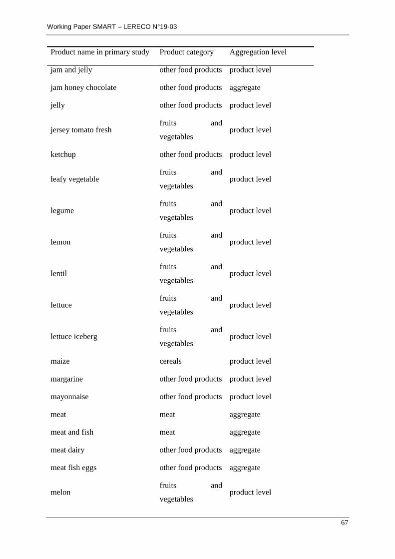
Working Paper SMART – LERECO N°19-03
67
Product name in primary study Product category Aggregation level
jam and jelly other food products product level
jam honey chocolate other food products aggregate
jelly other food products product level
jersey tomato fresh fruits and
vegetables product level
ketchup other food products product level
leafy vegetable fruits and
vegetables product level
legume fruits and
vegetables product level
lemon fruits and
vegetables product level
lentil fruits and
vegetables product level
lettuce fruits and
vegetables product level
lettuce iceberg fruits and
vegetables product level
maize cereals product level
margarine other food products product level
mayonnaise other food products product level
meat meat aggregate
meat and fish meat aggregate
meat dairy other food products aggregate
meat fish eggs other food products aggregate
melon fruits and
vegetables product level

Working Paper SMART – LERECO N°19-03
68
Product name in primary study Product category Aggregation level
milk dairy products product level
milk and dairy products dairy products aggregate
milk cheese and eggs other food products aggregate
milk powder dairy products product level
mix other food products product level
molasses other food products product level
muffin and roll other food products product level
mutton meat product level
mutton and lamb meat product level
nectarine fruits and
vegetables product level
non beef meat product level
Non pork meat product level
Non poultry meat product level
Nut fruits and
vegetables product level
nut snack other food products product level
oil other food products product level
oil and fat other food products product level
oil cooking other food products product level
oil edible other food products product level
oilandfat other food products product level
oilcooking other food products product level
oils and fats other food products product level
oilseed other food products product level

Working Paper SMART – LERECO N°19-03
69
Product name in primary study Product category Aggregation level
onion fruits and
vegetables product level
onion dry fruits and
vegetables product level
onion spring fruits and
vegetables product level
onions fruits and
vegetables product level
onionspring fruits and
vegetables product level
orange fruits and
vegetables product level
other cereals cereals aggregate
other chicken meat product level
other fat other food products product level
other fresh fruit fruits and
vegetables aggregate
other fresh vegetable fruits and
vegetables aggregate
other fresh vegetable fruits and
vegetables aggregate
other fruit fruits and
vegetables aggregate
other fruit fruits and
vegetables aggregate
other grain cereals aggregate
other meat meat product level

Working Paper SMART – LERECO N°19-03
70
Product name in primary study Product category Aggregation level
other milk dairy products product level
other milk product dairy products aggregate
other processed vegetable fruits and
vegetables product level
other tomato fruits and
vegetables product level
other vegetable fruits and
vegetables aggregate
pasta other food products product level
pea fruits and
vegetables product level
peach fruits and
vegetables product level
peanut butter other food products product level
peanut oil other food products product level
pear fruits and
vegetables product level
peasandsoybean fruits and
vegetables product level
pepper fruits and
vegetables product level
pepper green fruits and
vegetables product level
plum fruits and
vegetables product level
popcorn other food products product level
pork meat product level

Working Paper SMART – LERECO N°19-03
71
Product name in primary study Product category Aggregation level
pork other meat product level
potato fruits and
vegetables product level
potatoes fruits and
vegetables product level
poultry meat product level
poultry and fish meat aggregate
processed cereal cereals aggregate
processed fruit fruits and
vegetables aggregate
processed meat meat aggregate
processed potato fruits and
vegetables product level
processed vegetable fruits and
vegetables aggregate
processed vegetable dark green
deep yellow
fruits and
vegetables aggregate
processed wheat cereals
prune and plum fruits and
vegetables product level
pulse fruits and
vegetables product level
pulses fruits and
vegetables product level
pumpkins fruits and
vegetables product level
rapeseed oil other food products product level

Working Paper SMART – LERECO N°19-03
72
Product name in primary study Product category Aggregation level
red meat meat product level
rice cereals product level
root fruits and
vegetables product level
roots fruits and
vegetables product level
salad dressing other food products product level
saladbagged fruits and
vegetables product level
sauce and marinade other food products product level
seafood meat aggregate
seasoning preservative other food products product level
shortening other food products product level
sorghum cereals product level
sour cream dairy products product level
sourcream dairy products product level
soy oil other food products product level
soybean other food products product level
spaghetti sauce other food products product level
spices fruits and
vegetables product level
strawberry fruits and
vegetables product level
sugar other food products product level
sugarnadsweets other food products product level
sweet other food products product level

Working Paper SMART – LERECO N°19-03
73
Product name in primary study Product category Aggregation level
sweetener other food products product level
syrup other food products product level
tangerine fruits and
vegetables product level
tofu other food products product level
tomato fruits and
vegetables product level
tomato fresh fruits and
vegetables product level
tomato processed fruits and
vegetables product level
tuber fruits and
vegetables product level
turkey meat product level
veal meat product level
vegetable fruits and
vegetables aggregate
vegetable oil other food products product level
vegetable root fruits and
vegetables product level
vegetable shelf stable fruits and
vegetables aggregate
vegetables fruits and
vegetables aggregate
vegetables and fruits fruits and
vegetables aggregate

Working Paper SMART – LERECO N°19-03
74
Product name in primary study Product category Aggregation level
watermelon fruits and
vegetables product level
wheat cereals product level
white bread other food products product level
white meat meat product level
yogurt dairy products product level

Working Paper SMART – LERECO N°19-03
75
Appendix 3. Mapping between countries codes and world regions
Country name ISO3 code Region
Afghanistan AFG Other Asian Albania ALB Former Soviet Union
Algeria DZA North Africa American Samoa ASM Oceania
Andorra AND European Union
Angola AGO Sub-Saharan Africa Anguilla AIA Latin America
Antigua and Barbuda ATG Latin America Argentina ARG Latin America
Armenia ARM Former Soviet Union Aruba ABW Latin America
Australia AUS Oceania
Austria AUT European Union Azerbaijan AZE Former Soviet Union
Bahamas, The BHS Latin America Bahrain BHR Middle East
Bangladesh BGD Other Asian
Barbados BRB Latin America Belarus BLR Former Soviet Union
Belgium BEL European Union Belize BLZ Latin America
Benin BEN Sub-Saharan Africa
Bermuda BMU Latin America Bhutan BTN Other Asian
Bolivia BOL Latin America Bosnia and Herzegovina BIH Former Soviet Union
Botswana BWA Sub-Saharan Africa Brazil BRA Latin America
British Virgin Islands VGB Latin America
Brunei BRN Other Asian Bulgaria BGR European Union
Burkina Faso BFA Sub-Saharan Africa Burundi BDI Sub-Saharan Africa
Cambodia KHM Other Asian
Cameroon CMR Sub-Saharan Africa Canada CAN North America
Cape Verde CPV Sub-Saharan Africa Cayman Islands CYM Latin America
Central African Republic CAF Sub-Saharan Africa Chad TCD Sub-Saharan Africa
Chile CHL Latin America
China CHN AsiaEast Christmas Island CXR Other Asian
Cocos (Keeling) Islands CCK Other Asian Colombia COL Latin America
Comoros COM Sub-Saharan Africa
Congo, Republic of the COG Sub-Saharan Africa Cook Islands COK Oceania
Costa Rica CRI Latin America Cote d'Ivoire CIV Sub-Saharan Africa
Croatia HRV Former Soviet Union Cuba CUB Latin America
Cyprus CYP European Union
Czech Republic CZE European Union Denmark DNK European Union
Djibouti DJI Sub-Saharan Africa Dominica DMA Latin America
Dominican Republic DOM Latin America

Working Paper SMART – LERECO N°19-03
76
Country name ISO3 code Region
Ecuador ECU Latin America
Egypt EGY Middle East El Salvador SLV Latin America
Equatorial Guinea GNQ Sub-Saharan Africa
Eritrea ERI Sub-Saharan Africa Estonia EST European Union
Ethiopia ETH Sub-Saharan Africa Falkland Islands (Islas Malvinas) FLK Latin America
Faroe Islands FRO Other European Fiji FJI Oceania
Finland FIN European Union
France FRA European Union French Guiana GUF Latin America
French Polynesia PYF Oceania Gabon GAB Sub-Saharan Africa
Gambia, The GMB Sub-Saharan Africa
Georgia GEO Former Soviet Union Germany DEU European Union
Ghana GHA Sub-Saharan Africa Gibraltar GIB Other European
Greece GRC European Union Greenland GRL North America
Grenada GRD Latin America
Guadeloupe GLP Latin America Guam GUM Oceania
Guatemala GTM Latin America Guernsey -- European Union
Guinea GIN Sub-Saharan Africa
Guinea-Bissau GNB Sub-Saharan Africa Guyana GUY Latin America
Haiti HTI Latin America Holy See (Vatican City) VAT Other European
Honduras HND Latin America Hungary HUN European Union
Iceland ISL Other European
India IND Other Asian Indonesia IDN Other Asian
Iran IRN Middle East Iraq IRQ Middle East
Ireland IRL European Union
Israel ISR Middle East Italy ITA European Union
Jamaica JAM Latin America Jan Mayen -- Other European
Japan JPN AsiaEast Jersey -- European Union
Jordan JOR Middle East
Kazakhstan KAZ Former Soviet Union Kenya KEN Sub-Saharan Africa
Kiribati KIR Oceania Korea, North PRK AsiaEast
Korea, South KOR AsiaEast
Kuwait KWT Middle East Kyrgyzstan KGZ Former Soviet Union
Laos LAO Other Asian Latvia LVA European Union
Lebanon LBN Middle East Lesotho LSO Sub-Saharan Africa
Liberia LBR Sub-Saharan Africa
Libya LBY North Africa

Working Paper SMART – LERECO N°19-03
77
Country name ISO3 code Region
Liechtenstein LIE Other European
Lithuania LTU European Union Luxembourg LUX European Union
Macedonia MKD Former Soviet Union
Madagascar MDG Sub-Saharan Africa Malawi MWI Sub-Saharan Africa
Malaysia MYS Other Asian Maldives MDV Other Asian
Mali MLI Sub-Saharan Africa Malta MLT European Union
Man, Isle of -- European Union
Marshall Islands MHL Oceania Martinique MTQ Latin America
Mauritania MRT Sub-Saharan Africa Mauritius MUS Sub-Saharan Africa
Mayotte MYT Sub-Saharan Africa
Mexico MEX North America Micronesia, Federated States of FSM Oceania
Moldova MDA Former Soviet Union Monaco MCO European Union
Mongolia MNG Former Soviet Union Montserrat MSR Latin America
Morocco MAR North Africa
Mozambique MOZ Sub-Saharan Africa Myanmar (Burma) MMR Other Asian
Namibia NAM Sub-Saharan Africa Nauru NRU Oceania
Nepal NPL Other Asian
Netherlands NLD European Union Netherlands Antilles ANT Latin America
New Caledonia NCL Oceania New Zealand NZL Oceania
Nicaragua NIC Latin America Niger NER Sub-Saharan Africa
Nigeria NGA Sub-Saharan Africa
Niue NIU Oceania Norfolk Island NFK Oceania
Northern Mariana Islands MNP Oceania Norway NOR Other European
Oman OMN Middle East
Pakistan PAK Other Asian Palau PLW Oceania
Palestine -- Middle East Panama PAN Latin America
Papua New Guinea PNG Oceania Paraguay PRY Latin America
Peru PER Latin America
Philippines PHL Other Asian Pitcairn Islands PCN Oceania
Poland POL European Union Portugal PRT European Union
Puerto Rico PRI Latin America
Qatar QAT Middle East Reunion REU Sub-Saharan Africa
Romania ROM European Union Russia RUS Former Soviet Union
Rwanda RWA Sub-Saharan Africa Saint Kitts and Nevis KNA Latin America
Saint Lucia LCA Latin America
Saint Pierre and Miquelon SPM North America

Working Paper SMART – LERECO N°19-03
78
Country name ISO3 code Region
Saint Vincent and the Grenadines VCT Latin America
San Marino SMR Other European Sao Tome and Principe STP Sub-Saharan Africa
Saudi Arabia SAU Middle East
Senegal SEN Sub-Saharan Africa Serbia and Montenegro -- Former Soviet Union
Seychelles SYC Sub-Saharan Africa Sierra Leone SLE Sub-Saharan Africa
Singapore SGP Other Asian Slovakia SVK European Union
Slovenia SVN European Union
Solomon Islands SLB Oceania Somalia SOM Sub-Saharan Africa
South Africa ZAF Sub-Saharan Africa Spain ESP European Union
Sri Lanka LKA Other Asian
Sudan SDN North Africa Suriname SUR Latin America
Svalbard SJM Other European Swaziland SWZ Sub-Saharan Africa
Sweden SWE European Union Switzerland CHE Other European
Syria SYR Middle East
Taiwan TWN AsiaEast Tajikistan TJK Former Soviet Union
Tanzania TZA Sub-Saharan Africa Thailand THA Other Asian
Togo TGO Sub-Saharan Africa
Tokelau TKL Oceania Tonga TON Oceania
Trinidad and Tobago TTO Latin America Tunisia TUN North Africa
Turkey TUR Middle East Turkmenistan TKM Former Soviet Union
Turks and Caicos Islands TCA Latin America
Tuvalu TUV Oceania Uganda UGA Sub-Saharan Africa
Ukraine UKR Former Soviet Union United Arab Emirates ARE Middle East
United Kingdom GBR European Union
United States USA North America Uruguay URY Latin America
Uzbekistan UZB Former Soviet Union Vanuatu VUT Oceania
Venezuela VEN Latin America Vietnam VNM Other Asian
Virgin Islands VIR Latin America
Wallis and Futuna WLF Oceania Western Sahara ESH North Africa
Western Samoa WSM Oceania Yemen YEM Middle East
Zaire (Dem Rep of Congo) ZAR Sub-Saharan Africa
Zambia ZWB Sub-Saharan Africa Zimbabwe ZWE Sub-Saharan Africa

Working Paper SMART – LERECO N°19-03
Les Working Papers SMART – LERECO sont produits par l’UMR SMART-LERECO
UMR SMART-LERECO L’Unité Mixte de Recherche (UMR 1302) Laboratoire d’Etudes et de Recherches en Economie sur les Structures et Marchés Agricoles, Ressources et Territoires comprend les unités de recherche en Economie de l’INRA de Rennes et de l’INRA de Nantes et les membres des Unités Pédagogiques de Rennes et Angers du département Economie, Gestion et Société d’Agrocampus Ouest. Adresse: UMR SMART-LERECO, 4 allée Adolphe Bobierre, CS 61103, 35011 Rennes cedex
Site internet : https://www6.rennes.inra.fr/smart/
Liste complète des Working Papers SMART – LERECO :
https://www6.rennes.inra.fr/smart/Working-Papers-SMART-LERECO
https://ideas.repec.org/s/rae/wpaper.html
http://ageconsearch.umn.edu/handle/204962/
The Working Papers SMART – LERECO are produced by UMR SMART-LERECO
UMR SMART-LERECO The « Mixed Unit of Research » (UMR1302) Laboratory for Empirical Research in Economics on Structures and Markets in Agriculture, Resources and Territories is composed of the research units in Economics of INRA Rennes and INRA Nantes and of the members of the Agrocampus Ouest’s Department of Economics, Management and Society who are located in Rennes and Angers. Address: UMR SMART-LERECO, 4 allée Adolphe Bobierre, CS 61103, 35011 Rennes cedex
Website: https://www6.rennes.inra.fr/smart_eng/
Full list of the Working Papers SMART – LERECO:
https://www6.rennes.inra.fr/smart_eng/Working-Papers-SMART-LERECO
https://ideas.repec.org/s/rae/wpaper.html
http://ageconsearch.umn.edu/handle/204962/
Contact
Working Papers SMART – LERECO
INRA, UMR SMART-LERECO
4 allée Adolphe Bobierre, CS 61103
35011 Rennes cedex, France
Email : [email protected]

Working Paper SMART – LERECO N°19-03
2019
Working Papers SMART – LERECO
UMR INRA-Agrocampus Ouest SMART-LERECO (Laboratoire d’Etudes et de Recherches en
Economie sur les Structures et Marchés Agricoles, Ressources et Territoires)
Rennes, France