price and income elasticities of residential water...

Price and Income Elasticities of Residential WaterDemand: A Meta-AnalysisJasper M. Dalhuisen, Raymond J. G. M. Florax,Henri L. F. de Groot, and Peter Nijkamp

ABSTRACT. This article presents a meta-analy-sis of variations in price and income elasticitiesof residential water demand. Meta-analysis con-stitutes an adequtate tool to synthesize researchresults by means of an analysis of the variationin empirical estimates reported in the literature.We link the variation in estimated elasticities todifferences in theoretical microeconomic choiceapproaches, differences in spatial and temporaldynamics, as wvell as differences in research de-sign of the underlying studies. The occurrence ofincreasing or decreasing block rate systems turnsoutt to be important. With respect to price elastici-ties, the utse of the discrete-continuouis choice ap-proach is relevant in explaining observed differ-ences. (JEL H31, Q25)

l. INTRODUCTION

Demand-oriented policy measures copingwith the growing scarcity of potable waterare increasingly seen as a necessary comple-ment to more traditional supply-oriented pol-icies. An assessment of the potential of suchpolicies should be based on a thorough un-derstanding of consumer responses to priceand income changes. Detailed knowledgeabout price and income elasticities of resi-dential water demand is available through asubstantial number of empirical studies. Em-pirical estimates cover a sizeable range how-ever, and depend on differences in popula-tion characteristics, site characteristics (suchas temperature and precipitation), differencesin tariff systems as well as biases and mis-specifications in the econometric analysesused to determine the elasticities.

In this article, we use meta-analysis toidentify important factors explaining thevariation in estimated price and income elas-ticities of residential water demand. Meta-

analysis constitutes a set of statistical tools,developed primarily in the experimental sci-ences, and is well tailored to analyze researchresults obtained in previous studies. We fol-low up on earlier work by Espey, Espey, andShaw (1997), although our approach differsin various respects. We consider a signifi-cantly larger set of studies, and extend theanalysis to include income elasticities in ad-dition to price elasticities. We also accountfor differences in income levels betweenstudies by controlling for GDP per capitalevels, and explicitly investigate the rele-vance of explanatory variables derived fromthe microeconomic theory on kinked demandcurves. Specifically, we assess the effectof using the so-called discrete-continuouschoice model (Hewitt and Hanemann 1995).

Our main results can be summarized asfollows. First, variation in estimated elastici-ties is associated with differences in the un-derlying tariff system. Relatively high priceelasticities and relatively low income elastic-ities are found in studies concerned with de-mand under the increasing block rate pricingschedule. Second, studies using prices differ-ent from marginal prices (such as flat, aver-age, or Shin prices), and with controls for in-come differentials, a difference variable and/or a discrete-continuous choice specification,result in comparatively higher absolute val-ues of price and income elasticities. Finally,differences in estimated elasticities are posi-

Jasper Dalhuisen is a PhD student, and RaymondFlorax, Henri de Groot, and Peter Nijkamp are facultyat the Department of Spatial Economics, Free Uni-versity Amsterdam. Raymond Florax is also affiliatedwith the Regional Economics Applications Laboratory(REAL) of the University of Illinois, Champaign-Urbana. The authors thank Molly Espey for the dataof the Espey, Espey, and Shaw study, and Juan Pigotfor his assistance in compiling the database. They aregrateful to Anton van Schaik, Daniel van Vuuren, CeesWithagen, and two anonymous reviewers for usefulcomments on an earlier version of this paper.

Land Economics * May 2003 o 79 (2): 292-308ISSN 0023-7939; E-ISSN 1543-8325C 2003 by the Board of Regents of theUniversity of Wisconsin System

Dalhuisen et al.: Price and Income Elasticities of Residential Water Demand

tively correlated with differences in per cap-ita income pertaining to the underlying studyarea. This is consistent with demand theory.

The remainder of this article is organizedas follows. Section 2 concisely presents thetheoretical microeconomic background ofwater demand studies and discusses salienteconometric issues. We also introduce meta-analysis as an adequate tool to analyze theempirical literature. Section 3 explains theprinciples behind study retrieval, and pre-sents the distribution of price and incomeelasticities of residential water demand.Section 4 presents the results of the meta-regression analyses, and Section 5 containsconclusions.

II. THEORY, ECONOMETRICS,AND META-ANALYSIS

The literature containing estimates of priceand income elasticities of residential waterdemand is extensive, and partly focuses onthe econometrics needed to adequately esti-mate microeconomic choices. Econometriccomplications are primarily caused by com-plex tariff systems prevailing in many coun-tries (e.g., Hewitt and Hanemann 1995;OECD 1999). Below, we discuss severaltheoretical and econometric implications ofquantity dependent price setting behavior ofwater suppliers. We also introduce meta-analysis, and describe the implications ofmodem theoretical and econometric ap-proaches for the meta-analysis setup.

Thzeoretical Implications of Block Rate Pricing

Three main categories of tariff systems,oftentimes applied in conjunction with afixed fee, can be distinguished: constant unitpricing, and increasing or decreasing blockrate pricing. The consequences for the analy-sis of individual demand under block ratepricing cannot be ignored, because block ratepricing is at odds with the standard assump-tion that price setting is quantity-indepen-dent. Moffitt (1986) and Dalhuisen et al.(2001) provide a general overview of the im-plications of block rate pricing. Salient impli-cations can be summarized as follows.

1. Price and income elasticities are gen-

erally non-constant, but increase in ab-solute value with income for goodswith relatively high subsistence re-quirements (such as water).

2. Block rate pricing causes price and in-come elasticities to be non-constant aswell as discontinuous, due to consum-ers being confronted with "jumps" inrelevant marginal prices.

3. Increasing block rates result in incomeranges where demand for the good towhich block rates apply is unaffectedby price and income changes.

4. Decreasing block rates imply the exis-tence of an income level at which con-sumers "jump" from the first to thesecond block, and hence demand is dis-continuous.

Econometric Aspects of Water Demand Models

Non-linearities and discontinuities in de-mand functions caused by block rate pricinghave serious implications for the estimationof elasticities (Hausman 1985; Moffitt 1986).One implication is concerned with the behav-iorally consistent specification of prices inwater demand models and focuses on the ad-equacy of using average or marginal prices.The other is related to the prevalence ofblock rate pricing, and addresses the implica-tions of block rate pricing for the functionalspecification of the model. We briefly discussboth issues and identify the implications forthe meta-analysis.

Howe and Linaweaver (1967) argue thatconsumers react to marginal rather than aver-age prices. Many studies include either theaverage price (Billings 1990; Hogarty andMackay 1975) or the marginal price (Dan-ielson 1979; Lyman 1992), or both (Opaluch1982, 1984; Martin and Wilder 1992). Shin(1985) advocates using the so-called "per-ceived price," a combination of marginaland average prices, which is subsequentlyused in other studies as well (Nieswiadomy1992). In the wake of work on electricity de-mand (Taylor 1975; Nordin 1976), econo-metric specifications are also extended with adifference variable accounting for (implicit)lump sum transfers caused by the existence

79(2) 293

Land Economics

of block rates (Nieswiadomy and Molina1989).

Most studies do, however, not explicitlymodel the consumers' position on the de-mand curve, and therefore ignore the speci-fication of the block rate relevant to the con-sumer. Hewitt and Hanemann (1995) suggestapplying the "two-error model," originallydeveloped in the labor supply literature, tocircumvent misspecification bias. The firsterror term captures factors influencing theutility function (i.e., the "heterogeneity er-ror"), and the second error term covers thedifference between optimal and observedlevels of water demand (i.e., the "optimiza-tion error"). As a result, the heterogeneityerror co-determines the discrete choice (inthis case, the conditional demand or, moreprecise, the block in which consumptiontakes place), and the optimization error ac-counts for the difference between the ob-served value and the value determined bymaximization of the utility function. The ob-served demand of water is thus modeled asthe outcome of a discrete choice and a per-ception error that, dependent on its magni-tude, places the consumption in a differentblock. Studies using this approach reportrather high absolute values for the price elas-ticity, suggesting that reactions to pricechanges are elastic rather than inelastic(Hewitt and Hanemann 1995; Rietveld,Rouwendal, and Zwart 1997). Estimates forincome elasticities based on the discrete-con-tinuous choice approach are generally inelas-tic, and hence more in line with values re-ported in other studies.

Imiplications for the Meta-Analysis

The above developments in theory andconcurrent econometrics have resulted in anabundant number of empirical studies. Thesestudies show considerable heterogeneity interms of the relevant tariff structure, modelspecification (functional form, definition ofexplanatory variables, estimator), type ofdata (frequency and unit of observation),number of observations, and publicationstatus (published or unpublished). Meta-analysis constitutes an adequate tool for a

multivariate analysis of the variation in esti-mated price and income elasticities.

Meta-analysis has been developed in thecontext of the experimental sciences (particu-larly in medicine, psychology, marketing andeducation), and refers to the statistical analy-sis of empirical research results of previousstudies (Stanley 2001). It differs from pri-mary and secondary analysis, referring to anoriginal and an extended investigation of adata set (Glass 1976), respectively, becausemeta-analysis uses aggregate statistical sum-mary indicators from previous studies. Ineconomics, these indicators are typically ra-tios, such as elasticities and multipliers, or(non-) market values. They are commonly re-ferred to as "effect sizes"(Van den Bergh etal. 1997). The statistical techniques specifi-cally developed for meta-analysis are cov-ered in sufficient detail in, for instance,Hedges and Olkin (1985), and Cooper andHedges (1994).

The theoretical and econometric develop-ments in the literature have three major im-plications for the meta-analysis setup. First,the variation in elasticity estimates can becorrelated with the nature of the price vari-able used in the primary studies. Second, theinclusion of a difference variable is a poten-tial cause for differences in elasticity esti-mates. Finally, including the consumer's po-sition on the demand curve, as in Hewitt andHanemann (1995), avoids misspecificationbias and can result in significantly differentelasticity estimates.

m. DATA

The validity and the extent to which re-sults of a meta-analysis can be generalized,depends on the thoroughness and complete-ness of the literature retrieval. Common de-siderata in literature retrieval are high "re-call" and high "precision." Recall is definedas the ratio of relevant documents retrievedto those in a collection that should be re-trieved. Precision is defined as the ratio ofdocuments retrieved and judged relevant toall those actually retrieved. Precision and re-call tend to vary inversely (White 1994).Most researchers favor high precision, but in

294 May 2003

Dallzuisen et al.: Price and Income Elasticities of Residential Water Demand

the context of meta-analysis high recall is themore relevant desideratum.

We focused on high recall in study re-trieval, and first exploited readily availableliterature reviews (Hewitt 1993; Baumann,Boland, and Hanemann 1998; OECD 1998,1999) and the meta-analysis of Espey, Espey,and Shaw (1997). Subsequently, we identi-fied additional studies through "referencechasing," and several authors were contactedby E-mail in order to acquire further pub-lished or unpublished results. We also usedmodem methods of literature retrieval, suchas browsing Internet databases, in particularEconLit,' and located unpublished studiesand research memoranda, up until 1998,through a search in NetEc (netec.wustl.edu),RepEc (www.repec.org), and Web sites ofrenowned universities and research institutes(for instance, CEPR, NBER, etc.). This re-trieval procedure resulted in 64 studies, fromwhich we derived 314 price elasticity esti-mates and 162 income elasticity estimates ofresidential water demand. 2 In addition, wecollected and codified auxiliary informationon statistical sample characteristics and re-search design.

Our sample is considerably larger than theEspey, Espey, and Shaw (1997) meta-sampleof 124 price elasticities, and it also containsincome elasticities and estimates using thetwo-error model specification. We deliber-ately use the variation between studies to ex-plore the extent to which they result in sig-nificantly differing elasticity estimates, andinclude variations in spatio-temporal focus,research design, methodology, and tariffstructure in the explanatory meta-analysis.The time coverage of the studies in our sam-ple follows a well-distributed pattern, butover space a distinct bias towards the UnitedStates is present. Most studies are concernedwith short-run elasticities, but show con-siderable variation in terms of the type ofprice used. Since the 1980s, most studies in-clude a difference variable, but the discrete-continuous methodology is only used in threestudies.

The top graph in Figure 1 shows the meta-sample distributions for price and incomeelasticities, ordered according to magnitude.The distribution of price elasticities has a

sample mean of -. 41, a median of -.35, anda standard deviation of .86. The minimumand maximum values in the sample are-7.47 and 7.90, respectively. In line withtheoretical expectations, most estimates arenegative. However, the number of estimatesdeviating from -1 is considerably larger forestimates greater than - 1 than for thosesmaller than - 1, providing substantial evi-dence for water demand being price inelastic.

The distribution of income elasticities hasa mean of .43 and a median of .24, but therange of values is smaller than for price elas-ticities (standard deviation .79). Approxi-mately 10% of the estimates is greater than1 and hence, again corroborating theoreticalexpectations, water demand appears to be in-elastic in terms of income changes. We referto Dalhuisen et al. (2001) for a more exten-sive description of the dataset, including anexploratory ANOVA-type of overview ofdifferences in means for price and incomeelasticities.

In subsequent analyses, we exclude twooutliers in the price elasticity sample, the ex-treme values -7.47 and 7.90. Their inclusionwould have a disproportional influence onthe quantitative analysis, in particular, be-cause a dummy variable for segment elastici-ties (of which these observations are a sub-sample) would not adequately pick up theseextreme values given their opposite sign. Wealso exclude the positive elasticities in theprice elasticity sample because of their "per-verse" nature.' The size of the sample forprice elasticity estimates therefore reduces to

' EconLit (see http://www.econlit.org) is a compre-hensive, indexed bibliography with selected abstracts ofthe world's economic literature, produced by the Amer-ican Economic Association.

2 A bibliography of the studies included in thedatabase is available at http://www.feweb.vu.nl/re/master-point. On this site we also provide the databaseand an exhaustive tabular overview of the studies, in-cluding the main dimensions of variation and the (rangeof) value(s) of the elasticity estimates.

3 This is in accordance with Espey, Espey, and Shaw(1997). It would be desirable to include probability val-ues for the estimated elasticities in the analysis. This is,however, not possible for specifications other than thedoublelog specification, because there is not sufficientsample information available to deternine the standarderrors of the elasticities.

79t2) 295

Land Economics

elasticityvalue8$ T

6

4

2

0

-2

-4

-6

-8

income elasticity t

< ~~~~~price elasticity

*

0 0.2 0.4 0.6 0.8

elasticityvalue4-

3-a

1- A

income elasticity

Op e

-1- 11price elasticity; I

-3-t

-4- .. |_0 0.2 0.4 0.6 0.8 1 sample

quintiles

FIGURE ITHE DISTRIBUTION OF PRICE AND INCOME ELASTICITIES, ORDERED IN META-SAMPLE QUINTILES

ACCORDING TO SIZE, INCLUDING ALL OBSERVATIONS (TOP) AND EXCLUDING OUTLIERS (BOTTOM)

1 samplequintiles

a

A

-44

296 May 2003

79(2) Dalhuisen et al.: Price and Income Elasticities of Residential Water Demand

296 observations. From the income elastici-ties sample a segment elasticity of -. 86 isexcluded, because it cannot be represented asa separate category and it does not really fitinto the explanatory framework (comprisingfactors such as functional form and estima-tor). The income elasticity sample contains161 observations. The adjusted samples areshown in the bottom graph of Figure 1.

IV. META-REGRESSION

In order to attain a rigorous insight intothe causes for structural differences in esti-mated price and income variability of resi-dential water demand, a multivariate analysisis needed. Espey, Espey, and Shaw (1997)use a framework in which price elasticitiesare explained as a function of the demandspecification (including functional form andthe specification of the conditioning vari-ables), data characteristics, environmentalcharacteristics, and the econometric estima-tion technique. Positive estimates for priceelasticities are excluded, yielding a sample of124 observations, with a mean price elastic-ity of -. 51 and approximately 90% of the es-timates between -. 75 and 0. They estimatea linear, a loglinear, and a Box-Cox specifi-cation.4

A %2-test indicates that the nonlinear Box-Cox specification achieves the highest ex-planatory power, and the results are more orless robust comparing signs and significanceacross specifications. In the nonlinear Box-Cox version of the model Espey, Espey, andShaw find that primary studies in which thedemand specification includes evapotranspi-ration and rainfall variables, and are based onwinter data (instead of summer or year-rounddata), reveal significantly lower elasticity es-timates. Significantly higher values for theprice elasticity are obtained when using aver-age or 'Shin prices and when a differencevariable is included in the demand equation.5Elasticities under increasing block rates aswell as long run elasticities are significantlyhigher. Finally, estimates referring to com-mercial water use and the summer season aresignificantly greater. In terms of magnitude,evapotranspiration, the use of a difference

variable, and summer data have the greatestimpact.

Following up on the work of Espey, Es-pey, and Shaw, we provide additional resultsin this article. The first subsection deals witha re-analysis of the Espey, Espey, and Shawsample and our extended sample, in order tojudge the robustness of results across studies.Subsequent subsections are confined to theuse of our extended sample. First, we usea somewhat different specification for themeta-regression and derive results for bothprice and income elasticities. Second, wepresent a more accurate way of investigatingthe impact of tariff systems. Finally, we suc-cinctly investigate the implications of differ-ent microeconomic behavioral models for theestimated elasticity values.

Robustness of Results for Price Elasticitiesacross Different Meta-Samples

The Espey, Espey, and Shaw sample con-tains 124 estimated price elasticities from 24journal articles published between 1967 and1993. Our extended sample comprises 296estimates from 64 studies that appeared be-tween 1963 and 2001. In order to investigatethe robustness of the results across studiesand the relevance of sample selection bias,we compare the results of our sample to theEspey, Espey, and Shaw results, using theirspecification. The results are presented in Ta-ble 1 for the linear and Box-Cox specifica-tions. The first four columns refer to the Es-

4 The Box-Cox transformation applies to the depen-dent variable y only, which is transformed to (yA-1)IX.We use maximum likelihood techniques as opposed tothe grid search procedure used in Espey, Espey, andShaw (1997), which is not necessarily maximum likeli-hood (Greene 2000). We follow Espey, Espey, andShaw in multiplying the elasticities with -1, becausethe argument of the natural logarithm is strictly posi-tive, but only do this in Table 1.

I Espey, Espey, and Shaw (1997, 1371) refer to thisas the difference price, indicating the difference be-tween what the consumer would pay for water if all wa-ter were purchased at the marginal rate and what is actu-ally paid (Agthe and Billings 1980). Because thedifference price is strictly speaking not a price variable,but rather a correction factor accounting for lump sumtransfers in case of block rate tariffs, we prefer the label"difference variable."

297

TABLE 1ESTIMATION RESULTS FOR THE REPLICATION OF THE ESPEY, ESPEY, AND SHAW (1997) ANALYSIS

FOR THE ORIGINAL AND THE EXTENDED SAMPLEa

Espey, Espey, and Shaw Sample Extended SampleDependent Variable: Original AdjustedAbsolute Value PriceOrgalAusdElasticity Linear Box-Cox Linear Box-Cox Linear Box-Cox

Constant .68** - 1.05** .48 -1.07** .13 -1.80***(2.60) (-3.01) (1.16) (-2.45) (0.72) (-7.43)

Increasing block rate 0.18 .39*** 0.23 .44*** .35*** .54***(1.57) (2.67) (1.61) (2.89) (3.21) (3.90)

Decreasing block rate .07 .23 .06 .32** .14 .32*(.58) (1.61) (.67) (2.05) (1.09) (1.92)

Average price .59 .18** .18 .43*** -. 09 .04(.96) (2.26) (1.60) (3.48) (-1.09) (.41)

Shin price 0.13 .30** 0.20 .53*** -.08 .04(1.36) (2.41) (1.20) (2.93) (-.52) (.19)

Income included -. 48* -.15 0.08 -. 75 -. 19 -. 58***(-1.87) (-.47) (0.19) (-1.51) (-1.42) (-3.25)

Difference variable included 1.29*** 1.18*** .13 -. 47 -.20 -.20(6.91) (5.18) (.45) (-1.50) (-1.54) (-1.25)

Long run .34** .39** .56*** .45** .23** .45***(2.28) (2.14) (3.12) (2.38) (2.30) (3.44)

West United States .03 .20 .09 .33** .19* .38***(.27) (1.33) (.62) (2.05) (1.87) (2.86)

East United States .06 .15 -.05 .05 .06 .19(.57) (1.25) (-0.39) (.38) (.62) (1.44)

Loglinear specification .04 .08 .13 .18 .28*** .48***(45) (.86) (1.04) (1.45) (3.80) (4.97)

Population density included .35** .42** -.05 -.10 .18 .38*(2.06) (2.02) (-.17) (-.34) (1.18) (1.90)

Household size included .01 .07 -. 04 -. 16 -. 12 -. 05(.10) (.48) (-.28) (-1.15) (-1.04) (-.33)

Seasonal dummy included -.20 0.05 .53** .57** .23* .30*(1.22) (.23) (2.33) (2.38) (1.73) (1.75)

Evapotranspiration included -1.83*** -1.52*** -. 75** -. 19 -. 21 -. 08(-9.31) (-6.28) (-2.10) (-.49) (-1.42) (-.44)

Rainfall included -. 62*** -. 43*** .56** .76*** -. 17* -. 15(-5.41) (-3.04) (2.13) (2.74) (-1.93) (-1.27)

Temperature included .17* -. 22 -. 67* - 1.00*** -. 02 -. 07(1.85) (-.19) (-2.61) (-3.67) (-.22) (-.69)

Lagged dependent variable .02 .05 -.07 .01 .23** .05(.16) (.32) (-.30) (.04) (2.36) (.44)

Commercial use .43*** .58*** -.86* -1.13** .17 .31(2.69) (2.95) (-1.82) (-2.28) (.83) (1.18)

Other estimation techniques .04 0.03 -. 01 .11 -. 03 -. 09(.64) (0.42) (-.08) (1.02) (-.51) (-1.04)

Daily data -.14 -.91 -.62* -.52 .33* .77***(-.83) (-.44) (-1.71) (-1.36) (1.87) (3.35)

Monthly data .49*** .48** -. 35 .47 .29** .81***(2.87) (2.33) (-.93) (1.14) (2.33) (4.84)

Household level data -. 06 -. 18 -. 37** -. 54*** .18 .18(-.47) (-1.22) (-2.08) (-2.87) (2.01) (1.60)

Cross section data .08 .52 -.27 .49 .15 .53***(.84) (.46) (-.73) (1.17) (1.09) (2.85)

Winter data -0.59*** -. 34** -. 03 .07 -. 18* -. 25*(-4.90) (-2.23) (-.09) (.26) (-1.65) (-1.78)

Summer data 1.67*** 1.44*** 1.22*** 1.07*** .15 .13(14.67) (10.35) (5.37) (4.48) (1.43) (.99)

R2-adj. .81 .46 .22F-test 21.83*** 5.24*** 4.42***

0.49*** 0.12* 0.23***(5.93) (1.93) (6.65)

LR test 41.06*** 162.43*** 336.42***Log Likelihood 23.62 -15.05 -40.49 -60.70 -163.86 -252.08Akaike Info. Crt. .04 .66 1.07 1.40 1.28 1.88Log Amemiya Prob. Crt. -2.80 -2.41 -1.76 -1.67 -1.56 -1.05N 124 124 124 124 296 296

I Significance is based on a two-sided f-test (with t-values in parentheses), and indicated by ***, **, and * for the 1, 5, and 10%level, respectively. Note that these results are generated using the absolute value of the (negative) price elasticities as the dependentvariable in order for the Box-Cox transformation to be feasible. The Box-Cox estimator is maximum likelihood.

79(2) Dalhiuisen et al.: Price and Income Elasticities of Residential Water Demand

pey, Espey, and Shaw sample,6 the last twoto the extended sample. The estimations arebased on a full maximum likelihood proce-dure for all parameters including the transfor-mation parameter W. The Likelihood Ratiotest reported in Table I concerns the test ofthe Box-Cox model as unrestricted modelagainst the linear model containing the (im-plicit) restriction of X being equal to one.

The third and fourth column (labeled"Adjusted") show the results for the Espey,Espey, and Shaw sample with some addi-tional adjustments to the coding of the datain order to make the data fully comparableto the data set for the extended sample. Weincreased the number of observations forwhich the type of tariff system is known(from 11 in the original Espey, Espey, andShaw sample to 53 in the adjusted sample),using information regarding the estimatedparameter value of the difference variable.'These changes affect the original Espey, Es-pey, and Shaw results by reducing the ex-planatory power: the adjusted R2 drops from.81 to .46. The significance of almost half thevariables changes as well (from significant toinsignificant, or vice versa). Regarding themicroeconomic variables, decreasing blockrates is now significantly different from zeroin the Box-Cox specification, but the differ-ence variable loses its significance in bothspecifications.

The comparison of the last two columns ofTable 2 with the middle two columns gives anindication of the robustness of the resultsacross different meta-samples. The extendedmeta-sample is twice as large as the Espey, Es-pey, and Shaw sample. In terms of sign, somenoteworthy changes can be observed. For in-stance, the effect of the data type (daily dataand household level data) is reversed in the ex-tended sample. Furthermore, with respect tothe important microeconomic variables, spe-cifically average price and Shin price, we ob-serve a reverse effect in terms of significance.The adjusted R2 drops even further to .22.These changes reinforce the conclusion thatthe literature retrieval process is of paramountimportance, and show as well that the estima-tion results are not overly robust. This is evenmore relevant as the fixed effects approach thatcharacterizes many meta-regressions, is par-

ticularly sensitive to the number of degrees offreedom available-in terms of statistical sig-nificance as well as with regard to the variationavailable and the degree of multicollinearity.

It should, however, also be noticed thatthere are some "peculiarities" in these spec-ifications. For instance, the ornitted categoryfor tariff systems includes cases for which noinformation can be retrieved from the under-lying studies as well as those that have a flatrate system. Following Section 2, we also ex-pect differences among studies to be relatedto diverging income levels for the respectivestudy areas. Finally, no formal distinction ismade for the relatively new studies usingthe two-error model approach, because theywere not included in the Espey, Espey, andShaw analysis. In the remainder of this sec-tion, we will remedy these issues by meansof alternative specifications.

Alternative Meta-Specifications for Priceand Income Elasticities

In this section, we introduce various adap-tations to the econometric specification, andwe extend the analysis to income elasticitiesof residential water demand. The specifica-tion of the design matrix used in the meta-regressions includes variables from five dif-ferent categories.

6 The Espey, Espey, and Shaw results presented inthe first two columns of Table 1 (labeled "Original")are slightly different from those published in Espey, Es-pey, and Shaw (1997). Apparently, there has been someconfusion in their coding of the variable referring tohousehold level data. In Table 2 of the Espey, Espey,and Shaw study (1997, 1372) it is indicated that 28 ob-servations refer to household data and 96 to aggregatedata. This is, however, not in accordance with theirdatabase, which gives 81 and 43 observations forhousehold and aggregate data, respectively. As the lat-ter is equivalent to our own coding we have used anaccordingly coded dummy variable in replicating theEspey, Espey, and Shaw analysis. The correction doesnot significantly alter their results. There also seems tobe a slight mistake in Table I with respect to the num-bers of studies using "long run demand" and "laggeddependent variable," 17 and 22, respectively, whichshould be reversed. This is, however, most likely a ty-pographical error.

I A negative (positive) sign implies increasing (de-creasing) block rates. We also split the observations ofLyman (1992) more precisely according to season con-sidered (summer, winter, or year-round).

299

Land Economics

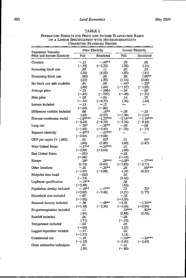
TABLE 2ESTIMATION RESULTS FOR PRICE AND INCOME ELASTICITIES BASED

ON A LINEAR SPECIFICATION WITH HETEROSCEDASTICITYCORRECTED STANDARD ERRORS

Dependent Variable: Price Elasticity Income ElasticityPrice and Income Elasticity Full Restricted Full Restricted

Constant

Increasing block rate

Decreasing block rate

No block rate info available

Average price

Shin price

Income included

Difference variable included

Discrete-continuous model

Long run

Segment elasticity

GDP per capita (X 1,000)

West United States

East United States

Europe

Other locations

Midpoint time trend

Loglinear specification

Population density included

Household size included

Seasonal dummy included

Evapotranspiration included

Rainfall included

Temperature included

Lagged dependent variable

Commercial use

Other estimation techniques

-.12(-.38)

.05(.34).003(.02).01(.09)

-.25(-.44)-.03

(-.34)-.12

(-.65).08(.65)

-1.07***

(-6.24)-. 26*

(-1.65)-. 67**

(-2.04).01

(.66)-. 17**

(-2.03)-.005

(-.06).28*

(1.73)-. 20

(-1.07)-. 005

(-.74)-. 15**

(-2.48)-. 18**

(-2.02)-.07

(-1.02)-.38

(-1.48).11(.84).06(.71)

-.04(-.63)-.17

(-1.37)-.19

(-1.13).01(.16)

-. 40** .20(-2.22) (.38)

.11 .02(1.05) (.03)

.06 .96(.55) (1.14).04 -. 44*(.64) (-1.87)

-.0004 -. 04(-.007) (-.46)-.06 .14

(-0.75) (.36)-.12 -

(-.86).18** -.59

(2.07) (-1.29)-1.25*** -1.14***

(-8.79) (-3.74)-. 28** -.06

(-2.43) (-.32)- .67*** -

(-2.60).02* .01

(1.89) (.40)-. 21*** .01

(-3.64) (.08)-.08

(-.42).29*** -1.08*

(3.02) (-1.83)-. 29** .24

(-2.00) (.74).03

(1.44).08

(.62)-. 17** .27

(-2.48) (1.21)-.33

(-1.39)-. 48** -1.23

(-2.36) (-1.60).74**

(2.88)-. 08

(-.33).03

(.23).02

(.14)-. 56*

(-2.40)-.21

(-.86)

.06(.21).24

(.81)1.09**

(2.00)-. 33*

(-1.85)-. 05

(-.51).20

(.44)

-.53(-1.21)-I 19***

(-5.10)-.08

(-.71)

.04*(1.87)

-. 77***(-2.71)

.60***(4.32)

.22*(1.77)

- 1.30**(-2.04)

.82**(2.55)

-. 30***(-2.69)

300 May 2003


TABLE 2 (CONTINUED)

Dependent Variable: Price Elasticity Income ElasticityPrice and Income Elasticity Full Restricted Full Restricted

Daily data -.08 -1.44** -. 93(-.64) (-2.40) (-4.09)

Monthly data -. 22** -. 22*** -. 95* -. 79(-2.08) (-2.66) (-1.79) (-3.22)

Household level data -.09 .16(-1.16) (.92)

Cross section data .04 .04(.33) (.13)

Panel data .30** .27*** .79*** .84***(2.51) (3.13) (3.12) (2.84)

Winter data .13** .10*** .24*(2.39) (2.65) (2.06)

Summer data -. 25** -. 28** .23 .30*(-2.24) (-2.37) (1.46) (1.97)

Unpublished studies .27* .28*** .59* .78***(1.93) (3.68) (1.86) (3.40)

R2-adj. .32 .33 .39 .42F test 5.03*** 7.61*** 4.14*** 6.74***Log Likelihood -140.12 -143.85 -130.87 -133.75Akaike Info. Crt. 1.18 1.13 2.04 1.92Log Amemiya Prob. Crt. -1.65 -1.71 -.80 -.91N 296 296 161 161

1. Following the discussion in Section 2,we include variables reflecting differ-ences in microeconomnic theory andeconometric methods. Specifically, weinclude variables relating to the type oftariff system (increasing and decreas-ing block rates, and a flat rate systemvs. those for which no information isavailable), the price variable (fixed, av-erage, marginal, or Shin), whether ornot the price elasticity is conditionedon income, and the modeling approach(inclusion of a difference variable, andapplication of the discrete-continuouschoice approach). GDP per capita isused to account for income differencesacross studies. Finally, short and longterm, and point and segment elasticitiesare distinguished.

2. Spatio-temporal dynamics are repre-sented by means of dummy variablesrelated to location (West United States,East United States, Europe and othercountries vs. the United States as theomitted category), and a linear time-

trend referring to the mid-point of thefirst and last year to which the data per-tain.

3. Estimation characteristics of the pri-mary studies are represented by meansof information about the functionalform (loglinear vs. other functionalforms), the conditioning variablesused in the underlying studies (pop-ulation density, household size, sea-sonal dummy, evapotranspiration, rain-fall, temperature, the lagged dependentvariable, and commercial use), and avariable indicating whether an estima-tor different from OLS is used.

4. The potential influence of the type ofdata is operationalized by means ofthe frequency of observation (dailyor monthly data vs. yearly data asthe omitted category), the aggregationlevel (individual or household data vs.aggregate data as the omitted cate-gory), and the type data series (crosssection or panel data vs. time seriesdata as the omitted category).

79(2) 301

Land Economics

5. Differences in terms of publication sta-tus are included by means of a dummyvariable for unpublished studies.

With respect to the functional form of themeta-regression, we believe that the use of aBox-Cox transformation accounting for non-linearities is not the appropriate solution. Themain reason for what looks like a non-linearpattern is the statistical principle that esti-mates based on fewer observations are lessefficient. Consequently, a Box-Cox transfor-mation is likely to provide a good fit, butno substantive explanatory power can beattached to it. It merely replicates a statisticalprinciple, and all estimates, regardless ofhow precise they are, are given the sameweight. The real problem is that meta-regres-sions are inherently heteroscedastic, becausethe effect sizes of different primary studiesare estimated with differing numbers of ob-servations. We therefore use a linear specifi-cation, and correct for heteroscedasticity byusing White-adjusted standard errors.8

The estimation results for both priceand income elasticities, with the variablesgrouped according to the above categories,are presented in Table 2. Since we do not usea Box-Cox transformation the price elastici-ties have been defined on the usual interval[--, 0]. Table 2 contains the results for the"Full Model" and for a "Restricted Model"in which conditioning variables from catego-ries 2-5 that are not significantly differentfrom zero are excluded using Theil's (1971)backward stepwise elimination strategy.

It is remarkable that elasticities underblock rate pricing are not significantly differ-ent from those under a flat rate system, ex-cept for income elasticities under decreasingblock rates in the restricted model. From theother microeconomic variables, it is only theinclusion of the difference variable on priceelasticities in the restricted model that is sig-nificantly different from zero. Most pro-nounced, however, is the effect of the two-error model. The effect of long vs. short runvalues conforms to expectations, althoughthe difference is only significant for price-elasticities. The income elasticity sampledoes not contain segment elasticities, but forthe price elasticity sample, they are signifi-

cantly higher. The effect of GDP per capitaacross studies is interesting: it is significantlypositive for price and income elasticities inthe restricted model, indicating that priceelasticities are generally smaller in absolutevalue (i.e., more inelastic) and income elas-ticities are higher in richer countries.

Table 2 also shows that elasticities tend tobe smaller in Europe as compared to theUnited States, and within the United States,price elasticities are greater in absolute valuein the arid West. The latter may be the resultof water use for purposes that are more elas-tic, such as irrigation (Espey, Espey, andShaw 1997). From the estimation character-istics, the climate-related variables have asystematic influence on the magnitude of theelasticities. Some of the data characteristicsare significantly different from zero as well.A final interesting result is that unpublishedstudies tend to report smaller absolute valuesof the price elasticity, and greater incomeelasticity values. The result with respect toprice elasticities contradicts the typical fea-ture of publication bias: "exaggerated" ef-fects, in this case high absolute values of theelasticities, have a lower probability of beingpublished (Card and Krueger 1995; Ashen-felter, Harmon, and Oosterbeek 1999).

The Impact of Differing Tariff Systems

We re-estimate the specification devel-oped in the preceding section on a subset ofthe sample for which information on the tariffstructure is available, in order to assess the im-pact of differing tariff systems more accu-rately. The results are reported in Table 3. Forprice elasticities, we again use the backwardstepwise elimination strategy. For incomeelasticities, this is not feasible because of thelimited number of observations for which wehave conclusive information about the ratestructure. With the number of observations be-

' The results of a Box-Cox specification do not alterthe main conclusions of our analysis. A comparison ofthe linear and the Box-Cox results is available from thewebsite mentioned in footnote 2. We present the linearresults in this article in order to avoid having to omitnegative income elasticities from the meta-sample, andbecause the interpretation of the coefficients of the lin-ear model is more straightforward.

302 May 2003


TABLE 3ESTIMATION RESULTS FOR PRICE AND INCOME ELASTICITIEs BASED ON A

LINEAR SPECIFICATION WITH HETEROSCEDASTICITY CORRECTED STANDARDERRORS FOR A SUBSAMPLE FOR WHICH INFORMATION ON THE TARIFF

STRUCTURE Is AVAILABLE

Dependent Variable: Price Elasticity Income ElasticityPrice and Income Elasticity Full Restricted Restricted

Constant 2.24*** .40 -. 97***(2.70) (1.60) (-2.87)

Increasing block rate -.16 -. 14* -. 41**(-1.60) (-1.77) (-2.50)

Decreasing block rate -.13 -.07 .61*(-1.11) (-.87) (1.89)

Average price -.23*** -. 19*** .48*(-3.40) (-3.42) (1.75)

Shin price -.11 -.13 2.98**(-1.28) (-1.55) (2.33)

Income included -1.17* -.03(-1.97) (-.18)

Difference variable included -.07 -.08 .93***(-.61) (-1.23) (3.22)

Discrete-continuous model -1.09*** -1.04*** .05(-4.99) (-12.39) (.21)

Longrun -.01 -.10 -.08(-.07) (-1.30) (-.53)

Segment elasticity -2.60*** - 1.28***(-3.58) (-3.32)

GDP per capita (X 1,000) -. 14*** -.04*** .06***(-3.13) (-3.82) (3.53)

West United States .75** .24*** -(2.59) (3.77)

East United States .21(1.34)

Europe -. 69***(-2.74)

Other locations -.38*(-1.82)

Midpoint time trend .05*** .009***(2.76) (2.83)

Loglinear specification .08(1.03)

Population density included .43(1.63)

Household size included -.33 -. 19*** -(-1.02) (-2.85)

Seasonal dummy included -.50*** -. 29*** -(-3.61) (-4.97)

Evapotranspiration included -.18(-1.43)

Rainfall included -.07(-.42)

Temperature included :03(.40)

Lagged dependent variable -. 06(-.34)

Commercial use .26(1.26)

Other estimation techniques -.12(-1.25)

Daily data .47

303

Land Economics

TABLE 3 (CONTINUED)


(1.47)Monthly data -1.27*** -.57*** -

(-3.30) (-4.14)Household level data -.09

(-.52)Cross section data -. 38***

(-2.64)Panel data 1.15** .58*** -

(2.61) (4.01)Winter data .16

(1.14)Summer data -.42*** -. 41*** -

(-3.29) (-6.78)Unpublished studies -. 10

C(-.60)

R2-adj. .23 .32 .43F test 2.10*** 4.33*** 7.28***Log Likelihood -52.10 -54.78 -78.35Akaike Info. Crt. 1.40 1.18 2.61LogAmemiya Prob. Crt. -1.42 -1.65 -. 23N 123 123 67

ing as low as 67, serious multi-collinearity in-flates standard efrror estimates, and we there-fore report a "base case" model in which onlythe microeconomic variables are included.

The results show that the effects of the mi-croeconomic variables are now much morepronounced. Increasing block rate pricingmakes the demand for water more elastic, butthe income elasticity tends to be lower. De-creasing block rate systems do not have asignificant effect on price elasticities, but theincome elasticities are significantly higher.The nexus of average and Shin prices in-creases the absolute value of the elasticitiesas compared to marginal prices, the latterin particular for income elasticities. Inclu-sion of a difference variable and the spec-ification of the demand for water as a dis-crete-continuous choice problem both havean effect, but the former only on income elas-ticities and the latter on price elasticities. Thesignificant difference between short and longrun elasticities disappears, but GDP per cap-ita is now significantly different from zerofor both price and income elasticities. Higherincome areas tend to have higher price andincome elasticities (in absolute terms).

Except for an occasional case, the signand significance of the control variables issimilar to those reported for the full sample.The spatial variables are an exception: thesign for the arid West of the United Statesis now positive, and the price elasticities forEurope are greater than in the United States.

The Impact of Differing MicroeconomicBehavioral Approaches

Some of the microeconomic variables al-ways appear in specific combinations, andcan be categorized as different microeco-nomic behavioral approaches to modelingresidential water demand. We distinguish thefollowing approaches.

1. The naive approach uses average orfixed prices, without conditioning onincome (except for income elasticities),and models demand as a continuouschoice.

2. The conditional approach conditionsfor income differentials, uses either av-erage or fixed prices, or marginal orShin prices, and models demand as acontinuous choice.

304 May 2003


TABLE 4(PARTIAL) ESTIMATION RESULTS FOR PRICE AND INCOME ELASTICITIES BASED

ON FOUR DIFFERENT BEHAVIORAL APPROACHES AND A LINEAR SPECIFICATIONWITH HETEROSCEDASTICITY CORRECTED STANDARD ERRORs,

FOR A SUBSAMPLE FOR WHICH INFORMATION ON THETARIFF STRUCTURE Is AVAILABLE


Constant 2.02** .16 -. 91**(2.42) (.63) (-2.37)

Increasing block rate -. 17* -. 26*** -. 36**(-1.77) (-3.65) (-2.09)

Decreasing block rate -.15 -.17** .57(-1.31) (-2.46) (1.62)

Conditional income approach with -1.16* .06 __baverage/fixed price (-1.93) (.31)

Conditional income approach with -. 99* .18 .79marginal/Shin price (-1.67) (.98) (1.20)

Corrected conditional income approach -. 99* .13 .41**(-1.69) (.64) (2.41)

Discrete-continuous choice approach -2.06*** -. 77*** .39(-3.30) (-3.99) (1.61)

Long run -.007 -.08 -.31(-.05) (-.96) (-.18)

Segment elasticity -2.57*** -1.48***(-3.47) (-3.55)

GDP per capita (X 1,000) -.14*** -. 04*** .09***(-3.15) (-3.26) (3.44)

R2-adj. .24 .31 .18F test 2.17*** 4.08*** 3.05***Log Likelihood -52.25 -54.61 -91.30Akaike Info. Crt. 1.39 1.20 2.96LogAmemiya Prob. Crt. -1.44 -1.64 .13N 123 123 67

The specifications for price elasticities also contain several control variables. Because the coeffi-cients are virtually identical to those presented in Table 3, they are not reported here.

I For income elasticities the conditional income approach with average/fixed price is identical tothe naive approach, which is the omitted category.

3. The sophisticated conditional ap-proach conditions for income differ-entials, uses marginal or Shin prices,includes a difference variable, andmodels demand as a continuous choice.

4. The discrete-continuous choice ap-proach conditions for income differen-tials, uses marginal prices, includes adifference variable, and models de-mand as a discrete-continuous choice.

For income elasticities, the naive ap-proach and the conditional income approach

with average or fixed prices coincide, be-cause income elasticities are by defini-tion conditioned on income. As the speci-fication of the above approaches is merely aregrouping of dummy variables used ear-lier, the estimation results are very similarfor all variables except for the behavioralmodel variables. The results are presented inTable 4.

The results for block rate pricing, GDPper capita, and long vs. short run and seg-ment vs. point elasticities conform to thosereported in Table 3, with the results for block

79(2) 305

Land Economics

rate pricing being slightly more significant.Table 4 shows that the more sophisticatedbehavioral approaches, such as the (sophisti-cated) conditional approaches and the dis-crete-continuous approach, increase the ab-solute value of both price and incomeelasticities. This is not the case for the re-stricted model referring to price elasticities,and for the conditional income approach withmarginal or Shin prices in the case of incomeelasticities. Subsequent F-tests on the restric-tion that the estimated coefficients of the dif-ferent approaches are the same (in the so-called restricted models), is rejected for priceelasticities (F = 6.97, p = .00), but notrejected for income elasticities (F = .57,p = .64). In the case of price elasticitiesF-tests on the behavioral approaches havingthe same effect are accepted for all pair-wise comparisons, except for those with thediscrete-continuous approach (all p-levels <.10). In sum, the discrete-continuous ap-proach constitutes a noticeably different be-havioral modeling approach resulting insubstantially greater price elasticities, but in-come elasticities based on this approach can-not be discerned from those based on othermodeling approaches.

V. CONCLUSION

In reviewing the literature on water de-mand modeling, Hewitt and Hanemann(1995) provide a "history" of residentialwater demand modeling, and they point outthat studies differ along many dimensions.The meta-analysis reported in this articlegives a systematic statistical account of thesedifferences, in a multivariate framework. Theanalysis goes beyond the Espey, Espey, andShaw (1997) analysis, because the currentanalysis is concerned with a larger sample ofstudies, includes income elasticities, containsthree studies using the discrete-continuousapproach, and accounts for differences in in-come levels across studies through GDP percapita levels.

We have taken special care to assess theimpact of differing microeconomic charac-teristics of the primary studies. In sum, wefind that residential water demand is rela-tively price-elastic, but income elasticities

are relatively inelastic, under increasingblock rate pricing. In studies using sophisti-cated modeling approaches (such as marginalor Shin prices, income differential controls,a difference variable, and a discrete-continu-ous choice setup), price and income elastici-ties are relatively high. There is, however animportant proviso: the use of the discrete-continuous model does not have a signifi-cant impact on income elasticities. Phrasedin terms of the four behavioral models dis-tinguished above, the discrete-continuousmodel is characterized by significantlyhigher price elasticities of demand, whereasfor income elasticities no significant differ-ences between the four approaches can bediscerned. Segment price elasticities are sub-stantially greater, and there is some (althoughnot very robust) evidence that long run elas-ticities are larger in magnitude. Finally, it iscrucial to account for income differencesamong studies. We include GDP per capitaas a proxy, and find that the absolute magni-tude of price and income elasticities is sig-nificantly greater for areas with higher in-comes.

Although the attention for water scarcityissues would lead one to expect that elastici-ties have increased over time, this is not thecase: there is no significant time trend in theelasticity values. The geographical dimen-sions of variation are less clear. In the UnitedStates, elasticity values are rather homoge-neous, except for the arid West. The elastici-ties in Europe and in other locations are dis-tinctly different from those in the UnitedStates. For both Europe and the West UnitedStates, the results are however not robustacross different meta-samples. It is thereforestill unclear where (absolute) elasticity val-ues are highest.

The qualitative analysis of Hewitt and Ha-nemann (1995) and the meta-analysis of Es-pey, Espey, and Shaw (1997) as well as thecurrent meta-analysis show that functionalspecification, aggregation level, data charac-teristics, and estimation issues are associatedwith different elasticity values. The directionand significance of these effects is, however,not yet robust. This clearly shows that addi-tional primary research is needed. Future pri-mary research is also called for to settle the

306 May 2003


issue of the appropriateness of the discrete-continuous choice approach to modeling resi-dential water demand.

References

Agthe, D. E., and R. B. Billings. 1980. "DynamicModels of Residential Water Demand." WaterResources Research 16 (3): 476-80.

Ashenfelter, O., C. Harmon, and H. Oosterbeek.1999. "A Review of Estimates of theSchooling/Earnings Relationship, with Testsfor Publication Bias." Labour Economics 6(4): 453-70.

Baumann, D. D., J. J. Boland, and W. M. Hanem-ann. 1998. Urban WaterDemand Managementand Planning. New York: McGraw-Hill.

Billings, R. B. 1990. "Demand-Based Benefit-Cost Model of Participation in Water Project."Journal of Water Resource Planning andManagement 116 (5): 593-609.

Card, D., and A. B. Krueger. 1995. "Time-SeriesMinimum-Wage Studies: A Meta-Analysis."American Economic Reviewv 85 (2): 238-43.

Cooper, H., and L. V. Hedges, eds. 1994. TheHandbook of Research Synthesis. New York:Sage Publishers.

Dalhuisen, J. M., R. J. G. M. Florax, H. L. F. deGroot, and P. Nijkamp. 2001. "Price and In-come Elasticities of Residential Water De-mand: Why Empirical Estimates Differ."Tinbergen Institute Discussion Paper, No.01-057/3. Tinbergen Institute, Amsterdam-Rotterdam.

Danielson, L. E. 1979. "An Analysis of Residen-tial Demand for Water Using Micro Time Se-ries Data." Water Resouirces Research 15 (4):763-67.

Espey, M., J. Espey, and W. D. Shaw. 1997."Price Elasticity of Residential Demand forWater: A Meta-Analysis." Water ResourcesResearch 33 (6): 1369-74.

Glass, G. V. 1976. "Primary, Secondary, andMeta-Analysis of Research." Educational Re-search 5:3-8.

Greene, W. H. 2000. Econometric Analysis. Up-per Saddle River, N.J.: Prentice Hall.

Hausman, J. A. 1985. "The Econometrics ofNonlinear Budget Sets." Econometrica 53 (6):1255-82.

Hedges, L. V., and I. Olkin. 1985. StatisticalMethods for Meta-Analysis. New York: Aca-demic Press.

Hewitt, J. A. 1993. "Watering Households: TheTwo-Error Discrete-Continuous Choice Model

of Residential Water Demand." Ph.D. diss.,University of California, Berkeley.

Hewitt, J. A., and W. M. Hanemann. 1995. "ADiscrete/Continuous Choice Approach to Res-idential Water Demand under Block Rate Pric-ing." Land Economics 71 (May): 173-92.

Hogarty, T. F., and R. J. Mackay. 1975. "The Im-pact of Large Temporary Rate Changes onResidential Water Use." Water Resources Re-search 11 (6): 791-94.

Howe, C. W., and F. P. Linaweaver. 1967. "TheImpact of Price on Residential Water Demandand its Relation to System Design and PriceStructure." Water Resources Research 3 (1):13-32.

Lyman, R. A. 1992. "Peak and Off-Peak Resi-dential Water Demand." Water Resources Re-search 28 (9): 2159-67.

Martin, R. C., and R. P. Wilder. 1992. "Residen-tial Demand for Water and the Pricing ofMunicipal Water Services." Public FinanceQOtarterly 20 (1): 93-102.

Moffitt, R. 1986. "The Econometrics of Piecewise-Linear Budget Constraints." Journal of Busi-ness and Economics Statistics 4 (3): 317-28.

Nieswiadomy, M. L. 1992. "Estimating UrbanResidential Water Demand: Effects of PriceStructure, Conservation, and Education." Wa-ter Resources Research 28 (3): 609-15.

Nieswiadomy, M. L., and D. J. Molina. 1989."Comparing Residential Water Demand Esti-mates under Decreasing and Increasing BlockRates Using Household Data." Land Econom-ics 65 (Aug.): 280-89.

Nordin, J. A. 1976. "A Proposed Modification ofTaylor's Demand Analysis: Comment." TheBell Journal of Economics 7 (2): 719-21.

OECD. 1998. Pricing of Water Services in OECDCountries: Update. Paris: OECD.

. 1999. The Price of Water: Trends inOECD Countries. Paris: OECD.

Opaluch, J. J. 1982. "Urban Residential Demandfor Water in the United States: Further Discus-sion." Land Economics 58 (May): 225-27.

.1984. "A Test of Consumer Demand Re-sponse to Water Prices: Reply." Land Eco-noinics 60 (Nov.): 417-21.

Rietveld, P., J. Rouwendal, and B. Zwart. 1997."Equity and Efficiency in Block Rate Pricing:Estimating Water Demand in Indonesia."Tinbergen Institute Discussion Paper, No.97-072/3. Tinbergen Institute, Amsterdam-Rotterdam.

Shin, J.-S. 1985. "Perception of Price when In-formation Is Costly: Evidence from Residen-tial Electricity Demand." Review of Econom-ics and Statistics 67 (4): 591-98.

307

Land Economics

Stanley, T. D. 2001. "Wheat from Chaff: Meta-Analysis as Quantitative Literature Review."Journal of Economic Perspectives 15:131-50.

Taylor, L. D. 1975. "The Demand for Electricity:A Survey." The Bell Journal of Economics 6(1): 74-110.

Theil, H. 1971. Principles of Econometrics. NewYork: Wiley.

Van den Bergh, J. C. J. M., K. J. Button, P.Nijkamp, and G. C. Pepping. 1997. Meta-Analysis in Environmental Economics. Dor-drecht: Kluwer Academic Publishers.

White, H. D. 1994. "Scientific Communicationand Literature Retrieval." In The Handbook ofResearch Synthesis, ed. H. Cooper and L. V.Hedges. New York: Sage Publishers.

308 May 2003

COPYRIGHT INFORMATION

TITLE: Price and Income Elasticities of Residential WaterDemand: A Meta-Analysis

SOURCE: Land Econ 79 no2 My 2002WN: 0230601962010

The magazine publisher is the copyright holder of this article and itis reproduced with permission. Further reproduction of this article inviolation of the copyright is prohibited. To contact the publisher:http://www.wisc.edu/wisconsinpress/

Copyright 1982-2003 The H.W. Wilson Company. All rights reserved.

price and income elasticities of residential water...

Documents