a meta-analysis of hedonic studies to assess the property
TRANSCRIPT

Resources 2014, 3, 31-61; doi:10.3390/resources3010031
resources ISSN 2079-9276
www.mdpi.com/journal/resources
Article
A Meta-Analysis of Hedonic Studies to Assess the Property
Value Effects of Low Impact Development
Marisa J. Mazzotta 1,*, Elena Besedin
2 and Ann E. Speers
2
1 Atlantic Ecology Division, U.S. EPA Office of Research and Development, 27 Tarzwell Drive,
Narragansett, RI 02882, USA 2
Abt Associates Inc., 55 Wheeler Street, Cambridge, MA 02138, USA;
E-Mails: [email protected] (E.B.); [email protected] (A.E.S.)
* Author to whom correspondence should be addressed; E-Mail: [email protected];
Tel.: +1-401-782-3026; Fax: +1-401-782-3030.
Received: 28 October 2013; in revised form: 24 December 2013 / Accepted: 7 January 2014 /
Published: 21 January 2014
Abstract: Stormwater runoff from urban areas is a significant source of water pollution in
the United States. Many states are promoting low impact development (LID) practices,
which provide a variety of direct and ancillary ecosystem services. We describe a
meta-analysis designed to evaluate the property value benefits of LID practices that reduce
impervious surfaces and increase vegetated areas in developments, and present an example
application to a hypothetical land use scenario. From the many hedonic property valuation
studies of the benefits of general open space, we identified 35 studies that valued open
spaces that were similar in nature to the small, dispersed open spaces characteristic of LID.
The meta-regression estimates the percent change in a home’s value for an observed
percent change in open space within a specific radius of a parcel, based on changes
expected to result from LID approaches that increase green spaces. Our results indicate that
the design and characteristics of a project affect the magnitude of benefits, and that values
decline with distance. More broadly, the meta-analysis shows percent change and
proximity are robust determinants of household willingness to pay for aesthetic and other
services associated with local availability of small, dispersed open spaces resulting from
LID, but that values for other features, including type of vegetation and recreational use
may be site-specific. Policymakers and developers could draw on our synthesis of site
characteristics’ effects to maximize benefits from open space associated with LID.
OPEN ACCESS
Resources 2014, 3 32
Keywords: meta-analysis; property values; hedonic valuation; low impact development;
environmental site design; green infrastructure; ecosystem services; benefit transfer;
stormwater; open space
1. Introduction
Stormwater runoff from urban areas is a significant source of pollution to our nation’s waters.
According to the National Research Council report Urban Stormwater Management in the United
States, stormwater discharges from the built environment remain one of the greatest challenges of
modern water pollution controls, “as this source of contamination is a principal contributor to water
quality impairment of waterbodies nationwide [1] (page vii)” Many states are using regulations,
incentives, or educational campaigns to encourage use of low impact development (LID) or green
infrastructure (GI) practices that harvest, infiltrate, and promote evapotranspiration to prevent
stormwater runoff. Successful LID and GI practices provide ecosystem services by increasing the
amount of stormwater retained on site, thereby improving surface water quality and hydrology in water
bodies that receive stormwater runoff, enhancing groundwater recharge, reducing flood risk and
preventing soil erosion [2].
Along with these primary benefits, many LID and GI practices can provide additional ecosystem
services such as carbon sequestration, air quality improvements, microclimate regulation, wildlife
habitat, water purification, and aesthetic benefits of augmented landscape features. The improved
ecosystem services, in particular augmented landscape features, may be reflected in increased property
values for both newly developed properties in locations employing these techniques, and existing
properties located near areas with increased green spaces.
Comprehensive analysis of the benefits and costs of LID and GI should include values of direct and
ancillary ecosystem services provided by these practices. In this paper, we present a meta-analysis
designed to evaluate the property value effects from the increased green spaces in areas developed
using LID and GI practices, as compared to those provided by conventional development. The green
spaces resulting from LID and GI practices are typically small and dispersed in nature, and often do
not provide recreational values [3–6]. Thus, our investigation focuses on values for small, dispersed
green spaces, and also evaluates the differences in value between open spaces with and without
recreational uses. Such values have not been investigated in a meta-analysis to date, although there is
growing policy emphasis on promoting LID and GI practices. We present an example application of
the meta-regression to a hypothetical land development scenario.
LID encompasses a wide variety of development approaches that often attempt to integrate “site
design, natural hydrology, and smaller controls to capture and treat runoff” [2]. Applications range from
subtle to dramatic site alterations, some of which increase the percent of vegetated and tree-covered land
in a subdivision relative to conventional subdivisions. Examples of LID implementation include,
“…preserving natural areas, minimizing and disconnecting impervious cover, minimizing land
disturbance, conservation (or cluster) design, using vegetated channels and areas to treat stormwater,
and incorporating transit, shared parking, and bicycle facilities to allow lower parking ratios” [7].
Resources 2014, 3 33
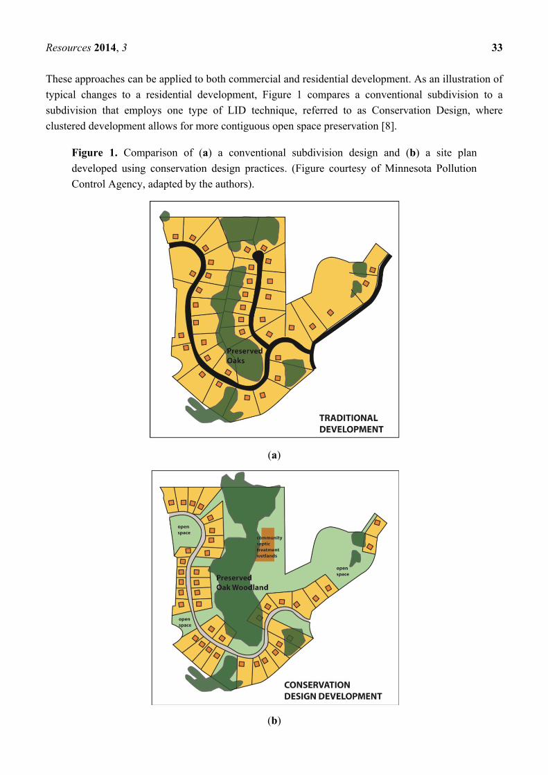
These approaches can be applied to both commercial and residential development. As an illustration of
typical changes to a residential development, Figure 1 compares a conventional subdivision to a
subdivision that employs one type of LID technique, referred to as Conservation Design, where
clustered development allows for more contiguous open space preservation [8].
Figure 1. Comparison of (a) a conventional subdivision design and (b) a site plan
developed using conservation design practices. (Figure courtesy of Minnesota Pollution
Control Agency, adapted by the authors).
(a)
(b)
Resources 2014, 3 34
Although residential LID sometimes results in smaller lot sizes and less space between homes, it
can also provide more open space, and better views of that open space, than conventional subdivision
design. In some cases recreational opportunities may also be enhanced (e.g., by including soccer fields
or walking trails). To the extent buyers and sellers in the housing market are aware of and perceive
amenity benefits from LID, we expect that such benefits will be capitalized into the value of a home.
While homes both within (on-site) and near (off-site) an LID development experience additional green
space, on-site parcel values may reflect the net effect of increased green space and changes in other
project attributes, such as reduced parking area, the qualitative feel of living in a clustered
neighborhood, etc. As such, there may be qualitative differences in observed property value effects for
on-site vs. off-site but nearby properties.
Existing studies show mixed and location-specific relationships between property value effects of
on-site lot size and shared open space. Some studies have demonstrated that, while in general buyers
prefer larger lot size, they are willing to trade a decrease in lot size for larger shared open space or for
decreased distance to shared open space [9–12]. Typically, this trade does not occur at a one-to-one
rate of substitution; further, the rates of substitution have been shown to vary by location [10,11]. In
some cases, larger lots are more valuable than increased shared open space, while in other cases shared
open space compensates for smaller lot sizes [10,11].
Open space effects on nearby (off-site) property values are also well studied. A large body of
economic literature provides insights into changes in property values due to changes in tree cover,
proximity to open space, or presence of parks or forested land in the neighborhood. Numerous studies
have shown that increased vegetated open space leads to increases in nearby residential property
values e.g., [9,13–18], although negative or inconclusive effects have also been reported [19–21].
However, very few studies directly address values related specifically to LID practices [5,9,12,16–18,22–27],
and many of these studies use non-uniform measures of open space to evaluate effects of these
practices on property values, rendering a direction comparison of the results infeasible.
However, conducting original hedonic pricing studies such as these to support analysis of land
management decisions is rarely feasible due to time or resource constraints. Thus, the majority of such
analyses rely on benefit transfer from existing economic literature. Previous benefit transfers that estimate
the effects of LID practices on property values have used point transfers of open space values [28,29]. If
the study site does not provide a very close match to the policy site, point value transfer is likely to
yield biased estimates. While functional transfers based on meta-analysis are not necessarily free of
such bias, they allow analysts to incorporate site specific factors (e.g., open space size and
characteristics) in the valuation function and thus reduce potential bias [30,31]. Meta-analysis is
increasingly being used to conduct and inform function-based benefit transfer [32–34] because it can
incorporate and address systematic variations in value [35–39]. While both the choice of a single study
for point transfer and the choice of multiple studies to include in a meta-analysis require the analyst to
make subjective judgments, meta-analysis allows analysts to synthesize information from a broad
range of locations, study site characteristics and open space attributes, thereby potentially offering
more robust estimates and minimizing transfer errors relative to point transfer [40].
An important factor in any benefit transfer is the ability of the study site or estimated valuation
equation to approximate the resource and context under which benefit estimates are desired. The open
space typical of LID developments will often be small and dispersed, rather than large and contiguous.
Resources 2014, 3 35
Furthermore, although LID open space does not generally provide recreational benefits, some developers
have begun purposively incorporating parks, sports fields, and other recreational features [5,41]. As is
common, data in our meta-analysis provide a close but not perfect match to the LID context. From the
many hedonic property valuation studies of the benefits of general open space, we identified 35 studies
that value open spaces similar in nature to the small, dispersed open space characteristic of many LID
practices. We estimate a meta-regression model (MRM) of the percent change in a home’s value for a
given percent change in open space area within a specified radius of the parcel. Additionally, because
our model is intended to be used for benefit transfer, following Boyle et al. [30], we examine various
factors that indicate whether the estimates are robust or fragile.
In Section 2, we discuss the selection of relevant studies, and characteristics and preparation of the data;
in Section 3 we discuss model specification and results; in Section 4 we present an example application;
and Section 5 is a summary of findings and implications for policy and management decisions.
2. Study Selection and Data Preparation
Study selection involves screening studies to ensure that they are appropriate to the goal of the
analysis and that they measure a consistent and theoretically appropriate effect [30]. Our study
objective is to predict the willingness to pay (WTP) for marginal changes in open space resulting from
policies that encourage or require LID practices relative to more conventional development
approaches. Through our process of study selection, we thoroughly screened studies and, through a
number of iterations and internal reviews of the data, eliminated many studies deemed irrelevant.
Following guidance from economic literature [30] we maintained theoretically consistent welfare
measures by including only values from hedonic studies to, and converted measures of open space
effects to a common metric—the percent open space within a given radius of a home.
To identify potentially relevant studies for the open space meta-analysis, we conducted an in-depth
search of the economic literature using a variety of sources and search methods. We reviewed over
180 studies, including nine stated preference studies, and over 100 hedonic studies of property value
changes from improved amenities associated with, or similar to those achieved from LID practices.
The remaining studies are either reviews of other studies; benefit transfers; general information on LID
practices, costs, and benefits; studies based on avoided costs; studies of public perceptions that do not
include values; or case studies of actual LID developments, most of which focus on costs to
developers. After further screening, we included data from 35 hedonic studies in the meta-analysis,
based on the following criteria:
Valuation method and values estimated: Selected studies were limited to those that used
hedonic valuation techniques to measure a percent change in home value. We excluded stated
preference studies to avoid issues related to different formulations of the dependent variable
and different welfare measures provided by hedonic and stated preferences studies.
Specific amenity valued: We eliminated studies that valued open spaces labeled as golf courses,
large parks or forests, water features, or agricultural land. We also excluded studies related to
any open space larger than 100 acres. Open spaces with these features are not generally
relevant to open spaces provided by LID practices.
Study location: Selected studies were limited to those conducted in the United States.
Resources 2014, 3 36
Ability to convert values to similar terms: Original studies estimated the value of open space
amenities in terms of a change in one of several different metrics: either a home’s distance to
open space, a home’s adjacency to open space, or the proportion of a home’s neighborhood
kept in open space. To complete a meta-analysis based on studies using different methods, we
first converted all measures into a single common metric—the proportion of a home’s
neighborhood in open space (measured by a specific radius around the home). Studies that
could not be converted because of a lack of information were not included in the final data set.
The 35 studies provided 119 observations, with multiple estimates of changes in property values
available from 26 studies. For each observation, we computed a measure of WTP for open space,
standardizing all reported results into an estimated percent change in property value given an observed
percentage change in open space, e.g., [42].
2.1. Converting Open Space Measures to Comparable Metrics
All of the original studies in our data set estimated property value premiums associated with open
space; however, individual studies used one of several measures of open space availability, including
percent of open space in a buffer surrounding a home, adjacency to open space and distance to open
space. To examine these studies in aggregate (i.e., in meta-analysis), we first converted all open space
measures into a common metric across studies: the percentage of land surrounding a home that is in
open space cover. Seventy of the 119 observations included in the model were originally in terms of
percent or area of open space feature(s) within a buffer area around homes; these observations were
used in their original form. In these studies, the size of the buffer areas ranged from 715 m2 to 8.14 km
2
(mean 1.02 km2), and the baseline percent open space within the buffers ranged from 0.24% to 99%
(mean 3.77%). Two observations were originally in terms of adjacency to open space, and 47 were
originally in terms of distance to open space. To convert measures of open space into a single metric
(the percentage of open space in a buffer surrounding a home) for these 49 observations, we applied
conversion methods developed by Kroeger [43] (see also [44]). We refer readers to Appendix 1 for
additional details on conversion methods.
2.2. Description of the Meta-Analysis Data
Studies used in the meta-analysis were conducted between 1996 and 2012, and applied standard,
generally accepted hedonic valuation methods. The 35 studies include 32 journal articles and
three academic or staff papers. All selected studies focus on the relationship between existing open
space and property values in the United States. None of the included studies examined exogenous
changes in open space (i.e., property values before and after a change in the actual amount of open
space on the ground); rather, studies examined variation in sales price based on variation in proximity
to, adjacency to, or the surrounding amount of open space. Beyond this, the studies vary in several
additional respects. Differences include the specific type, size and features of open space valued, size
of the surrounding area considered or distance to open space, population density of the study area, and
geographic region. Twenty-two of the observations value amenities on individual parcels, as opposed
to properties adjacent to or in proximity to open space.
Resources 2014, 3 37
We included studies evaluating a variety of open space types, and categorized these into four groups:
a general/combined category of vegetated open space, which includes all studies that either
estimate values for more than one type of open space as a group, simply specify “open space”
as the variable of interest, or that examine vegetated open space that is not primarily tree-covered;
a category for open space that is primarily tree-covered;
a category for riparian buffers and habitat; and
a category for wetlands.
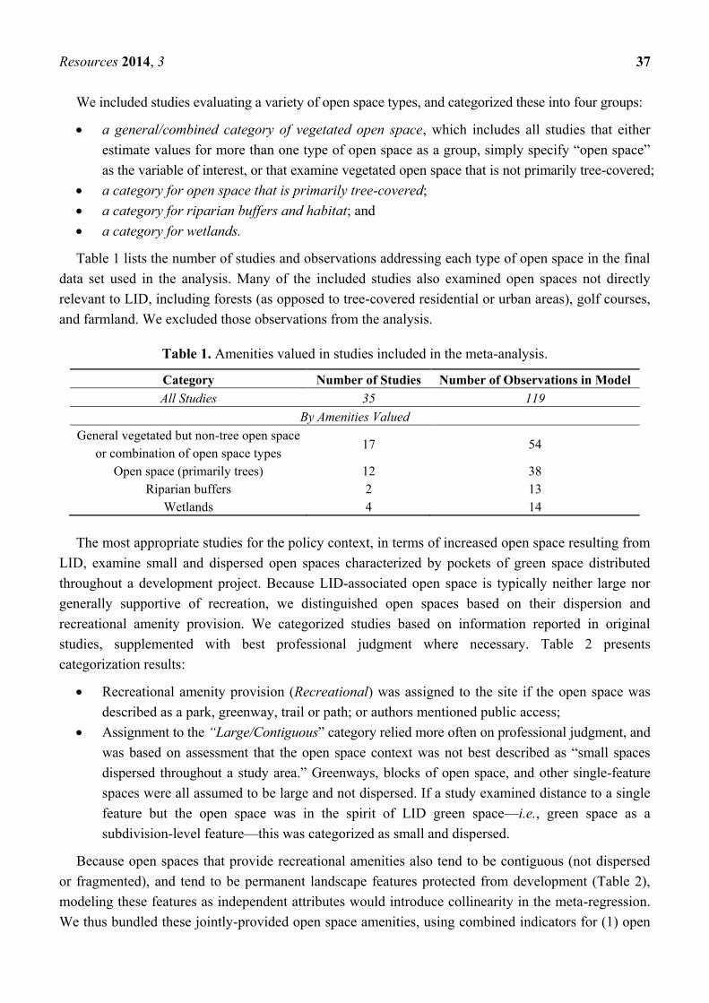
Table 1 lists the number of studies and observations addressing each type of open space in the final
data set used in the analysis. Many of the included studies also examined open spaces not directly
relevant to LID, including forests (as opposed to tree-covered residential or urban areas), golf courses,
and farmland. We excluded those observations from the analysis.
Table 1. Amenities valued in studies included in the meta-analysis.
Category Number of Studies Number of Observations in Model
All Studies 35 119
By Amenities Valued
General vegetated but non-tree open space
or combination of open space types 17 54
Open space (primarily trees) 12 38
Riparian buffers 2 13
Wetlands 4 14
The most appropriate studies for the policy context, in terms of increased open space resulting from
LID, examine small and dispersed open spaces characterized by pockets of green space distributed
throughout a development project. Because LID-associated open space is typically neither large nor
generally supportive of recreation, we distinguished open spaces based on their dispersion and
recreational amenity provision. We categorized studies based on information reported in original
studies, supplemented with best professional judgment where necessary. Table 2 presents
categorization results:
Recreational amenity provision (Recreational) was assigned to the site if the open space was
described as a park, greenway, trail or path; or authors mentioned public access;
Assignment to the “Large/Contiguous” category relied more often on professional judgment, and
was based on assessment that the open space context was not best described as “small spaces
dispersed throughout a study area.” Greenways, blocks of open space, and other single-feature
spaces were all assumed to be large and not dispersed. If a study examined distance to a single
feature but the open space was in the spirit of LID green space—i.e., green space as a
subdivision-level feature—this was categorized as small and dispersed.
Because open spaces that provide recreational amenities also tend to be contiguous (not dispersed
or fragmented), and tend to be permanent landscape features protected from development (Table 2),
modeling these features as independent attributes would introduce collinearity in the meta-regression.
We thus bundled these jointly-provided open space amenities, using combined indicators for (1) open
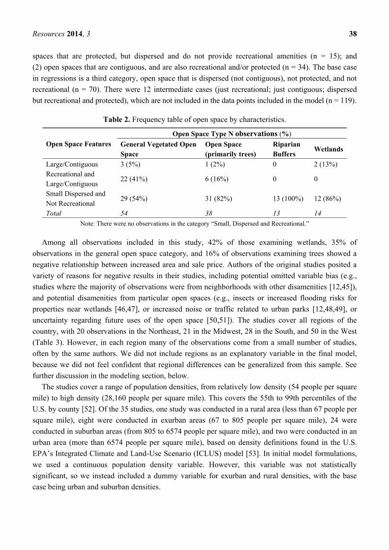
Resources 2014, 3 38
spaces that are protected, but dispersed and do not provide recreational amenities (n = 15); and
(2) open spaces that are contiguous, and are also recreational and/or protected (n = 34). The base case
in regressions is a third category, open space that is dispersed (not contiguous), not protected, and not
recreational (n = 70). There were 12 intermediate cases (just recreational; just contiguous; dispersed
but recreational and protected), which are not included in the data points included in the model (n = 119).
Table 2. Frequency table of open space by characteristics.
Open Space Features
Open Space Type N observations (%)
General Vegetated Open
Space
Open Space
(primarily trees)
Riparian
Buffers Wetlands
Large/Contiguous 3 (5%) 1 (2%) 0 2 (13%)
Recreational and
Large/Contiguous 22 (41%) 6 (16%) 0 0
Small Dispersed and
Not Recreational 29 (54%) 31 (82%) 13 (100%) 12 (86%)
Total 54 38 13 14
Note: There were no observations in the category “Small, Dispersed and Recreational.”
Among all observations included in this study, 42% of those examining wetlands, 35% of
observations in the general open space category, and 16% of observations examining trees showed a
negative relationship between increased area and sale price. Authors of the original studies posited a
variety of reasons for negative results in their studies, including potential omitted variable bias (e.g.,
studies where the majority of observations were from neighborhoods with other disamenities [12,45]),
and potential disamenities from particular open spaces (e.g., insects or increased flooding risks for
properties near wetlands [46,47], or increased noise or traffic related to urban parks [12,48,49], or
uncertainty regarding future uses of the open space [50,51]). The studies cover all regions of the
country, with 20 observations in the Northeast, 21 in the Midwest, 28 in the South, and 50 in the West
(Table 3). However, in each region many of the observations come from a small number of studies,
often by the same authors. We did not include regions as an explanatory variable in the final model,
because we did not feel confident that regional differences can be generalized from this sample. See
further discussion in the modeling section, below.
The studies cover a range of population densities, from relatively low density (54 people per square
mile) to high density (28,160 people per square mile). This covers the 55th to 99th percentiles of the
U.S. by county [52]. Of the 35 studies, one study was conducted in a rural area (less than 67 people per
square mile), eight were conducted in exurban areas (67 to 805 people per square mile), 24 were
conducted in suburban areas (from 805 to 6574 people per square mile), and two were conducted in an
urban area (more than 6574 people per square mile), based on density definitions found in the U.S.
EPA’s Integrated Climate and Land-Use Scenario (ICLUS) model [53]. In initial model formulations,
we used a continuous population density variable. However, this variable was not statistically
significant, so we instead included a dummy variable for exurban and rural densities, with the base
case being urban and suburban densities.

Resources 2014, 3 39
Table 3. Selected summary information for studies.
Author(s) and Year State N observations Radius, or range of
radii (m) Open Space Types
Abbott and Klaiber [54] AZ 3 305–610 General Vegetation
Acharya and Bennett [55] CT 2 402–1609 General Vegetation
Anderson and West [56] MN 1 469 General Vegetation
Bark et al. [48] AZ 12 210–1179 Riparian; General Vegetation
Bin [57] OR 2 1524–1676 Wetland
Bin and Polasky [47] NC 3 234–402 Wetland
Bolitzer and Netusil [58],
Lutzenhiser and Netusil [59]* OR 8 276–457 Trees; General Vegetation
Bowman et al. [17] IA 2 287–287 General Vegetation
Cho et al. [60] TN 2 2762–2925 General Vegetation
Cho et al. [61] TN 3 326–481 Trees
Cho et al. [10] TN 1 2422 General Vegetation
Cho et al. [62] TN 1 1609 Trees
Donovan and Butry [63] OR 1 30 Trees
Doss and Taff [46] MN 4 251–502 Wetland
Geoghegan et al. [64] MD 2 100–1000 General Vegetation
Hardie et al. [65] MD 1 235 Trees
Heintzelman [19] MA 6 161–1609 General Vegetation
Irwin [66] MD 2 400–400 General Vegetation
Kaufman and Cloutier [67] WI 1 368 General Vegetation
Kopits et al. [9] MD 1 415 General Vegetation
Mahan et al. [68] OR 3 1091–1091 Wetland
Munroe [45] NC 2 1070–1070 General Vegetation
Netusil [20]; Netusil et al. [69]* OR 14 17–805 Riparian; Wetland; Trees
Ready and Abdalla [50] PA 12 400–400 Trees; General Vegetation
Sander and Polasky [70] MN 3 226–612 Trees; General Vegetation
Sander et al. [71] MN 6 21–443 Trees; General Vegetation
Saphores and Li [72] CA 3 15–200 Trees
Shultz and King [73] AZ 1 5391 Riparian
Smith et al. [51] NC 4 61–114 General Vegetation
Stetler et al. [74] MT 3 250–250 Trees
Thorsnes [75] MI 2 229–486 Trees
Towe [76] MD 1 409 General Vegetation
Troy and Grove [77] MD 3 482–482 General Vegetation
White and Leefers [78] MI 2 805–805 General Vegetation
Williams and Wise [12] FL 2 157–1459 General Vegetation
Note: *: Studies were considered to be a single study in the model due to similarities in data, the same study
location, and common author.
Resources 2014, 3 40
3. Meta-Analysis Regression Model and Results
3.1. Variable Selection and Specification
Based on findings of the studies in the data set and the large hedonic literature, our initial
hypothesized model included a set of explanatory variables. We tested variables accounting for
systematic variation in open space types and amenities, original study site housing markets, and
interactions between sale price and proximity to open space. Incorporating these variables allows one
to use the meta-analysis to tailor function-based benefits transfer between study and policy sites. Not
all variables were ultimately included in the MRM due to data limitations (see below). We initially
tested models including the following variables:
type of open space;
percent change in open space;
size of the radius indicating maximum distance from open space amenity, both as continuous
and categorical variables;
size of open space amenity;
population density of the study region;
income (proxied by mean or median home value in the original studies);
lot size;
geographic region;
whether the open space occurs on a property; or off-site, but near a property;
whether the open space is protected;
whether the open space provides recreational amenities;
whether the open spaces considered are dispersed/fragmented.
One would expect variations in value of open space across regions, particularly in arid versus wet
regions, and in more urbanized versus less urbanized regions (although this difference may be captured
by the population density variable). However, regional variable coefficients were not statistically
significant. Addition of the regional dummies did not improve the fit of the model or the magnitude or
significance of other variables. Moreover, studies for particular open space types were often conducted
by the same authors in the same geographic areas, which may result in “authors’ effects” rather than
geographic effects. Thus, we excluded geographic region in the final MRM. We also tested for
significant differences in value for studies converted from distance or adjacency measures (as
described above), by including dummy variables for those studies in preliminary models, and found no
significant differences. Although the lot size variable is not significant, we elected to include it in the
final MRM because of the potential tradeoffs between lot size and open space. Results for this variable
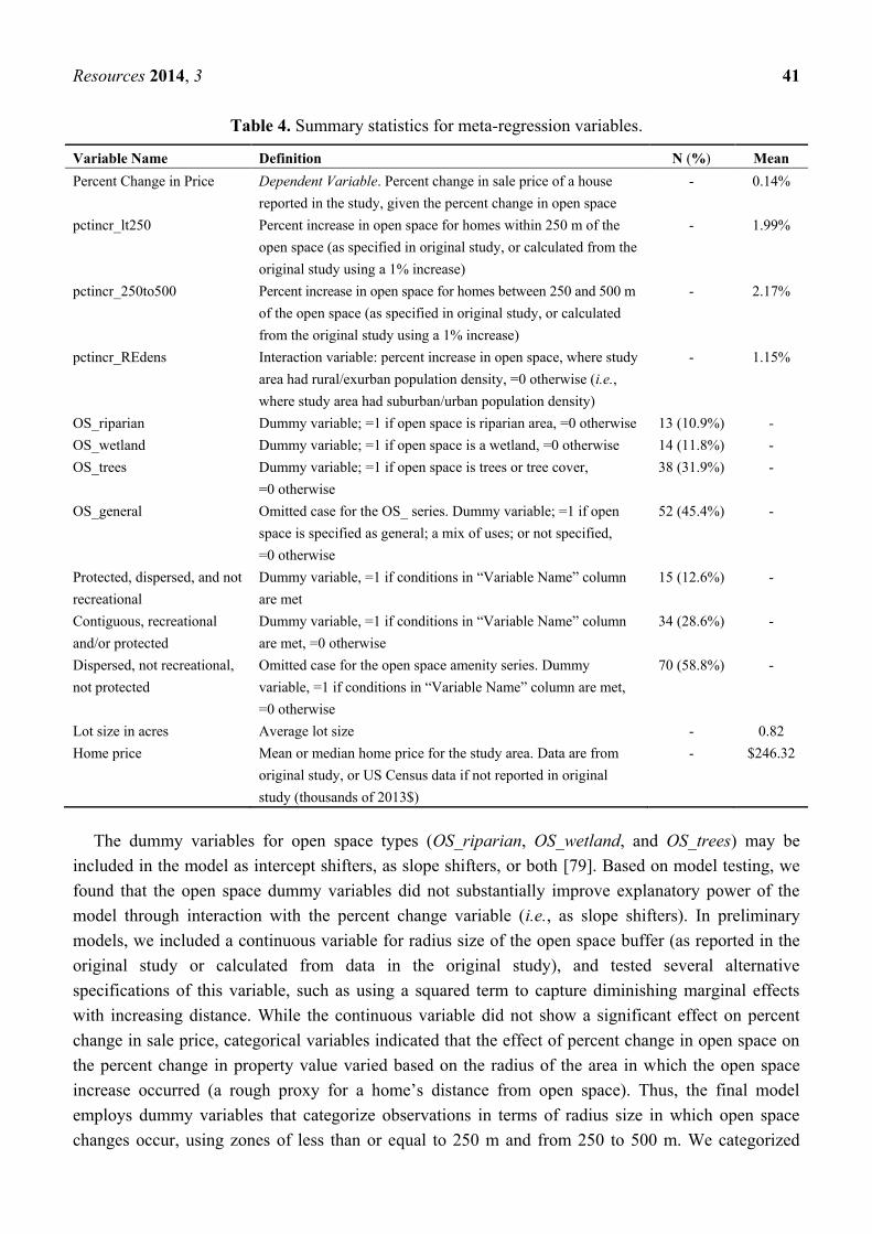
are discussed further below. Table 4 presents variable names, descriptions, and summary statistics for
the variables included in the final model.
Resources 2014, 3 41
Table 4. Summary statistics for meta-regression variables.
Variable Name Definition N (%) Mean
Percent Change in Price Dependent Variable. Percent change in sale price of a house
reported in the study, given the percent change in open space
- 0.14%
pctincr_lt250 Percent increase in open space for homes within 250 m of the
open space (as specified in original study, or calculated from the
original study using a 1% increase)
- 1.99%
pctincr_250to500 Percent increase in open space for homes between 250 and 500 m
of the open space (as specified in original study, or calculated
from the original study using a 1% increase)
- 2.17%
pctincr_REdens Interaction variable: percent increase in open space, where study
area had rural/exurban population density, =0 otherwise (i.e.,
where study area had suburban/urban population density)
- 1.15%
OS_riparian Dummy variable; =1 if open space is riparian area, =0 otherwise 13 (10.9%) -
OS_wetland Dummy variable; =1 if open space is a wetland, =0 otherwise 14 (11.8%) -
OS_trees Dummy variable; =1 if open space is trees or tree cover,
=0 otherwise
38 (31.9%) -
OS_general Omitted case for the OS_ series. Dummy variable; =1 if open
space is specified as general; a mix of uses; or not specified,
=0 otherwise
52 (45.4%) -
Protected, dispersed, and not
recreational
Dummy variable, =1 if conditions in “Variable Name” column
are met
15 (12.6%) -
Contiguous, recreational
and/or protected
Dummy variable, =1 if conditions in “Variable Name” column
are met, =0 otherwise
34 (28.6%) -
Dispersed, not recreational,
not protected
Omitted case for the open space amenity series. Dummy
variable, =1 if conditions in “Variable Name” column are met,
=0 otherwise
70 (58.8%) -
Lot size in acres Average lot size - 0.82
Home price Mean or median home price for the study area. Data are from
original study, or US Census data if not reported in original
study (thousands of 2013$)
- $246.32
The dummy variables for open space types (OS_riparian, OS_wetland, and OS_trees) may be
included in the model as intercept shifters, as slope shifters, or both [79]. Based on model testing, we
found that the open space dummy variables did not substantially improve explanatory power of the
model through interaction with the percent change variable (i.e., as slope shifters). In preliminary
models, we included a continuous variable for radius size of the open space buffer (as reported in the
original study or calculated from data in the original study), and tested several alternative
specifications of this variable, such as using a squared term to capture diminishing marginal effects
with increasing distance. While the continuous variable did not show a significant effect on percent
change in sale price, categorical variables indicated that the effect of percent change in open space on
the percent change in property value varied based on the radius of the area in which the open space
increase occurred (a rough proxy for a home’s distance from open space). Thus, the final model
employs dummy variables that categorize observations in terms of radius size in which open space
changes occur, using zones of less than or equal to 250 m and from 250 to 500 m. We categorized
Resources 2014, 3 42
study data by zone using information from the original studies (see Table 3). The smallest zone, where
open space increases are evaluated within a 250 m radius, captures properties with on-site or adjacent
open spaces and properties with off-site open space within 250 m. The subsequent buffer area, from
250 to 500 m in distance, roughly corresponds to both the mean radius in the final sample of studies
(583 m, range 15–5391 m), and to a generally accepted quarter-mile distance threshold for “walkability”
between residences and open space destinations [80]. Preliminary models including larger radius
buffers suggested open space increases of the type and size evaluated in our model and in radius zones
larger than 500 meters were not reflected in property values.
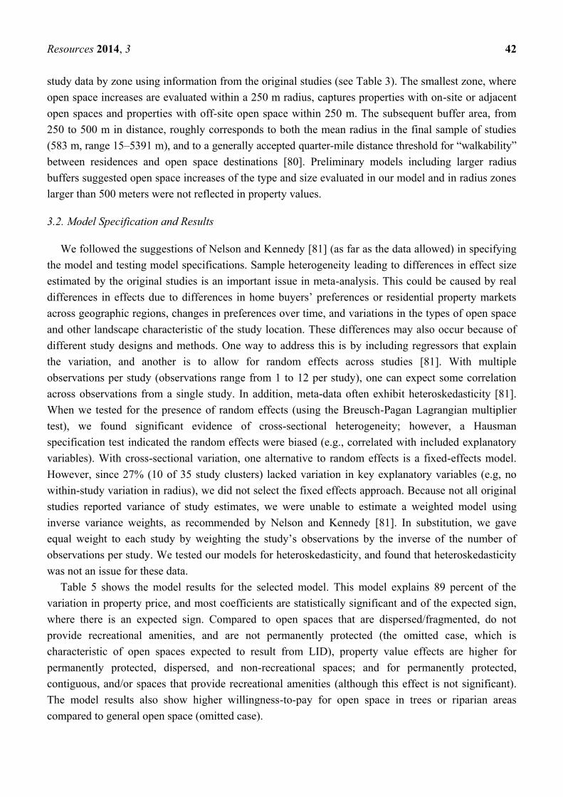
3.2. Model Specification and Results
We followed the suggestions of Nelson and Kennedy [81] (as far as the data allowed) in specifying
the model and testing model specifications. Sample heterogeneity leading to differences in effect size
estimated by the original studies is an important issue in meta-analysis. This could be caused by real
differences in effects due to differences in home buyers’ preferences or residential property markets
across geographic regions, changes in preferences over time, and variations in the types of open space
and other landscape characteristic of the study location. These differences may also occur because of
different study designs and methods. One way to address this is by including regressors that explain
the variation, and another is to allow for random effects across studies [81]. With multiple
observations per study (observations range from 1 to 12 per study), one can expect some correlation
across observations from a single study. In addition, meta-data often exhibit heteroskedasticity [81].
When we tested for the presence of random effects (using the Breusch-Pagan Lagrangian multiplier
test), we found significant evidence of cross-sectional heterogeneity; however, a Hausman
specification test indicated the random effects were biased (e.g., correlated with included explanatory
variables). With cross-sectional variation, one alternative to random effects is a fixed-effects model.
However, since 27% (10 of 35 study clusters) lacked variation in key explanatory variables (e.g, no
within-study variation in radius), we did not select the fixed effects approach. Because not all original
studies reported variance of study estimates, we were unable to estimate a weighted model using
inverse variance weights, as recommended by Nelson and Kennedy [81]. In substitution, we gave
equal weight to each study by weighting the study’s observations by the inverse of the number of
observations per study. We tested our models for heteroskedasticity, and found that heteroskedasticity
was not an issue for these data.
Table 5 shows the model results for the selected model. This model explains 89 percent of the
variation in property price, and most coefficients are statistically significant and of the expected sign,
where there is an expected sign. Compared to open spaces that are dispersed/fragmented, do not
provide recreational amenities, and are not permanently protected (the omitted case, which is
characteristic of open spaces expected to result from LID), property value effects are higher for
permanently protected, dispersed, and non-recreational spaces; and for permanently protected,
contiguous, and/or spaces that provide recreational amenities (although this effect is not significant).
The model results also show higher willingness-to-pay for open space in trees or riparian areas
compared to general open space (omitted case).

Resources 2014, 3 43
We captured the effect of distance from open space improvements on property price by using two
interaction variables between buffer size categories (0–250 m. and 250–500 m) and the percent
increase in open space. Coefficients on these variables illustrate a diminishing marginal effect of a
percent increase in open space as distance of the buffer increases. A percentage increase in open space
is valued less in rural and exurban population density areas compared to suburban and urban density
areas. Prior studies have found that wetlands, trees, and riparian areas elicit inconsistent effects on
property values, including negative, positive, and zero effects (e.g., reviewed in [14]). The coefficient
on wetlands is not significant, indicating that the value of open space that is wetlands is not
significantly different from that of the general open space category. Several factors may contribute to
the identified overall positive effect of trees and riparian areas in this model including:
(1) observations from studies evaluating the effect of open space providing high-quality wildlife and
bird habitat; and (2) the study-weighting approach, which gave higher weight to observations which
came from studies with fewer meta-data observations.
The negative coefficient for the log of lot size indicates that, all else equal, homes with larger lots
will have a smaller percent change in price when open space increases. This provides weak support for
the hypothesis of a tradeoff between lot size and open space size. However, the coefficient is not
significant. The coefficient on home price is negative and significant, though extremely small. This
implies that homes with higher values will have a slightly smaller price response to an increase in
nearby open space, as compared to lower-valued homes.
Table 5. Linear weighted regression: % change in willingness to pay (WTP).
Variable Parameter Estimate Standard Error
Intercept 0.039 0.079
pctincr_lt250 0.169*** 0.006
pctincr_250to500 0.102*** 0.005
pctincr_REdens −0.063** 0.020
OS_ trees1 0.245*** 0.065
OS_ riparian1 0.252* 0.117
OS_ wetland1 −0.013 0.084
Protected, dispersed, and not recreational2 0.392*** 0.074
Contiguous, recreational and/or protected2 0.081 0.067
Ln(lot size in acres) −0.018 0.025
Home price ($thousands) −0.0009*** 2.48 × 10⁻⁷
Notes: F10,108 = 165, p < 0.0001; Number of observations = 119; Adjusted R2 = 0.93; Number of studies = 35;
*: Significant at the 0.05 level; **: Significant at the 0.01 level; ***: Significant at the 0.001 level; 1: Base
case for vegetation type is “general” (i.e., various types, undefined, or vegetated but not primarily
tree-covered) open space; 2: Base case for open space category is dispersed, not protected, not recreational.
3.3. Tests for Robustness of Parameter Estimates
We followed a set of procedures for testing robustness of the model’s parameter estimates
suggested by Boyle, et al. [30]. In addition to the study selection procedure discussed in Section 2,
above, we tested for sample selection bias, horizontal robustness (inclusion/exclusion of observations
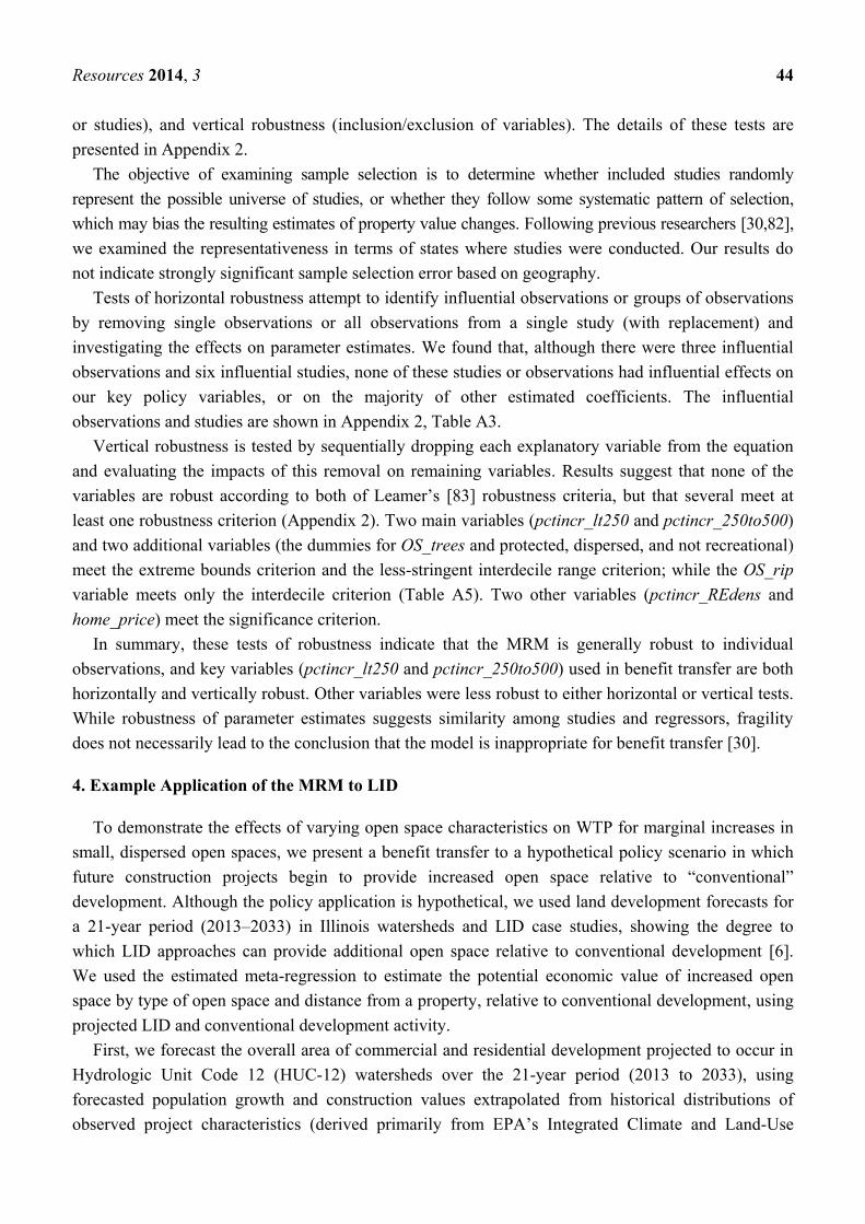
Resources 2014, 3 44
or studies), and vertical robustness (inclusion/exclusion of variables). The details of these tests are
presented in Appendix 2.
The objective of examining sample selection is to determine whether included studies randomly
represent the possible universe of studies, or whether they follow some systematic pattern of selection,
which may bias the resulting estimates of property value changes. Following previous researchers [30,82],
we examined the representativeness in terms of states where studies were conducted. Our results do
not indicate strongly significant sample selection error based on geography.
Tests of horizontal robustness attempt to identify influential observations or groups of observations
by removing single observations or all observations from a single study (with replacement) and
investigating the effects on parameter estimates. We found that, although there were three influential
observations and six influential studies, none of these studies or observations had influential effects on
our key policy variables, or on the majority of other estimated coefficients. The influential
observations and studies are shown in Appendix 2, Table A3.
Vertical robustness is tested by sequentially dropping each explanatory variable from the equation
and evaluating the impacts of this removal on remaining variables. Results suggest that none of the
variables are robust according to both of Leamer’s [83] robustness criteria, but that several meet at
least one robustness criterion (Appendix 2). Two main variables (pctincr_lt250 and pctincr_250to500)
and two additional variables (the dummies for OS_trees and protected, dispersed, and not recreational)
meet the extreme bounds criterion and the less-stringent interdecile range criterion; while the OS_rip
variable meets only the interdecile criterion (Table A5). Two other variables (pctincr_REdens and
home_price) meet the significance criterion.
In summary, these tests of robustness indicate that the MRM is generally robust to individual
observations, and key variables (pctincr_lt250 and pctincr_250to500) used in benefit transfer are both
horizontally and vertically robust. Other variables were less robust to either horizontal or vertical tests.
While robustness of parameter estimates suggests similarity among studies and regressors, fragility
does not necessarily lead to the conclusion that the model is inappropriate for benefit transfer [30].
4. Example Application of the MRM to LID
To demonstrate the effects of varying open space characteristics on WTP for marginal increases in
small, dispersed open spaces, we present a benefit transfer to a hypothetical policy scenario in which
future construction projects begin to provide increased open space relative to “conventional”
development. Although the policy application is hypothetical, we used land development forecasts for
a 21-year period (2013–2033) in Illinois watersheds and LID case studies, showing the degree to
which LID approaches can provide additional open space relative to conventional development [6].
We used the estimated meta-regression to estimate the potential economic value of increased open
space by type of open space and distance from a property, relative to conventional development, using
projected LID and conventional development activity.
First, we forecast the overall area of commercial and residential development projected to occur in
Hydrologic Unit Code 12 (HUC-12) watersheds over the 21-year period (2013 to 2033), using
forecasted population growth and construction values extrapolated from historical distributions of
observed project characteristics (derived primarily from EPA’s Integrated Climate and Land-Use
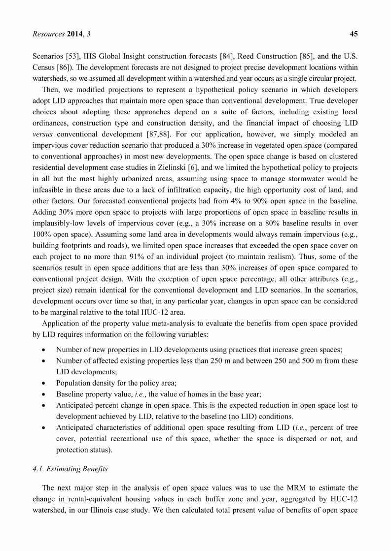
Resources 2014, 3 45
Scenarios [53], IHS Global Insight construction forecasts [84], Reed Construction [85], and the U.S.
Census [86]). The development forecasts are not designed to project precise development locations within
watersheds, so we assumed all development within a watershed and year occurs as a single circular project.
Then, we modified projections to represent a hypothetical policy scenario in which developers
adopt LID approaches that maintain more open space than conventional development. True developer
choices about adopting these approaches depend on a suite of factors, including existing local
ordinances, construction type and construction density, and the financial impact of choosing LID
versus conventional development [87,88]. For our application, however, we simply modeled an
impervious cover reduction scenario that produced a 30% increase in vegetated open space (compared
to conventional approaches) in most new developments. The open space change is based on clustered
residential development case studies in Zielinski [6], and we limited the hypothetical policy to projects
in all but the most highly urbanized areas, assuming using space to manage stormwater would be
infeasible in these areas due to a lack of infiltration capacity, the high opportunity cost of land, and
other factors. Our forecasted conventional projects had from 4% to 90% open space in the baseline.
Adding 30% more open space to projects with large proportions of open space in baseline results in
implausibly-low levels of impervious cover (e.g., a 30% increase on a 80% baseline results in over
100% open space). Assuming some land area in developments would always remain impervious (e.g.,
building footprints and roads), we limited open space increases that exceeded the open space cover on
each project to no more than 91% of an individual project (to maintain realism). Thus, some of the
scenarios result in open space additions that are less than 30% increases of open space compared to
conventional project design. With the exception of open space percentage, all other attributes (e.g.,
project size) remain identical for the conventional development and LID scenarios. In the scenarios,
development occurs over time so that, in any particular year, changes in open space can be considered
to be marginal relative to the total HUC-12 area.
Application of the property value meta-analysis to evaluate the benefits from open space provided
by LID requires information on the following variables:
Number of new properties in LID developments using practices that increase green spaces;
Number of affected existing properties less than 250 m and between 250 and 500 m from these
LID developments;
Population density for the policy area;
Baseline property value, i.e., the value of homes in the base year;
Anticipated percent change in open space. This is the expected reduction in open space lost to
development achieved by LID, relative to the baseline (no LID) conditions.
Anticipated characteristics of additional open space resulting from LID (i.e., percent of tree
cover, potential recreational use of this space, whether the space is dispersed or not, and
protection status).
4.1. Estimating Benefits
The next major step in the analysis of open space values was to use the MRM to estimate the
change in rental-equivalent housing values in each buffer zone and year, aggregated by HUC-12
watershed, in our Illinois case study. We then calculated total present value of benefits of open space
Resources 2014, 3 46
by summing the present discounted values of these benefit flows. The following sub-sections describe
these calculations in more detail.
4.1.1. Benefit Transfer Based on Meta-Analysis Regression
We used the MRM to estimate the percentage change in annualized rental-equivalent property values
given changes in LID open space (relative to conventional development) in each HUC-12, project, buffer
zone, and year. The general approach follows standard methods illustrated by Shrestha et al. [34] and
Bergstrom & Taylor [32], among many others [89]. The estimated MRM allows us to forecast the
increase in the annual rental value of a property based on model variables that represent percentage
changes in open space under the LID scenario, radius size, characteristics of the open space valued,
and population density.
The meta-analysis uses a simple benefit function of the following general form:
i i%Δ(HomePrice) Intercept Coefficient Independent Variable (1)
Here, the dependent variable %Δ(HomePrice) represents the percent change in price of a home. The
MRM can be also used predict percentage changes in the annual rental-equivalent value of a home
since the price of a home is simply the sum of the discounted future annual rental-equivalent values of
living in that home [90–93]. We estimated the annual rental-equivalent home value by first calculating
the average current value per home for each HUC-12, and then converting the aggregate housing
values to annual rental-equivalent housing values by multiplying housing values (for each distance
buffer, year, and HUC-12) by a 3% discount rate [94]. The average current home value for a given
watershed is estimated as a weighted average of the present-day median home values in all Census
tracts intersecting the HUC-12 (using American Community Survey 5-year estimates [95]). The
current home value in the HUC-12 watersheds with predicted new and re-development was $151,875,
translating to an average annual rental value (at a 3% discount rate) of $4556. Although real housing
prices do vary considerably over time, long term price trends are difficult to predict [96], and
predicting trends in home values is beyond the scope of this study.
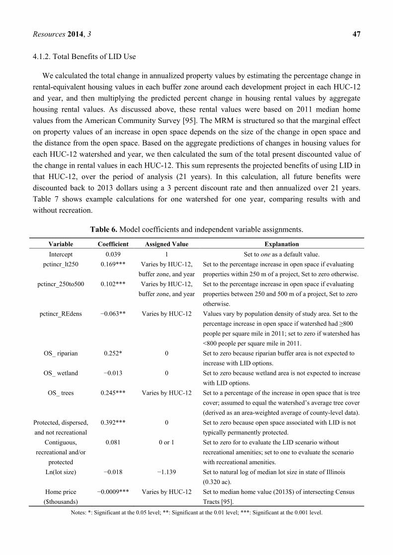
We assigned a value to each model variable based on the policy context and the social and
environmental characteristics (e.g., percent tree cover, population density) of each HUC-12, project,
distance buffer, and year. Table 6 presents the variables, estimated coefficients, assigned variable
values, and explanations for assigned values that vary across locations. We assumed that (1) additional
open spaces associated with LID would be dispersed and unprotected areas comprised of either trees or
general vegetation; and (2) relative tree cover at developments would vary regionally and consistently
with nearby developed areas. The area-weighted average percent tree cover for each watershed was
estimated based on the National Land Cover Database (NLCD) 2001 [97] tree canopy data for areas
with developed land use types, using county-level summary tables generated by the U.S. Forest
Service [98]. To evaluate the incremental value of recreational amenities provided by LID, we
considered land development scenarios with and without recreational amenities.
Resources 2014, 3 47
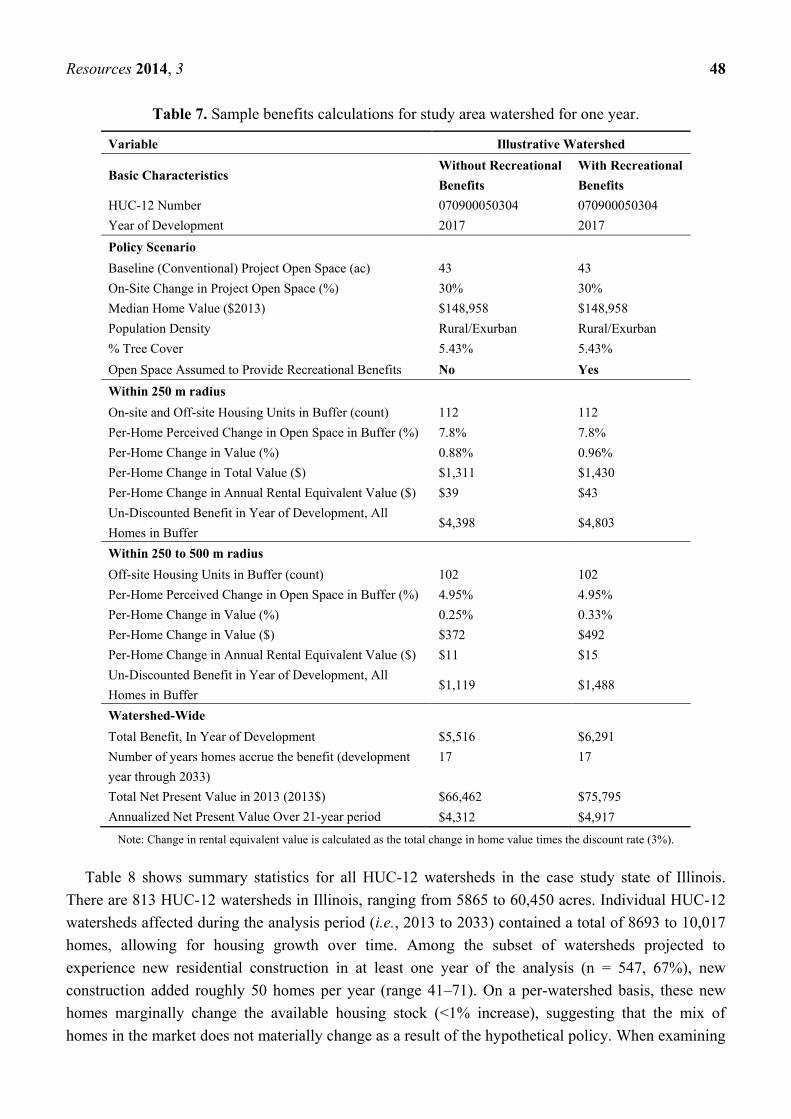
4.1.2. Total Benefits of LID Use
We calculated the total change in annualized property values by estimating the percentage change in
rental-equivalent housing values in each buffer zone around each development project in each HUC-12
and year, and then multiplying the predicted percent change in housing rental values by aggregate
housing rental values. As discussed above, these rental values were based on 2011 median home
values from the American Community Survey [95]. The MRM is structured so that the marginal effect
on property values of an increase in open space depends on the size of the change in open space and
the distance from the open space. Based on the aggregate predictions of changes in housing values for
each HUC-12 watershed and year, we then calculated the sum of the total present discounted value of
the change in rental values in each HUC-12. This sum represents the projected benefits of using LID in
that HUC-12, over the period of analysis (21 years). In this calculation, all future benefits were
discounted back to 2013 dollars using a 3 percent discount rate and then annualized over 21 years.
Table 7 shows example calculations for one watershed for one year, comparing results with and
without recreation.
Table 6. Model coefficients and independent variable assignments.
Variable Coefficient Assigned Value Explanation
Intercept 0.039 1 Set to one as a default value.
pctincr_lt250 0.169*** Varies by HUC-12,
buffer zone, and year
Set to the percentage increase in open space if evaluating
properties within 250 m of a project, Set to zero otherwise.
pctincr_250to500 0.102*** Varies by HUC-12,
buffer zone, and year
Set to the percentage increase in open space if evaluating
properties between 250 and 500 m of a project, Set to zero
otherwise.
pctincr_REdens −0.063** Varies by HUC-12 Values vary by population density of study area. Set to the
percentage increase in open space if watershed had ≥800
people per square mile in 2011; set to zero if watershed has
<800 people per square mile in 2011.
OS_ riparian 0.252* 0 Set to zero because riparian buffer area is not expected to
increase with LID options.
OS_ wetland −0.013 0 Set to zero because wetland area is not expected to increase
with LID options.
OS_ trees 0.245*** Varies by HUC-12 Set to a percentage of the increase in open space that is tree
cover; assumed to equal the watershed’s average tree cover
(derived as an area-weighted average of county-level data).
Protected, dispersed,
and not recreational
0.392*** 0 Set to zero because open space associated with LID is not
typically permanently protected.
Contiguous,
recreational and/or
protected
0.081 0 or 1 Set to zero for to evaluate the LID scenario without
recreational amenities; set to one to evaluate the scenario
with recreational amenities.
Ln(lot size) −0.018 −1.139 Set to natural log of median lot size in state of Illinois
(0.320 ac).
Home price
($thousands)
−0.0009*** Varies by HUC-12 Set to median home value (2013$) of intersecting Census
Tracts [95].
Notes: *: Significant at the 0.05 level; **: Significant at the 0.01 level; ***: Significant at the 0.001 level.
Resources 2014, 3 48
Table 7. Sample benefits calculations for study area watershed for one year.
Variable Illustrative Watershed
Basic Characteristics Without Recreational
Benefits
With Recreational
Benefits
HUC-12 Number 070900050304 070900050304
Year of Development 2017 2017
Policy Scenario
Baseline (Conventional) Project Open Space (ac) 43 43
On-Site Change in Project Open Space (%) 30% 30%
Median Home Value ($2013) $148,958 $148,958
Population Density Rural/Exurban Rural/Exurban
% Tree Cover 5.43% 5.43%
Open Space Assumed to Provide Recreational Benefits No Yes
Within 250 m radius
On-site and Off-site Housing Units in Buffer (count) 112 112
Per-Home Perceived Change in Open Space in Buffer (%) 7.8% 7.8%
Per-Home Change in Value (%) 0.88% 0.96%
Per-Home Change in Total Value ($) $1,311 $1,430
Per-Home Change in Annual Rental Equivalent Value ($) $39 $43
Un-Discounted Benefit in Year of Development, All
Homes in Buffer $4,398 $4,803
Within 250 to 500 m radius
Off-site Housing Units in Buffer (count) 102 102
Per-Home Perceived Change in Open Space in Buffer (%) 4.95% 4.95%
Per-Home Change in Value (%) 0.25% 0.33%
Per-Home Change in Value ($) $372 $492
Per-Home Change in Annual Rental Equivalent Value ($) $11 $15
Un-Discounted Benefit in Year of Development, All
Homes in Buffer $1,119 $1,488
Watershed-Wide
Total Benefit, In Year of Development $5,516 $6,291
Number of years homes accrue the benefit (development
year through 2033)
17 17
Total Net Present Value in 2013 (2013$) $66,462 $75,795
Annualized Net Present Value Over 21-year period $4,312 $4,917
Note: Change in rental equivalent value is calculated as the total change in home value times the discount rate (3%).
Table 8 shows summary statistics for all HUC-12 watersheds in the case study state of Illinois.
There are 813 HUC-12 watersheds in Illinois, ranging from 5865 to 60,450 acres. Individual HUC-12
watersheds affected during the analysis period (i.e., 2013 to 2033) contained a total of 8693 to 10,017
homes, allowing for housing growth over time. Among the subset of watersheds projected to
experience new residential construction in at least one year of the analysis (n = 547, 67%), new
construction added roughly 50 homes per year (range 41–71). On a per-watershed basis, these new
homes marginally change the available housing stock (<1% increase), suggesting that the mix of
homes in the market does not materially change as a result of the hypothetical policy. When examining
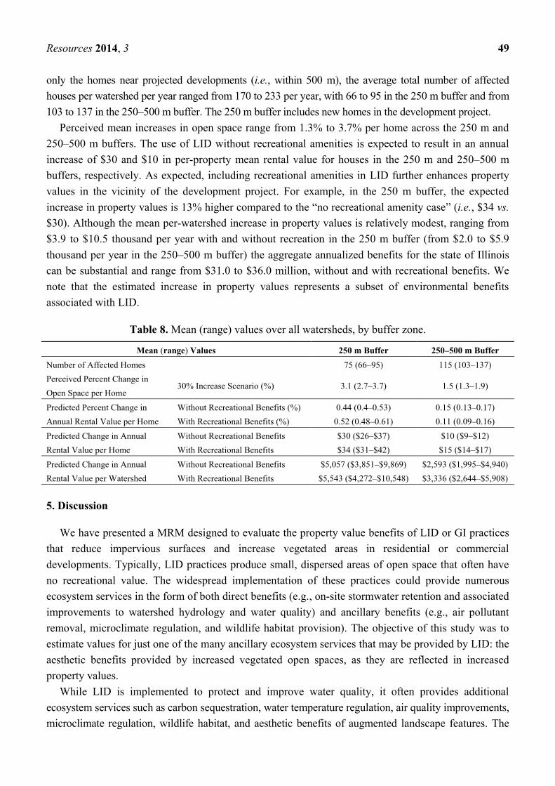
Resources 2014, 3 49
only the homes near projected developments (i.e., within 500 m), the average total number of affected
houses per watershed per year ranged from 170 to 233 per year, with 66 to 95 in the 250 m buffer and from
103 to 137 in the 250–500 m buffer. The 250 m buffer includes new homes in the development project.
Perceived mean increases in open space range from 1.3% to 3.7% per home across the 250 m and
250–500 m buffers. The use of LID without recreational amenities is expected to result in an annual
increase of $30 and $10 in per-property mean rental value for houses in the 250 m and 250–500 m
buffers, respectively. As expected, including recreational amenities in LID further enhances property
values in the vicinity of the development project. For example, in the 250 m buffer, the expected
increase in property values is 13% higher compared to the “no recreational amenity case” (i.e., $34 vs.
$30). Although the mean per-watershed increase in property values is relatively modest, ranging from
$3.9 to $10.5 thousand per year with and without recreation in the 250 m buffer (from $2.0 to $5.9
thousand per year in the 250–500 m buffer) the aggregate annualized benefits for the state of Illinois
can be substantial and range from $31.0 to $36.0 million, without and with recreational benefits. We
note that the estimated increase in property values represents a subset of environmental benefits
associated with LID.
Table 8. Mean (range) values over all watersheds, by buffer zone.
Mean (range) Values 250 m Buffer 250–500 m Buffer
Number of Affected Homes 75 (66–95) 115 (103–137)
Perceived Percent Change in
Open Space per Home 30% Increase Scenario (%) 3.1 (2.7–3.7) 1.5 (1.3–1.9)
Predicted Percent Change in
Annual Rental Value per Home
Without Recreational Benefits (%) 0.44 (0.4–0.53) 0.15 (0.13–0.17)
With Recreational Benefits (%) 0.52 (0.48–0.61) 0.11 (0.09–0.16)
Predicted Change in Annual
Rental Value per Home
Without Recreational Benefits $30 ($26–$37) $10 ($9–$12)
With Recreational Benefits $34 ($31–$42) $15 ($14–$17)
Predicted Change in Annual
Rental Value per Watershed
Without Recreational Benefits $5,057 ($3,851–$9,869) $2,593 ($1,995–$4,940)
With Recreational Benefits $5,543 ($4,272–$10,548) $3,336 ($2,644–$5,908)
5. Discussion
We have presented a MRM designed to evaluate the property value benefits of LID or GI practices
that reduce impervious surfaces and increase vegetated areas in residential or commercial
developments. Typically, LID practices produce small, dispersed areas of open space that often have
no recreational value. The widespread implementation of these practices could provide numerous
ecosystem services in the form of both direct benefits (e.g., on-site stormwater retention and associated
improvements to watershed hydrology and water quality) and ancillary benefits (e.g., air pollutant
removal, microclimate regulation, and wildlife habitat provision). The objective of this study was to
estimate values for just one of the many ancillary ecosystem services that may be provided by LID: the
aesthetic benefits provided by increased vegetated open spaces, as they are reflected in increased
property values.
While LID is implemented to protect and improve water quality, it often provides additional
ecosystem services such as carbon sequestration, water temperature regulation, air quality improvements,
microclimate regulation, wildlife habitat, and aesthetic benefits of augmented landscape features. The

Resources 2014, 3 50
improved ecosystem services, in particular augmented landscape features, may be reflected in
increased property values.
We developed and estimated a MRM with 119 observations from 35 studies, including only studies
that are most relevant to the small, dispersed types of open space likely to result from LID. Because
our model is intended for use in benefit transfer, our analysis included robustness tests [30]. Based on
robustness tests, we conclude that neither national research priorities nor our choices in selecting a
subset of studies for an analysis of small, dispersed spaces appear to bias conclusions drawn from our
meta-analysis. The estimated MRM is generally robust to individual observations, and key variables
used in benefit transfer—those describing the percent change in open space at different distances—are
both horizontally and vertically robust. Overall, we are confident that value transfer based on this
equation is as accurate as possible, given underlying data, but do recommend caution in interpreting
results based on the less-robust variables.
Our benefit transfer example, which illustrated the application of the meta-analysis function to a
hypothetical policy scenario, wherein new developments in Illinois watersheds are constructed with up
to 30% more open space as compared to conventional development, illustrated the utility of using a
meta-analysis function that can tailor value estimates to site-specific changes. Nevertheless, the benefit
transfer exercise also demonstrates that relatively small benefits arise from increases in small,
dispersed open spaces, such as those typical of some LID options. This is to be expected, as some of
the more conservative LID approaches, such as reducing street width, produce marginal changes in
open space. However, when evaluated over many developments, and when combined with the
numerous other benefits that may be provided by low impact development (e.g., improved watershed
hydrology and air pollution removal by vegetation), our results suggest landscape-wide amenity values
of LID can be significant. Some developers use LID that provides additional open space areas for
recreation [5,41]. We compared the results of our model when evaluating sites with recreational uses
to sites without recreational uses, and found that on-site and nearby off-site homeowners may value
LID plans that use contiguous blocks of open space that provide recreational amenities more than
those which do not provide these features.
Like prior meta-analyses based on hedonic price equations [42,99], we examined insights from
multiple real estate markets across the United States. This enabled us to comment broadly on the
average relationship between open space and property values. Nonetheless, our final meta-regression
did not include region-specific effects due to small sample sizes. While regional dummy variables
would have allowed practitioners to coarsely tailor our national results to specific geographic contexts,
we recommend using other variables in the regression, such as local tree cover and open space types
pertinent to local contexts.
Our results indicate that the design and characteristics of a project affect the magnitude of benefits,
and that values decline with distance. More broadly, the meta-analysis shows that the percent increase
in open space and proximity are robust determinants of household WTP for aesthetic and other
services associated with local availability of small, dispersed open spaces, but that values for other site
features (e.g., tree cover or recreational use) may be site-specific. Policymakers and developers could
draw on our synthesis of the property value effects of various site characteristics to maximize benefits
from open space associated with LID. We, however, note that while changes in property values capture

Resources 2014, 3 51
a portion of the net benefits of LID, they may not address the full suite of LID benefits (e.g., energy
savings from improved house shading).
Acknowledgments
The authors acknowledge helpful comments from Denny Guignet, Matt Ranson, Mike Papenfus,
Erik Helm, and Todd Doley, and from three anonymous reviewers. This research was funded by U.S.
EPA Contract No. EP-C-07-023 to Abt Associates. This is also contribution number ORD-005034 of
the Atlantic Ecology Division, National Health and Environmental Effects Research Laboratory,
Office of Research and Development, U. S. Environmental Protection Agency. This study has not been
subjected to Agency review. Therefore, the findings, conclusions, and views expressed here are those
of the authors and do not necessarily reflect those of the U.S. EPA. No official Agency endorsement
should be inferred.
Conflicts of Interest
The authors declare no conflict of interest.
Appendix 1: Methodology to Convert Distance from Open Space and Adjacency to Open Space
to Percent Changes in Open Space
1.1. Converting Distance to Percent
The conversion of a home’s distance to nearby open space features into the percentage of open
space in a buffer surrounding a home proceeds in several conceptual steps [43]. First, we drew a
circular buffer area around homes, with a radius equal to the baseline average distance between homes
in the study and the nearest open space feature. In the baseline, open space features abut but do not
overlap the perimeter of the home buffer (Figure A1a). We simulate a reduction in the distance
between homes and open space by “moving” the open space from its original position to one which
overlaps the home buffer (Figure A1b). Open space is “moved” closer to the home by the mean change
in distance examined in the original study. Then, we calculated the resulting percent increase in open
space within the home buffer as the ratio of the area of overlap to the total area of the home buffer.
Figure A1. Conceptual illustration of converting distance-based measures to
percent-based measures. (a) Open space abutting the buffer; (b) Open space “moved” to
overlap the buffer.
(a)
(b)
Resources 2014, 3 52
1.2. Converting Adjacency to Percent
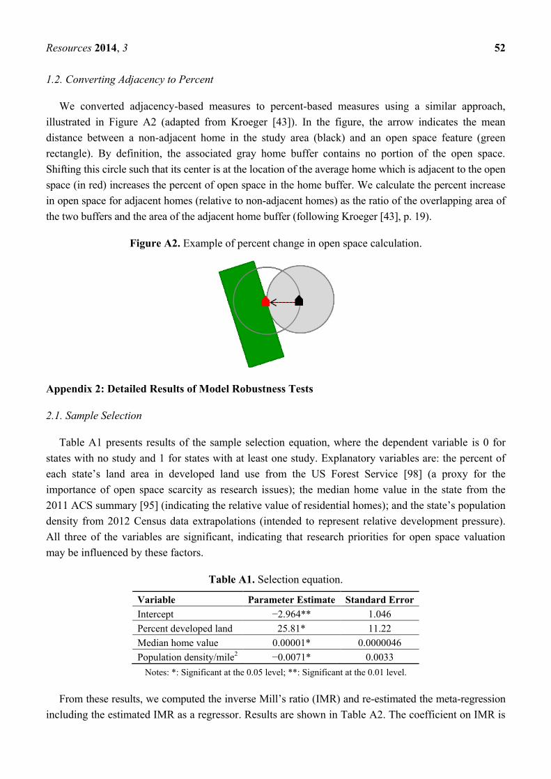
We converted adjacency-based measures to percent-based measures using a similar approach,
illustrated in Figure A2 (adapted from Kroeger [43]). In the figure, the arrow indicates the mean
distance between a non-adjacent home in the study area (black) and an open space feature (green
rectangle). By definition, the associated gray home buffer contains no portion of the open space.
Shifting this circle such that its center is at the location of the average home which is adjacent to the open
space (in red) increases the percent of open space in the home buffer. We calculate the percent increase
in open space for adjacent homes (relative to non-adjacent homes) as the ratio of the overlapping area of
the two buffers and the area of the adjacent home buffer (following Kroeger [43], p. 19).
Figure A2. Example of percent change in open space calculation.
Appendix 2: Detailed Results of Model Robustness Tests
2.1. Sample Selection
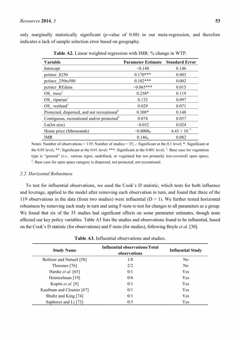
Table A1 presents results of the sample selection equation, where the dependent variable is 0 for
states with no study and 1 for states with at least one study. Explanatory variables are: the percent of
each state’s land area in developed land use from the US Forest Service [98] (a proxy for the
importance of open space scarcity as research issues); the median home value in the state from the
2011 ACS summary [95] (indicating the relative value of residential homes); and the state’s population
density from 2012 Census data extrapolations (intended to represent relative development pressure).
All three of the variables are significant, indicating that research priorities for open space valuation
may be influenced by these factors.
Table A1. Selection equation.
Variable Parameter Estimate Standard Error
Intercept −2.964** 1.046
Percent developed land 25.81* 11.22
Median home value 0.00001* 0.0000046
Population density/mile2 −0.0071* 0.0033
Notes: *: Significant at the 0.05 level; **: Significant at the 0.01 level.
From these results, we computed the inverse Mill’s ratio (IMR) and re-estimated the meta-regression
including the estimated IMR as a regressor. Results are shown in Table A2. The coefficient on IMR is
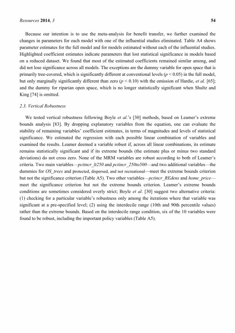
Resources 2014, 3 53
only marginally statistically significant (p-value of 0.08) in our meta-regression, and therefore
indicates a lack of sample selection error based on geography.
Table A2. Linear weighted regression with IMR: % change in WTP.
Variable Parameter Estimate Standard Error
Intercept −0.148 0.146
pctincr_lt250 0.170*** 0.003
pctincr_250to500 0.102*** 0.002
pctincr_REdens −0.065*** 0.015
OS_ trees1 0.258* 0.119
OS_ riparian1 0.132 0.097
OS_ wetland1 0.029 0.071
Protected, dispersed, and not recreational2 0.308* 0.148
Contiguous, recreational and/or protected2 0.074 0.057
Ln(lot size) −0.032 0.024
Home price ($thousands) −0.0008. 4.43 × 10⁻⁷
IMR 0.146. 0.082
Notes: Number of observations = 119; Number of studies = 35; .: Significant at the 0.1 level; *: Significant at
the 0.05 level; **: Significant at the 0.01 level; ***: Significant at the 0.001 level; 1: Base case for vegetation
type is “general” (i.e., various types, undefined, or vegetated but not primarily tree-covered) open space; 2: Base case for open space category is dispersed, not protected, not recreational.
2.2. Horizontal Robustness
To test for influential observations, we used the Cook’s D statistic, which tests for both influence
and leverage, applied to the model after removing each observation in turn, and found that three of the
119 observations in the data (from two studies) were influential (D > 1). We further tested horizontal
robustness by removing each study in turn and using F-tests to test for changes to all parameters as a group.
We found that six of the 35 studies had significant effects on some parameter estimates, though none
affected our key policy variables. Table A3 lists the studies and observations found to be influential, based
on the Cook’s D statistic (for observations) and F-tests (for studies), following Boyle et al. [30].
Table A3. Influential observations and studies.
Study Name Influential observations/Total
observations Influential Study
Bolitzer and Netusil [58] 1/8 No
Thorsnes [76] 2/2 No
Hardie et al. [65] 0/1 Yes
Heintzelman [19] 0/6 Yes
Kopits et al. [9] 0/1 Yes
Kaufman and Cloutier [67] 0/1 Yes
Shultz and King [74] 0/1 Yes
Saphores and Li [73] 0/3 Yes
Resources 2014, 3 54
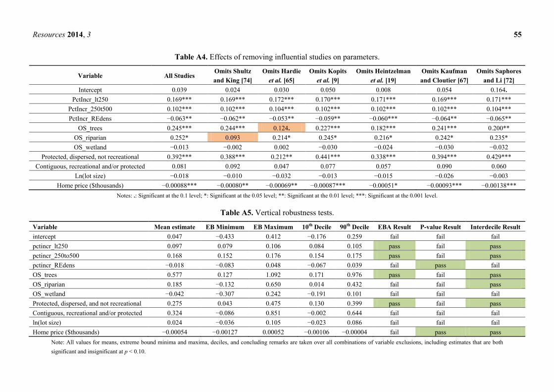
Because our intention is to use the meta-analysis for benefit transfer, we further examined the
changes in parameters for each model with one of the influential studies eliminated. Table A4 shows
parameter estimates for the full model and for models estimated without each of the influential studies.
Highlighted coefficient estimates indicate parameters that lost statistical significance in models based
on a reduced dataset. We found that most of the estimated coefficients remained similar among, and
did not lose significance across all models. The exceptions are the dummy variable for open space that is
primarily tree-covered, which is significantly different at conventional levels (p < 0.05) in the full model,
but only marginally significantly different than zero (p < 0.10) with the omission of Hardie, et al. [65];
and the dummy for riparian open space, which is no longer statistically significant when Shultz and
King [74] is omitted.
2.3. Vertical Robustness
We tested vertical robustness following Boyle et al.’s [30] methods, based on Leamer’s extreme
bounds analysis [83]. By dropping explanatory variables from the equation, one can evaluate the
stability of remaining variables’ coefficient estimates, in terms of magnitudes and levels of statistical
significance. We estimated the regression with each possible linear combination of variables and
examined the results. Leamer deemed a variable robust if, across all linear combinations, its estimate
remains statistically significant and if its extreme bounds (the estimate plus or minus two standard
deviations) do not cross zero. None of the MRM variables are robust according to both of Leamer’s
criteria. Two main variables—pctincr_lt250 and pctincr_250to500—and two additional variables—the
dummies for OS_trees and protected, dispersed, and not recreational—meet the extreme bounds criterion
but not the significance criterion (Table A5). Two other variables—pctincr_REdens and home_price—
meet the significance criterion but not the extreme bounds criterion. Leamer’s extreme bounds
conditions are sometimes considered overly strict; Boyle et al. [30] suggest two alternative criteria:
(1) checking for a particular variable’s robustness only among the iterations where that variable was
significant at a pre-specified level; (2) using the interdecile range (10th and 90th percentile values)
rather than the extreme bounds. Based on the interdecile range condition, six of the 10 variables were
found to be robust, including the important policy variables (Table A5).
Resources 2014, 3 55
Table A4. Effects of removing influential studies on parameters.
Variable All Studies Omits Shultz
and King [74]
Omits Hardie
et al. [65]
Omits Kopits
et al. [9]
Omits Heintzelman
et al. [19]
Omits Kaufman
and Cloutier [67]
Omits Saphores
and Li [72]
Intercept 0.039 0.024 0.030 0.050 0.008 0.054 0.164.
PctIncr_lt250 0.169*** 0.169*** 0.172*** 0.170*** 0.171*** 0.169*** 0.171***
PctIncr_250t500 0.102*** 0.102*** 0.104*** 0.102*** 0.102*** 0.102*** 0.104***
PctIncr_REdens −0.063** −0.062** −0.053** −0.059** −0.060*** −0.064** −0.065**
OS_trees 0.245*** 0.244*** 0.124. 0.227*** 0.182*** 0.241*** 0.200**
OS_riparian 0.252* 0.093 0.214* 0.245* 0.216* 0.242* 0.235*
OS_wetland −0.013 −0.002 0.002 −0.030 −0.024 −0.030 −0.032
Protected, dispersed, not recreational 0.392*** 0.388*** 0.212** 0.441*** 0.338*** 0.394*** 0.429***
Contiguous, recreational and/or protected 0.081 0.092 0.047 0.077 0.057 0.090 0.060
Ln(lot size) −0.018 −0.010 −0.032 −0.013 −0.015 −0.026 −0.003
Home price ($thousands) −0.00088*** −0.00080** −0.00069** −0.00087*** −0.00051* −0.00093*** −0.00138***
Notes: .: Significant at the 0.1 level; *: Significant at the 0.05 level; **: Significant at the 0.01 level; ***: Significant at the 0.001 level.
Table A5. Vertical robustness tests.
Variable Mean estimate EB Minimum EB Maximum 10th
Decile 90th
Decile EBA Result P-value Result Interdecile Result
intercept 0.047 −0.433 0.412 −0.176 0.259 fail fail fail
pctincr_lt250 0.097 0.079 0.106 0.084 0.105 pass fail pass
pctincr_250to500 0.168 0.152 0.176 0.154 0.175 pass fail pass
pctincr_REdens −0.018 −0.083 0.048 −0.067 0.039 fail pass fail
OS_trees 0.577 0.127 1.092 0.171 0.976 pass fail pass
OS_riparian 0.185 −0.132 0.650 0.014 0.432 fail fail pass
OS_wetland −0.042 −0.307 0.242 −0.191 0.101 fail fail fail
Protected, dispersed, and not recreational 0.275 0.043 0.475 0.130 0.399 pass fail pass
Contiguous, recreational and/or protected 0.324 −0.086 0.851 −0.002 0.644 fail fail fail
ln(lot size) 0.024 −0.036 0.105 −0.023 0.086 fail fail fail
Home price ($thousands) −0.00054 −0.00127 0.00052 −0.00106 −0.00004 fail pass pass
Note: All values for means, extreme bound minima and maxima, deciles, and concluding remarks are taken over all combinations of variable exclusions, including estimates that are both
significant and insignificant at p < 0.10.
Resources 2014, 3 56
References
1. National Research Council. Urban Stormwater Management in the United States; National
Academy of Sciences Press: Washington, DC, USA, 2008; p.vii.
2. Schueler, T.R.; Claytor, R.A. Maryland Stormwater Design Manual; Maryland Department of the
Environment: Baltimore, MD, USA, 2000.
3. New York State Department of Environmental Conservation (NYDEC). Stormwater Management
Design Manual. August 2010. Prepared by the Center for Watershed Protection. Available online:
http://www.dec.ny.gov/docs/water_pdf/swdm2010entire.pdf (accessed on 8 January 2014).
4. Pennsylvania Department of Environmental Protection (PADEP). Pennsylvania Stormwater Best
Management Practices Manual. December 2006. Available online: http://www.elibrary.dep.state.
pa.us/dsweb/View/Collection-8305 (accessed on 8 January 2014).
5. Lee, J.S.; Li, M.H. The impact of detention basin design on residential property value: Case
studies using GIS in the hedonic price modeling. Landsc. Urban Plan. 2009, 89, 7–16.
6. Zielinski, J. The benefits of better site design in residential subdivisions. Watershed Prot. Tech.
2000, 3, 633–646.
7. Center for Watershed Protection. Stormwater Management. Available online:
http://www.cwp.org/2013-04-05-16-15-03/stormwater-management (accessed on 2 July 2013).
8. Minnesota Pollution Control Agency. Minnesota Stormwater Manual. Available online:
http://stormwater.pca.state.mn.us/index.php/Better_site_design (accessed on 6 August 2013).
9. Kopits, E.; McConnell, V.; Walls, M. The trade-off between private lots and public open space in
subdivisions at the urban-rural fringe. Am. J. Agric. Econ. 2007, 89, 1191–1197.
10. Cho, S.H.; Clark, C.D.; Park, W.M.; Kim, S.G. Spatial and temporal variation in the housing
market values of lot size and open space. Land Econ. 2009, 85, 51–73.
11. Cho, S.H.; Lambert, D.M.; Roberts, R.K.; Kim, S.G. Moderating urban sprawl: Is there a balance
between shared open space and housing parcel size? J. Econ. Geogr. 2010, 10, 763–783.
12. Williams, E.S.; Wise, W.R. Economic impacts of alternative approaches to storm-water
management and land development. J. Water Res. Plan. Manag. ASCE 2009, 135, 537–546.
13. Wise, S.; Braden, J.; Ghalayini, D.; Grant, J.; Kloss, C.; MacMullan, E.; Morse, S.; Montalto, F.;
Nees, D.; Nowak, D.; et al. Integrating valuation methods to recognize green infrastructure’s
multiple benefits. In Low Impact Development 2010: Redefining Water in the City, Proceedings
of the 2010 International Low Impact Development Conference, San Francisco, CA, USA,
11–14 April 2010.
14. McConnell, V.; Walls, M. The Value of Open Space: Evidence from Studies of Nonmarket
Benefits; Resources for the Future: Washington, DC, USA, 2005.
15. Kearney, A.R. Residential development patterns and neighborhood satisfaction—Impacts of
density and nearby nature. Environ. Behav. 2006, 38, 112–139.
16. Mohamed, R. The economics of conservation subdivisions—Price premiums, improvement costs,
and absorption. Urban Aff. Rev. 2006, 41, 376–399.
17. Bowman, T.; Thompson, J.; Colletti, J. Valuation of open space and conservation features in
residential subdivisions. J. Environ. Manag. 2009, 90, 321–330.
Resources 2014, 3 57
18. Schultz, S.; Schmitz, N. How Water Resources Limit and/or Promote Residential Housing
Developments in Douglas County; Final Research Report; University of Nebraska at Omaha,
Economics Department: Omaha, NE, USA, 2008.
19. Heintzelman, M.A. Measuring the property-value effects of local land use and preservation
referenda. Land Econ. 2010, 86, 22–47.
20. Netusil, N.R. Economic valuation of riparian corridors and upland wildlife habitat in an urban
watershed. J. Contemp. Water Res Educ. 2006, 134, 39–45.
21. Reynolds, J.E.; Regalado, A. The effects of wetlands and other factors on rural land values.
Apprais. J. 2002, 70, 182–182.
22. Netusil, N.R. The effect of environmental zoning and amenities on property values: Portland,
Oregon. Land Econ. 2005, 81, 227–246.
23. Thompson, R. Cost Benefit Analysis of Conservation Developments in Western North Carolina.
Master’s Thesis, Duke University, Durham, NC, USA, April 2008.
24. Williams, E.S. Hydrologic and Economic Impacts of Alternative Residential Land Development
Methods. Ph.D. Thesis, University of Florida, Gainesville, FL, USA, 2003.
25. Nassauer, J.I.; Allan, J.D.; Johengen, T.; Kosek, S.E.; Infante, D. Exurban residential subdivision
development: Effects on water quality and public perception. Urban Ecosyst. 2004, 7, 267–281.
26. Nassauer, J.I.; Wang, Z.; Dayrell, E. What will the neighbors think? Cultural norms and
ecological design. Landsc. Urban Plan. 2009, 92, 282–292.
27. Wachter, S.G.; Gillen, K.C. Public Investment Strategies: How They Matter for Neighborhoods in
Philadelphia—Identification and Analysis; The Wharton School, University of Pennsylvania:
Philadelphia, PA, USA, 2006.
28. Raucher, R.S. A Triple Bottom Line Assessment of Traditional and Green Infrastructure Options
for Controlling CSO Events in Philadelphia’s Watersheds, Final Report; Stratus Consulting
Incorporated: Boulder, CO, USA, 2009.
29. Brown and Caldwell; HNTB; Tetra Tech. Determining the Potential of Green Infrastructure to
Reduce Overflows in Milwaukee; Milwaukee Metropolitan Sewerage District: Milwaukee, WI,
USA, 2011.
30. Boyle, K.J.; Parmeter, C.F.; Boehlert, B.B.; Paterson, R.W. Due diligence in meta-analyses to
support benefit transfers. Environ. Resour. Econ. 2013, 55, 357–386.
31. Van den Bergh, J.C.; Button, K.J.; Nijkamp, P.; Pepping, G.C. Meta-Analysis in Environmental
Economics; Kluwer Academic Publishers: Dordrecht, Netherlands, 1997.
32. Bergstrom, J.C.; Taylor, L.O. Using meta-analysis for benefits transfer: Theory and practice. Ecol.
Econ. 2006, 60, 351–360.
33. Rosenberger, R.S.; Stanley, T.D. Measurement, generalization, and publication: Sources of error
in benefit transfers and their management. Ecol. Econ. 2006, 60, 372–378.
34. Shrestha, R.K.; Rosenberger, R.S.; Loomis, J.B. Benefit transfer using meta-analysis in recreation
economic valuation. In Environmental Values Transfer: Issues and Methods; Navrud, S., Ready, R.,
Eds.; Kluwer Academic Publishers: Dordrecht, Netherlands, 2007; pp. 22–43.
35. Rosenberger, R.S.; Loomis, J.B. Benefit Transfer of Outdoor Recreation Use Values: A Technical
Document Supporting the Forest Service Strategic Plan (2000 revision); U.S. Department of
Agriculture, Forest Service, Rocky Mountain Research Station: Fort Collins, CO, USA, 2001.
Resources 2014, 3 58
36. Champ, P.; Boyle, K.J.; Brown, T.C. A Primer on Nonmarket Valuation; Kluwer Academic
Publishers: Boston, MA, USA, 2003.
37. Woodward, R.T.; Wui, Y.S. The economic value of wetland services: A meta-analysis. Ecol.
Econ. 2001, 37, 257–270.
38. Bateman, I.J.; Jones, A.P. Contrasting conventional with multi-level modeling approaches to
meta-analysis: Expectation consistency in U.K. woodland recreation values. Land Econ. 2003, 79,
235–258.
39. Johnston, R.J.; Besedin, E.Y.; Iovanna, R.; Miller, C.; Wardell, R.; Ranson, M. Systematic
variation in willingness to pay for aquatic resource improvements and implications for benefit
transfer: A meta-analysis. Can. J. Agric. Econ. 2005, 53, 221–248.
40. Johnston, R.J.; Rosenberger, R.S. Methods, trends and controversies in contemporary benefit
transfer. J. Econ. Surv. 2010, 24, 479–510.
41. Vladich, H.V. Participatory Spatial Analysis, Ecosystem Services Valuation and The
Development of An Integrated Modular Landscape Based on Stormwater Management
Framework: A Case Study of A Neighborhood in South Burlington, Vermont. In Proceedings of
7th Bi-annual Meeting of the U.S. Society for Ecological Economics, Burlington, VT, USA,
9–12 June 2013.
42. Smith, V.K.; Huang, J.C. Can markets value air quality? A meta-analysis of hedonic property
value models. J. Polit. Econ. 1995, 103, 209–227.
43. Kroeger, T. Open Space Property Value Premium Analysis; Project Topic 1H: Development of an
Operational Benefits Estimation Tool for the U.S.; National Council for Science and the
Environment; 2006 Wildlife Habitat Policy Research Program: Washington, DC, USA, 2008.
44. Kroeger, T.; Loomis, J.; Casey, F. Introduction to the Wildlife Habitat Benefits Estimation
Toolkit; Project Topic 1H: Development of an Operational Benefits Estimation Tool for the U.S.;
National Council for Science and the Environment; 2006 Wildlife Habitat Policy Research
Program: Washington, DC, USA, 2008.
45. Munroe, D.K. Exploring the determinants of spatial pattern in residential land markets: Amenities
and disamenities in Charlotte, NC, USA. Environ. Plan. B Plan. Design 2007, 34, 336–354.
46. Doss, C.R.; Taff, S.J. The influence of wetland type and wetland proximity on residential property
values. J. Agric. Resour. Econ. 1996, 21, 120–129.
47. Bin, O.; Polasky, S. Evidence on the amenity value of wetlands in a rural setting. J. Agric. Appl.
Econ. 2005, 37, 589–602.
48. Bark, R.H.; Osgood, D.E.; Colby, B.G.; Katz, G.; Stromberg, J. Habitat preservation and
restoration: Do homebuyers have preferences for quality habitat? Ecol. Econ. 2009, 68, 1465–1475.
49. Cho, S.H.; Lambert, D.; Kim, S.; Roberts, R.; Park, W. Relationship between value of open space
and distance from housing locations within a community. J. Geogr. Syst. 2011, 13, 393–414.
50. Ready, R.; Abdalla, C. GIS Analysis of Land Use on the Rural-Urban Fringe: The Impact of Land
Use and Potential Local Disamenities on Residential Property Values and on the Location of
Residential Development in Berks County, Pennsylvania; Department of Agricultural Economics
and Rural Sociology, Pennsylvania State University: University Park, PA, USA, 2003.
51. Smith, V.K.; Poulos, C.; Kim, H. Treating open space as an urban amenity. Resour. Energy Econ.
2002, 24, 107–129.
Resources 2014, 3 59
52. U.S. Census Bureau. 2010 Decennial Census, Summary File 2, PCT1; U.S. Census Bureau:
Suitland, MD, USA, 2010.
53. U.S. EPA Integrated Climate and Land-Use Scenarios (ICLUS) v1.3, Toolkit for ArcGIS and
Datasets for Modeling U.S. Housing Density Growth; Global Change Research Program, National
Center for Environmental Assessment, Office of Research and Development: Washington, DC,
USA, 2010.
54. Abbott, J.K.; Klaiber, H.A. Is all space created equal? Uncovering the relationship between
competing land uses in subdivisions. Ecol. Econ. 2010, 70, 296–307.
55. Acharya, G.; Bennett, L.L. Valuing open space and land-use patterns in urban watersheds. J. Real
Estate Finance Econ. 2001, 22, 221–237.
56. Anderson, S.T.; West, S.E. Open space, residential property values, and spatial context. Reg. Sci.
Urban Econ. 2006, 36, 773–789.
57. Bin, O. A semiparametric hedonic model for valuing wetlands. Appl. Econ. Letters 2005, 12,
597–601.
58. Bolitzer, B.; Netusil, N.R. The impact of open spaces on property values in Portland, Oregon. J.
Environ. Manag. 2000, 59, 185–193.
59. Lutzenhiser, M.; Netusil, N.R. The effect of open spaces on a home’s sale price. Contemp. Econ.
Policy 2001, 19, 291–298.
60. Cho, S.H.; Bowker, J.M.; Park, W.M. Measuring the contribution of water and green space
amenities to housing values: An application and comparison of spatially-weighted hedonic
models. In Proceedings of American Agricultural Economics Association Annual Meeting, Long
Beach, CA, USA, 23–26 July, 2006.
61. Cho, S.H.; Poudyal, N.C.; Roberts, R.K. Spatial analysis of the amenity value of green open
space. Ecol. Econ. 2008, 66, 403–416.
62. Cho, S.H.; Roberts, R.K.; Kim, S. Negative externalities on property values resulting from water
impairment: The case of Pigeon River watershed. In Proceedings of Agricultural & Applied
Economics Association’s 2011 Agricultural and Applied Economics Association & Northeastern
Agricultural and Resource Economics Association Joint Annual Meeting, Pittsburgh, PA, USA,
24–26 July 2011.
63. Donovan, G.H.; Butry, D.T. Trees in the city: Valuing street trees in Portland, Oregon. Landsc.
Urban Plan. 2010, 94, 77–83.
64. Geoghegan, J.; Wainger, L.A.; Bockstael, N.E. Spatial landscape indices in a hedonic framework:
An ecological economics analysis using GIS. Ecol. Econ. 1997, 23, 251–264.
65. Hardie, I.; Lichtenberg, E.; Nickerson, C.J. Regulation, open space, and the value of land
undergoing residential subdivision. Land Econ. 2007, 83, 458–474.
66. Irwin, E.G. The effects of open space on residential property values. Land Econ. 2002, 78, 465–480.
67. Kaufman, D.; Cloutier, N. The impact of small brownfields and greenspaces on residential
property values. J. Real Estate Finance Econ. 2006, 33, 19–30.
68. Mahan, B.L.; Polasky, S.; Adams, R.M. Valuing urban wetlands: A property price approach. Land
Econ. 2000, 76, 100–113.
69. Netusil, N.R.; Chattopadhyay, S.; Kovacs, K.F. Estimating the demand for tree canopy: A
second-stage hedonic price analysis in Portland, Oregon. Land Econ. 2010, 86, 281–293.
Resources 2014, 3 60
70. Sander, H.A.; Polasky, S. The value of views and open space: Estimates from a hedonic pricing
model for Ramsey County, Minnesota, USA. Land Use Policy 2009, 26, 837–845.
71. Sander, H.; Polasky, S.; Haight, R.G. The value of urban tree cover: A hedonic property price
model in Ramsey and Dakota Counties, Minnesota, USA. Ecol. Econ. 2010, 69, 1646–1656.
72. Saphores, J.D.; Li, W. Estimating the value of urban green areas: A hedonic pricing analysis of
the single family housing market in Los Angeles, CA. Landsc. Urban Plan. 2012, 104, 373–387.
73. Shultz, S.D.; King, D.A. The use of census data for hedonic price estimates of open-space
amenities and land use. J. Real Estate Finance Econ. 2001, 22, 239–252.
74. Stetler, K.M.; Venn, T.J.; Calkin, D.E. The effects of wildfire and environmental amenities on
property values in northwest Montana, USA. Ecol. Econ. 2010, 69, 2233–2243.
75. Thorsnes, P. The value of a suburban forest preserve: Estimates from sales of vacant residential
building lots. Land Econ. 2002, 78, 426–441.
76. Towe, C. A valuation of subdivision open space by type. Am. J. Agric. Econ. 2009, 91, 1319–1325.
77. Troy, A.; Grove, J.M. Property values, parks, and crime: A hedonic analysis in Baltimore, MD.
Landsc. Urban Plan. 2008, 87, 233–245.
78. White, E.M.; Leefers, L.A. Influence of natural amenities on residential property values in a rural
setting. Soc. Nat. Resour. 2007, 20, 659–667.
79. Kennedy, P. A Guide to Econometrics, 6th ed.; Blackwell: Malden, MA, USA, 2008.
80. Boone, C.G.; Buckley, G.L.; Grove, J.M.; Sister, C. Parks and people: An environmental justice
inquiry in Baltimore, Maryland. Ann. Assoc. Am. Geogr. 2009, 99, 767–787.
81. Nelson, J.P.; Kennedy, P.E. The use (and abuse) of meta-analysis in environmental and natural
resource economics: An assessment. Environ. Resour. Econ. 2009, 42, 345–377.
82. Hoehn, J.P. Methods to address selection effects in the meta-regression transfer of ecosystem
values. Ecol. Econ. 2006, 60, 389–398.
83. Leamer, E.E. Let’s take the con out of econometrics. Am. Econ. Rev. 1983, 73, 31–43.
84. IHS Global Insight. U.S. State and Metro Construction Quarterly Briefing; IHS Global Insight
(USA) Inc.: Lexington, MA, USA, 2011.
85. Reed Construction Data. Connect Database Version 3.1.6. Reed Construction Data: Norcross,
GA, USA, 2008.
86. U.S. Census Bureau. Economic Census of Construction; U.S. Census Bureau: Suitland, MD,
USA, 2007.
87. Clar, M. Pembroke Woods: Lessons learned in the design and construction of an LID subdivision;
Ecosite, Inc: Columbia, MD, USA, 2003.
88. Clean Water America Alliance. Barriers and Gateways to Green Infrastructure; Clean Water
America Alliance: Washington, DC, USA, 2011; pp. 1–37.
89. Rosenberger, R.S.; Phipps, T.T. Correspondence and convergence in benefit transfer accuracy: A
meta-analytic review of the literature. In Environmental Values Transfer: Issues and Methods;
Navrud, S., Ready, R., Eds.; Kluwer Academic Publishers: Dordrecht, Netherlands, 2007;
pp. 23–43.
90. Dougherty, A.; van Order, R. Inflation, housing costs, and the consumer price index. Am. Econ.
Rev. 1982, 72, 154–164.
Resources 2014, 3 61
91. Abelson, P.W.; Markandya, A. The interpretation of capitalized hedonic prices in a dynamic
environment. J. Environ. Econ. Manag. 1985, 12, 195–206.
92. Meese, R.; Wallace, N. Testing the present value relation for housing: Should I leave my house in
San Francisco? J. Urban Econ. 1994, 35, 245–266.
93. Diewert, W.E.; Nakamura, A.; Nakamura, L. The housing bubble and a new approach to
accounting for housing in a CPI. J. Hous. Econ. 2009, 18, 156–171.
94. U.S. Office of Management and Budget. Circular A-4. Subject: Regulatory Analysis.
September 17, 2003. Available online: http://www.whitehouse.gov/sites/default/files/omb/assets/
regulatory_matters_pdf/a-4.pdf (accessed on 08 January 2014).
95. U.S. Census Bureau. American Community Survey; U.S. Census Bureau: Suitland, MD, USA, 2011.
96. Shiller, R. Irrational Exuberance; Princeton University Press: Princeton, NJ, USA, 2000.
97. Homer, C.; Dewitz, J.; Fry, J.; Coan, M.; Hossain, N.; Larson, C.; Herold, N.; McKerrow, A.;
VanDriel, J.N.; Wickham, J. Completion of the 2001 national land cover database for the
conterminous United States. Photogramm. Eng. Remote Sens. 2007, 73, 337–341.
98. U.S. Forest Service Publications & Data. Available online: http://www.nrs.fs.fed.us/data/urban/
(accessd on 8 July 2013).
99. Nelson, J.P. Meta-analysis of airport noise and hedonic property values: Problems and prospects.
J. Transp. Econ. Policy 2004, 38, 1–27.
© 2014 by the authors; licensee MDPI, Basel, Switzerland. This article is an open access article
distributed under the terms and conditions of the Creative Commons Attribution license
(http://creativecommons.org/licenses/by/3.0/).