a measure of explained risk in the proportional hazards model
TRANSCRIPT

A measure of explained risk in the proportional hazards
model
Glenn Heller
Department of Epidemiology and Biostatistics, Memorial Sloan-Kettering Cancer
Center, 307 East 63 St, New York, NY 10065, U.S.A.

Summary
A measure of explained risk is developed for application with the proportional hazards
model. The statistic, which is called the estimated explained relative risk, has a simple
analytical form and is unaffected by censoring that is independent of survival time
conditional on the covariates. An asymptotic confidence interval for the limiting
value of the estimated explained relative risk is derived and the role of individual
factors in the computation of its estimate is established. Simulations are performed to
compare the results of the estimated explained relative risk to other known explained
risk measures with censored data. Prostate cancer data are used to demonstrate an
analysis incorporating the proposed approach.
Keywords: Censored data; Entropy; Explained risk; Proportional hazards; Relative
risk

1. Introduction
The proportional hazards model is used with survival data to determine important
prognostic factors and to assess subject-specific relative risk. The model with time
independent covariates is specified as
λ(t|x) = λ0(t) exp[βT0 x]
where t represents survival time, λ(t|x) is the hazard function conditional on a set of
covariates denoted by the vector x, and β0 is the vector of regression coefficients that
determines the relationship between the covariates and the risk of death. The factor
λ0(t) represents the hazard when each component of the covariate vector x equals
zero and exp[βT0 x] is the relative risk for a subject with covariate profile x.
The ability to separate patients by risk is important for understanding therapeu-
tic options. Explained risk, within the context of the proportional hazards model,
gauges the ability to delineate patient risk by their covariate profile. If, however,
after accounting for known risk factors, there remains significant unexplained het-
erogeneity, then the model determination of patient risk will be sub-optimal. Thus,
the assessment of explained risk is an important but underutilized component in the
development of risk models in survival analysis. One explanation for the infrequent
application of explained risk in the proportional hazards model is the lack of a con-
sensus measure.
2. Previous Approaches to Explained Risk
The coefficient of determination R2 is the standard measure of explained risk in the
normal linear model with uncensored data. Although the proportional hazards model
1

can be specified through the semiparametric linear transformation family
log Λ0(t) = βT0 x+ ν (1)
where Λ0(t) is the baseline cumulative hazard function and ν is a standard extreme
value random variable, there are two barriers to attaining an R2 type measure with
this model and censored data. First, the transformed scale of the survival time Λ0(t)
is unknown, and second, some survival times are unobserved due to censoring.
Korn and Simon (1990, 1991) used loss and risk functions to develop a frame-
work for the construction of explained risk measures. The loss function L(T, γ) mea-
sures the closeness of the survival time T to a parameter γ, and the risk function
RL[f ] = minγ Ef [L(T, γ)] is the expected loss minimized over the parameter of inter-
est. Through these concepts, explained risk is defined as
RL[f0]− n−1∑
iRL[f(·|xi)]RL[f0]−RL[fI ]
,
where the null density f0 represents the survival time density when the covariates
are ignored, and fI is the minimum risk density. Thus, explained risk measures
the reduction in risk due to the incorporation of covariates. Note that due to the
expectation, the estimation of explained risk is based soley on model estimates.
If the survival distribution is unknown, the expectation may be replaced by the
sample average. Korn and Simon (1991) call this statistic explained residual variation.
In comparison to explained risk, explained residual variation is a function of survival
time and the model estimates. It provides direct evidence of predictive accuracy
(Henderson, 1995) and is more robust to model mispecification (Rosthoj and Keiding,
2004). However, applying explained residual variation to survival data is problematic
2

since not all survival times are observable due to censoring, and the estimate is a
function of the maximum follow up time of the study, making it difficult to compare
measures across studies.
To adapt explained residual variation measures to censored survival times, propos-
als have been developed that incorporate inverse probability censoring weights (Graf
et al., 1999, O’Quigley and Xu, 2001). Measures that incorporate these censoring
weights remain dependent on the maximum follow up time, and if the censoring time
is not independent of the covariates, the inverse probability censoring weight requires
a separate model for the censoring distribution as a function of the covariates. These
issues have limited the application of inverse probability weights to explained residual
variation measures for censored data.
In this work, an explained risk measure is developed using an expected loss func-
tion derived under the proportional hazards specification indicated in equation (1).
Prior to presenting the proposed approach, three previous measures of explained risk
in the proportional hazards model are reported.
An estimated explained risk measure for the proportional hazards model was de-
rived by Kent and O’Quigley (1988). Their measure was based on the entropy loss
function and the Kullback-Leibler information gain. Entropy is a measure of uncer-
tainty of the conditional survival time distribution
E(f, h) = −∫x
∫s
log{f(s|x;β0)}f(s|x;β0)h(x)dsdx,
where using (1), the transformed survival time s = log Λ0(t) represents the log baseline
cumulative hazard function, and f(s|x;β) is the conditional density of an extreme
value random variable with location parameter βTx and scale parameter 1. The term
3

h(x) denotes the marginal covariate density.
The Kullback-Leibler information gain
I(β0; 0) =
∫x
∫s
log
{f(s|x;β0)
f(s|x; 0)
}f(s|x;β0)h(x)dsdx
is a comparison of entropy measures for the proportional hazards model with and
without covariates. Information gain that contrasts entropy when β = β0 to β = 0
is also referred to as explained randomness (Kent and O’Quigley, 1988). Entropy for
the covariate model is approximately 1.5772 provided the extreme value specification
is correct. The proportional hazards assumption, however, cannot simultaneously
hold for model (1) and any model containing a subset of covariates. Due to this non-
nesting property, entropy for the null model requires simultaneous estimation of the
intercept, slope, and the scale parameters from the extreme value regression model
(Heinzl, 2000). The estimates of these parameters are derived as implicit solutions
to score equations. Due to its lack of simplicity, Kent and O’Quigley (1988) propose
an approximation to the estimate of explained risk based on the product moment
correlation coefficient with a standard normal error variance
R2KO =
βT
Σxβ
βT
Σxβ + 1.
In this statistic, β is the maximum partial likelihood estimate and Σx is the estimated
variance-covariance matrix of the covariate vector. The estimated explained risk
measure R2KO is simple to compute using any proportional hazards software.
A second explained risk statistic is a censored data version of the likelihood ratio
statistic,
R2LR = 1−
(l(0)
l(β)
)2/d
,
4

where l is the partial likelihood, and d is the number of failures. Kent (1983) proposed
this measure for parametric models in the uncensored data case. O’Quigley et al.
(2005) noted that this statistic was sensitive to the rate of censoring and proposed
R2LR, replacing the number of subjects with the number of failures in the exponent
of the likelihood ratio statistic. There is, however, no formal justification for this
substitution. The measure R2LR is also easy to compute using standard proportional
hazards software.
A third measure of explained risk was developed by Xu and O’Quigley (1999). To
provide this estimate, additional notation is needed. Let C represent the underlying
censoring times, independent of the survival time T and covariate X, with survival
function G(t). For each subject, the time Yi = min(Ti, Ci) is observed along with
the censoring indicator δi = I[Ti ≤ Ci]. The at risk indicator for subject i at time
t is denoted by ψi(t) = I[Yi ≥ t]. The Xu and O’Quigley estimate is defined as
1− exp(−2Γ(β)), where
Γ(β) =∑i
δi
G(yi)
{βT∑
i ψi(yi)xi exp(βTxi)∑
i ψi(yi) exp(βTxi)
− log
∑i ψi(yi) exp(β
Txi)∑
i ψi(yi)
}.
This measure is a function of inverse probability censoring weights and may be sensi-
tive to values in the right tail of the survival distribution. In addition, if the censoring
times are dependent on some of the covariates, then an additional model is needed
to estimate the inverse probability censoring weights.
For these statistics, either a modification or approximation to the metric is needed
to patch the problems due to censoring or the non-nesting property of the propor-
tional hazards model. In this work, a measure of explained risk for the proportional
hazards model will be developed that incorporates the non-nesting property of the
5

proportional hazards model and is unaffected by censoring times that are independent
of survival times conditional on the covariates.
3. Explained Risk in the Proportional Hazards Model
In this proposal, the explained risk is composed of entropy loss functions derived
from the full model, null model, and degenerate model. Applied to the proportional
hazards model, this requires special consideration, since the proportional hazards
assumption will hold for only a single model, which is taken here as the full model.
To derive the null model, the Korn and Simon (1990, 1991) paradigm is employed.
The density under the null model is the average of conditional densities from the full
proportional hazards model
f0(s) = n−1∑i
f(s|xi;β).
Since the full model is assumed correct, the null density is constructed to indicate
the effect of ignoring the covariates in the computation of the risk function. The
entropy loss function is developed under the extreme value distribution with location
parameter θ and scale parameter 1
− log f(s|θ) = −[(s− θ)− exp(s− θ)],
which is chosen for its connection to the proportional hazards model, as portrayed in
(1).
The proposed measure of explained risk is a function of the minimum expected
entropy under the full model
Hx = n−1∑i
{minθ
[−∫s
log f(s|θ)dF (s|xi;β)
]},
6
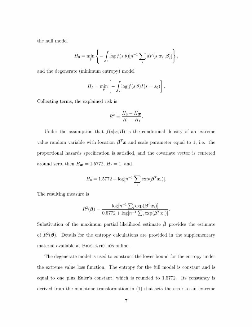
the null model
H0 = minθ
{−∫s
log f(s|θ)[n−1∑i
dF (s|xi;β)]
},
and the degenerate (minimum entropy) model
HI = minθ
[−∫s
log f(s|θ)I(s = s0)
].
Collecting terms, the explained risk is
R2 =H0 −HxH0 −HI
.
Under the assumption that f(s|x;β) is the conditional density of an extreme
value random variable with location βTx and scale parameter equal to 1, i.e. the
proportional hazards specification is satisfied, and the covariate vector is centered
around zero, then Hx = 1.5772, HI = 1, and
H0 = 1.5772 + log[n−1∑i
exp(βTxi)].
The resulting measure is
R2(β) =log[n−1
∑i exp(βTxi)]
0.5772 + log[n−1∑
i exp(βTxi)].
Substitution of the maximum partial likelihood estimate β provides the estimate
of R2(β). Details for the entropy calculations are provided in the supplementary
material available at Biostatistics online.
The degenerate model is used to construct the lower bound for the entropy under
the extreme value loss function. The entropy for the full model is constant and is
equal to one plus Euler’s constant, which is rounded to 1.5772. Its constancy is
derived from the monotone transformation in (1) that sets the error to an extreme
7
value random variable with mean zero and scale parameter equal to one. The null
model entropy is the explained risk lost due to ignoring the covariates.
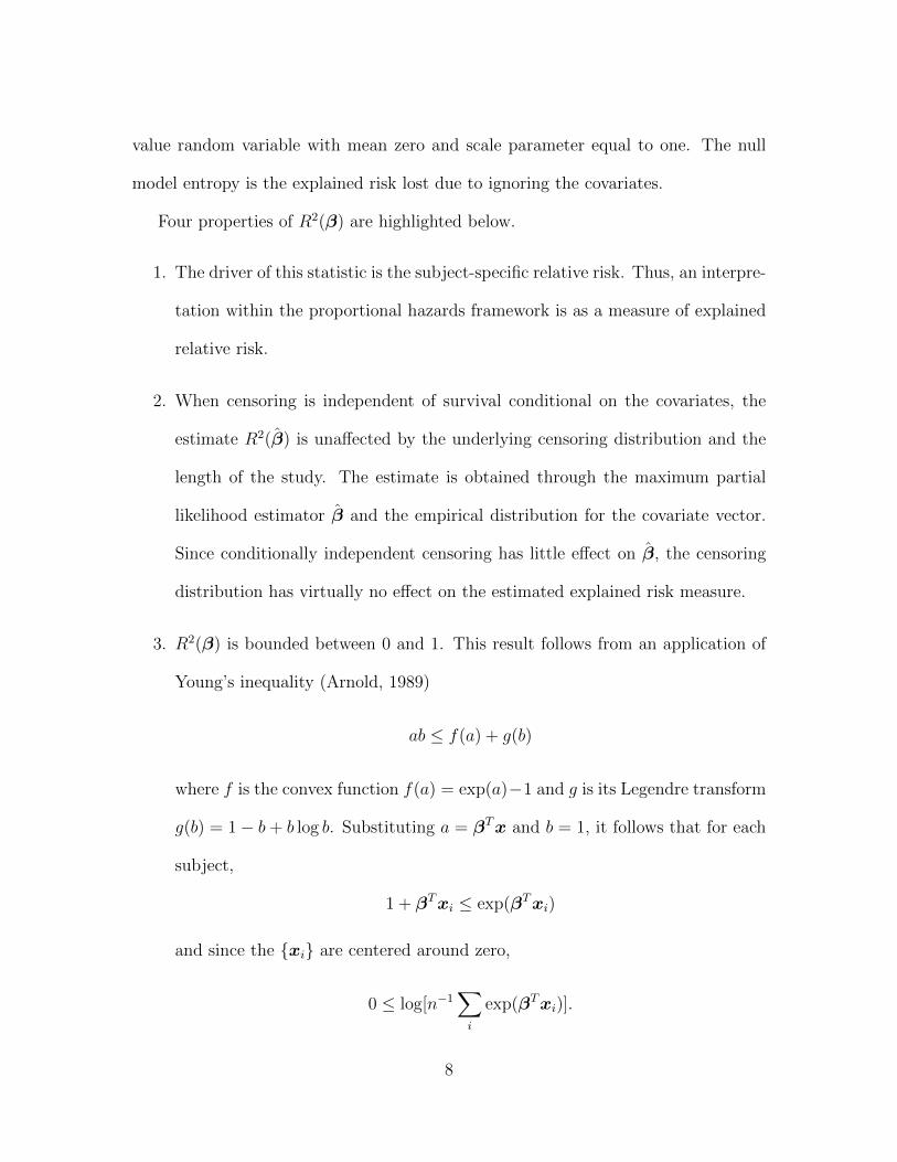
Four properties of R2(β) are highlighted below.
1. The driver of this statistic is the subject-specific relative risk. Thus, an interpre-
tation within the proportional hazards framework is as a measure of explained
relative risk.
2. When censoring is independent of survival conditional on the covariates, the
estimate R2(β) is unaffected by the underlying censoring distribution and the
length of the study. The estimate is obtained through the maximum partial
likelihood estimator β and the empirical distribution for the covariate vector.
Since conditionally independent censoring has little effect on β, the censoring
distribution has virtually no effect on the estimated explained risk measure.
3. R2(β) is bounded between 0 and 1. This result follows from an application of
Young’s inequality (Arnold, 1989)
ab ≤ f(a) + g(b)
where f is the convex function f(a) = exp(a)−1 and g is its Legendre transform
g(b) = 1− b+ b log b. Substituting a = βTx and b = 1, it follows that for each
subject,
1 + βTxi ≤ exp(βTxi)
and since the {xi} are centered around zero,
0 ≤ log[n−1∑i
exp(βTxi)].
8

4. A device that is often cited to assess the adequacy of a newly developed R2
measure is its comparability to the coefficient of determination in the normal
linear model. When R2 is applied to the normal linear scale transformation
model
m(T ) = βTxi + εi,
where m is an unknown monotone function and {εi} are independent, identically
distributed, normal random variables with mean 0 and variance σ2, then
Hx = 12
log(2πσ2e), HI = 12
log(2πσ2), and
H0 =1
2log(2πσ2e) +
1
2n
∑i
[βTxi − n−1
∑j(β
Txj)
σ
]2.
This produces the measure
R2(β) =n−1
∑i
[βTxi − n−1
∑j(β
Txj)]2
σ2 + n−1∑
i
[βTxi − n−1
∑j(β
Txj)]2 ,
which for large n approximates the population value of the coefficient of deter-
mination for the normal linear scale transformation model
varx[E(m(T )|x)]
Ex[var(m(T )|x)] + varx[E(m(T )|x)].
Thus, the proposed statistic is based on a primary component of the proportional
hazards model, the relative risk function. It ranges between zero and one, permit-
ting a standard metric for interpretability, and since it is stable in the presence of
conditionally independent censoring, allows for comparability between studies. In
addition, the simplicity of the estimate R2(β) enables a straightforward derivation of
its asymptotic normal distribution, and ultimately, an asymptotic confidence interval
for its population value ρ2(β) = limn→∞E[R2(β)].
9

Theorem: Assume the {xi} are generated independent and identically distributed
with E(xT1 x1) <∞ and µx(β) = E[exp(βTx1)] > 0. Then
n1/2[R2(β)− ρ2(β0)] converges in distribution to N [0, D−1(β0)V (β0)D−T (β0)],
where ρ2(β0) =log[µx(β0)]
0.5772 + log[µx(β0)]V (β0) = var(β), D(β0) =
{∂R2(β)
∂β
} ∣∣∣∣β=β0
.
The estimate of the asymptotic variance of R2(β) follows by substituting the max-
imum partial likelihood estimate β for β0 in each component. The derivation of
this asymptotic distribution is provided in the supplementary material available at
Biostatistics online.
4. Contribution of a Subset of Factors to the Explained Risk
In addition to the overall assessment of explained risk, the relative importance of
a subset of factors from the full model may be ascertained. The full proportional
hazards model is denoted by
λ(t|x, z) = λ0(t) exp[βTx+ γTz]
and the density of a subset model, obtained by ignoring the heterogeneity due to the
covariate vector z, is denoted by
fx(z)(t|x) = n−1∑j
f(t|x, zj).
The extreme value entropy loss function is now written as
− log f(s|θx, θz) = −[(s− θx − θz)− exp{(s− θx − θz)}],
where θx = βTx and θz = γTz. The entropy for the full model is Hx,z = 1.5772 and
the entropy for the subset model, ignoring the heterogeneity due to z, is
Hx(z) = n−1∑i
{min
θ=θx+θz
(−∫s
log f(s|θ)[n−1∑j
dF (s|xi, zj;β,γ)]
)}.
10

= 1.5772 + log[n−1∑j
exp(γTzj)].
Therefore, the contribution of the covariate vector z to the explained relative risk
R2x(z) =
Hx(z) −Hx,zH0 −HI
is equal to
R2x(z) =
log[n−1∑
j exp(γTzj)]
0.5772 + log[n−1∑
j exp(βTxj + γTzj)].
Its estimate is obtained through substitution of the partial likelihood estimates (β, γ)
from the full model.
5. Simulations
A simulation study was performed to assess the properties of the explained relative
risk measure and compare the results to the likelihood ratio, Kent and O’Quigley,
and Xu and O’Quigley measures of explained risk described in Section 2.
The survival times were generated from the regression model
Ti = exp[1 + 2Xi + εi]
where the scalar covariate Xi was a standard normal random variable, and the εi were
independent identically distributed Weibull random variables with scale parameter 1
and shape parameter taking on the values {1.20, 0.80, 0.50, 0.30}. These parameters
were chosen to create a wide range for the explained risk measures. The regression
model produces a proportional hazards relationship between the covariate and sur-
vival time. Censoring times were generated independently of the covariate or survival
time, from a uniform distribution with support (0, τ), where τ was varied to produce
average censoring proportions approximately equal to {0, 0.25, 0.50, 0.75}. For each
simulation the sample size was 100 and the average of 5000 replications was reported.
11

To determine the accuracy of these measures, the survival times were log trans-
formed to produce a loglinear model, and the coefficient of determination
R2LLM = 1−
∑i[log ti − β
Txi]
2∑i[log ti − n−1
∑i(log ti)]2
was computed in the uncensored data case, where β represents the least squares
estimate. Under the Korn and Simon (1991) classification, R2LLM is a measure of
explained residual variation, and is expected to be smaller, more pessimistic, than
the explained risk statistics under study (Henderson, 1995). This statistic, which is
common in the uncensored data case, does not account for censoring and hence the
need for alternative measures.
The results in Table 1 indicate that the proposed explained relative risk R2 and the
Kent and O’Quigley measure R2KO are unaffected by the percent censored, whereas
the likelihood ratio R2LR and Xu and O’Quigley measure R2
XO fluctuate as the cen-
soring proportion (maximum follow-up time) varies. In the uncensored data case,
the explained relative risk, the likelihood ratio statistic, and the Xu and O’Quigley
measures were comparable to R2LLM over the range of Weibull shape parameters ex-
plored. The likelihood ratio statistic and the Xu and O’Quigley measures, however,
increased as the percent censoring increases. The Kent and O’Quigley statistic R2KO
had a greater bias than the explained relative risk R2, when compared to R2LLM and
R2LR in the uncensored case. Since it is unaffected by censoring, the bias in R2
KO
remained across censoring rates. These results indicate that the explained relative
risk R2 statistic is both stable and accurate relative to the other commonly cited
measures of explained risk.
The estimated standard error of the proposed R2 is comparable to the simula-
12

tion standard error of the estimate. Its estimated variability (ASE) increased as the
censoring proportion increased and as the Weibull shape parameter decreased. The
latter result stems from the property that under the generated Weibull regression
model, a decrease in the shape parameter indicates an increase in the variability of
the underlying survival times.
Additional simulations (not shown) were generated for survival times from a
proportional hazards model with a baseline cumulative hazard function equal to
Λ0(T ) = log(1 + T ). Thus, the survival times were not generated from a Weibull
distribution, but the data still maintain the proportional hazards structure. The
results were similar to the Weibull simulations in Table 1.
6. Prostate Cancer Data Example
A model was developed on 1006 castrate resistant metastatic prostate cancer patients,
using 10 prognostic factors within a proportional hazards model (Armstrong et al.,
2007). The model produced a concordance index (Harrell et al. 1984), a measure
of model discrimination for the survival time, equal to 0.38 when transformed to a
[0, 1] scale. This result indicates that there remains important unknown or unrecorded
factors that explain the heterogeneity in relative risk. In 2009, a study was undertaken
to explore the role of a new biomarker, circulating tumor cells (CTC), as a prognostic
factor for survival time in this prostate cancer population (Scher et al., 2009). CTC
is a blood-based assay that provides information on the accumulation of tumor cells
in the peripheral blood.
In the 2009 study, a proportional hazards model was generated from a cohort of
one hundred and thirty six patients with castrate resistant metastatic prostate can-
13

cer. In addition to CTC, the factors considered for this model were: hemoglobin,
prostate-specific antigen (PSA), lactate dehydrogenase (LDH), alkaline phosphatase,
and albumin. A logarithmic transformation of some of the factors was used to account
for their positively skewed distribution. The results from this analysis are presented
in Table 2a. The test of the proportional hazards assumption developed by Grambsch
and Therneau (1994) provided no evidence that the proportional hazards assumptions
were violated for the full model (p = 0.681). The factors LDH (p < 0.001) and CTC
(p = 0.004) were the strongest prognostic factors, indicating that CTC adds to un-
derstanding patient risk in the metastatic prostate cancer population. However, the
magnitude of the p-value is sensitive to sample size and it alone is not sufficient to
evaluate a model’s predictive power of risk assessment. To assess the model’s ade-
quacy in explaining relative risk, the evaluation provided in Table 2a is complemented
with the calculation of the proposed R2 statistic in Table 2b.
For the six factors under study, the explained relative risk is R2 = 0.581 (se =
0.086). The R-square value for the other approaches examined in the simulations
were: R2LR = 0.579, R2
KO = 0.540, and R2XO = 0.607. Table 2b indicates the influence
of the covariate subsets in the determination of R2. As expected, the two factors
that individually provide the greatest contribution to explained relative risk are LDH
and CTC. The combination of LDH and CTC generated an R2 = 0.411, indicating
that over two-thirds of the model’s explained relative risk was generated by these two
factors. Adding hemoglobin to these two factors produced anR2 = 0.547, representing
94% of the explained relative risk. The incremental value of the other factors (PSA,
alkaline phosphatase, and albumin) to the explained relative risk was small.
14

7. Discussion
The measure of explained relative risk for the Cox model is appealing due to its
computational simplicity and it is unaffected by censoring that is independent of
survival conditional on the covariates. This stability stems from the proportional
hazards specification and the fact that the relative risk is independent of follow-
up time. The robustness of this measure may also be seen as a drawback, since
the assumption of a constant relative risk with respect to time may be deemed too
restrictive. From the analyst’s standpoint, a prerequisite to its application is that
goodness of fit methods such as Grambsch and Therneau (1994) or Lin et al. (1993)
have been applied and no violations of the model assumptions are found.
Royston (2006) states that the properties of a good explained variation measure
are: 1) approximately independent of the amount of (independent) censoring; 2)
reducing to R2 for the normal linear model; 3) maintaining the nesting property for
a subset of variable, i.e. model1 ⊂ model2 then R21 < R2
2; 4) R2 increases with the
strength of the association; 5) construction of a confidence interval for the measure.
With the exception of property 3, due to the non-nesting of proportional hazards
models, the proposed R2 measure satisfies these conditions.
Historically, patients with a given disease were classified into a small number
of clinically defined stages that defined patient risk. In recent years, a greater un-
derstanding of the disease process has led to an increase in the granularity of risk
assessment. It is, however, unclear whether this increase in model complexity has re-
sulted in a greater accuracy in the determination of patient risk. If these models are
accepted uncritically, it is problematic when they are used in clinical decision making,
for example as selection criteria for entry into a clinical trial or as trial stratification
15

variables. A highly accurate risk model is necessary for its confident application. The
explained relative risk statistic, which measures the reduction in randomness due to
the introduction of patient risk factors, provides a stable measure of accuracy in the
presence of conditionally independent right censored data and is straightforward to
apply.
Supplementary material
Supplementary material is available at http://www.biostatistics.oxfordjournals.org
Acknowledgements
The author thanks an associate editor and the reviewers for comments that improved
the content of this manuscript.
16

References
Armstrong, A. J., Garrett-Mayer, E. S., Yang, Y. C. O., de Wit,
R., Tannock, I. F. and Eisenberger, M. (2007). A contemporary prog-
nostic nomogram for men with hormone-refractory metastatic prostate cancer:
A TAX327 study analysis. Clinical Cancer Research 13, 6396-6403.
Arnold, V. I. (1989). Mathematical Models of Classical Mechanics (second
edition) New York: Springer.
Graf, E., Schmoor, C., Sauerbrei, W. and Schumacher, M. (1999).
Assessment and comparison of prognostic classification schemes for survival
data. Statistics in Medicine 18, 2529-2545.
Grambsch, P. M. and Therneau, T. M. (1994). Proportional hazards tests
and diagnostics based on weighted residuals. Biometrika 81, 515-526.
Harrell, F.E., Lee, K.L., Califf, R.M., Pryor, D.B. and Rosati,
R.A. (1984). Regression modeling strategies for improved prognostic predic-
tion. Statistics in Medicine 3, 143-52.
Heinzl, H. (2000). Using SAS to calculate the Kent and O’Quigley measure of
dependence for Cox proportional hazards regression model. Computer Methods
and Programs in Biomedicine 63, 71-76.
Henderson, R. (1995). Problems and prediction in survival data analysis.
Statistics in Medicine 14, 161-184.
Kent, J. T. (1983). Information gain and a general measure of correlation.
Biometrika 70, 163-173.
17

Kent, J. T. and O’Quigley, J. (1988). Measures of dependence for censored
survival data. Biometrika 75, 525-534.
Korn, E. L. and Simon, R. (1990). Measures of explained variation for survival
data. Statistics in Medicine 9, 487-503.
Korn, E. L. and Simon, R. (1991). Explained residual variation, explained
risk, and goodness of fit. The American Statistician 45, 201-206.
Lin, D. Y., Wei, L. J., Ying, Z. (1993). Checking the Cox model with
cumulative sums of martingale-based residuals. Biometrika 80, 557-572.
O’Quigley, J. and Xu, R. (2001). Explained variation in proportional hazards
regression. Handbook of Statistics in Clinical Oncology. 397-409; Editor: John
Crowley, Marcel Dekker, New York.
Rosthoj, S. and Keiding, N. (2004). Explained variation and predictive accu-
racy in general parametric statistical models: The role of model misspecification.
Lifetime Data Analysis 10, 461-472.
Royston, P. (2006). Explained variation for survival models. The Stata Journal
6, 83-96.
Scher, H. I., Jia, X., de Bono, J. S., Fleisher, M., Pienta, K. J.,
Raghavan, D. and Heller G. (2009). Circulating tumour cells as prognos-
tic markers in progressive, castration-resistant prostate cancer: a reanalysis of
IMMC38 trial data. Lancet Oncology 10, 233-239.
Xu, R. and O’Quigley, J. (1999). A measure of dependence for proportional
hazards models. Journal of Nonparametric Statistics 12, 83-107.
18

Table 1. Simulation results for measures of explained risk based on the propor-
tional hazards model. The columns in the table represent: Shape, variability of the
underlying event times; PRC, percent right censored; R2, the proposed measure of ex-
plained relative risk; R2LR, the likelihood ratio measure; R2
KO, the Kent and O’Quigley
measure; R2XO, the Xu and O’Quigley measure; R2
LLM , the loglinear model coefficient
of determination; ASE, average estimated standard error; SSE, standard deviation of
the simulation estimates.
Shape PRC R2 R2LR R2
KO R2XO R2
LLM ASE SSE
1.20 0.747 0.814 0.913 0.849 0.887 0.033 0.053
1.20 0.496 0.813 0.873 0.849 0.842 0.038 0.045
1.20 0.257 0.815 0.838 0.849 0.810 0.027 0.041
1.20 0.000 0.813 0.796 0.849 0.789 0.776 0.031 0.040
0.80 0.743 0.678 0.793 0.717 0.755 0.120 0.082
0.80 0.512 0.675 0.745 0.715 0.710 0.047 0.069
0.80 0.257 0.676 0.699 0.715 0.672 0.048 0.062
0.80 0.000 0.677 0.652 0.716 0.644 0.610 0.059 0.060
0.50 0.758 0.461 0.560 0.500 0.537 0.115 0.119
0.50 0.507 0.461 0.521 0.501 0.490 0.082 0.093
0.50 0.243 0.458 0.482 0.498 0.460 0.097 0.082
0.50 0.000 0.459 0.444 0.499 0.439 0.383 0.082 0.077
0.30 0.744 0.245 0.297 0.273 0.286 0.118 0.121
0.30 0.517 0.240 0.277 0.268 0.267 0.079 0.094
0.30 0.241 0.243 0.263 0.272 0.254 0.092 0.080
0.30 0.000 0.240 0.240 0.269 0.237 0.188 0.092 0.074
19

Table 2a. Estimated coefficients, standard errors, and p-values from the partial
likelihood.
Factor Coefficient Std Error P-value
Hemoglobin (HGB) -0.150 0.091 0.098
log Prostate-Specific Antigen (PSA) 0.011 0.089 0.901
log Lactate Dehydrogenase (LDH) 1.225 0.280 < 0.001
log Alkaline Phosphatase 0.052 0.185 0.778
Albumin -0.006 0.030 0.838
log Circulating Tumor Cells (CTC) 0.225 0.078 0.004
Table 2b. Contribution of a subset of factors to R2.
Factor Partial R2
Hemoglobin (HGB) 0.022
log Prostate-Specific Antigen (PSA) < 0.001
log Lactate Dehydrogenase (LDH) 0.201
log Alkaline Phosphatase < 0.001
Albumin < 0.001
log Circulating Tumor Cells (CTC) 0.068
log LDH + log CTC 0.411
log LDH + log CTC + HGB 0.547
All factors 0.581
20