the cost of checking proportional hazards bryan e....
TRANSCRIPT

The Cost of Checking Proportional Hazards
Bryan E. ShepherdDepartment of Biostatistics,
Vanderbilt University School of Medicine, Nashville, TN, 37232, USA
SUMMARY
Confidence intervals (CI) and the reported predictive ability of statistical models may bemisleading if one ignores uncertainty in the model selection procedure. When analyzingtime-to-event data using Cox regression, one typically checks the proportional hazards(PH) assumption and subsequently alters the model to address any violations. Such anexamination and correction constitutes a model selection procedure, and if not accountedfor could result in misleading CI. With the bootstrap, I study the impact of checking thePH assumption using (1) data to predict AIDS-free survival among HIV-infected patientsinitiating antiretroviral therapy, and (2) simulated data. In the HIV study, due to non-PH, a Cox model was stratified on age quintiles. Interestingly, bootstrap CI that ignoredthe PH check (always stratified on age quintiles) were wider than those which accountedfor the PH check (on each bootstrap replication tested PH and corrected through strat-ification only if violated). Simulations demonstrated that such a phenomenon is not ananomaly, although on average CI widen when accounting for the PH check. In most simu-lation scenarios, coverage probabilities adjusting and not adjusting for the PH check weresimilar. However, when data were generated under a minor PH violation, 95% bootstrapCI ignoring the PH check had coverage of 0.77 as opposed to 0.95 for CI accounting forthe PH check. The impact of checking the PH assumption is greatest when the p-valueof the test for PH is close to the test’s chosen Type I error probability.
KEYWORDS: survival analysis; Cox regression; bootstrap; prediction; model uncertainty;AIDS.
1

1. INTRODUCTION
Most confidence intervals, P-values, and prediction models reported in medical jour-
nals are based on the assumption that the underlying probability model used for the
analysis is known. For example, a multivariable analysis may estimate the effect of a
treatment on an outcome after adjusting for several other variables. Often, however,
those variables are a subset of many candidate adjustment variables, the shape of the re-
lationship between covariables and the outcome is uncertain, and different distributional
assumptions and transformations are considered. It is well known that if this uncertainty
in the model selection process is ignored, P-values, confidence intervals, and the reported
success of prediction models may be misleading, with researchers claiming to know more
than the information content in the data support [1-6].
By bootstrapping the entire modeling process, valid confidence intervals and mea-
sures of the discriminatory ability of prediction models can be computed [7-9]. Using the
bootstrap, Faraway demonstrated the cost of using the data in order to select a model
[5]. In a linear regression analysis, he considered variable transformations, selected pre-
dictors for the model, checked for outliers, examined overly influential observations, and
investigated hederoscedasticity. He then bootstrapped the entire model fitting process,
programming, for example, a correction for hederoscedasticity if it was seen in a bootstrap
sample. Faraway then demonstrated how non-parameteric bootstrap confidence intervals
widen as each of the different components of the model selection process is accounted for.
Based on the results of Faraway and others, analysts have been encouraged to bootstrap
the entire modeling procedure [10].
When dealing with right censored data, researchers often use Cox regression, which
assumes proportional hazards (PH). There are many suggested methods for testing the va-
lidity of this assumption (e.g., using log(-log) plots, hazard ratio plots, smoothed Schoen-
2
feld residual plots [11], etc.). When the PH assumption is violated, there are various
approaches for changing the model (e.g., stratification, time-dependent covariables, ac-
celerated failure time models, etc.). A highly cited paper recommends bootstrapping the
process of examining and correcting possible violations of the PH assumption (points 10
and 13 of [12]). However, I know of no analysis that has bootstrapped the process of
checking the PH assumption.
The purpose of this paper is to examine the cost of data analysis when checking and
correcting violations of the proportional hazards assumption. In section 2 I will introduce
an observational HIV study from which a model was created to examine predictors of
AIDS-free survival, and I will describe my model fitting procedures. In section 3 I will
obtain confidence intervals and measures of the model’s predictive ability by bootstrapping
the entire model fitting procedure, including checking and adjusting for violations of the
proportional hazards assumption. Following the approach of Faraway, I will compare these
confidence intervals and statistics to similar quantities that do not account for the full
model fitting uncertainty. Due to some unexpected results, in section 4 I will investigate
through simulations the importance of accounting for the PH check under four different
data generating scenarios. In section 5 I will discuss implications of these results on
general data analysis.
2. HIV EPIDEMIOLOGY STUDY
The Collaborations in HIV Outcomes Research United States cohort (CHORUS)
followed HIV positive individuals throughout the United States. A recent study exam-
ined predictors of an AIDS defining event (ADE [13]) or death for individuals initiating
highly-active antiretroviral therapy (HAART). Of particular interest was whether %CD4
at initiation of HAART was a good predictor of ADE/death. Other predictor variables
were absolute CD4 count (aCD4), log10-transformed viral load (VL), age, race (white or
3
non-white), gender, and whether an individual had previously used antiretroviral therapy.
A total of 1891 participants met the inclusion criteria and were followed for a median of 55
weeks (interquartile range, 23 to 83 weeks); 468 individuals had an ADE or died. Details
have been previously published [14].
To evaluate the association between %CD4 at the start of therapy on ADE or death,
I fit a Cox proportional hazards model adjusting for each of the above variables. To
improve numeric stability, %CD4 and aCD4 were square-root transformed. All predictor
variables were included in the analyses without variable selection. An interaction between
%CD4 and aCD4 was also included in the model, because a prior study suggested the
association between %CD4 and disease progression varied according to different levels of
aCD4 [15]. My model fitting procedure was the following:
1. Linearity in the hazard was not necessarily assumed, so continuous predictors
(%CD4, aCD4, VL, and age) were expanded by fitting restricted cubic splines with k
knots (with the knots located at the default levels of R’s Design package [10]). To limit
the number of candidate models, the number of knots, k, was set equal for all continuous
predictors, either 0 (linearity), 3, 4, or 5 knots. The same number of knots were also used
in the interaction term between %CD4 and aCD4; the interaction was specified using the
Design package function %ia% which is referred to as a restricted interaction because it
does not include products involving nonlinear components on both variables. The number
of knots used in the final model, k = 3, was chosen as that which maximized the Akaike
information criteria (AIC).
2. A test for interaction between %CD4 and aCD4 was performed. This was a
likelihood ratio test with 3 degrees of freedom (d.f.) because it included both linear
(1 d.f.) and nonlinear (2 d.f.) terms. The test was found significant at the 0.05-level
(p = 0.004), so the interaction was left in the model.
4

3. The proportional hazards assumption was tested using an approach outlined else-
where [11,12]. In short, scaled Schoenfeld residuals were computed separately for each
predictor and the proportional hazards assumption was tested using a “correlation with
time” test, using the R function cox.zph in the survival package. There was data evi-
dence of a possible violation to the proportional hazards assumption (p = 0.038). The
variable deemed most likely to contribute to the non-proportionality, age, was adjusted
for using stratification (allowing the form of the baseline hazard to vary across levels of
age). Strata were created based on age quintiles. Age was left in the linear predictor
(with 3 knots) to capture any residual information.
When not accounting for the model fitting procedures, %CD4 was found to be a
significant predictor of the time until ADE/death (p = 0.002) for individuals initiating
HAART. Controlling for all other variables and adjusting for aCD4 at its median value of
240 (due to an interaction), the estimated hazard ratio for an individual with %CD4=24
(third quartile) versus %CD4=9 (first quartile) was 0.58 (95% confidence interval (CI)
of 0.41-0.82). The predicted 5-year ADE-free survival, adjusting for all variables at their
medians, was 0.77 (95% CI, 0.72-0.81). Discrimination was measured using Harrell’s
c-statistic [12], defined as the proportion of patient pairs in which predictions and out-
comes were concordant. (Considering the strata in the final model, the c-statistic was
computed using predicted ADE-free survival at time 5 years). The apparent estimate of
discrimination was 0.676.
3. EXAMINING THE COST OF THE MODEL FITTING PROCEDURE
3.1. Bootstrapping the Model Fitting Procedure
Using the bootstrap, I next examined the change in confidence intervals and c-statistic
when accounting for varying degrees of the model fitting uncertainty. In each of 1000
5

bootstrap replications I fit a new model to the bootstrapped data using the same 3 model
fitting steps described in Section 2. Specifically,
1. The number of knots, k, (0, 3, 4, or 5; the same number for all continuous variables)
was chosen as the value that maximized the AIC.
2. A test for interaction between %CD4 and aCD4 (including both linear and non-
linear terms, if any were selected in step 1) was performed and the interaction was left in
the model if found significant at the 0.05-level.
3. As described above, proportional hazards was tested. In the event of violation
(p < 0.05), I stratified over the variable which contributed most to this violation. If this
variable happened to be a continuous predictor, then strata were created based on quintiles
of the continuous variable, with the continuous variable (with the chosen number of knots)
remaining in the model’s linear predictor. If the stratification variable was discrete, it
did not remain in the linear predictor. The variable of primary interest, %CD4, was not
permitted as a choice for stratification, nor was the interaction between %CD4 and aCD4.
If either %CD4 or the interaction was chosen as the most likely violator of proportional
hazards, stratification was instead performed over the next most likely variable.
Taking these steps together, there were 4× 2× 7 = 56 possible model forms based on
4 different possible numbers of knots, an interaction (or not), and stratifying (or not) over
any of 6 variables. This bootstrap procedure accounts for full model fitting uncertainty.
Similar to Faraway [5], I also obtained estimates bootstrapping all or part of the model
fitting procedure. Using the same bootstrapped data, I obtained estimates by fitting
a model: A) ignoring all model fitting uncertainties by using none of the above steps
(assuming k = 3 knots, an interaction, and stratifying by age quintiles), B) accounting
for uncertainty with regards to the number of knots by using step 1 only (assuming an
6
interaction and stratifying by age quintiles), C) accounting for uncertainty with regards
to the number of knots and whether there was an interaction by using steps 1 and 2 only
(stratifying by age quintiles), and D) accounting for full model uncertainty by using steps
1, 2, and 3.
3.2. Results
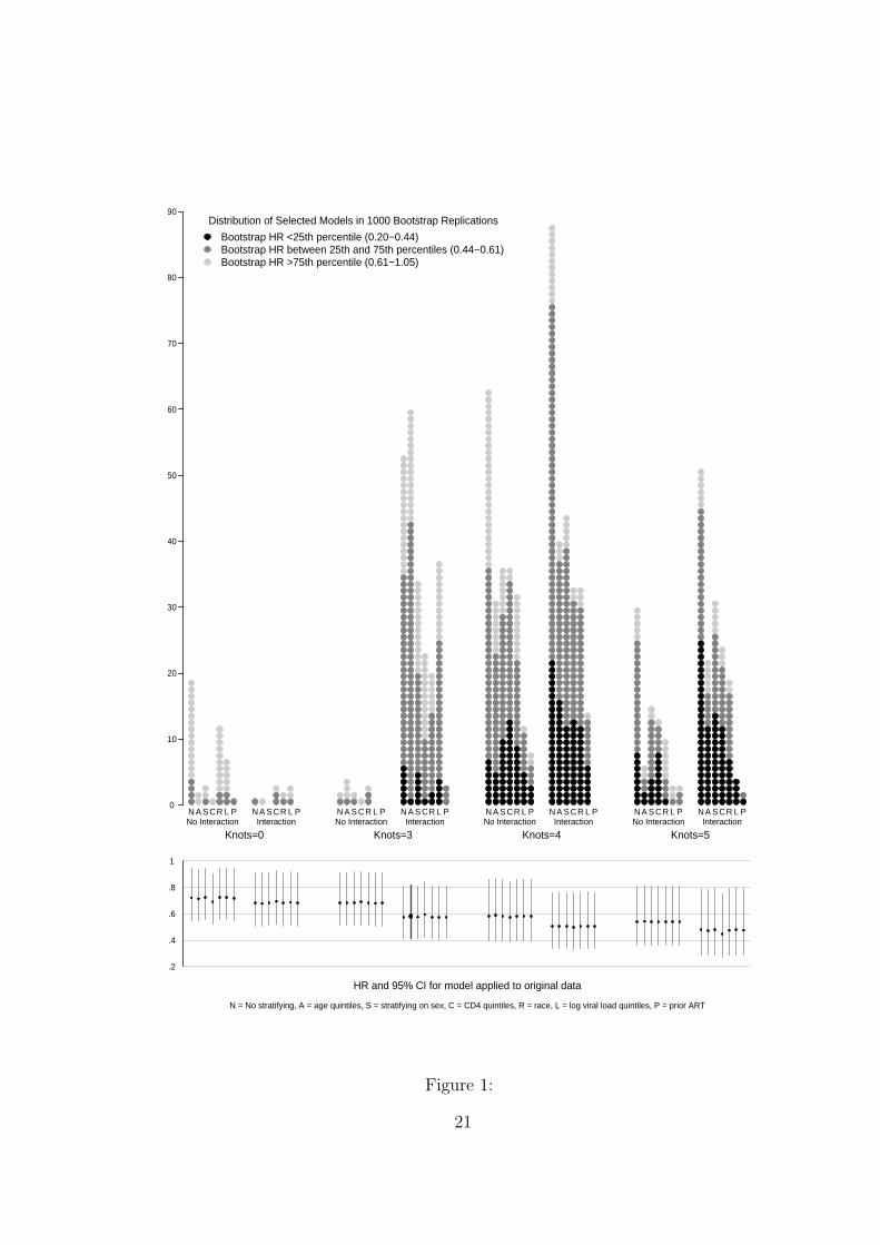
When accounting for full model uncertainty, bootstrap replications substantially var-
ied in the number of knots selected, the presence of an interaction, and if stratification
was necessary what variable was stratified. Of the 1000 bootstrap replications, 55 selected
no knots, 242 selected 3 knots, 470 selected 4 knots, and 233 selected 5 knots; 355 selected
no interaction, 645 selected an interaction; 307 selected no stratification, 166 stratified
by age, 165 stratified by sex, 134 stratified by aCD4, 131 by race, 80 by VL, and 17 by
prior ART. Figure 1 shows the distribution across all 56 possible model choice levels with
shading according to quartiles of the bootstrap hazard ratios of %CD4 on time to AIDS
or death. The most common model (selected by 88 bootstrap replicates) was 4 knots, an
interaction, and no stratifying necessary. The second most common model (selected by
63 bootstrap replicates) was 4 knots, no interaction, and no stratifying. The third most
common model (selected by 61 bootstrap replicates) was the model used in the actual
analysis, 3 knots, an interaction, and stratifying by age quintiles. The bottom of Figure 1
contains the estimated hazard ratio and 95% CI (based on asymptotic variance) for each
of the 56 models applied to the original data.
Figure 2 contains a plot of the 2.5th and 97.5th percentiles of the bootstrap distri-
bution of the estimated hazard ratios as a function of the amount of model uncertainty
accounted for in the bootstrap procedure, corresponding to non-parametric percentile
bootstrap 95% confidence intervals. The width of the 95% confidence intervals increased
when accounting for uncertainty in selecting the number of knots. The median boot-
7

strapped hazard ratio also decreased. Afterwards, the model uncertainty and the median
hazard ratio stayed about the same, regardless of whether I accounted for model uncer-
tainty regarding inclusion of the interaction or strata to meet the proportional hazards
assumption. The second plot in Figure 2 is similar, looking at the predicted 5 year ADE-
free survival as a function of model uncertainty accounted for in the bootstrap procedure.
In this case, 95% confidence intervals actually decreased if I accounted for the uncertainty
in the proportional hazards assumption.
The estimated c-statistic computed earlier, 0.676, is an over-estimate of how well
this model will perform in independent data. Based on the bootstrap accounting for no
modeling uncertainty, the estimated optimism [8] of the c-statistic is 0.062; accounting
for uncertainty in the number of knots, 0.073; accounting for uncertainty in the number
of knots and the interaction 0.073; and accounting for full model uncertainty (knots, in-
teraction, and proportional hazards), the optimism is 0.052. That means that applied to
independent data, one would expect the c-statistic to be 0.676− 0.052 = 0.624. Interest-
ingly, the c-statistic is higher when accounting for the full model fitting uncertainty than
when ignoring the PH check.
Using the bootstrap, one can also obtain estimates for the amount of over-fitting
or shrinkage when applying this model to independent data; a shrinkage estimate of 1
indicates no overfitting ([10] page 95). The estimates of shrinkage if one accounts for no
modeling uncertainty, knots, knots and interaction, or full are 0.70, 0.66, 0.67, and 0.62,
respectively.
It should be noted that of the 693 bootstrap replications where the proportional
hazards assumption was violated, 486 still violated the proportional hazards assumption
after stratifying as described above.
8

To summarize, I found it surprising and noteworthy that 51 of the possible 56 models
were selected at least once in 1000 bootstrap replications, and that the width of confidence
intervals and the estimated optimism of the c-statistic actually decreased when accounting
for checking and fixing violations of the proportional hazards assumption. Each of these
statistics was re-computed a second time using 1000 new bootstrap replications with
similar results (data not shown).
4. SIMULATIONS
4.1 Simulation Setup
I further explored the properties of adjusting for the proportional hazards check
through simulation. Data were generated under four distinct scenarios: A) under a pro-
portional hazards model, B) under a stratified proportional hazards model where the
hazards were slightly unproportional without stratification, C) under a stratified propor-
tional hazards model where the hazards were highly unproportional without stratification,
and D) under a nonproportional hazards model.
In each simulation, for i = 1, · · · , N(N = 2000), the length of time followed, yi, and
the event indicator di, were computed in the following manner:
1. Xi = (X1i, X2i, X3i, X4i) = (Zi, X4i) were generated with Zi ∼ N(a, b) and X4i ∼Bernoulli((1 + exp(−cZi))
−1) where a = (3.9, 15, 38.8), b was a symmetric matrix with
diagonal (1.8, 43, 65) and off-diagonal (b12 = 7.5, b13 = −0.8, b23 = −1.3), and c =
(−0.49,−0.14, 0.0016, 0.029). These choices were motivated by the observed distribu-
tion of the covariates square root %CD4, square root aCD4, age, and prior antiretroviral
therapy in the CHORUS dataset.
2. The length of followup, Yi = min(Ti, Ci), and the event indicator, δi = I(Yi = Ti),
were generated, where Ci/120 ∼ Beta(1.3, 1) and Ti was generated as follows:
9

A) Ti = (−log(Ui)/(λexp(βXi))1/ν , with Ui ∼ Uniform(0, 1), β = (−0.18,−0.04, 0.006, 0.53),
ν = 0.693, and λ = 0.031. This model was based on the best fitting Weibull distribution
to the CHORUS data [16].
B) Same as A, except ν = 0.5, λ = 0.1 if X3i < 32 (the lowest age quintile) and
ν = 0.73, λ = 0.025 if X3i ≥ 32. This generates data where the proportional hazards
assumption is slightly violated without stratification.
C) Same as A, except ν = 2.2, λ = 0.0001 if X3i < 32 and ν = 0.5, λ = 0.065
if X3i ≥ 32. This generates data where the proportional hazards assumption is highly
violated without stratification.
D) Ti = exp(Ui), with Ui ∼ N(µi, σ2) where µi = 4.30 + 0.33X1i + 0.064X2i −
0.006X3i − 0.689X4i and σ = 2.47. This model was based on the best fitting lognormal
distribution to the CHORUS data.
In each simulation a Cox proportional hazards model was initially fit to the data.
Next, the proportional hazards assumption was tested. If the proportional hazards as-
sumption was violated at the 0.05 level, then a new Cox proportional hazards model was
fit to the data, stratifying by the covariate deemed to most contribute to the nonpropor-
tionality (quintiles/levels for continuous/discrete covariates, respectively, as described in
section 3.1). The relationship between continuous predictors and the hazard was assumed
to be linear without any interactions. Therefore, the only model fitting procedure was
the check and the possible correction of proportional hazards.
For each simulated dataset, 200 bootstrap replications were performed; in each repli-
cation I both did and did not account for the proportional hazards test/correction. A
total of 500 simulations (each with 200 bootstrap replications) were performed for each
of the four data generation scenarios.
10

4.2 Simulation Results
Simulation results under each of the set-ups described above are summarized in Table
1. The coverage probability and width of the 95% confidence intervals for the hazard ratio
were approximately the same whether or not one accounted for the proportional hazards
check in the bootstrap procedure. This could be expected since for all three PH data
generating scenarios the hazard ratio was the same, whether or not one had to stratify to
meet the PH assumption. It is not surprising that coverage probabilities for the hazard
ratio fitting a PH model to non-PH data (generated under a lognormal distribution) do
not cover at their nominal level. The estimated c-statistic and the estimated shrinkage
were also similar, whether or not one included the PH check in the bootstrap simulation.
In contrast, when accounting for the PH check in 3 of the 4 scenarios the mean width
of confidence intervals for the predicted 5-year survival was wider. The shorter width
of confidence intervals ignoring the PH check resulted in lower coverage probabilities for
the estimated 5-year survival. The coverage probability not accounting for the PH check
was particularly poor when data were generated under the minor PH violation, with 95%
confidence intervals covering only 77% of the time. These results are consistent with
observations made by Altman and Andersen who saw that bootstrap confidence intervals
of predicted survival were much wider when bootstrapping the stepwise regression model
selection process than when assuming the variables included in the model were fixed and
known [3].
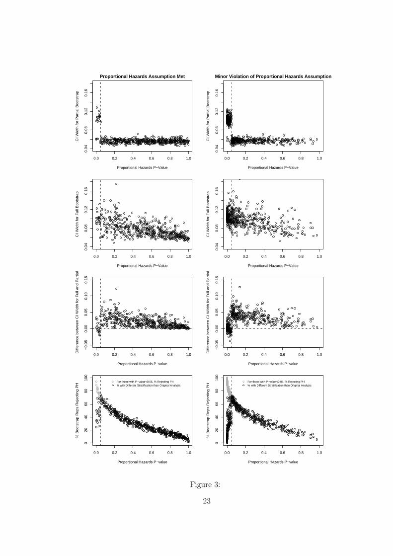
Figure 3 explains why coverage probabilities for the predicted 5-year survival were
especially poor for simulations under the minor violation of PH (right column) compared
to simulations under PH (left column). First, it should be recognized that confidence
intervals for the predicted survival are wider when one stratifies than when one does not
stratify, because stratification requires estimating a separate baseline hazard for each stra-
11

tum. In the simulations, if the PH p-value was > 0.05 then the original model stratified,
the bootstrap replications that ignored the PH check did not stratify, and therefore CI
were narrow; if the PH p-value was < 0.05 then the original model did not stratify, the
bootstrap replications that ignored the PH check always stratified, and therefore CI were
wide (first row of Figure 3). In contrast, if one accounted for the PH check in the boot-
strap replications then the width of confidence intervals was a more continuous function
of the PH p-value. The larger the PH p-value, the less frequently PH was rejected in
the bootstrap replications (bottom row of Figure 3), and therefore the more narrow the
resulting confidence intervals that accounted for the PH check (second row of Figure 3).
Hence, relative to the full bootstrap CI, the partial bootstrap CI were about the same
for p-values under 0.05, and generally too narrow for p-values above 0.05, but especially
narrow for p-values just over 0.05 (third row of Figure 3).
When data were simulated under PH, the distribution of PH p-values, as predicted
by theory, was uniform (left column of Figure 3). In contrast, when data were simulated
under a minor violation of PH, the PH p-value distribution was skewed (right column of
Figure 3), with a large proportion of these p-values just greater than 0.05, in the range
where the difference between the widths of full and partial bootstrap CI was particularly
large. This skewed p-value distribution, and hence the large proportion of simulations
with partial CI that were much too narrow, resulted in especially poor coverage for partial
bootstrap CI simulated under a minor violation of PH.
Confidence intervals were identical both accounting for and not accounting for the
PH check in the simulations with data generated under a major violation of PH. This is
because PH was always rejected with extremely small p-values, and therefore stratifica-
tion in almost all (> 99.9%) bootstrap replications occurred over the correct stratifying
variable, which was the same stratifying variable assumed in the bootstrap replications
12

that ignored the PH check.
Even though confidence intervals widen on average when accounting for the PH check,
this may not be the case in a particular analysis. For example, for the simulations gen-
erated under the minor violation of PH, the mean confidence interval width for survival
ignoring the PH check was 0.073 compared to 0.098 when accounting for the PH check.
However, 78 (16%) of the simulations resulted in shorter confidence intervals when ac-
counting for the PH check than when ignoring it. And of those simulations with a PH
p-value < 0.05, 78/175 (45%) had shorter CI after accounting for the PH check. The
explanation for this phenomenon is also in Figure 3: When the PH p-value was below
0.05, partial bootstrap CI were wide because stratification was assumed for each boot-
strap replication. In contrast, when the p-value was just below 0.05, in some bootstrap
replications the test for PH was not rejected, resulting in no stratification, and therefore
full bootstrap CI which were more narrow than the corresponding partial bootstrap CI.
A close look at the third row of plots in Figure 3 shows that full bootstrap CI widths mi-
nus partial bootstrap CI widths tended to decrease (become negative) as the PH p-value
approached 0.05 from below. Recall that in the HIV example, the PH p-value was 0.038.
Hence, the shorter confidence intervals seen when accounting for the PH check in the HIV
analysis are not anomalies.
Similarly, when accounting for full model fitting uncertainty the estimated optimism
of the c-statistic often decreased, which was also seen in the HIV example. Although
the estimated c-statistic optimism seen in the simulations tended to be slightly less when
ignoring the PH check than when accounting for it, I often saw the opposite in individual
simulations. For example, 165 (33%) of simulations generated under the minor PH viola-
tion had a smaller estimate of optimism when accounting for full model uncertainty than
when ignoring the PH check.
13
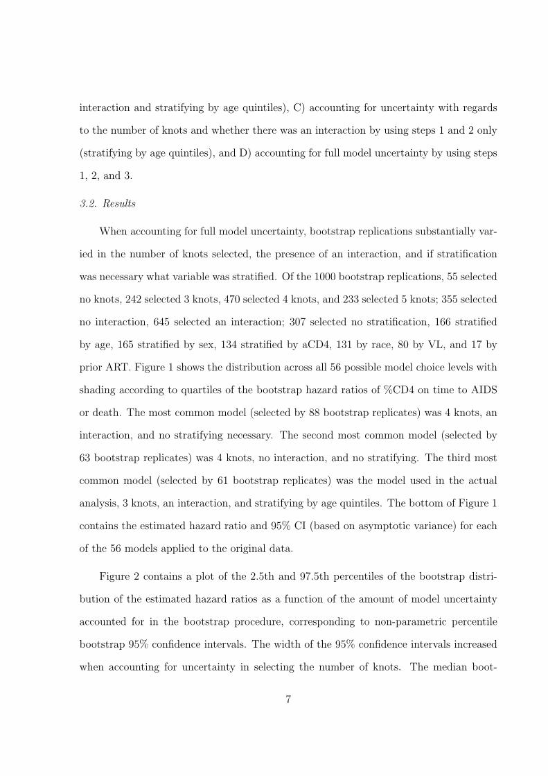
5. DISCUSSION
In this paper I have examined the cost of checking and correcting violations of the
proportional hazards assumption. Similar to others [3,5], I saw that confidence intervals
generally (although not necessarily) widen when one accounts for an increasing amount
of model fitting uncertainty using the bootstrap.
In the simulations, coverage probabilities of 95% CI constructed ignoring the PH check
were as low as 0.77. Although far from exhaustive, the simulations were informative as
to when naive confidence intervals will be especially poor. The PH test p-value is a good
predictor of how many times PH will be rejected in bootstrap simulations. If the PH
p-value is large or very small, then accounting for the PH check in the bootstrap probably
will not have a substantial influence on final results because most models selected in
bootstrap replications will be similar to the model selected in the original data. Ignoring
the PH check appears to be most problematic when the PH p-value is slightly above the
selected Type I error probability for the PH test (0.05 in our case).
In the HIV analysis, CI actually narrowed when accounting for the PH check. In
general, CI that account for model-fitting uncertainty may narrow when the model chosen
for the original data is more complex and results in a more variable estimate compared to
the model not chosen, and when the model selection decision is based on a test which is
likely to result in choosing the less complex model in a substantial percentage of bootstrap
replications. This was the case in the HIV data analysis: In the original analysis I chose
to stratify (selected a more complex model) because of data-evidence suggesting PH was
violated at the 0.05-level (p=0.038); however, in many bootstrap replications stratification
was not selected (resulting in a less complex model) because the p-value for the test for
PH on the bootstrapped data was > 0.05.
14

To simplify and to be able to simulate, I only considered an automated check of PH
using scaled Schoenfeld residuals, and I only corrected for violations of PH through strat-
ification. Of course, there are many alternative ways to investigate the PH assumption
and there are many different approaches to correct violations of PH; results may differ
using alternative approaches. A fair question is the following: What would I have done in
the HIV analysis if, contrary to fact, PH had still been violated even after stratification?
As the model selection process programmed into the bootstrap procedure, which ignored
any further violation of PH, was probably more simple than what I would have actually
done had PH still been violated, my confidence intervals could be affected, particularly
since nearly half of my bootstrap replications in the HIV analysis resulted in a violation of
PH even after stratification. It is nearly impossible, however, to include in the bootstrap
routine solutions for all possible counterfactual scenarios.
Do we need to bootstrap the proportional hazards check and potential correction
procedure every time we test this assumption in routine data analysis? Yes, or we should
use some other approach to account for model fitting uncertainty (e.g., model averag-
ing [17]). Does that mean it will happen in practice? Probably not. The importance
of accounting for model selection uncertainty has been known for years, yet largely ig-
nored. As bootstrapping the check and correction of the PH assumption is quite tedious,
someone could alternatively (and erroneously) conclude that it is best to simply avoid
checking the PH assumption altogether. This would allow the analyst to avoid one prob-
lem, but possibly create a bigger problem – poorly fitting models. In order to facilitate
bootstrapping the PH check/correction, I have placed general R code at the website
http://biostat.mc.vanderbilt.edu/BootstrapProportionalHazards.
ACKNOWLEDGEMENTS
I would like to thank Frank Harrell Jr., Rafe Donahue, and Chun Li for insightful
15

advice, Peggy Schuyler for editing an earlier version of this manuscript, Jeremy Stephens
for programming advice, and the Vanderbilt HIV Epi Outcomes Group for helpful discus-
sions. This work was funded in part by the Vanderbilt-Meharry Center for AIDS Research
(NIH program P30 AI 54999).
REFERENCES
1. Bickel P, Doksum K. An analysis of transformations revisited. Journal of the American
Statistical Association 1981; 76: 296–311.
2. Copas JB. Regression, prediction and shrinkage. Journal of the Royal Statistical
Society, Series B 1983; 45: 311–354.
3. Altman DG, Andersen PK. Bootstrap investigation of the stability of a Cox regression
model. Statistics in Medicine 1989; 8: 771–783.
4. Grambsch PM, O’Brien PC. The effects of transformations and preliminary tests for
non-linearity in regression. Statisticis in Medicine 1991; 10: 697–709.
5. Faraway JJ. On the cost of data analysis. Journal of Compuatational and Graphical
Statistics 1992; 1:213–229.
6. Chatfield C. Model uncertainty, data mining and statistical inference. Journal of the
Royal Statistical Society, Series A 1995; 158: 419–466.
7. Freedman D. Bootstrapping regression models. The Annals of Statistics 1981; 9:1219–
1228.
8. Efron B. Estimating the error rate of a prediction rule: improvement on cross-
validation. Journal of the American Statistical Association 1983; 78: 316–331.
16

9. Efron B, Tibshirani R. An Introduction to the Bootstrap. Chapman and Hall. New
York. 1993.
10. Harrell FE. Regression modeling strategies, with applications to linear models, logistic
regression, and survival analysis. Springer-Verlag. New York. 2001.
11. Grambsch P, Therneau T. Proportional hazards tests and diagnostics based on
weighted residuals. Biometrika 1994; 81: 515–526.
12. Harrell FE, Lee KL, Mark DB. Multivariable prognostic models: issues in developing
models, evaluating assumptions and adequacy, and measuring and reducing errors.
Statistics in Medicine 1996; 15: 361–387.
13. Centers for Disease Control. 1993 Revised classification system for HIV infection
and expanded surveillance case definition for AIDS among adolescents and adults.
MMWR Recomm Rep 1992; 41 (RR–17):1–19.
14. Hulgan T, Shepherd BE, Raffanti SP, Fusco JS, Beckerman R, Barkanic G, Ster-
ling TR. Absolute and percentage CD4+ lymphocytes are independent predictors of
disease progression in HIV-infected persons initiating HAART. Journal of Infectious
Diseases 2007; 195: 425–431.
15. Hulgan T, Raffanti S, Kheshti A, Blackwell RB, Rebeiro PF, Barkanic G, Ritz B,
Sterling TR. CD4 lymphocyte percentage predicts disease progression in HIV-infected
patients initiating highly active antiretroviral therapy with CD4 lymphocyte counts
> 350 lymphocytes/mm3. Journal of Infectious Diseases 2005; 192: 950–957.
16. Bender R, Augustin T, Blettner M. Generating survival times to simulate Cox pro-
portional hazards models. Statistics in Medicine 2005; 24: 1713–1723.
17

17. Draper, D. Assessment and propagation of model uncertainty. Journal of the Royal
Statistical Society, Series B 1995; 57: 45–97.
18
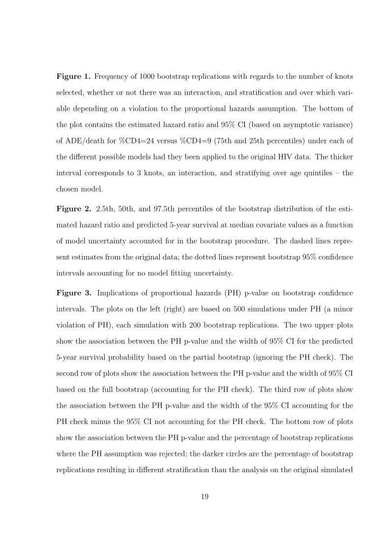
Figure 1. Frequency of 1000 bootstrap replications with regards to the number of knots
selected, whether or not there was an interaction, and stratification and over which vari-
able depending on a violation to the proportional hazards assumption. The bottom of
the plot contains the estimated hazard ratio and 95% CI (based on asymptotic variance)
of ADE/death for %CD4=24 versus %CD4=9 (75th and 25th percentiles) under each of
the different possible models had they been applied to the original HIV data. The thicker
interval corresponds to 3 knots, an interaction, and stratifying over age quintiles – the
chosen model.
Figure 2. 2.5th, 50th, and 97.5th percentiles of the bootstrap distribution of the esti-
mated hazard ratio and predicted 5-year survival at median covariate values as a function
of model uncertainty accounted for in the bootstrap procedure. The dashed lines repre-
sent estimates from the original data; the dotted lines represent bootstrap 95% confidence
intervals accounting for no model fitting uncertainty.
Figure 3. Implications of proportional hazards (PH) p-value on bootstrap confidence
intervals. The plots on the left (right) are based on 500 simulations under PH (a minor
violation of PH), each simulation with 200 bootstrap replications. The two upper plots
show the association between the PH p-value and the width of 95% CI for the predicted
5-year survival probability based on the partial bootstrap (ignoring the PH check). The
second row of plots show the association between the PH p-value and the width of 95% CI
based on the full bootstrap (accounting for the PH check). The third row of plots show
the association between the PH p-value and the width of the 95% CI accounting for the
PH check minus the 95% CI not accounting for the PH check. The bottom row of plots
show the association between the PH p-value and the percentage of bootstrap replications
where the PH assumption was rejected; the darker circles are the percentage of bootstrap
replications resulting in different stratification than the analysis on the original simulated
19

data. The vertical dashed line is at p-value=0.05.
20
N A S CR L P N A S CR L P N A S CR L P N A S CR L P N A S CR L P N A S CR L P N A S CR L P N A S CR L PNo Interaction Interaction No Interaction Interaction No Interaction Interaction No Interaction Interaction
Knots=0 Knots=3 Knots=4 Knots=5
0
10
20
30
40
50
60
70
80
90
.2
.4
.6
.8
1
HR and 95% CI for model applied to original data
N = No stratifying, A = age quintiles, S = stratifying on sex, C = CD4 quintiles, R = race, L = log viral load quintiles, P = prior ART
Distribution of Selected Models in 1000 Bootstrap Replications
Bootstrap HR <25th percentile (0.20−0.44)Bootstrap HR between 25th and 75th percentiles (0.44−0.61)Bootstrap HR >75th percentile (0.61−1.05)
Figure 1:
21

0.3 0.4 0.5 0.6 0.7 0.8
Hazard Ratio
None
Knots
Knots + Interaction
All
0.65 0.70 0.75 0.80
5−Year ADE−Free Survival
None
Knots
Knots + Interaction
All
Figure 2:
22
0.0 0.2 0.4 0.6 0.8 1.0
0.0
40
.08
0.1
20
.16
Proportional Hazards P−Value
CI
Wid
th f
or
Pa
rtia
l Bo
ots
tra
pProportional Hazards Assumption Met
0.0 0.2 0.4 0.6 0.8 1.0
0.0
40
.08
0.1
20
.16
Proportional Hazards P−Value
CI
Wid
th f
or
Pa
rtia
l Bo
ots
tra
p
Minor Violation of Proportional Hazards Assumption
0.0 0.2 0.4 0.6 0.8 1.0
0.0
40
.08
0.1
20
.16
Proportional Hazards P−Value
CI
Wid
th f
or
Fu
ll B
oo
tstr
ap
0.0 0.2 0.4 0.6 0.8 1.0
0.0
40
.08
0.1
20
.16
Proportional Hazards P−Value
CI
Wid
th f
or
Fu
ll B
oo
tstr
ap
0.0 0.2 0.4 0.6 0.8 1.0
−0
.05
0.0
00
.05
0.1
00
.15
Proportional Hazards P−value
Diff
ere
nce
be
twe
en
CI
Wid
th f
or
Fu
ll a
nd
Pa
rtia
l
0.0 0.2 0.4 0.6 0.8 1.0
−0
.05
0.0
00
.05
0.1
00
.15
Proportional Hazards P−value
Diff
ere
nce
be
twe
en
CI
Wid
th f
or
Fu
ll a
nd
Pa
rtia
l
0.0 0.2 0.4 0.6 0.8 1.0
02
04
06
08
01
00
Proportional Hazards P−value
% B
oo
tstr
ap
Re
ps
Re
ject
ing
PH
For those with P−value<0.05, % Rejecting PH% with Different Stratification than Original Analysis
0.0 0.2 0.4 0.6 0.8 1.0
02
04
06
08
01
00
Proportional Hazards P−value
% B
oo
tstr
ap
Re
ps
Re
ject
ing
PH
For those with P−value<0.05, % Rejecting PH% with Different Stratification than Original Analysis
Figure 3:
23

Tab
le1:
Sim
ula
tion
Res
ult
s
Pro
port
ion
PH
Rej
ecte
dH
azar
dR
atio
95%
CI
Pre
dict
edSu
rviv
al95
%C
IE
stim
ated
Est
imat
ed
Aft
erC
over
age
Mea
nC
over
age
Mea
nc-
Stat
isti
cb
Shri
nkag
e
Init
ial
Stra
tific
atio
nP
roba
bilit
yaW
idth
Pro
babi
lity
Wid
thM
ean
(IQ
R)c
Mea
n(I
QR
)
PH
0.04
40.
012
Full
Boo
tstr
ap0.
944
0.34
60.
962
0.07
80.
648
(.64
,.6
6)0.
981
(.98
,.9
9)
Par
tial
Boo
tstr
ap0.
942
0.34
50.
934
0.05
80.
651
(.64
,.6
6)0.
980
(.97
,.9
9)
Min
orV
iola
tion
ofP
H0.
350
0.02
4
Full
Boo
tstr
ap0.
952
0.33
90.
954
0.09
80.
638
(.63
,.6
5)0.
980
(.97
,.9
8)
Par
tial
Boo
tstr
ap0.
954
0.33
90.
768
0.07
30.
643
(.63
,.6
5)0.
965
(.95
,.9
8)
Maj
orV
iola
tion
ofP
H1.
000
0.05
2
Full
Boo
tstr
ap0.
938
0.32
80.
952
0.10
20.
630
(.62
,.6
4)0.
982
(.98
,.9
9)
Par
tial
Boo
tstr
ap0.
938
0.32
80.
952
0.10
20.
630
(.62
,.6
4)0.
982
(.98
,.9
9)
Non
-Pro
port
iona
lH
azar
ds0.
408
0.21
2
Full
Boo
tstr
ap0.
926
0.33
30.
972
0.08
80.
648
(.64
,.6
6)0.
975
(.97
,.9
8)
Par
tial
Boo
tstr
ap0.
932
0.33
20.
924
0.06
70.
651
(.64
,.6
6)0.
972
(.95
,1.
0)
aFo
rth
eno
n-P
Hsi
mul
atio
ns,th
eha
zard
rati
ofo
rco
mpa
rati
vepu
rpos
esw
asth
ebe
stfit
ting
haza
rdra
tio
toth
eor
igin
alda
ta,−0
.18.
.
bT
heor
etic
alc-
stat
isti
c≈
0.64
9,0.
641,
0.64
9,an
d0.
616
for
sim
ulat
ions
gene
rate
dun
der
PH
,m
inor
viol
atio
nof
PH
,m
ajor
viol
atio
nof
PH
,an
d
non-
PH
,re
spec
tive
ly.
cIn
terq
uart
ilera
nge.
24