A Macro CGE Model for the Colombian EconomyBanco de la Republica’s Internal Seminar

Andres M. Velasco1 & Camilo Cardenas Hurtado2

Banco de la Republica

September 3rd, 2014

1avelasma@banrep.gov.co2ccardehu@banrep.gov.co

1 / 49

OutlineIntroduction

Social Accounting Matrix

The ModelSupply Side

Factor Demand Problem, Added Value and GDPSupply FormationSupply Distribution

Income DistributionFactor Remuneration(Net) Rents and TransfersDirect Taxes

Demand SideDomestic DemandExternal Demand

Closure of the model

Parameter Calibration

Model Summary

Macro CGEM usage: An example

2 / 49

Motivation

I Macro CGE models acknowledge the links between NationalAccounts and Balance of Payments and Fiscal Accounts.

I Allow for Taxation and Sectoral analyses.

I CGEM are NOT intended for Policy Recommendations but aremostly used to present the economy’s outcomes afterassessing different alternative scenarios.

3 / 49

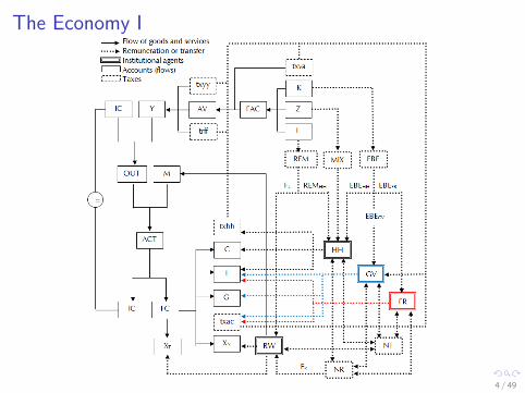
The Economy I

4 / 49

SAM

Bal.

B

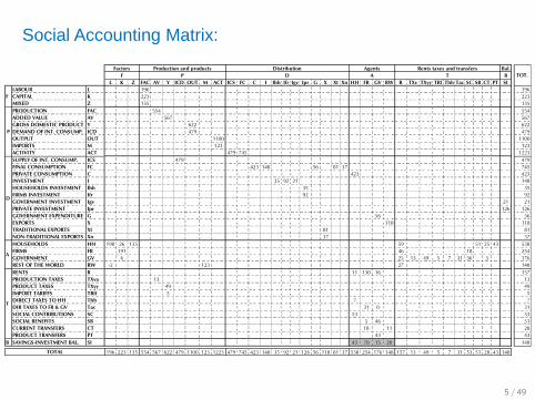
L K Z FAC AV Y ICD OUT M ACT ICS FC C I Ihh Ifr Igv Ipr G X Xt Xn HH FR GV RW R TXv TXyy TRf Thh Tac SC SB CT PT SI

LABOUR L 196 196

CAPITAL K 223 223

MIXED Z 135 135

PRODUCTION FAC 554 554

ADDED VALUE AV 567 567

GROSS DOMESTIC PRODUCT Y 622 622

DEMAND OF INT. CONSUMP. ICD 479 479

OUTPUT OUT 1100 1100

IMPORTS M 123 123

ACTIVITY ACT 479 745 1223

SUPPLY OF INT. CONSUMP. ICS 479 479

FINAL CONSUMPTION FC 423 148 56 81 37 745

PRIVATE CONSUMPTION C 423 423

INVESTMENT I 35 92 21 148

HOUSEHOLDS INVESTMENT Ihh 35 35

FIRMS INVESTMENT Ifr 92 92

GOVERNMENT INVESTMENT Igv 21 21

PRIVATE INVESTMENT Ipr 126 126

GOVERNMENT EXPENDITURE G 56 56

EXPORTS X 118 118

TRADITIONAL EXPORTS Xt 81 81

NON-TRADITIONAL EXPORTS Xn 37 37

HOUSEHOLDS HH 198 26 135 59 51 25 43 538

FIRMS FR 191 46 18 254

GOVERNMENT GV 6 25 13 49 5 7 31 36 3 176

REST OF THE WORLD RW -2 123 27 148

RENTS R 11 130 16 157

PRODUCTION TAXES TXva 13 13

PRODUCT TAXES TXyy 49 49

IMPORT TARIFFS TRff 5 5

DIRECT TAXES TO HH Thh 7 7

DIR TAXES TO FR & GV Tac 31 0 31

SOCIAL CONTRIBUTIONS SC 53 53

SOCIAL BENEFITS SB 5 46 51

CURRENT TRANSFERS CT 18 11 28

PRODUCT TRANSFERS PT 43 43

B SAVINGS-INVESTMENT BAL. SI 43 70 15 20 148

196 223 135 554 567 622 479 1100 123 1223 479 745 423 148 35 92 21 126 56 118 81 37 538 254 176 148 157 13 49 5 7 31 53 51 28 43 148

Agents

TOT.A T

Rents taxes and transfers

TOTAL

Production and products

F P D

P

D

A

T

DistributionFactors

F

Social Accounting Matrix:

5 / 49

The Model: Supply Side

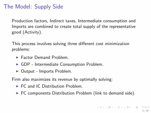
Production factors, Indirect taxes, Intermediate consumption andImports are combined to create total supply of the representativegood (Activity).

This process involves solving three different cost minimizationproblems:

I Factor Demand Problem.

I GDP - Intermediate Consumption Problem.

I Output - Imports Problem.

Firm also maximizes its revenue by optimally solving:

I FC and IC Distribution Problem.

I FC components Distribution Problem (link to demand side).

6 / 49

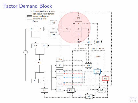
Factor Demand Block

7 / 49

The Model: Factor Demand Problem I

I Three factors combined + Production Taxes = Value Added.

I Firms solve the Factors Demand Problem (minimizesexpenditure subject to production):

min{L,K ,Z}

pLL + pKK + pZZ ,

s.t.

FAC = θF

(πLL

σF −1

σF + πKKσF −1

σF + πZZσF −1

σF

) σFσF −1

I Elasticity of substitution among factors satisfies σF > 0.

8 / 49

The Model: Factor Demand Problem II

From the FOCs we derive the optimal demand of factors:

L =

(θFπL

pF

pL

)σF FAC

θF, K =

(θFπK

pF

pK

)σF FAC

θF,

Z =

(θFπZ

pF

pZ

)σF FAC

θF,

where the aggregated price of factors pF is expressed as

pF =1

θF

(πσF

L p1−σFL + πσF

K p1−σFK + πσF

Z p1−σFZ

) 11−σF

9 / 49

The Model: Indirect taxes and GDP

I Added value, AV , is completed once indirect production taxesare acknowledged (nominal terms):

pAVAV = pFFAC + TXva ,

where tax revenue in production (TXva) is given by

TXva = txvapFFAC .

I GDP (Y ) supply is obtained by adding up AV, indirect (net)taxes over products (TXyy ) and import tariffs (TRff ):

pY Y = pAVAV + TXyy + TRff ,

where indirect product taxes and tariffs are given by

TXyy = txyypAVAV , and TRff = trff pMM

10 / 49

Domestic Supply Block

11 / 49

The Model: Domestic Output Problem I

I GDP and IC combined yield total domestic supply of therepresentative good.

I The firm solves for optimal combination of Y and IC in thedomestic output’s second-level cost minimization problem:

min{Y ,IC}

pY Y + pIC ICD

s.t.

OUT = θO

(πY Y

σO−1

σO + πICD ICDσO−1

σO

) σOσO−1

I Again, elasticity of substitution between Y and IC satisfyσO > 0, however, these goods are more complementary thansubstitutes (0 < σO < 1).

12 / 49

The Model: Domestic Output Problem II

I From FOCs, optimal GDP and Intermediate Consumptiondemands are

Y =

(θOπY

pO

pY

)σo OUT

θO, and ICD =

(θOπICD

pO

pIC

)σO OUT

θO,

where the aggregated price of domestic output pO is

pO =1

θO

(πσO

Y p1−σOY + πσO

ICDp1−σOIC

) 11−σO

I With Y’s Demand and Supply equations, one can solve for theprice of GDP, pY :

pY =

[pAVAV + TXyy + TRff

(θOπY pO)σO OUTθO

] 11−σO

13 / 49

Total Supply Block

14 / 49

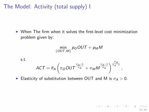
The Model: Activity (total supply) I

I When The firm when it solves the first-level cost minimizationproblem given by:

min{OUT ,M}

pOOUT + pMM

s.t.

ACT = θA

(πOOUT

σA−1

σA + πMMσA−1

σA

) σAσA−1

,

I Elasticity of substitution between OUT and M is σA > 0.

15 / 49

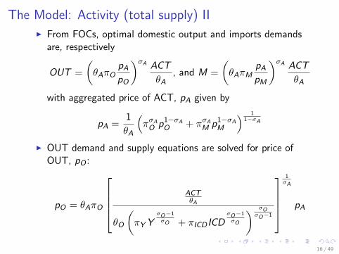
The Model: Activity (total supply) II

I From FOCs, optimal domestic output and imports demandsare, respectively

OUT =

(θAπO

pA

pO

)σA ACT

θA, and M =

(θAπM

pA

pM

)σA ACT

θA

with aggregated price of ACT, pA given by

pA =1

θA

(πσA

O p1−σAO + πσA

M p1−σAM

) 11−σA

I OUT demand and supply equations are solved for price ofOUT, pO :

pO = θAπO

ACTθA

θO

(πY Y

σO−1

σO + πICD ICDσO−1

σO

) σOσO−1

1σA

pA

16 / 49

The Model: Activity (total supply) III

Additional considerations on ACT formation:

I The clearing market condition assures that

pAACT = pOOUT + pMM.

I RW provides all demand for imports inelastically at theinternational price p∗M , and therefore

pM = ep∗M

where e is the nominal exchange rate.

17 / 49

Supply Distribution Block

18 / 49

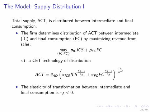
The Model: Supply Distribution I

Total supply, ACT, is distributed between intermediate and finalconsumption.

I The firm determines distribution of ACT between intermediate(IC) and final consumption (FC) by maximizing revenue fromsales:

max{IC ,FC}

pIC ICS + pFCFC

s.t. a CET technology of distribution

ACT = θAD

(πICS ICS

τA−1

τA + πFCFCτA−1

τA

) τAτA−1

I The elasticity of transformation between intermediate andfinal consumption is τA < 0.

19 / 49

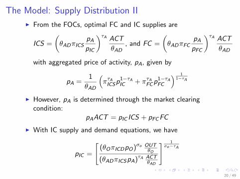
The Model: Supply Distribution II

I From the FOCs, optimal FC and IC supplies are

ICS =

(θADπICS

pA

pIC

)τA ACT

θAD, and FC =

(θADπFC

pA

pFC

)τA ACT

θAD

with aggregated price of activity, pA, given by

pA =1

θAD

(πτA

ICSp1−τAIC + πτA

FCp1−τAFC

) 11−τA

I However, pA is determined through the market clearingcondition:

pAACT = pIC ICS + pFCFC

I With IC supply and demand equations, we have

pIC =

[(θOπICDpO)σo OUT

θO

(θADπICSpA)τA ACTθAD

] 1σo−τA

20 / 49

FC Distribution Block

21 / 49

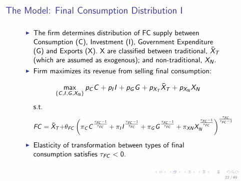
The Model: Final Consumption Distribution I

I The firm determines distribution of FC supply betweenConsumption (C), Investment (I), Government Expenditure(G) and Exports (X). X are classified between traditional, XT

(which are assumed as exogenous); and non-traditional, XN .

I Firm maximizes its revenue from selling final consumption:

max{C ,I ,G ,XN}

pCC + pI I + pGG + pXTXT + pXN

XN

s.t.

FC = XT +θFC

(πCC

τFC −1

τFC + πI IτFC −1

τFC + πGGτFC −1

τFC + πXNXτFC −1

τFC

N

) τFCτFC −1

I Elasticity of transformation between types of finalconsumption satisfies τFC < 0.

22 / 49

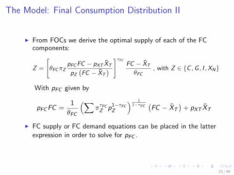
The Model: Final Consumption Distribution II

I From FOCs we derive the optimal supply of each of the FCcomponents:

Z =

[θFCπZ

pFCFC − pXT XT

pZ

(FC − XT

) ]τFC

FC − XT

θFC, with Z ∈ {C ,G , I ,XN}

With pFC given by

pFCFC =1

θFC

(∑πτFC

Z p1−τFCZ

) 11−τFC

(FC − XT

)+ pXT XT

I FC supply or FC demand equations can be placed in the latterexpression in order to solve for pFC .

23 / 49

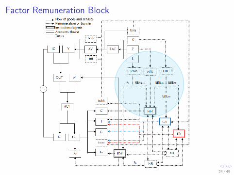
Factor Remuneration Block

24 / 49

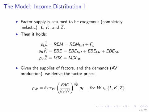
The Model: Income Distribution I

I Factor supply is assumed to be exogenous (completelyinelastic): L, K , and Z .

I Then it holds:

pLL = REM = REMHH + FL

pK K = EBE = EBEHH + EBEFR + EBEGV

pZ Z = MIX = MIXHH

I Given the supplies of factors, and the demands (AVproduction), we derive the factor prices:

pW = θFπW

(FAC

θF W

) 1σF

pF , for W ∈ {L,K ,Z}.

25 / 49

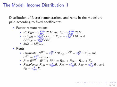
The Model: Income Distribution II

Distribution of factor remunerations and rents in the model arepaid according to fixed coefficients:

I Factor remunerations:I REMHH = πREM

HH REM and FL = πREMRW REM.

I EBEHH = πEBEHH EBE , EBEFR = πEBE

FR EBE andEBEGV = πEBE

GV EBE .I MIX = MIXHH .

I Rents:I Payments: RHH = πHH

R EBEHH , RFR = πFRR EBEFR and

RGV = πGVR EBEGV .

I R = RHH + RFR + RGV = RHH + RFR + RGV + FK .I Recipients: RHH = πR

HHR, RFR = πRFRR, RGV = πR

GVR , andFK = πR

RWR.

26 / 49

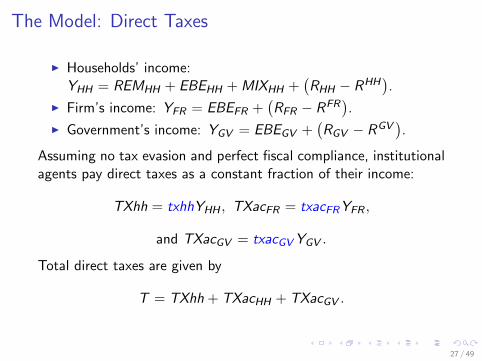
The Model: Direct Taxes

I Households’ income:YHH = REMHH + EBEHH + MIXHH +

(RHH − RHH

).

I Firm’s income: YFR = EBEFR +(RFR − RFR

).

I Government’s income: YGV = EBEGV +(RGV − RGV

).

Assuming no tax evasion and perfect fiscal compliance, institutionalagents pay direct taxes as a constant fraction of their income:

TXhh = txhhYHH , TXacFR = txacFRYFR ,

and TXacGV = txacGVYGV .

Total direct taxes are given by

T = TXhh + TXacHH + TXacGV .

27 / 49

The Model: Transfers I

There are four types of transfers: social contributions (SC), socialbenefits (SB), current transfers (CT), and product transfers (PT).

I We assume exogenous payments of social contributions SCHH

by HH, which is distributed FR and GV:

SCHHFR = πSC

FRSCHH

, and SCHHGV = πSC

GVSCHH.

I HH receive exogenously assumed social benefits, SB = SBHH ,from FR and GV:

SBFRHH = πSB

FRSBHH , and SBGVHH = πSB

GVSBHH .

I FR and RW pay CT exogenously, CTRW

+ CTFR

= CT ,which is distributed to HH and GV as:

CTHH = πCTHHCT , and CTGV = πCT

GVCT .

28 / 49

The Model: Transfers II

I We also assume exogenous product transfers from theGovernment to households, PTHH .

I Net transfers are then represented by the following equations:

NTHH = −SCHH+ SBHH + CTHH + PT

GVHH

NTFR = SCHHFR − SBFR

HH − CTFR

NTGV = SCHHGV − SBGV

HH + CTGV − PTGVHH

NTRW = −CTRW

29 / 49

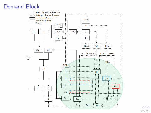
Demand Block

30 / 49

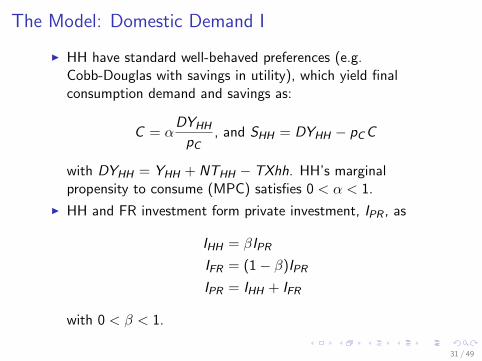
The Model: Domestic Demand I

I HH have standard well-behaved preferences (e.g.Cobb-Douglas with savings in utility), which yield finalconsumption demand and savings as:

C = αDYHH

pC, and SHH = DYHH − pCC

with DYHH = YHH + NTHH − TXhh. HH’s marginalpropensity to consume (MPC) satisfies 0 < α < 1.

I HH and FR investment form private investment, IPR , as

IHH = βIPR

IFR = (1− β)IPR

IPR = IHH + IFR

with 0 < β < 1.

31 / 49

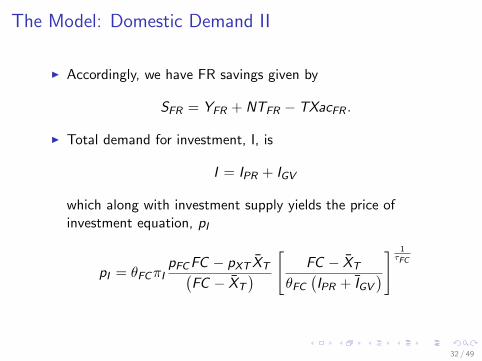
The Model: Domestic Demand II

I Accordingly, we have FR savings given by

SFR = YFR + NTFR − TXacFR .

I Total demand for investment, I, is

I = IPR + IGV

which along with investment supply yields the price ofinvestment equation, pI

pI = θFCπIpFCFC − pXT XT(

FC − XT

) [FC − XT

θFC

(IPR + IGV

)] 1τFC

32 / 49

The Model: Domestic Demand III

I We assume GV’s expenditure, G, and investment, IGV , to beexogenous:

G = G , and IGV = IGV

I GV expenditure price is jointly determined by its supply anddemand functions

pG = θFCπGpFCFC − pXT XT(

FC − XT

) (FC − XT

θFC G

) 1τFC

I Accordingly, GV savings are given by

SGV = YGV + NTGV + Tx + T − TXacGV − pG G

with indirect taxes Tx = TXva + TXyy + TRff .

33 / 49

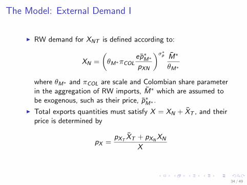
The Model: External Demand I

I RW demand for XNT is defined according to:

XN =

(θM∗πCOL

ep∗M∗

pXN

)σ∗p M∗

θM∗

where θM∗ and πCOL are scale and Colombian share parameterin the aggregation of RW imports, M∗ which are assumed tobe exogenous, such as their price, p∗M∗ .

I Total exports quantities must satisfy X = XN + XT , and theirprice is determined by

pX =pXT

XT + pXNXN

X

34 / 49

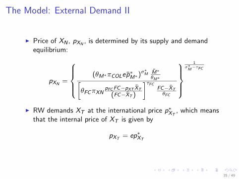
The Model: External Demand II

I Price of XN , pXN, is determined by its supply and demand

equilibrium:

pXN=

(θM∗πCOLep

∗M∗)σ

∗M M∗

θM∗[θFCπXN

pFC FC−pXT XT

(FC−XT )

]τFCFC−XTθFC

1

σ∗M

−τFC

I RW demands XT at the international price p∗XT, which means

that the internal price of XT is given by

pXT= ep∗XT

35 / 49

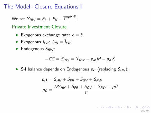
The Model: Closure Equations I

We set YRW = FL + FK − CTRW

.

Private Investment Closure

I Exogenous exchange rate: e = e.

I Exogenous IPR : IPR = IPR .

I Endogenous SRW :

−CC = SRW = YRW + pMM − pXX

I S-I balance depends on Endogenous pC (replacing SHH):

pI I = SHH + SFR + SGV + SRW

pC =DYHH + SFR + SGV + SRW − pI I

C

36 / 49

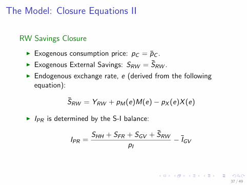
The Model: Closure Equations II

RW Savings Closure

I Exogenous consumption price: pC = pC .

I Exogenous External Savings: SRW = SRW .

I Endogenous exchange rate, e (derived from the followingequation):

SRW = YRW + pM(e)M(e)− pX (e)X (e)

I IPR is determined by the S-I balance:

IPR =SHH + SFR + SGV + SRW

pI− IGV

37 / 49

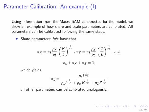
Parameter Calibration: An example (I)

Using information from the Macro-SAM constructed for the model, weshow an example of how share and scale parameters are calibrated. Allparameters can be calibrated following the same steps.

I Share parameters: We have that

πK = πLpK

pL

(K

L

) 1σF

, πZ = πLpZ

pL

(Z

L

) 1σF

and

πL + πK + πZ = 1,

which yields

πL =pLL

1σF

pLL1

σF + pKK1

σF + pZZ1

σF

all other parameters can be calibrated analogously.

38 / 49

Parameter Calibration: An example (II)

I Scale parameters: Using the share parameters and FAC, wehave

θF = FAC

pLL1

σF + pKK1

σF + pZZ1

σF

pLL + pKK + pZZ

σF

σF −1

39 / 49

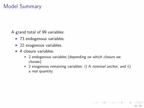
Model Summary

A grand total of 99 variables:

I 73 endogenous variables.

I 22 exogenous variables.I 4 closure variables:

I 2 endogenous variables (depending on which closure wechoose).

I 2 exogenous remaining variables: i) A nominal anchor, and ii)a real quantity.

40 / 49

Endogenous Variables

Endogenous Variables List (73)

FAC pF AV TXva pAV TXyy TRff YICD pY OUT M pO ACT pM ICS

FC pA pIC I XN pFC REM EBEMIX pL pK pZ REMHH FL EBEHH EBEFR

EBEGV RHH RFR RGV RHH RFR RGV FK

R YHH YFR YGV TXhh TXacFR TXacGV TSCHH

FR SCHHGV SBFR

HH SBGVHH CT CTHH CTGV NTHH

NTFR NTGV C SHH DYHH IHH IFR SFR

pI SGV Tx pG X pX pXNpXT

YRW .

41 / 49

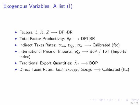
Exogenous Variables: A list (I)

I Factors: L, K , Z −→ DPI-BR

I Total Factor Productivity: θF −→ DPI-BR

I Indirect Taxes Rates: txva, txyy , trff −→ Calibrated (ftc)

I International Price of Imports: p∗M −→ BoP / ToT (ImportsIndex)

I Traditional Export Quantities: XT −→ BOP

I Direct Taxes Rates: txhh, txacFR , txacGV −→ Calibrated (ftc)

42 / 49

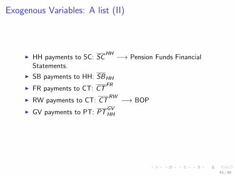
Exogenous Variables: A list (II)

I HH payments to SC: SCHH −→ Pension Funds Financial

Statements.

I SB payments to HH: SBHH

I FR payments to CT: CTFR

I RW payments to CT: CTRW −→ BOP

I GV payments to PT: PTGVHH

43 / 49

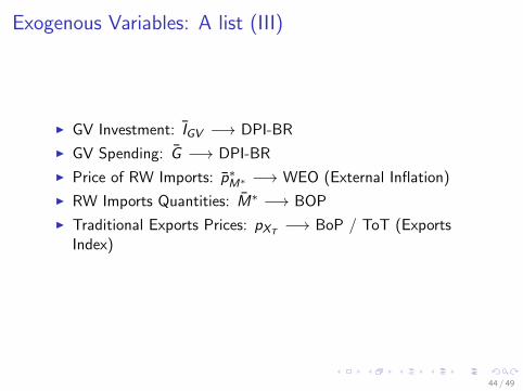
Exogenous Variables: A list (III)

I GV Investment: IGV −→ DPI-BR

I GV Spending: G −→ DPI-BR

I Price of RW Imports: p∗M∗ −→ WEO (External Inflation)

I RW Imports Quantities: M∗ −→ BOP

I Traditional Exports Prices: pXT−→ BoP / ToT (Exports

Index)

44 / 49

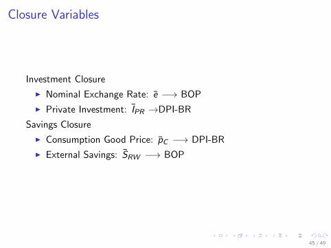
Closure Variables

Investment Closure

I Nominal Exchange Rate: e −→ BOP

I Private Investment: IPR →DPI-BR

Savings Closure

I Consumption Good Price: pC −→ DPI-BR

I External Savings: SRW −→ BOP

45 / 49

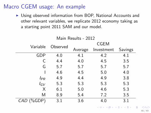
Macro CGEM usage: An example

I Using observed information from BOP, National Accounts andother relevant variables, we replicate 2012 economy taking asa starting point 2011 SAM and our model.

Main Results - 2012

Variable ObservedCGEM

Average Investment Savings

GDP 4.0 4.1 4.2 4.1C 4.4 4.0 4.5 3.5G 5.7 5.7 5.7 5.7I 4.6 4.5 5.0 4.0

IPR 4.9 4.4 4.9 3.8IGV 5.3 5.3 5.3 5.3

X 6.1 5.0 4.6 5.3M 8.9 5.4 7.2 3.5

CAD (%GDP) 3.1 3.6 4.0 3.1

46 / 49

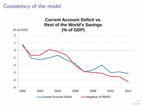
Consistency of the model

-5

-4

-3

-2

-1

0

1

2

2000 2002 2004 2006 2008 2010 2012

(% of GDP)

Current Account Deficit vs.Rest of the World's Savings

(% of GDP)

Current Account Deficit Negative of RWSV

47 / 49

What’s Next?

This model can be further extended along the following lines:

I Demand driven economy.

I Assuring BoP matching with the model.

I Multi-sector CGE model.

I Extension of Fiscal Block.

I Money in CGEM (anchor to Monetary accounts).

48 / 49

THE END

Thank You.

49 / 49