a low-complexity architecture and framework for enabling
TRANSCRIPT

A LOW-COMPLEXITY ARCHITECTURE AND FRAMEWORK
FOR ENABLING COGNITION IN HETEROGENEOUS WIRELESS
SENSOR NETWORKS
by
Parisa Abedi Khoozani
A thesis submitted to the Department of Electrical and Computer Engineering
In conformity with the requirements for
the degree of Master of Applied Science
Queen’s University
Kingston, Ontario, Canada
(February, 2013)
Copyright ©Parisa Abedi Khoozani, 2013

ii
Abstract
Rapid advances in hardware technology are making it possible to manufacture different types of
Sensor Nodes (SN) that results in fast growing heterogeneous Wireless Sensor Networks
(WSNs). These WSN’s are applicable for a wide range of applications relevant for military,
industry and domestic use. However, WSNs have particular features such as scarce resources
which can affect their performance. In addition, WSNs are subject to experience changes that can
occur both within the condition of the network, due to factors such as node mobility or node
failure (prevalent in harsh environments), and with regards to user requirements. Consequently, it
is vital for WSNs to sense the current network conditions and user requirements to be able to
perform efficiently. Cognition is necessarily introduced in WSNs as a response to this need.
Cognition in the context of WSNs deals with the ability to be aware of the environment and user
requirements and to proactively adapt to changes.
This thesis proposes a hierarchical architecture along with a cognitive network management
protocol capable of enabling cognition in WSNs. Specifically; this research introduces Cognitive
Nodes (CN) into WSNs so that they can manage the cognitive network. The cognitive network
management process is composed of three sub-processes: 1) scanning the network, 2) decision-
making, and 3) updating the nodes from taken decisions.Scanning the network process aims to
provide an awareness of current network conditions. Therefore, at the first execution, each CN
creates a profile table for each node in its purview and updates the tables periodically during the
network operation. In decision making process, CNs make necessary decisions in terms of the
working state of SNs (active/sleep), the duration of this state, and the Frequency of Sensing
(FoS). Decision making process uses an optimization scheme to find the optimal number of active
SNs in order to prolong the lifetime of the network. Finally, the nodes will be informed of the
taken decisions. Based on the simulation and implementation results, the proposed cognitive
WSN shows a significant enhancement in terms of the network’s longevity, its ability to negotiate
competing objectives, and its ability to serve users more efficiently.

iii
زم،یعز مادر و پدر به میتقد
زمیعز خواهر و

iv
Acknowledgements
First of all, I thank ALLAH (GOD) for his countless blessings without which this thesis would
not have been made possible.
I would like to thank Professor Mohamed Ibnkahla for his guidance and support and for letting
me work in his lab for the past two years. I have benefitted greatly as a student from working with
him.
I would like to thank Fadi M. Al-Turjman for his useful comments and Amr El Mougy for his
mentorship and constant insight throughout my time at Queen’s.
I am grateful to my dearest friends, Fereshteh Aalamifar and Saeed Akhavan Astaneh, for their
reviews, helpful comments, and supports throughout the writing of my thesis.
I want to thank all the members of WISIP lab and the ECE department for their help and feedback
throughout my studies.
I would like to thank Victoria Niva Millious for all her help and editing of this thesis.
Finally, I would like to thank and dedicate my work to my parents and to my dearest sister for
their love and support.

v
Table of Contents
Abstract ............................................................................................................................................ ii
Acknowledgements ......................................................................................................................... iv
Chapter 1 Introduction ..................................................................................................................... 1
1.1 Wireless Sensor Networks: Features, Challenges, and Applications ..................................... 1
1.2 Cognitive WSNs: Motivation and Scope ............................................................................... 4
1.3 Thesis Contribution ................................................................................................................ 5
1.4 Thesis Outline ........................................................................................................................ 7
Chapter 2 Background and Literature Review ................................................................................. 8
2.1 Design Factors in WSNs ........................................................................................................ 8
2.1.1 Coverage ......................................................................................................................... 9
2.1.2 Connectivity .................................................................................................................. 10
2.1.3 Lifetime ......................................................................................................................... 10
2.1.4 QoS Support in WSN .................................................................................................... 11
2.2 Different Approaches in Improving WSNs Performance .................................................... 12
2.2.1 Energy-aware Protocols ................................................................................................ 12
2.2.2 Cross-Layer Design ...................................................................................................... 15
2.2.3 Cognitive-Based Approaches ........................................................................................ 17
2.2.3.1 Implementing Cognition Partially .......................................................................... 18
2.2.3.2 Implementing Cognition Globally ......................................................................... 20
2.3 Summary- a Comparison ..................................................................................................... 22
Chapter 3 System Architecture and Models .................................................................................. 24
3.1 System Architecture ............................................................................................................. 24
3.1.1 Standards ....................................................................................................................... 24
3.1.1.1 IEEE 802.15.4 Summary ....................................................................................... 24
3.1.1.2 ZigBee Summary ................................................................................................... 27
3.1.2 System Components ...................................................................................................... 27
3.1.3 Node Deployment ......................................................................................................... 29
3.1.4 The Proposed Architecture............................................................................................ 30
3.2 System Models ..................................................................................................................... 33
3.2.1 Coverage Model ............................................................................................................ 33
3.2.2 Lifetime Model ............................................................................................................. 34
3.2.2.1 Power Consumption Model ................................................................................... 34
3.2.3 Communication Model ................................................................................................. 35

vi
3.2.3.1 Propagation Model ................................................................................................. 35
3.2.4 Network Model ............................................................................................................. 36
Chapter 4 Cognitive Network Framework ..................................................................................... 37
4.1 System Overview ................................................................................................................. 37
4.2 Cognitive Network Management Process ............................................................................ 39
4.2.1 Scanning the Network ................................................................................................... 40
4.2.1.1 SNs’ Profile Table .................................................................................................. 41
4.2.1.2 R/CHs’ Profile Table ............................................................................................. 42
4.2.1.3 Targets’ Profile Table ............................................................................................ 43
4.2.1.4 CNs’ Profile Table ................................................................................................. 43
4.2.2 Decision-making Process .............................................................................................. 44
4.2.2.1 Problem Statement and Contribution ..................................................................... 45
4.2.2.2 Determining Frequency of Sensing (FoS) ............................................................. 46
4.2.2.3 Maximum Set Cover (MSC) Problem Definition and Formulization .................... 50
4.2.2.4 Linear Programming Solution ................................................................................ 56
4.2.2.5 Greedy Solution ..................................................................................................... 58
4.2.3 Updating the Nodes from Taken Decisions .................................................................. 60
4.3 Graphical User Interface for WSN....................................................................................... 60
Chapter 5 Performance Evaluation ................................................................................................ 64
5.1 Simulation Setup .................................................................................................................. 64
5.2 Evaluation Metrics ............................................................................................................... 67
5.2.1 Network’s Lifetime ....................................................................................................... 67
5.2.2 Runtime Complexity of Algorithms ............................................................................. 67
5.2.3 Throughput and Packet Loss Ratio ............................................................................... 68
5.2.4 Battery Distribution ...................................................................................................... 68
5.2.5 Different Simulation Scenarios and Results ................................................................. 68
5.3 Experimental Setup and Results .......................................................................................... 86
Chapter 6 Conclusions and Future Works ..................................................................................... 90
6.1 Conclusions .......................................................................................................................... 90
6.2 Future Works ....................................................................................................................... 91
References ...................................................................................................................................... 93
Appendix A Pseudo Code and Flowchart of LP solution .............................................................. 97
Appendix B Pseudo-code and flow chart of Greedy Solution ....................................................... 99

vii
List of Figures
Figure 1.1. Different sensors necessary in a WSN used for highway safety ................................... 3
Figure 1.2. Different possible customers of a WSN used for highway safety ................................. 3
Figure 2.1. Cognitive Network Framework ................................................................................... 18
Figure 3.1. Different topologies in IEEE 802.15.4 ........................................................................ 26
Figure 3.2. A square area with four CNs ....................................................................................... 30
Figure 3.3. The Multitier network .................................................................................................. 32
Figure 3.4. The complete architecture of the system ..................................................................... 33
Figure 4.1. System transition diagram ........................................................................................... 38
Figure 4.2. Network states ............................................................................................................. 39
Figure 4.3. Discharge characteristics of the used battery .............................................................. 47
Figure 4.4. Mapping the FoS range to the discharge characteristic diagram ................................. 47
Figure 4.5. Critical points .............................................................................................................. 48
Figure 4.6. Relationship between FoS and BL .............................................................................. 48
Figure 4.7. A sample of the network with 5 SNs and 3 target points ............................................ 50
Figure 4.8. Two possible cover sets ............................................................................................... 51
Figure 4.9. A snapshot of the GUI program .................................................................................. 61
Figure 5.1. Nodes’ arrangement in the simulator ........................................................................... 66
Figure 5.2. Network’s lifetime ....................................................................................................... 70
Figure 5.3. Mean of the distribution of remaining battery of SNs ................................................. 71
Figure 5.4. Standard deviation of the distribution of remaining battery of SNs ............................ 72
Figure 5.5. Distribution of remaining battery ................................................................................ 73
Figure 5.6. Network management runtime .................................................................................... 73
Figure 5.7. Runtime for Cgreedy-MSC and greedy-MSC ............................................................. 74
Figure 5.8. Network Lifetime ........................................................................................................ 76
Figure 5.9. Average percentage of coverage .................................................................................. 77
Figure 5.10. Network lifetime ........................................................................................................ 79
Figure 5.11. Average of throughput in different links ................................................................... 80
Figure 5.12. Average of PLR in different links ............................................................................. 80
Figure 5.13. Network management runtime for all four algorithms .............................................. 81
Figure 5.14. Runtime of network management for the two greedy algorithms ............................. 82
Figure 5.15. Average of the distribution of remaining battery for all four algorithms .................. 83
Figure 5.16. Average of the distribution of remaining battery for weighted algorithms ............... 83
Figure 5.17. Average of the distribution of remaining battery for non-weighted algorithms ........ 84

viii
Figure 5.18. Standard deviation of the distribution of remained battery for all four algorithms ... 84
Figure 5.19. Standard deviation of the distribution of remaining battery for weighted algorithms
....................................................................................................................................................... 85
Figure 5.20. Standard deviation of the distribution of remaining battery for non-weighted
algorithms ...................................................................................................................................... 85
Figure 5.21. Implementation setup ................................................................................................ 87
Figure 5.22. Lifetime of Cognitive WSN vs. Non-Cognitive WSN .............................................. 88
Figure 5.23. Designed GUI with current information of a sample Network ................................. 89
Figure 7.1. Flowchart of implemented LP algorithm ..................................................................... 98
Figure 7.2. Flowchart of implemented greedy algorithm ............................................................ 100

ix
List of Tables
Table 2.1. Comparison of approaches ............................................................................................ 23
Table 4.1. SNs’ profile table .......................................................................................................... 42
Table 4.2. R/CHs’ Profile Table .................................................................................................... 43
Table 4.3. Targets’ profile table ..................................................................................................... 43
Table 4.4. CNs’ profile table .......................................................................................................... 44
Table 4.5. FoS table used in the experiment .................................................................................. 49
Table 5.1. Simulation parameters – area and number of nodes ..................................................... 66
Table 5.2. Simulation parameters – communication and sensing ranges ...................................... 66
Table 5.3. Simulation parameters – physical parameters ............................................................... 67

x
List of Acronyms WSN Wireless Sensor Network
SN Sensor Node
CWSN Cognitive Wireless Sensor Network
MAC Medium Access Control
CN Cognitive Node
MINA Multi-hop Infrastructure Network Architecture
QoS Quality of Service
GAF Geographical Adaptive Fidelity
TRAMA Traffic-Adaptive Medium Access
TDMA Time Division Multiple Access
KP Knowledge Plane
KB Knowledge Base
SDT Sensory Data Transmission
PHY Physical Layer
FFD Full Function Device
RFD Reduced Function Device
PAN Personal Area Network
CH Cluster Head
CID Cluster Identification
CSMA/CA Career Sense Multiple Access/ Collision Avoidance
ACK Acknowledgement Packet
PER Packet Error Rate
R/CH Router/Cluster Head
BL Battery Level
UF Utility Factor
SID Sensor Identification
FoS Frequency of Sensing
PLR Packet Loss Ratio
MSC Maximum Set Cover
FL Flow Rate
LP
NFP
GUI
Linear Programming
Node Failure Probability
Graphical User Interface

1
Chapter 1
Introduction
Wireless Sensor Networks (WSNs) are growing rapidly and emerging as a promising solution for
a wide range of applications pertaining to military, home, environmental, health, industrial
automation, and highway safety. A WSN consists of a group of small nodes equipped with short-
range communication capabilities, which are densely distributed in a particular area to measure
certain phenomena such as humidity, air pressure, and temperature. Each node is composed of
four parts: a sensing unit, a processing unit, a power unit, and a transceiver. The nodes are small
in size, therefore they are resource-limited, i.e. power, memory, and processing capability are
scarce. As a result, it is necessary to design WSNs carefully to meet their unique expected
objectives, such as throughput, lifetime, connectivity, and coverage [1]-[2].
1.1 Wireless Sensor Networks: Features, Challenges, and Applications
A WSN is characterized by the following features [1]-[2]:
1. Low capacity (in terms of memory, CPU, and battery): as the nodes are small in size and
must be cost effective.
2. Low data rate: the available bandwidth is limited.
3. Scalable: a huge number of nodes are distributed in the interested area.
4. Fault tolerant: since such networks can be deployed in harsh environments, the
probabilities of node failure and link failure are high. Thus, the network must be able to
continue working if a node or a link fails. In the case of node failure, others nodes
(backup nodes or other active nodes) can carry out the duties of the failed node(s). In the

2
case of link failure, nodes must be able to establish and maintain communications
between each other.
There are certain issues that must be addressed when designing a WSN:
1. Network longevity: As mentioned before, WSN batteries are limited and it is important to
design energy efficient protocols for such networks.
2. Coverage: As the sensing range of each sensor is limited, it is necessary to distribute
enough Sensor Nodes (SNs) in order to ensure that each area in the region of interest is,
at minimum, within the sensing range of one SN.
3. Network connectivity: Connectivity means that the Sink Node is reachable for employed
nodes.
In addition to the above-mentioned issues, recent and rapid advances in hardware technology now
make it possible to manufacture different types of sensors. Thus, WSNs can possess multiple
sensors with distinct characteristics. This heterogeneous nature brings new challenges to the fore.
As each sensor has different characteristics, it is important to consider the variant features of each
sensor when designing protocols and architecture. Furthermore, the customers who use the data
provided by the WSNs may have unique requirements; these must be addressed. Figure 1.1 and
Figure 1.2 illustrate such examples of different sensors and different possible customers of a
WSN respectively.

3
Figure 1.1. Different sensors necessary in a WSN used for highway safety
Figure 1.2. Different possible customers of a WSN used for highway safety

4
1.2 Cognitive WSNs: Motivation and Scope
WSNs are subject to experience changes in both network conditions, due to factors such as
mobility and node failure (e.g. in harsh environments), and also user requirements (e.g. rate of
data transmission). Traditional architectures and protocols proposed for WSNs are not capable of
adapting themselves to such unstable network conditions. Furthermore, most of the protocols of
WSNs are either suited solely for homogenous networks or demand a problematically dense
complexity when the network is heterogeneous. Therefore, there is a need to develop new
architectures and protocols for WSNs. Cognitive WSNs (CWSNs) are introduced in response to
this need.
Based on the presented definition in [4]-[5], a cognitive network is a network with a cognitive
process that can perceive live network conditions, formulate an informed response, and react as
needed to secure the functionality and overall survival of the network. The network can, also,
learn from its previous decisions and apply these in future problem solving. Therefore, a CWSN
must be aware of the status of the nodes (asleep/active), the amount of generated sensory data, the
correct node and time to forward data. To do so, the available resources in each node, the network
status at MAC layer, and application requirements at application layer are gathered for use in the
decision making process. Consequently, by enabling cognition in WSNs, networks will be aware
of environmental changes, network status, and user requirements, and can adapt themselves to the
changes in order to satisfy user requirements. In this thesis, we propose a novel architecture and
cognitive network management algorithm for enabling cognition in WSNs with the goal to

5
improve the performance of WSNs. In the proposed CWSN, we shall consider full connectivity,
full coverage, lifetime, and user satisfaction.
1.3 Thesis Contribution
To clarify the contribution of this thesis, we first provide an example case where application of
CWSNs can be found: Highway safety. In this application, in order to collect enough information,
several types of sensors are deployed in the area of interest.
In highway safety applications, microwave radar, active/passive infrared, ultrasound, acoustic
array, magnetic Sensing, video/image processors, inductive loop detectors, fog sensors, humidity
and air pollution sensors, and temperature sensors can be used to produce intersectional control,
freeway incident detection, traffic congestion monitoring, ramp and freeway-to-freeway metering,
lateral control, traffic data collection, and weather and highway condition detection [29]. It is
common that in some parts of the road the probability of accidents is higher; reasonably, those
sections require additional monitoring and control. The algorithms should be able to amass and
hold the critical data and act quickly. For instance, if a speed detection sensor detects a vehicle
moving at a high speed, the camera should automatically turn-on to capture visuals of the vehicle.
Otherwise the camera can remain off, as it consumes a lot of energy and would otherwise require
additional bandwidth. However, in order to capture the critical data, the camera needs to be
activated fast enough.
Thus, the goal of the cognitive algorithm is to decide which sensor requires activation, when it
should be activated and for what duration of time it should work by considering the current
condition of the network, as well as the user requirements. In addition, the network should be

6
sufficiently malleable to allow users to adjust their requirements as needed. The contribution of
this thesis can be listed as following: We
1. Propose a new architecture for implementing cognition in WSN. It is important to
carefully design the network so that cognition is carefully merged within the network.
This is because cognition requires extra resources, such as energy and memory, which is
scarce in WSNs. Therefore, in this thesis we present a multi-tier network in which each
node has a specific responsibility. A new node, named Cognitive Node (CN), is added for
cognitive responsibilities.
2. Propose a low-complexity cognitive algorithm. In order to have a cognitive WSN, both
the architecture and the protocols should be designed carefully. As a result, we propose a
new cognitive algorithm which is able to adapt itself to the network situation and manage
and schedule different nodes based on their capabilities. We consider a heterogeneous
network that consists of several types of sensors with different characteristics and
customers with different requirements.
3. Experimentally implement the network with wireless nodes to evaluate its performance
by considering restrictions of real.
Thus, in summary, the aim of this thesis is to engineer a new architecture and protocol that
enables cognition for heterogeneous WSNs. As a result of such cognition, the network is aware of
its condition and of its user requirements and can adapt itself as needed.
7
1.4 Thesis Outline
In the following, an overview of the thesis will be presented. Chapter 2 provides a literature
review of similar and precedent work. The review explains different approaches in improving the
performance of WSNs as well as explaining the importance of the cognitive-based approaches.
An overview of a CWSN, Different system elements, node deployment method, and system
architecture as well as system models are provided in chapter 3. Chapter 4 explains the proposed
cognitive network management algorithm. In chapter 5, the details of the simulation setups are
described. The performance of the proposed system is evaluated by comparing the system with
the proposed algorithm in [24] – Multi-hop Infrastructure Network Architecture (MINA). To
evaluate the system fairly, we added our system scheduler algorithm to MINA and named it
improved-MINA. Finally, an overarching evaluation of the thesis work comprises the conclusion
in chapter 6, followed by an outline of potential future research.

8
Chapter 2
Background and Literature Review
A significant amount of research has been done on different aspects of WSNs including their
architecture, protocol designs, energy conservation, and deployment strategies. However, these
techniques (or, ‘overall, this body of research falls short methodologically by failing to
adequately address the following) suffer from two important shortcomings:
1) Inability to optimize multiple goals and balance among them
2) Inability to adapt to the network and changes in user-requirements
Cognition was introduced to WSNs to overcome the above-mentioned shortcomings. In [4]-[5],
Thomas et al introduced the idea of cognition in a general network. The authors defined a
cognitive network as a proactive network, which is aware of its network conditions and end-to-
end goals. Such a network can adapt itself to the current condition of the network in order to
satisfy the end-to-end goals. It, also, is able to learn from previous decisions and use them
towards future decisions.
To be able to understand the importance of Cognition in WSNs and challenges ahead, in this
chapter we review different attempts for improving the WSNs performance as well as cognitive-
based approaches, along with their advantages and disadvantages. To this end first design factors
in WSNs are explained.
2.1 Design Factors in WSNs
WSNs are constructed by a huge number of sensor nodes distributed in the area of interest. The
deployed nodes are limited in power, processing capacity, and storage. In addition, the
communication range and sensing range is limited. Consequently, in order to improve system

9
performance and network efficiency it is important to consider several factors for designing
WSNs.
The first issue in WSNs is node deployment which is the process of determining the numbers and
positions of the utilized nodes in the field of interest. In literature, node deployment can be
classified in two categories: deterministic and random. In random deployment, the node will be
distributed randomly in field of interest while in deterministic deployment each node has a
predefined position [38]-[39].
We classified design factors in two categories: primary and secondary. Primary factors are
lifetime, coverage, and connectivity, while secondary factors are scalability and fault tolerance.
All factors are briefly explained in chapter 1. In the following we provided more explanation for
primary factors. As the design factors can be used to evaluate the Quality of Service (QoS) in
WSN, the QoS in WSNs is provided in section 2.1.4.
2.1.1 Coverage
Coverage can be defined as “how well the field of interest is monitored by employed SNs”. In
other word, the goal is to monitor each location in field of interest within the sensing range of at
least one SN. The sensing range can be a uniform disk of radius rs or a probabilistic sensing
model. In the uniform disk model all the events at a distance equal or less than rs from SN will be
detected by the SN. While events occurring at distance rs+ ( 0 ) cannot be detected at all
[40]-[41]. In contrast, in the probabilistic model detection of an event is based on a probabilistic
function of the distance from SN [42].

10
K-coverage is introduced to increase the reliability of the sensed data. The goal is to monitor each
location of the area of interest by at least k SNs [43]. Another factor in measuring the coverage is
what you are attempting to cover: an entire area or a set of targets.
2.1.2 Connectivity
Connectivity in WSNs is defined as “the ability of reaching the Sink Node from each node in the
network”, therefore it is essential to ensure that there is at least a path to the Sink Node from each
node (network satisfies full connectivity) [44]. Connectivity can be presented as k-connectivity
which means there are at least k independent path between each deployed node and the Sink
Node [45].
It is beneficial to mention that some researchers used different meaning for k-connectivity: there
are at least k independent link between each node and Sink Node. However, the k-link
connectivity does not guarantee the full network connectivity [46]-[47].
2.1.3 Lifetime
Prolonging network lifetime is the most challenging problem in WSNs, as the available power is
limited in utilized nodes and nodes replacement or recharging is not feasible. Accordingly, it is
required to consider energy efficiency while designing any architecture or protocol for WSNs.
Network lifetime has several definitions in literature [48]-[49]. One of the most common
definitions is the time span from network deployment until the first node death occurs. However,
this definition may not be suitable for all applications. For example, in monitoring application
(such as monitoring the temperature of a highway) as long as we can receive information about
every targeted area, the network can be considered as operational even though some nodes are

11
dead. Similarly, using the definition in which last node death is considered as the time that the
network is not operational is not appropriate [50].
Another way is to define lifetime based on the percentage of nodes which are alive. However, if
specific objectives (e.g. k-connectivity) have been considered for application, this definition is
not suitable too. Therefore, it is necessary to have an appropriate definition based on the
objectives of the networks. For example, time span from network deployment until the network is
partitioned or there is at least one uncovered target point.
2.1.4 QoS Support in WSN
It is necessary to present the Quality of Service (QoS) in WSNs and to clarify the concept of QoS
as it pertains to this research as different intellectual communities may hold contrasting
interpretations about QoS. Simply put, we consider QoS as a means of measuring user
satisfaction.
From the perspective of network engineers, the goal is to provide QoS (satisfy users) while
maximizing resource utilization. However, in WSNs, unlike traditional networks, the goal is not
solely optimum bandwidth utilization but also energy awareness. Therefore, because of the
specific features of WSNs, such as limited resources (battery, memory, and processing
capabilities) and high probability of topology variation (due to factors such as node and link
failure and mobility), some new QoS parameters should be defined and added to the QoS
requirements of traditional networks. QoS in WSNs can be classified in two categories [6]:
Application-specific QoS: WSNs can be used in a variety of applications and each
application has its own requirements. Deployment strategies, coverage, optimum number

12
of active sensors, and user classification (e.g. the availability of services such as data rate
and delay to the users based on their priority level) are categorized in this class of QoS.
Network QoS: Parameters related to the quality of data delivery compose this category.
The parameters that are important for WSNs are delay, throughput, packet loss, and
bandwidth utilization.
In the following, we clarify whether or not an approach contains any QoS parameters and how the
QoS is addressed in that algorithm.
2.2 Different Approaches in Improving WSNs Performance
2.2.1 Energy-aware Protocols
In most of the applications, because of the harsh environment, nodes are not feasibly accessible
and, therefore, energy awareness is one of the most important issues. Energy efficiency has been
addressed through different techniques such as finding the optimum number of active SNs (or
scheduling SNs’ activities), energy efficient routing protocols (i.e. finding the most efficient path
for forwarding the data), and energy efficient MAC protocols (e.g. by avoiding collision).
1. Finding the optimum number of active SNs: As SNs are small in size and inexpensive,
several SNs may be distributed in the area of interest and there may be more than one SN
covering a specific target. The logic behind these algorithms is to remove redundant data
by provoking the redundant SNs covering the same target into sleep mode. To this end, a
variety of objectives should be weighed and considered, such as connectivity, coverage,
and prolonging the network’s lifetime.
Some algorithms considered the coverage issue. These algorithms must be able to
maintain coverage while scheduling the SNs. In [7], the authors proposed an algorithm

13
for creating set covers. A set cover contains several SNs such that full coverage of the
network is guaranteed; there is at least one SN to cover each target. The set covers will be
constructed before the network deployment and the calculated schedule will be uploaded
on SNs. The authors in [7] proposed two algorithms to maximize the lifetime of the
network while maintaining the coverage, given the limited available battery capacity: 1) a
linear programming algorithm and 2) a greedy algorithm.
If the SNs are intended to cooperate to forward data, the connectivity of the network has
to be addressed. In [8], both connectivity and coverage are considered in the scheduling
process. The proposed algorithm is able to guarantee a certain degree of coverage and full
connectivity. However, the drawback of the algorithm is that it does not consider network
lifetime as a constraint and therefore does not seek to minimize energy consumed.
In [9], a near-optimal plan for WSNs - one that guarantees energy efficiency, full
coverage, and full connectivity - is presented. The nodes in the network can work in
three states: active, sleep, and cluster head. The algorithm seeks to determine the node’s
state while maintaining the coverage and full connectivity. A tabu-based algorithm,
which tries to find the optimum solution by performing a local search among the potential
solutions, computes the configurations of the network. The proposed algorithm in [9] has
a low computation time which is appropriate for large-scale networks. However, the
algorithm is not adaptive to the network changes, such as changes in topology or user
requirements.
From the QoS perspective, the algorithms of this category are mostly concerned with
providing application-specific QoS, i.e. coverage and connectivity.

14
2. Energy efficient Routing protocols: The goal in Routing protocols in WSNs is to find
the most efficient path, with regards to energy and latency, to the Sink Nod. Routing
protocols can have effects on both application-specific QoS, such as connectivity and
coverage, and on network QoS, such as latency and packet loss ratio [10].
As an example: Geographic Adaptive Fidelity (GAF) is an energy aware location based
routing protocol which can be used for mobile ad-hoc networks as well as WSNs [11]. It
forms a virtual grid by dividing the network into equal square zones. Each node is
assigned to a zone in the grid based on its position. The GAF tries to minimize the
number of intermediate nodes in forwarding data to the destination and therefore
minimizing the energy consumed by forwarding the data. The drawback of this algorithm
is the possibility of having to choose a node for more than one path and consequently the
possibility of having bottleneck in the network.
3. Energy efficient MAC protocols: Since the transmission and reception are the most
energy consuming phenomena in nodes, it is important to avoid unnecessary
transmission/reception. Therefore, in order to have energy efficiency the number of
retransmission due to collisions (when two packets are simultaneously received),
overhearing (when a node receives a packet belongs to another node), and overemitting
(when a packet is sent without considering the destination is not ready for receiving the
packet) should be reduced. In addition, since the nodes waste a lot of energy in idle
mode while they wait for upcoming traffic, a good solution is to reduce the idle time in
nodes. [12]
From the QoS point of view, MAC protocols are more involved in supporting network
QoS (such as avoiding delays and improving bandwidth allocation, throughput, and

15
packet loss ratio) rather than application-specific QoS. However, decreasing the idle time
in nodes is one of the application-specific QoS that has been addressed in MAC
protocols.
Literature [13] presents a Traffic-Adaptive Medium Access protocol (TRAMA). The
protocol reduces energy consumption by preventing occurring collisions in unicast and
broadcast communications. In addition, it allows nodes with no upcoming traffic to
change their state to a low-power mode. TRAMA uses Time Division Multiple Access
(TDMA) and assigns a time slot to each node by using a distributed election scheme in
which the time slots are assigned to nodes based on their upcoming traffic information.
TRAMA has a better lifetime and less packet loss ratio in comparison to contention-
based and static scheduled-access protocols. However, it suffers from a higher delay in
comparison to the contention-based protocols.
2.2.2 Cross-Layer Design
Since improving the parameters of one layer in a protocol stack can have inverse effects on the
performance of other layers, the separate improvement of parameters of different layers within a
protocol stack is not an optimal approach. Therefore, Cross-layer designs aims to improve the
performance of the network by sharing the information among different, but not necessarily
adjacent, layers.
Both application-specific and network QoS can be considered in this approach. However, for the
application-specific QoS, the user classification is not addressed which means that the network is
unable to provide service for the users based on their priority level.

16
Hithesh el al [14] presented a new algorithm to optimally set source rates, network flows, and
radio resources at the transport, network, and radio resource layers, sequentially, for jointly
maximizing the utility and lifetime of the network. The authors sought to provide a trade-off
between network lifetime and the application performance. They considered an orthogonal link
transmission in the network. The cross-layer optimization problem for determining the source
rates, network flows, and radio resources is formulated and it is shown by using dual
decomposition techniques that the problem can be reformulated as three sub-problems: a joint
transport and routing problem, a radio resource allocation problem, and a prolonging network
lifetime problem. Therefore, users are able to specify a threshold for optimization objectives, e.g.
lifetime and throughput. The result is that the algorithm capably achieves the threshold for the
specified optimization objectives.
As efficient energy consumption is the primary goal in WSNs, the authors in [15] proposed a
joint routing, MAC, and link layer optimization algorithm for WSNs with energy constraints.
They considered two sources of energy consumption in a node: consumption related to
transmission of data, and to circuit processing. The proposed energy efficient joint routing,
scheduling, and link adaptation algorithm determines the optimal slot length of the variable
TDMA MAC. In the first set of experiments, the algorithm was run solely for joint routing and
MAC. It was observed that the multi-hop communication method is more efficient than the
single-hop communication method, if only transmission power consumption is considered.
However, when considering the processing circuit power consumption as well as transmission
power consumption, the single-hop routing is more efficient. When link adaptation is applied, the
multi-hop communication performed better even when the processing circuit power is considered.

17
2.2.3 Cognitive-Based Approaches
Cognitive techniques (are arguably the most heralded strategies and likely solutions )are amongst
the suggested solutions which have attracted a significant attention. In [4]-[5], Thomas et al
introduced the idea of implementing cognition into a general network. The authors defined a
cognitive network as a proactive network which is aware of the network condition and end-to-end
goals. This network can adapt itself to the current condition of the network in order to satisfy the
end-to-end goals. It, also, is able to learn from past decisions and use them for future decisions.
The authors proposed a cognitive framework for a cognitive network consisting of three levels: 1)
the application/user/resource level that contains an interface for translating the user requirements
to element goals in order to provide a behavioral guidance schemata for elements of the network,
2) the cognitive process level that takes the element goals and network status as inputs and then
makes appropriate decisions, and 3) the software adaptable network that contains modifiable
elements and performs the decisions made by the upper levels. It also contains network status
sensors to report the current condition of the network to the cognitive process level. Figure 2.1
illustrates the cognitive framework.
We use the same concept for the CWSNs. However, for enabling cognition in WSNs, we consider
the limitations and issues of typical WSNs.

18
Figure 2.1. Cognitive Network Framework
Researchers employed two approaches for enabling cognition in WSNs: 1) Cognitive-radio
WSNs and 2) Cognitive WSNs (CWSNs). Cognitive-radio WSNs aim to improve the physical
layer parameters, e.g. channel utilization; effective bandwidth usage, sharing the spectrum
between primary and secondary user, and cost effective spectrum sensing, while in CWSNs the
concern is to jointly improve the performance of all layers.
2.2.3.1 Implementing Cognition Partially
The first attempt to implementing cognition in WSNs is done in physical layer by applying
cognitive radio techniques in WSNs [16]. The authors explored the possibility of using the
existing cognitive radio schemes for WSNs as well as the main design principles, potential
advantages, application areas, and network architectures for cognitive-radio WSNs. Because of
the restriction of WSNs, it is important to carefully design the network and protocols carefully to

19
benefit from the cognition in the network. Network QoS, particularly efficient bandwidth
utilization, is addressed well in this technique. However, other aspects of QoS are not given
adequate consideration. This approach aims in implementing cognition in physical layer.
The authors of [17] compared a cognitive-radio WSN with a typical WSN using ZigBee/802.15.4
standard and showed that the communication range is increased in the cognitive-radio WSN,
almost two times with the same transmission power. As a result, the number of required hops for
transmitting packets is reduced and the efficiency of the MAC and the multi-hop routing is
increased in the cognitive-radio WSN.
Another approach is to implement cognition in upper layers rather than just physical layer. Two
cognitive routing protocols are presented for WSNs in [19]. The first protocol is based on the
cross layer design which uses the channel information, geographical locations, and
remaining/available battery capacity in nodes to select the best route. The second protocol uses
the aforementioned information to select nodes’ priority for routing data. In order for the second
protocol to function reliably, three sets of priority nodes are created and will be ranked from first
to third. As a result, if a set with higher priority fails, the next set in the list is chosen for routing.
The proposed algorithms provide an energy and channel aware routing which leads to an energy
efficient WSN.
A dynamic selection based sensing and routing for WSNs is proposed in [23]. The work sought to
eliminate redundant reports to the control center and decrease the delay by choosing the route
with fewest hop counts. The ultimate goal of the work was to dynamically adapt the network to
the current condition. However, it is different from cognitive approaches since it is not a multi-
objective endeavor.
20
2.2.3.2 Implementing Cognition Globally
As mentioned before, a CWSN is a kind of network capable of an awareness of its current
condition as a network, and is able to adapt itself to a variety of external (and internal) conditions.
CWSNs should also be aware of users’ requirements and try to balance among different objective
of the networks. Therefore, such networks should consider all aspects of QoS and try to address
them whenever possible based on the available resources of the network. In the following, some
previous works are presented.
Artificial neural networks were used in [18] to implement intelligence within a network. It should
be noted that the neural network solutions may not be suitable for WSNs because of the
complexity of the neural network. As a result, the authors proposed to avoid communicating
unchanged signals, thus enabling a distributed intelligence in the network.
CogSeNet is introduced in [20] as an intelligent WSN which uses a cognitive process to provide
an adaptive WSN. The cognitive process is divided into five parts: information, observation,
decision, action, and knowledge. The authors provided the results of a case study to prove the
improvement in the WSN by enabling cognition. The proposed algorithm is able to adjust
transmission power according to the distance between two communicating nodes.
Some cognitive models for environmental monitoring applications are introduced in [21]. Based
on the proposed model, cognition is added to the network through simple smart agents, which
perform different tasks compared to the regular nodes. To decrease the additional network cost
(incurred by adding smart agents), the authors proposed using the simple nodes as smart agents,
however this would result in a slow rate of processing, small in size, cheap, and low-power
hardware.
21
Authors in [3] presented a perspective on the future of CWSNs. They proposed a new architecture
and a framework of CWSNs, which uses a knowledge-plane (KP) or knowledge-base (KB) for
making decisions and acting accordingly. To enable cognition, the authors suggested adding a
separate node, static or mobile, for gathering information and making decisions in the network.
In [22], an intelligent WSN, named In-Motes, is presented. Within this research, similar to [3],
intelligence is implemented into the network by small intelligent mobile nodes. These mobile
agents are responsible for a set of typical or non-intelligent nodes. Users can communicate with
the typical nodes in the network through the intelligent agents. The proposed WSN in [22] cannot
be considered as a CWSNS, as the author did not consider cognitive awareness within the
network.
Ding et al. proposed a multi-layered architecture and protocols for large-scale WSNs in [24]. The
framework consists of network organization, medium access control, and routing protocols. There
are three types of nodes in the network: SNs, Mobile Nodes, and Base Stations. SNs are
responsible for sensing the environment and transmitting data either to mobile nodes or Base
Stations. A TDMA based MAC is proposed and a channel allocation problem is formulated and
solved by using graph theory. For routing, mobile nodes were classified based on their hop to the
base station. Each node can transmit data to the node best positioned to perform the fewest hop
counts. The presented work is similar to a CWSN, but it is not multi-objective. It is also designed
for homogeneous networks, only.
The author of [25]-[27] provided a new architecture for implementing cognition in WSNs and
presented the results of the experiment with CC2430s. A new node, designated CN, is introduced
into the network for enabling cognition in the network. The goal of the proposed algorithm is to
prolong the longevity of the network while satisfying the user requirements. Thus, the

22
responsibility of the CNs in the proposed architecture is to schedule sleep time and set the
Sensory Data Transmission (SDT) rate of SNs based on the current network. A reference table is
constructed based on the node battery levels and criticality factor (the level of importance of the
requested data). During network operation, CNs set the SDT rate based on the reference table. For
scheduling, the CN classifies SNs based on their geographical positions and the services that they
can offer. However, only the parameters of physical and application layers are used for making
required decisions.
2.3 Summary- a Comparison
Table 2.1 classifies different attempts to improve the performance of WSNs into three main
categories: energy-aware protocols, cross-layer designs, cognitive-based approach. These
approaches are compared in terms of: supporting QoS, goals, involved layers, Memory feature,
awareness, and optimization method (independent, or joint).
Two of the above terms require more clarification:
Supporting QoS: As was explained earlier in this chapter, QoS in WSNs can be categorized as
1) application-specific QoS and 2) network QoS. So far, network QoS have been addressed
within this literature review as more complex when compared to application-specific QoS
(especially in term of prioritizing the users). Among different approaches, CWSNs have the
potential to address both network and application-specific QoS.
Awareness: Awareness is one of the important features of CWSNs. These networks should be
aware of the network capabilities and user requirements. With consistent monitoring of the
condition of the network, the CWSN is aware of any changes therein, as well as any changes with
regards to user requirements. Thus, it can adapt itself to the new conditions and satisfy the user.

23
However, in other approaches awareness is not as high a priority/feature when compared to
CWSNs.
Table 2.1. Comparison of approaches
Method QoS
Support
Goals Involved
Layers
Memory
Feature
awarene
ss
Optimization
Method
App. Net.
Energy-aware
Protocols
[7] to [13]
Mostly Net.
QoS is
supported
Improve a
specific
optimization
objective
Just one
layer
Memory-
less
Low Independent
Cross-Layer Designs
[14] and [15]
Mostly Net.
QoS is
supported
Improve two
or three
optimization
objectives
Two or
three
layers
Memory-
less
Low Joint
Cognitive-
Based
approach
Partial
cognition
[16]-[17]-
[19]-[23]
Mostly Net.
QoS is
supported
Improve a
specific (e.
g. physical)
layer’s goals
One
layer
Learning
from past
decisions
Medium
(just in
one
layer)
Joint
Global
Cognition
[3]-[18]-
[20]to[22]
[24]to[27]
Both can be
addressed
Balance
among
different
optimization
objectives
All
layers
Learning
from past
decisions
High Joint
A Cognitive-based approach to WSNs is a promising approach that can address the shortcomings
of the other approaches. Consequently, we need to propose suitable algorithms for enabling
cognition in WSNs. In addition, to best of our knowledge, no prior work addressing heterogeneity
in WSNs with feasible computational complexity is reported. Furthermore, the available
proposals just consider heterogeneity at the network level and not at the application level. As a
result, we need to consider a heterogeneous WSN and enable the cognition in it.

24
Chapter 3
System Architecture and Models
In this chapter, we illustrate the employed standards for our proposal as well as the adopted
system models for implementing our proposed method in the simulator. The propagation and
energy consumption models are based on CC2530 nodes, Texas Instrument nodes, since one of
the goals of this project is to implement the proposed method. To this end, first section of this
chapter concerns about the system architecture while the second section explains the adopted
system models.
3.1 System Architecture
After explaining the utilized standard and introducing the system components, the proposed
system architecture is explained in section 3.1.4.
3.1.1 Standards
IEEE 802.15.4 and ZigBee are the basic standards for WSNs. IEEE 802.15.4 is designed for low
data rate, low power, and low cost applications. The ZigBee alliance is a group of companies
developing standards for reliable, cost-effective, and low power wireless technology. IEEE and
the ZigBee alliance have been working closely to specify the entire protocol stack. IEEE 802.15.4
[30] details the specification of the two lower layers (PHY and MAC) while ZigBee [31] alliance
aims to provide the upper layers (Network and Application) of the protocol stack. In the
following a brief explanation of the aforementioned standards is provided.
3.1.1.1 IEEE 802.15.4 Summary

25
The IEEE 802.15.4 specifies the characteristics of the Physical and MAC layer. PHY layer
supports three frequency bands: 2.4 GHz, 915 MHz, and 868 MHz, while the data rate for these
differing frequency bands is: 250 Kbps at 2.4 GHz, 40 Kbps at 915 MHz, and 20 Kbps at 868
MHz.
Two types of devices are defined in the MAC layer: 1) Full Function Device (FFD) and 2)
Reduced Function Device (RFD). An FFD device can connect to any device in the network as
well as transmit and receive commands and messages and, therefore, can be a Personal Area
Network (PAN) coordinator or an end-device. An RFD device is a simple device that has limited
functions. It can link to, transmit data messages to and receive commands from a FFD device. As
such, an RFD device can be an end-device.
A ZigBee network, also, consists of different devices: coordinator, router, and end device. Based
on the definition of FFD and RFD devices, a FFD device can work as the coordinator and router,
and the end device must be an RFD device.
IEEE 802.15.4 supports both Star and peer-to-peer topologies. Figure 3.1 depicts different
topologies. The most important feature of a peer-to-peer network is covering a larger area by
using multi-hoping which is required in our system. All networks, with any topology, must have a
PAN coordinator. The PAN coordinator starts the network by forming the first cluster. It
establishes itself as Cluster Head (CH) with Cluster Identification (CID) = 0 and chooses a unique
PAN ID. It advertises the network by broadcasting beacon messages. The neighbors who receive
the beacon message and wish to join the network send a join request to PAN coordinator. If the
PAN coordinator accepts the join request, the device will be added to the network as a child. In
peer-to-peer topology, a FFD device can act as a parent (CH) for other devices who join the
network. This process is repeated until all nodes connect to the network and the network is

26
formed. During network operation, the new node or the nodes which lost their connection can
join to the network by sending join request to one of the CHs. The advantage of this topology is
the increased coverage area at the cost of more message latency (because of multi-hoping).
Figure 3.1. Different topologies in IEEE 802.15.4
The PAN coordinator can work in a beacon enabled mode on non-beacon mode. In the non-
beacon mode, nodes use the Career Sense Multiple Access/Collision Avoidance (CSMA/CA)
mechanism to send data to the coordinator. Once the beacon is enabled, the PAN coordinator uses
a super frame that consists of two parts: active and inactive. The active part is divided into two:
Contention Access Period, in which nodes contend for access to the media using a slotted
CSMA/CA mechanism, and Contention Free Period, in which nodes access the media for the

27
Guaranteed Time Slot based on PAN Coordinator determinations. If the PAN coordinator has a
packet for a node and works in a beacon enabled mode, it will inform the nodes in the beacon
about the pending packet. While in the non-beacon mode, nodes periodically poll the PAN
coordinator for data. If the coordinator holds pended data for a related node, it will send the data
otherwise send a no-data packet to inform the node that there is no data pended for it [32].
3.1.1.2 ZigBee Summary
ZigBee builds upon the IEEE 802.15.4 and standardizes the application and network layers.
In the network layer, ZigBee defines three types of devices: the end-device, router, and
coordinator. An end-device is a simple device which is responsible for performing simple tasks
within the network, such as sensing, and it can be an IEEE RFD or FFD device. A router is an
IEEE FFD device which is responsible for finding a route for the data from the source to the
destination. Each network must have a coordinator, which is an IEEE FFD device that manages
the entire network.
In order to establish a multi hop network, nodes employ a joint procedure. Each node that wishes
to join the network learns about the neighbors by performing a network discovery procedure
requested by the network layer. The upper layer decides which network the node should join and
informs the network layer. The network layer chooses a parent among the potential nodes and
asks the MAC layer for an association procedure, through which an IEEE address will be
assigned to the node.
The network will formed in a tree shape by using the join procedure where the coordinator is the
root, routers are the internal nodes, and end-devices are the leaves. A parent-child relationship is
established among the nodes [32].
3.1.2 System Components

28
There are four different kinds of nodes in the proposed network:
Sensor Nodes: SNs are Reduced Function Devices (RFD) of the ZigBee standard,
and are responsible for transmitting their sensor’s data to the Sink Node. Each SN
chooses a R/CH as its parent, opting for the nearest one that replied to its join
request. The data can be sent to the Sink Node by multi-hopping. Different SNs can
have different sensors (e.g. Camera Sensor, fog detector, magnetic, infrared,
temperature, humidity, air pollution, GPS location, and so on). In the proposed
architecture, each SN must have at least one sensor and can have up to four (4)
sensors, based on the CC2530s infrastructure.
Routers/ Cluster Heads: another element in the network is R/CH. An R/CH is a Full
Function Device (FFD) which implements the multi-hop functionality of the network.
Each R/CH has several children. An R/CH can work as a router and receives data
from its children and forwards it to the next hop. It also can work as a CH and
perform more processing, such as data gathering, on the received data and then
forward it.
Cognitive Nodes: As mentioned before, the goal of this thesis is to implement
cognition in WSNs. To this end, a new node named Cognitive Node (CN) is
introduced to the network. In general, the CN is responsible for performing the
cognitive task in the network. The rationale behind having separate node as CN is
that cognition is an energy and time consuming process. Therefore, implementing the
cognition in Sink Node can cause increasing the duration of network management
and consequently can affect the network efficiency. In addition, using the cluster

29
heads for cognition can cause faster energy dissipation in them. It, also, can affect
other responsibility of cluster heads such as forwarding the data.
Based on the utilized standard for the network, CNs must be FFD devices to be able
to communicate with all nodes and enable cognition in the network. Each CN
chooses a set of nodes to control, commands and monitors their activity. Details of
CNs’ functionality are explained in chapter 4.
Sink Node: the Sink Node is an FFD device which collects data generated by the
network and forwards it to the end user via the internet by using a GPRS modem. The
Sink Node also works as the coordinator of network.
3.1.3 Node Deployment
Before explaining the network architecture, we should explain the node deployment methodology
as the first issue in each network is the node distribution. Node deployment in the proposed
network is here presented.
CNs’ deployment: The fact that cognition will add an extra load on the network is
inevitable. This is because CNs need to exchange different messages to be aware of the
network’s status and to control the network. Exchanging extra messages results in
increasing the probability of congestion and overflow. Consequently, the lifetime of the
network will decrease. To alleviate such effects, we proposed that CNs communicate in
one hop. Therefore, the number of required CNs depends on their communication range,
the complexity of cognitive algorithm, and the number of SNs. In our network, the
communication area of a CN is assumed to be a circle with radius r of which a CN is in
the center of the circle.
30
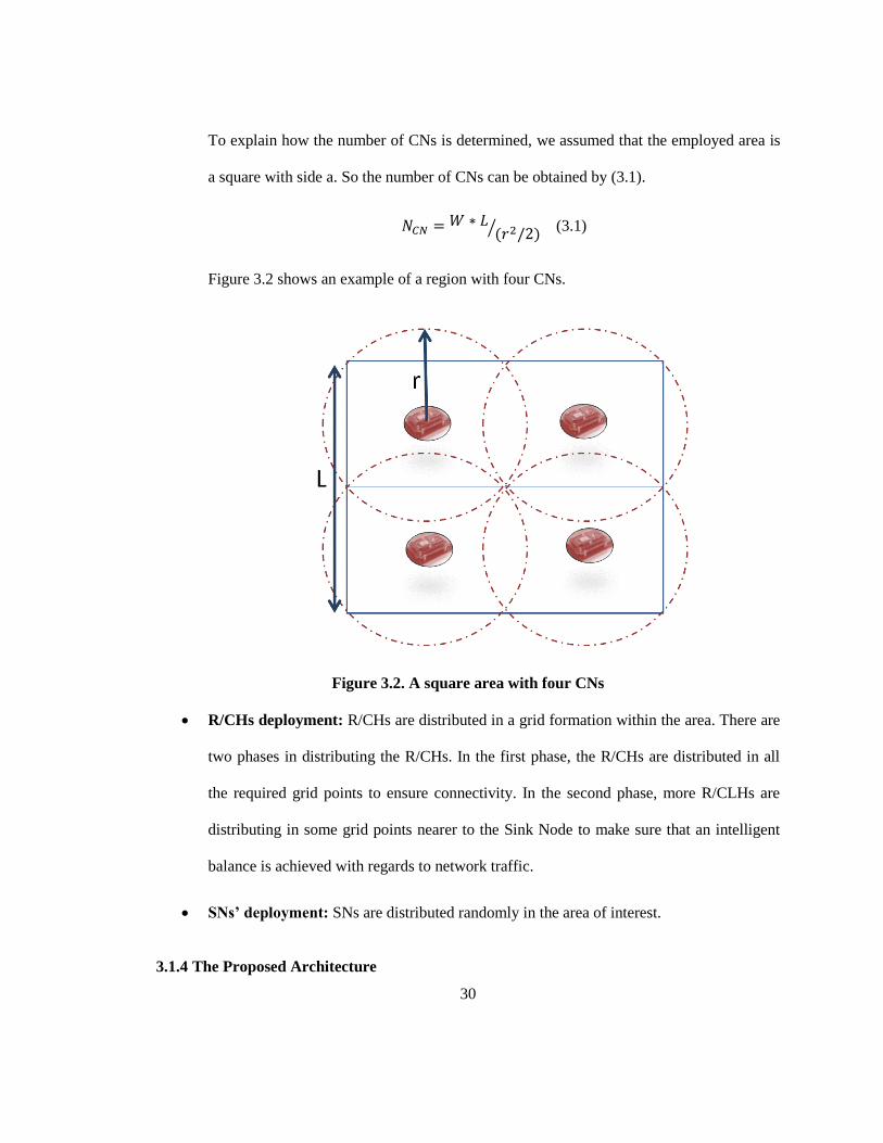
To explain how the number of CNs is determined, we assumed that the employed area is
a square with side a. So the number of CNs can be obtained by (3.1).
(3.1)
Figure 3.2 shows an example of a region with four CNs.
Figure 3.2. A square area with four CNs
R/CHs deployment: R/CHs are distributed in a grid formation within the area. There are
two phases in distributing the R/CHs. In the first phase, the R/CHs are distributed in all
the required grid points to ensure connectivity. In the second phase, more R/CLHs are
distributing in some grid points nearer to the Sink Node to make sure that an intelligent
balance is achieved with regards to network traffic.
SNs’ deployment: SNs are distributed randomly in the area of interest.
3.1.4 The Proposed Architecture
31
The architecture of the network is a multi-tier or hierarchical one. As shown in Figure 3.3, there
are four tiers in the network:
First Tier: this is the highest level in the network and contains the Sink Node and end
users. The Sink node is able to communicate with all nodes in the network. Thus, it can
send commands to all nodes to control them or to receive data from them. End users can
also communicate with all nodes by sending commands to the Sink Node.
Second Tier: the CNs belong in this layer. The communication among CNs and other
nodes in the network requires only one-hop. This one-hop communication reduces the
extra load of cognition. CNs are also able to receive commands from the Sink Node, and
make appropriate decisions. It is worth noting that the Sink Node can send commands to
SNs to change their Sensory Data Rate (SDR) or sleep/awake duration.
Third Tier: this tier comprises R/CHs. Each R/CH has several children and is
responsible for forwarding the data generated/collected by its children toward the Sink
Node as well as the data forwarded by other R/CHs. The R/CHs can communicate with
their children, other R/CHs, and upper layers’ nodes.
Fourth Tier: SNs make up this layer. Since SNs are RFDs, SNs cannot communicate
with each other. SNs can only send data to their parents (related R/CHs) and receive
commands from higher levels’ nodes and act accordingly.

32
Figure 3.3. The Multitier network
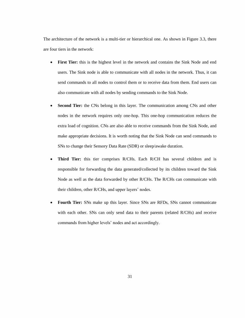
Figure 3.4 depicts the complete architecture of the system. As shown, there are several groups in
the network. Each group contains several SNs, several R/CHs, and a CN. Each CN is responsible
for managing the SNs and R/CHs in its confine. However, the CNs can communicate with each
other and send necessary commands to each other. The generated data is forwarded to the Sink
Node via R/CHs and the Base station forwards the data to the clients (end users) using GPRS via
the internet.
33
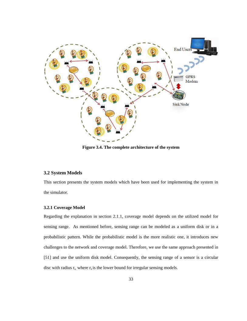
Figure 3.4. The complete architecture of the system
3.2 System Models
This section presents the system models which have been used for implementing the system in
the simulator.
3.2.1 Coverage Model
Regarding the explanation in section 2.1.1, coverage model depends on the utilized model for
sensing range. As mentioned before, sensing range can be modeled as a uniform disk or in a
probabilistic pattern. While the probabilistic model is the more realistic one, it introduces new
challenges to the network and coverage model. Therefore, we use the same approach presented in
[51] and use the uniform disk model. Consequently, the sensing range of a sensor is a circular
disc with radius rs, where rs is the lower bound for irregular sensing models.

34
In this thesis, we are trying to monitor a specific target points. Therefore, a target is covered by a
SN if its distance from that SN is less than rs.
3.2.2 Lifetime Model
One of the main goals of proposing different protocols and algorithms for WSNs is to extend the
network lifetime. As a result, being aware of the energy consumption model of the network is a
key factor for designing a protocol with a reasonable overall lifetime performance. Hence, in this
section, first, the energy model of a node in a WSN is investigated and then the definition of
lifetime in this thesis is provided.
3.2.2.1 Power Consumption Model
As mentioned before, aside from conducting our simulations, we are evaluating our proposal
through implementing the system with CC2530. Hence, the energy model presented in [33] is
used so as to achieve simulation results that are closest to the real node consumption patterns.
In order to calculate the power consumption, the voltage and current are needed.
(3.2)
The current should be calculated in two phases: 1) the current in active mode and 2) the current in
sleep mode. The average current can be calculated by accumulating the power consumption of the
two phases.
(3.3)
Where T is the period of transmitting packets.
The goal of this work is to design a network with full coverage and full connectivity while
prolonging the network’s lifetime. Sufficient R/CHs are distributed in the network to provide

35
connectivity. SNs are responsible to cover target points. Therefore, the network lifetime can be
defined as following:
Definition 1. (Lifetime Definition): Lifetime of a WSN is a time span from network deployment
until there is at least one uncovered target points.
3.2.3 Communication Model
Similar to coverage model, there are two types of communication model: a uniform disk and a
probabilistic model. We assume that the communication range is a uniform disk with radius rc.
However, since the wireless signals may affect by the surrounding environment, we need to
consider an appropriate propagation model. Therefore, we explain the adopted propagation model
for calculating the probability or receiving the transmitted signal in the next section.
3.2.3.1 Propagation Model
To predict the received signal power of each packet at the receiver side, the radio propagation
model should be implemented in the simulator. By using the propagation model, the receiver is
able to calculate the received power and to mark packets that their received power is less that the
configured threshold as error. The packets with power below the threshold will be dropped in the
MAC layer. One of the most common and realistic model for propagation in high transmission
range applications is the log-normal shadowing model which contains two main factors: path loss
and fading effects of the channel [34]. Thus, based on the log-normal shadowing model, the
signal level at distance “d” from a transmitter can be calculated by (3.4).
( ) ( ) 10 log( )0
0
dP d P P rsd loss r
(3.4)

36
Where Ps is the transmission power, Ploss(r0) is the path loss measured at reference distance r0
from the transmitter, β is an environment dependent path loss exponent, and χ is a normally
distributed random variable with zero mean and variance σ2, i.e. χ ~ N(0, σ
2).
As shown in [25], another important factor in is the value of packet retransmission in MAC layer.
When a node receives a packet correctly, it sends a MAC ACK to the transmitter. The transmitter
waits for a specific amount of time to receive the MAC ACK. If a MAC ACK is not received, the
packet is retransmitted. The farther the nodes are from each other, the more retransmissions are
required to generate a specific Packet Error Rate (PER). The maximum number of
retransmissions to have a specific PER is set based on the provided results in [25].
3.2.4 Network Model
The network is modeled as a graph ( , )G V E , Where 1 2{ , ,..., }NV n n n is the set of nodes
(except CNs) in the network, E is the set of edges (links) in the network, and ( , )i j E if at least
one of the in or jn is an R/CH and the Euclidean distance between them is less than their
minimum communication range.

37
Chapter 4
Cognitive Network Framework
In this chapter, we explain the proposed cognitive framework. First section provides an overview
of different states of a CWSN during its operation. The proposed cognitive management process
is explained in section 4.2. A Graphical User Interface (GUI) is designed to provide required
information about the network for users. The user can control the network parameters by using
the GUI. Details of designed GUI are explained in section 4.3.
4.1 System Overview
This thesis aims to enable cognition in WSNs. Based on our working definition of cognition the
network should:
1. Be aware of the current condition of the network, i.e. available nodes, their positions,
their available battery, and target points.
2. Be aware of the current user requirements and their priority.
3. Make appropriate decisions to satisfy the users as much as possible based on the available
resources.
Therefore, we propose that a cognitive management process should be embedded in the network
in order to enable cognition. The cognitive management process consists of three sub-processes:
scanning the network, decision making, and informing nodes from taken decisions. The cognitive
management process is completely explained in this section.
In a regular network, after forming the network (system initialization), the network will continue
to work based on the implemented protocols and algorithms (this is referred to as its working

38
state). However, in a CWSN, there is another state which is called the cognitive management
process. Therefore, a CWSN has three states:
1. System initialization: the system, by default, starts from this state. In this state, the
network is being constructed. The nodes are joining the network, all the required tables,
such as routing tables, are constructed, and other required system initializations are done.
2. Cognitive network management: in this state all the required decisions are taken and will
be sent to the related nodes.
3. Working state: in this state, the network functions based on the scheduling assigned to the
nodes during the cognitive network management state. The cognitive process section of
the cognitive network management determines the duration of the working state.
A system transition diagram is depicted in Figure 4.1, while Figure 4.2 shows the states during
lifetime of the network.
Figure 4.1. System transition diagram

39
Figure 4.2. Network states
As it is shown, the network periodically transitions between the three states. However, in order to
achieve an acceptable performance, the duration of the steady state should be longer than the
network management duration. Therefore, mT T should hold in the network.
As mentioned before, to implement the network management process in the network a new node,
named Cognitive Node (CN), is introduced to the network. The CN is responsible for creating
profile tables for the nodes within its confine so as to keep track of their status as well as make
decisions and update nodes about taken decisions. The CN will run the cognitive management
process iteratively. To decrease the complexity, we assume that the maximum number of
iterations is R and the current round will be shown by r.
4.2 Cognitive Network Management Process
This section explains the cognitive network management process. The objective of the process is
to enable cognition (with concept of awareness, learning, reasoning and decision making) in
WSNs. To this end, it contains at least three sub-processes:
1- Scanning the network: The purpose of this process is to provide awareness for the
decision-making process. Simply put, it means providing the required information about
the network’s current condition, nodes’ statuses, and user requirements. To achieve this
goal, it creates a profile table for each node and each target in the network, and updates
the tables regularly in order to remain cognizant of any changes.

40
2- Decision-making: The goal of this process is to make appropriate decisions based on the
current network situation. Decisions can be about different aspects of the network such as
node activity modes (active or sleep), Frequency of Sensing (FoS), route to the
destination (routing layer), and medium access (MAC layer). The process uses the data
from the profile tables that are provided by the scanning the network process.
3- Updating the nodes from taken decisions: This process aims to transmit the decisions
taken by the decision-making process to the related nodes. The decisions can be
transmitted as MAC layer control messages.
The remainder of this section presents the proposed algorithms for each of the above processes.
4.2.1 Scanning the Network
One of the first issues in a CWSN is how to provide information about current network conditions
and user requirements. To this end, in our proposal a profile table with appropriate fields (the
fields can be specified based on the information required through the decision-making process)
has to be constructed for each node as well as the target points. As the Cognitive management
process is implemented in the CNs, CNs are responsible for executing the processes that belongs
to cognition. The first step for each CNs is to recognize the nodes and targets within its purview,
and to be able to create the profile tables as well as perform the decision-making processes. The
following steps describe the recognition-process of CNs:
1) Each CN sends a message advertising its ID and its purview (the geographical
information of the area that the CN is covering).
2) The nodes that receive this message and are in the specified region send a join message to
their relative CN. Based on the employed algorithm for node management, the join

41
message may contain information about nodes’ positions, available battery levels, and
etc.
3) Each CN creates a profile table for the nodes that are in its purview and sends a join
request. Profile tables update repeatedly to maintain awareness about the current network
conditions and nodes’ statuses. In addition to the nodes’ profile table, a profile table is
constructed for each target. The targets’ profile table can be uploaded on CNs before the
network deployment or during the network initialization state by the Sink Node.
The recognition-process will be operated only once for each CN. After identifying the nodes and
targets for which a CN is responsible, the CN will keep the information about the nodes and
targets in the constructed profile tables and update the tables by using the update information
transmitted by nodes after each working state (refer to Figure 4.1). In the following, different
fields within profile tables of SNs, R/CLHs, and targets are presented.
4.2.1.1 SNs’ Profile Table
The profile table contains the position of SNs, their Battery Level (BL), Utility Factor (UF),
Service ID, Frequency of Sensing (FoS), Packet Loss Ratio (PLR), and Link Throughput.
BL: Critical points in the discharge characteristic figure of the battery are determined as
different battery levels. Critical points are the points at which the speed of the battery
deterioration changes significantly (more details on section 4.2.2.2).
UF: By this factor the CN determines the importance of the sensors and of the
information. A higher UF means that more information is needed and the related SNs
must send data at a higher rate. UF of a SN can be determined from the importance level
of the targets that the SN covers or can be specified directly by the user.

42
Service ID: Since we have different kinds of sensors in our network, each one has a
Service ID (e.g. SID = 1 means that the attached sensor is a temperature sensor and SID =
2 means that the attached sensor is a camera sensor). Each sensor has its individual
characteristics.
Available Buffer: It shows the available buffer in the SN.
RN: This number is the ID of the parent (the related R/CH) of the SN.
PLR: It shows the number of dropped packets at the related R/CH to the number of
generated packets at the SN.
Link Throughput: Shows the average throughput of the current link between the SN and
the related R/CH. It is calculated by dividing the number of successfully transmitted
packets by the duration of time that the node worked in the active mode.
A sample table is shown in Table 4.1.
Table 4.1. SNs’ profile table
SN
position
Remaining
Battery
UF FoS Service
ID
Available
Buffer
RN PLR Link
Through.
{ x1 , y1 } Ks1 UFs1 FoSs1 SIDi1
Qs1 RNs1 PLRs12 LTs1
3
… ….. … … … … … … …
{ xsN , ysN
}4
KsN UFsN FoSsN SIDi Qs2 RNsN PLRsN LTsN
4.2.1.2 R/CHs’ Profile Table
1 1 i l which l is the number of the different kinds of sensors
2 0 1PLR
3 0 1LT
4 N is the number of SNs

43
Each R/CH has a profile table that contains the position of the R/CH, the remaining battery, the
number of children, the available buffer, and the available Flow.
Table 4.2. R/CHs’ Profile Table
R/CH position Remaining
Battery
Number of
the Children
Available
Buffer
Flow Rate
{ xr1 , yr1 } Kr1 Chr1 Qr1 FLr1 pps
… ….. … … …
{ xrZ , yrZ }5 KrZ ChrZ QrZ FLrZ pps
4.2.1.3 Targets’ Profile Table
There is a table for each target constructed by CNs in order to keep track of the targets’ current
status and requirements. The table contains the position of targets, the targets’ importance level,
and required services for the targets. Table 4.3 shows a sample of a targets’ profile table.
Table 4.3. Targets’ profile table
Target position Importance Level Required Services
{ xt1 , yt1 } ILt1 RSet16
… … …
{ xtM , ytM7 } ILtM RSetM
4.2.1.4 CNs’ Profile Table
Each CN has a profile table which contains the position of the CN, the available battery, the
number of targets in the CN span and their ID, and the number of SNs assigned to the CN. Table
4.4 shows a sample table with different fields.
5 Z is the number of R/CHs
6 RSeti is a list of required services by target i, e.g. RSet2 = {SID1, SID4}
7 M is the number of the targets

44
Table 4.4. CNs’ profile table
CN position Remaining Battery Targets Number of SNs
{ x , y }
KCNi {TCNi, Tar18, Tar2,
Tar6, … , Tari}
NCNi
4.2.2 Decision-making Process
As previously mentioned, the ultimate goal of a CWSN is to dynamically adapt itself to the
environment in order to improve network performance while considering user requirements. In
this thesis our focus is to manage the SNs’ activities. Consequently, we aim to determine the FoS,
the status of the SN (active or sleep), and the duration of activity in each specified mode.
Different challenges of organizing a WSN should be considered in order to improve network
performance and satisfy users. Among different expressed criteria for WSNs, network lifetime,
connectivity, and coverage are essential. Therefore we consider lifetime, connectivity, and
coverage as primary optimization criteria. Connectivity is addressed by distributing enough
R/CHs in the area of interest. Thus, we are aiming to maximize network longevity while
maintaining coverage in the network. Several algorithms are proposed in the literature to solve
the problems of maximizing network longevity while maintaining coverage in the network [7]-
[9]. Amongst the proposed algorithms, we have used the proposals in [7] as our reference. The
authors in [7] improved network lifetime by dividing SNs into a number of sets. Each set must
completely cover all targets. Therefore, at any given time a given set of SNs must be in active
state (sense, receive, and transmit) and all others must be in sleep state. Thus, the network
lifetime is improved by avoiding redundant data while full coverage is achieved. The advantages
of the proposed algorithm in [7] are as follows: 1) the constructed sets are not disjointed and a SN
can be activated in different sets. Consequently, active duration of each cover set decreases and
8 Tari is the ID of target i
…Nt…

45
the network may have higher tolerance to node failure, 2) the authors solved this problem by two
heuristic algorithms. One of the heuristic algorithms, the Greedy algorithm, has low complexity
and is implementable. However, the authors assumed that the network is homogeneous. In
addition, changes in the network conditions have not been considered. Therefore, the SNs’
schedule is static and doesn’t change during the network operation.
In [35], the authors proposed an algorithm to prolong network longevity while maintaining
coverage and connectivity for heterogeneous WSNs The authors showed that using a
homogeneous model for a heterogeneous network causes energy waste in the network and it is
necessary to have a model that is uniquely constructed to serve heterogeneous networks.
However, as the authors mentioned, the complexity of their model is high and is not
implementable. Thus, in this thesis, we addressed heterogeneity while considering complexity of
the algorithm.
4.2.2.1 Problem Statement and Contribution
Similar to [7]:
The goal is to schedule the activity of “N” SNs distributed in the area of interest to continuously
cover “T” target points while the network longevity is maximized.
However, in contrast with traditional scheduling algorithms (and also [7]):
1- N SNs are not homogenous,
2- Each Target can request information for more than one unique sensory genre,
3- The FoS is one of the variables that should be determined based on the network’s current
condition,
Therefore, the contribution of our algorithm necessarily addresses:
1- The issue of heterogeneity while the program is computationally feasible to solve,

46
2- Awareness of network condition and adaptability,
3- Determining the Frequency of Sensing (FoS) as well as duration of staying in active/sleep
mode,
4- A consideration of other criteria in the network, such as flow, throughput, and PLR, for
scheduling SNs.
The scheduling process is divided into two processes: one for determining the FoS, and the other
for determining the working mode (active or sleep) as well as duration of staying in the
determined mode.
4.2.2.2 Determining Frequency of Sensing (FoS)
Frequency of Sensing (FoS) can be determined based on the current condition of the network as
well as the user requirements. We propose to create a reference table that contains the appropriate
FoS for different cases, and upload it on CNs. Therefore, CNs can determine the value of FoS
using the SNs’ profile table and the reference table. To create the reference table, two factors will
be used; the Utility Factor (UF) and the Battery Level (BL) of SNs.
UF shows to what degree the information provided by a particular SN is important to the user.
Since SNs send their data periodically to the base station, more UF means that more data has to
be sent. UF can be set directly by the user or can be determined by CNs. CNs use the target
importance level to determine the UF. As each SN may cover more than one target, the highest
level of importance among effective targets is the one that is used to determine the UF. In our
network, we assumed that the UF and importance level have a direct relation. Thus, if a SN
covers targets with importance levels of 3, 2, and 1, the UF would match the highest importance
level, i. e. 3.

47
There is a different range for FoS for each level of UF; [ FoSmin , FoSmax ]. Users can specify the
range based on the requirements at each level of target importance since the UF and importance
levels are directly connected.
BL is obtained from the Discharge Characteristics of the battery that we are using. In our
experiments we will use the Energizer NH15-2300. The discharge characteristic is shown in
Figure 4.3.
Figure 4.3. Discharge characteristics of the used battery
The goal is that FoS follows the battery reduction pattern to increase the lifetime of the network.
This is made possible by mapping the FoS range to the discharge characteristic fucntion. The
mapping is shown in Figure 4.4.
Figure 4.4. Mapping the FoS range to the discharge characteristic diagram

48
In this case, the FoS changes smoothly by changing the BL. The forced load of cognition,
however, is too/very high. This is because of the high amount of required messages and memory.
To reduce the load, the FoS changes just at certain BLs or critical points in the discharge
characteristic function. Critical points are the points at which the speed of battery deterioration
(slope of the figure) is changing significantly. The chosen critical points (BL) for our experiment
are shown in Figure 4.5. While Figure 4.6 depicts the relationship between FoS and BL.
Figure 4.5. Critical points
Figure 4.6. Relationship between FoS and BL

49
We have 5 levels of importance leading to 5 levels for UF. By having the FoS for each level of
UF, we are able to construct the FoS table. As the network contains different kinds of SNs, it may
have different FoS ranges in different levels. Therefore, we first categorized SNs based on
different applications and their requirements. We assumed that we have two different applications
and different tables for different applications. Table 4.5 shows the table that we used in our
experiment.
Table 4.5. FoS table used in the experiment
UF \ BL S1 S2 S3 S4 S5
UF1 0.033333 0.032937 0.0327948 0.0325397 0.016667
UF2 0.008333 0.008234 0.0081987 0.0081349 0.004167
UF3 0.002083 0.002059 0.0020497 0.0020337 0.001042
UF4 0.000833 0.000827 0.0008244 0.0008201 0.000556
UF5 0.000277 0.000274 0.0002733 0.0002712 0.000139
FoS table for the first application
UF \ BL S1 S2 S3 S4 S5
UF1 0.003333 0.003294 0.003279 0.003254 0.001667
UF2 0.001111 0.001098 0.001093 0.001085 0.000556
UF3 0.000556 0.000549 0.000547 0.000542 0.000278
UF4 0.000139 0.000138 0.000137 0.000137 9.259259
UF5 9.259259 9.171076 9.139582 9.082892 5.555556
FoS table for the second application

50
4.2.2.3 Maximum Set Cover (MSC) Problem Definition and Formulization
To determine the activity mode of SNs and their duration, an MSC problem is defined and
formulated in this section. We use the same definition provided by Cardee et al. in [7]. However,
for formulating the problem we use linear programming pattern instead of the integer
programming one.
We explain the problem by using an example. Figure 4.7, depicts an example of a network with 5
SNs and 3 target points along with the coverage area of SNs, while Figure 4.8 provides two
possible cover sets.
Figure 4.7. A sample of the network with 5 SNs and 3 target points

51
Figure 4.8. Two possible cover sets
As illustrated in the above figures, the sets are not disjoint and an SN can be in more than one
cover set which is better than the disjoint cover sets based on the explanation in reference [7]. The
duration of each set cover depends on the current available battery of the SNs. As explained in
4.1, CNs perform cognitive algorithms iteratively and each round has a number “r”. The
maximum number of rounds is predefined and is “R”. Therefore, CNs will consider a portion of
actual available battery level as the current available energy for the current round. The available
energy of each SN for current round will be calculated using the following equation:
for all (4.1)
Therefore, we define the problem as the following:
MSC Problem Definition
Given a collection of SNs si and target points TarM, find a group of set covers
SC1, …, SCp with time duration t1, …, tp in [tjmin,tjmax] such that to maximize t1 +…+ tp. And for
each subset Si in SNs, si appears in SC1, … , SCp with total weight of at most , where is the
current available battery capacity of each SN.

52
Linear Programming MSC Problem Formulization
In order to formulize the problem, we first need to list available parameters as well as variables. It
is essential to remark that all SNs, R/CHs, and targets have a profile table containing the
information about current status of them. We use the required information obtained from profile
tables for our optimization.
Given:
p is the bound for the number of set covers,
{SN} = {s1, s2, … , sN} is a set of “N” SNs,
sik for si{SN} which is the current available energy of si,
FOSsi for si{SN} which is the current FoS of si,
Qsi for si{SN} which is the current available buffer of si,
l
sie for si{SN} which is the energy consumption pattern of si with offering service “l”,
{TAR} = {tar1, tar2, … , tarM} is a set of “M” targets,
{R/CH} = {R/CH1, R/CH2, …, R/CHZ} is a set of “Z” R/CHs,
FLR/CH is the available output flow of R/CH,
QR/CHi for R/CHi{R/CH} which is the current available buffer of si,
C = [cki]M×N is a matrix of the relationship between targets and SNs; where cki = {1| if
target tark is covered by si and the services offered by si are in the required service list of
tark},

53
Ck = [ck1 ck2 … ckn]1×n for k = 1, … , M ; Ck is kth row of C,
Variables:
tj for j = 1, … , p to represent the time allocated for the set cover Sj and is bounded by the
lifetime of the node which is subject to ran out of energy faster compared to all other
nodes in the set cover j.
X = [xij]N×p where xij = {1| if SN si is in the set cover Sj} to represent if a node is active in
time duration of tj,
Xj =[x1j x2j … xNj]1×p is jth row of X.
The goal is to maximize the network lifetime which can be formulated as the summation of
assigned duration to the set covers:
(4.2)
While maintaining the network coverage (there is at least one SN covering each target):
for j=1,…,p (4.3)
Where XjT is the transpose of Xj.
And also manage the network based on the current available energy in the SNs:
for all (4.4)
Where iEC is the Energy Consumption of si and is calculated by:
for all (4.5)
By applying (4.5) in (4.4), (4.4) can be written as:

54
(4.6)
To convert the problem to the form of linear programming, we set
(4.7)
Therefore, (4.3) and (4.6) can be rewritten as following:
for all (4.8)
for all (4.9)
A relaxation technique is applied to be able to solve the problem:
(4.10)
Where maxjt is the maximum possible duration for a set cover and
minjt is the minimum duration
of a set cover. The rationale behind having the boundary for tj is that the goal is to have full
coverage.
The values are calculated by using following formula:
for all (4.11)
for all (4.12)
We considered available bandwidth in the network as another criterion to prevent overflow in the
network. In general following equation can be written for each node in the network:
for all nodes (4.13)

55
Where FLo is the output flow, FLi is the input flow, G is packet generation rate, Q is the available
buffer, and T is the duration of time. T should be equal to tjmax in order to prevent overflow (tjmax
is the worst case).In our system, R/CHs don’t generate any packet:
for all (4.14)
And for SNs:
for all (4.15)
for all (4.16)
Therefore, the overflow constraint should be written only for R/CHs.
for all (4.17)
Where FLR/CH is the available output flow in the profile table of R/CH.
By using the above explanation the optimization problem can be written as:
Subject to for all
for all
for all

56
The problem is solved by two heuristic solutions: 1- Linear Programming (LP) algorithm, and 2-
Greedy algorithm. However, the additional factors defined in our problem formulization should
be considered. In the following two proposed solutions are explained.
4.2.2.4 Linear Programming Solution
As mentioned before, the goal is to improve the network performance. One of the first and
important optimization goals is to prolong lifetime. We are seeking this goal by removing
redundancy. Thus, we first solve the linear programming formulated in previous section and
nominate a series of SNs to cover target points. Then, algorithm removes the redundancy while
considering all the optimization objectives (e.g. PLR and throughput) by selecting the best SNs
among the nominated SNs. The best sensor will be chosen based on the priority calculated by
following equation:
for all (4.18)
Where i is the coefficient of each parameter and can be set by CNS, PLRsi is the PLR in the
profile table of si, and LTsi is the link throughput in the profile table.
The algorithm takes {SN} (the set of SNs and their profile table), {TAR} (the set of target and
their profile table), {R/CH} (the set of R/CHs and their profile table), p and returns ‘n’ (number
of created set cover), the SC1, SC2, …, SCn (set covers), and the t1, t2,…,tn (duration of set
covers).
Linear Programming Algorithm: creating Set Covers
1: Function Create_Set-Covers
2: Input:
3: R, r, p, SN, R/CH, TAR
4: Output:
5: n, SC1, SC2, …, SCn

57
6: Begin:
7: forall si {SN} do
8: k′si = ksi / (R-r); /* ksi is the available energy in profile table of SNs */
9: endfor
10: n = 0;
11: while each target can be covered by at least one SN do
/* a new set cover Cp will be formed */
12: Execute the LP using the MATLAB toolbox;
13: * *( , )ij jy t for i=1,…,N and j=1,…,p is the output of the LP;
14: forall j=1 to p do
15: set 0ijy for all si {SN};
16: set for k = 1,…,M;
17: forall k= 1 to M do
18: for si Ck with *
ij jy t do
19: Calculate the “priosi” using (4.18);
20: Choose the si with highest “priosi” and set ij jy t ;
21: SCj = SCj si;
22: endfor
23: endfor
24: endfor
25: forall si {SN} do
26: ksi = ksi - ( )i jEC ;
27: /* ( )i jEC is calculated by (4.5) */
28: if ksi == 0 do
29: {SN} = {SN} – si;
30: endif
31: endfor
32: n = n + p;
33: endwhile
34: return n, (SC1, SC2, …, SCn), (t1,…,tn)
35: End
In line 7-9, the algorithm calculates the current available energy based on the remained energy in
SN’s profile table as well as the current round. After finding solution by executing the LP in lines
12-13, the algorithm removes redundancy and constructs set covers in lines 14-24. In lines 25-31,
the remaining energy is calculated. Then if based on the remaining energy all the targets can be
covered, the algorithm will go to the line 12 and starts to solve the LP problem again and

58
construct new set covers based on the remaining energy. Therefore, the algorithm iterates until
there is at least one uncovered target.
For analyzing the runtime complexity of the program, we divided it into three parts: LP parts,
lines 14-24, and lines 25-31 and consider the M (number of targets), N (number of SNs), and p
(number of set covers) as the parameters. Based on [52], the runtime of LP is Q(K3) where K is
the number of parameters. Therefore the runtime of LP in our algorithm is O(p3(N+1)
3). The
runtime of lines 14-24 is O(MNp) and the runtime of third part is O(N). Since M N, the
runtime of LP nominated the runtime of other two parts and therefore, the runtime of the
algorithm is O(N3p
3).
The pseudo-code and flow chart of implemented algorithm is provided in Apendix A.
4.2.2.5 Greedy Solution
In order to have an algorithm which is computationally feasible to solve and implementable, we
proposed a greedy algorithm. The objective of the algorithm is to create the highest possible
number of set covers in order to maximize the lifetime of the network.
Analogous to presented algorithm in reference [7] our algorithm sets the duration of each set
cover as ‘w’ before execution. Both algorithms sort the targets based on their criticality level and
choose the SN with the greatest contribution for covering each target. However, our criteria for
setting the criticality level of target and contribution of SNs is different with [7].
In our proposal, the criticality level of targets will be determined based on the three factors: 1)
importance level set by user, 2) available energy in the battery of the SNs covering the target, 3)
available flow in the R/CHs which are the parents of the SNs covering the related target. For
determining the contribution of each SN, a priority formula presented in (4.19) is used:
for all (4.19)

59
Where i is the coefficient of each parameter and can be set by CNs, PLRsi is the PLR in the
profile table of si, LTsi is the link throughput in the profile table, and T
siN is the number of targets
that SN si covers.
The algorithm takes {SN} (the set of SNs and their profile table), {TAR} (the set of target and
their profile table), {R/CH} (the set of R/CHs and their profile table), and w (the duration of each
set cover) and returns ‘n’ (number of created set cover), the SC1, SC2, …, SCn (set covers).
Greedy Algorithm: creating Set Covers
1: Function Create_Set-Covers
2: Input:
3: R, r, {SN}, {R/CH}, {TAR}, w
4: Output:
5: n, SC1, SC2, …, SCn
6: Begin:
7: forall si {SN} do
8: k′si = ksi / (R-r); /* ksi is the available energy in profile table of each SN */
9: endfor
10: n = 0;
11: while each target can be covered by at least one SN do
/* a new set cover Cp will be formed */
12: n = n + 1;
13: Cn = Ø;
14: Targets = TAR;
15: While Targets ≠ Ø do
16: Find a critical target Targets
17: Calculate the “prio” using (4.19)
18: Select the si SN with highest “prio”
19: Cn = Cn si;
20: forall targets tar Targets do
21: if taru is covered by si do
22: Targets = targets – taru;
23: endif
24: endfor
25: endwhile
26: forall si {SN} do
27: l
si si i ik k FoS w e ;
28: if ksi == 0 do
29: {SN} = {SN} – si;
30: endif

60
31: endfor
32: endwhile
33: return n, (SC1, SC2, …, SCn)
34: End
Similar to the LP algorithm, the greedy algorithm calculates the current energy for this round
based on the current available energy in the SNs’ profile table in lines 7-9. In lines 15-25, the
algorithm constructs a set cover. The redundancy is removed in lines 20-24 by removing the
targets which are already covered by chosen SNs for set cover. Lines 26-31 calculates the
remaining energy and algorithm will back to line 12 in order to start constructing a new set cover
if all targets can be covered based on the remaining energy.
The runtime of greedy algorithm is O(nM2N) where n is the number of set cover, M is the number
of targets and N is the number of SN.
The pseudo-code and flow chart of implemented algorithm is provided in Apendix B.
4.2.3 Updating the Nodes from Taken Decisions
This algorithm is responsible for informing nodes of decisions regarding nodes’ working state
(sleep or active), duration of working in this state, and assigned FoS (which is taken by the
decision making algorithm). This information can be transmitted by using extra control messages
or by embedding it in the MAC packets. In this thesis, we release this information through MAC
frames.
4.3 Graphical User Interface for WSN
The goal of the Graphical User Interface (GUI) program is to provide information about the
current condition of the network to end-users as well as the ability to change the parameters (such

61
as FoS) of the network. Therefore, in addition of having cognition by using CNs, users can
manually change the status of nodes by using the designed GUI.
The program shows the battery level, sensing information, and GPS information (if it is available)
to the user. To help users have a vision about the previous working states in the network, the
program provides a figure about energy dissipation of the nodes. The disadvantage of the
program is that it is completely dependent on the information provided by SNs gathered by R/CH
and sent to the FTP server by GPRS. Therefore, if an R/CH dies, the program will lose the
information about the end devices which belonged to that R/CH until SNs can find another R/CH,
if there is any available in their range.
A snapshot of the program is shown in Figure 4.9.
Figure 4.9. A snapshot of the GUI program
Different parts of the designed GUI program will be explained in the following. As you can see in
the provided snapshot, the Program consists of three main parts:

62
1. File Transfer Protocol (FTP) section: The program connects to the FTP server and gets
the updated information which is regularly provided by SNs. In order to connect to the
FTP server, the user should enter the required information in the FTP connection section.
This information consists of: the FTP server name, the File name in FTP (File should be
in the main directory), the User name and, the Password to access the FTP. By pressing
the connect button, the GUI will connect to the FTP server using the provided
information. The status of the connection is shown in the connection status section:
“FTP connected” which means there is no problem in the connection
“FTP connected busy” which means the GUI is already connected to the FTP
server and is busy reading the file and updating the tables and graphs.
“There is a problem in the FTP connection” which means the username or
password of ftp connection is not true.
“There isn’t such file” which means the GUI couldn’t find the file in the FTP
server.
The program, then, extracts the useful data from the stored information, updates the table
and figures. Therefore, it is important to know about the format of the data in order to
extract useful data. The file format that this program accepts is as following (every
information line follows by a line which indicates the time of reporting the information):
‘D’ ‘application node ID’ ‘battery level’ ‘temperature’ ‘other measurements’
‘d/m/y’ ‘h:m:s, time zone’
‘G’ ‘‘application node ID’ ‘latitude’ ‘longitude’ ‘time’

63
‘d/m/y’ ‘h:m:s, time zone’
2. SN section: User can have more details about each SN by entering the SN ID number
and pressing the show button. User has the first and last report time, the last reported
battery level, the GPS information (if the sensor has a GPS), the sensory measurement
value (now only temperature), and also a plot that shows the energy consumption pattern
of the SN.
3. Overview section: In the overview section, last reported battery level of all nodes and
last update time (day and time) is shown.
In the ‘Num. of Nodes’ and ‘Update Period’ sections, user can enter the number of nodes in the
network as well as the updating period.

64
Chapter 5
Performance Evaluation
In this chapter, the proposed cognitive architecture is evaluated by both simulation and
implementation. The rationale behind implementation is that since most of the previous works
have been done in simulation, there is a need to explore implementation issues and consider them
while designing a new protocol or algorithm. We also evaluated the system by designing a
simulator in MATLAB to be able to analyze the system behavior in large scales. The proposed
CWSN is evaluated by comparing the performance of a CWSN with improved-MINA protocol,
presented in [24], in terms of lifetime, scalability, throughput, Packet Loss Ratio (PLR), and
runtime complexity of algorithms. The employed architecture for improved-MINA is a multilayer
architecture without any cognition layer. The MAC and routing protocols are the same in both
networks and the management in the improved-MINA network should be done by Sink Node at
the first moment of the network deployment. Both networks were tested under identical
conditions in different scenarios. Different scenarios were chosen to test how both protocols
perform under different conditions and to explore advantages and disadvantages of our proposal.
The chapter is organized as following: after presenting the simulation setup and evaluation
parameters in sections 6.1 and 6.2, section 6.3 provides the simulation results as well as related
discussions. Section 6.4 describes the implementation setups, the employed hardware and
software, and the experimental results.
5.1 Simulation Setup
We simulated a stationary network with SNs and target points randomly distributed in the area of
interest. Our network contains four different types of sensors: camera, temperature, humidity, and

65
infrared. Each SN has one sensor, randomly chosen from the list of available sensors. Based on
available sensors, four different services are available in the network. Therefore, each target
points can have from one service and up to four services in its required service list.
The number of R/CHs will be determined based on the size of the chosen area in order to have
complete connectivity. Thus, the minimum number of R/CHs is calculated by (5.1):
(5.1)
Where w is width and l is length of the area, and rR/CH is the communication range of R/CH. The
R/CHs are distributed on grid points to make sure the area is fully covered and each SN can
access to at least one R/CH as its parent.
Additional R/CHs are distributed in the network if the number of children in R/CHs exceeds from
the threshold (we have limited bandwidth and based on the maximum flow of each link each
R/CH can support a specific number of links).
As it is explained in chapter 3, the number of CNs depends only on the area size and they will be
distributed in a grid to cover the whole area.
It is assumed that SNs, CNs, and R/CHs have different communication ranges. Communication
range depends on transmitter and receiver characteristics. Table 5.1, Table 5.2 and Table 5.3 list
the different parameters and their values in the simulation. Figure 5.1 depicts the nodes
arrangement in a part of the employed area.

66
Figure 5.1. Nodes’ arrangement in the simulator
Table 5.1. Simulation parameters – area and number of nodes
Parameter Value
Area size 100*250
Number of SNs 50~170
Number of Target Points 15
Table 5.2. Simulation parameters – communication and sensing ranges
Parameter Value Parameter Value
R/CLH com. range 100 Sensing range –
camera
40
CN com. range 250/2 Sensing range –
temperature
40
SNs com. range to
R/CLH
50 Sensing range –
humidity
45
SNs com. range to
CNs
100 Sensing range –
infrared
50

67
Table 5.3. Simulation parameters – physical parameters
Parameters Value Parameters Value
r0 5 m σ
10
Β 4.8 Frequency 2.4 GHz
Ps_CN 0 dB Pmin_CN 19 dB
Ps -117 dB Pmin -112 dB
Implemented routing and MAC protocols are the same as the presented ones in reference [24]
with required modifications for implementing the cognition.
5.2 Evaluation Metrics
We consider different metrics for evaluating the proposed system. The definition of each
parameter and the rationale behind choosing these parameters are explained in the following
sections.
5.2.1 Network’s Lifetime
Since one of the most important objectives in WSN is lifetime, we use network lifetime to
evaluate the efficiency of our proposed system. The goal of this work is to design a network with
full coverage and full connectivity while prolonging the network’s lifetime. Sufficient R/CHs are
distributed in the network to provide connectivity. Therefore, we use definition 1 provided in
section 3.2.2.
5.2.2 Runtime Complexity of Algorithms
As CNs schedule the activities of SNs repeatedly, the complexity of the cognitive algorithm is
important especially in real time applications. The run time is the maximum time that a CN needs
to manage the network at each round.

68
5.2.3 Throughput and Packet Loss Ratio
By using these two parameters we can evaluate the reliability of our system.
Throughput: Number of successfully received packet / Network’s Lifetime
[Packet/Second].
PLR: Number of lost packets / Number of generated and transmitted packets.
5.2.4 Battery Distribution
Having the even distribution of battery between the SNs can improve the network’s longevity by
decreasing the probability of losing coverage on target points. Therefore, we are using this
parameter to evaluate the load balancing feature of our proposal.
5.2.5 Different Simulation Scenarios and Results
We designed three scenarios to test different aspects of our system. In this section these scenarios,
related results, and explanations are presented.
First scenario:
The primary agenda of this scenario is to explore how awareness of network condition and
adaptation to new condition and requirements can improve the network performance (here
network lifetime). We compared the simplified version of cognitive network with the improved-
MINA network.
Improved-MINA Network: The MINA network is presented in reference [24]. To fairly
compare this network to our proposal we made some modifications in the proposed
architecture in order to improve the awareness level in the network. The modification
should also be done since heterogeneity is not addressed in reference [24]. The improved-
MINA network is a network with the same architecture as a CWSN but lacks cognition.

69
Thus, it has three layers for SNs, R/CHs, and Sink Nodes. The Sink Node commands all
the network management algorithms including the routing, MAC, and scheduling
algorithms. The FoS of the SNs should be determined and assigned to SNs by the Sink
Node before the network is deployed. The assigned FoS remains fixed during the
operation of the network.
Simplified-CWSN: The proposed CWSN is aware of the network condition and makes
decisions based on different criteria. This simple version of CWSN uses only the
information provided by/held within the physical and application layers, not all the layers
(MAC and routing layers). Thus, it will schedule the nodes’ activity solely based on the
available battery and user requirements.
Figure 5.2 compares network lifetime for all four algorithms. Following is the employed name for
different algorithms in the graphs: modified-MINA: LP-MSC and Greedy-MSC, Simplified-
CWSN: CLP-MSC and CGreedy-MSC.

70
Figure 5.2. Network’s lifetime
Based on the above figures, enabling cognition within the network improves its longevity. This is
the result of the awareness of the nodes’ status provided by the cognitive algorithm of the
network. However, for higher SNs, the Greedy-MSC algorithm has a superior longevity when
compared to CLP-MSC. This is because the Greedy-MSC receives information about the network
conditions by sorting the targets based on their criticality level and the SNs based on their
contributions. In addition, the greedy algorithm inherently avoids redundancy. Both reasons
position the greedy solution closest to an optimal solution.
By increasing the number of available SNs, we increase the options of choosing a SN for
covering a given target and consequently all algorithms show a better behavior. The improved
longevity by the CGreedy-MSC as compared to the CLP-MSC algorithm proves that the greedy
algorithm manages the network more carefully. Another important point to mention is that
although the network’s lifetime increases by increasing the number of SNs, the speed of this
increase eventually decreases. The reason is that by increasing the number of nodes, the

71
probability of nodes being in idle/sleep mode and the duration of staying in idle/sleep mode
increases. This cumulative energy consumption is unavoidable and can affect the network’s
longevity. Our research illustrates that idle/sleep mode energy consumption prevents a linear
increasing of the network’s longevity when the number of SNs is simultaneously increased.
As previously mentioned, network lifetime increases when cognition is enabled within the
network. To investigate the reason of such an improvement further, the average and standard
deviation of the remaining battery of the SNs is plotted in the following graphs.
Figure 5.3. Mean of the distribution of remaining battery of SNs
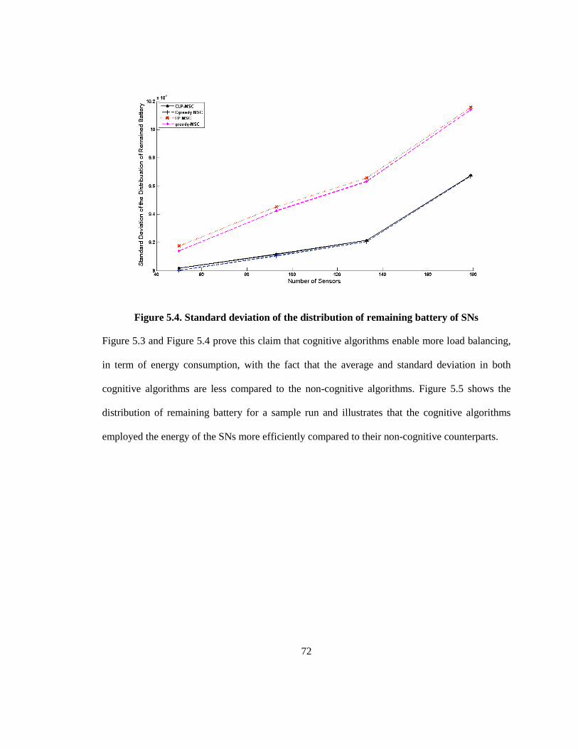
72
Figure 5.4. Standard deviation of the distribution of remaining battery of SNs
Figure 5.3 and Figure 5.4 prove this claim that cognitive algorithms enable more load balancing,
in term of energy consumption, with the fact that the average and standard deviation in both
cognitive algorithms are less compared to the non-cognitive algorithms. Figure 5.5 shows the
distribution of remaining battery for a sample run and illustrates that the cognitive algorithms
employed the energy of the SNs more efficiently compared to their non-cognitive counterparts.

73
Figure 5.5. Distribution of remaining battery
Figure 5.6. Network management runtime

74
Figure 5.7. Runtime for Cgreedy-MSC and greedy-MSC
Another important factor is the runtime complexity of algorithms. Figure 5.6 shows the runtime
of the network management for all four algorithms. From the figure, we can conclude that the
complexity of greedy algorithms is far less than LP algorithms and less related to the number of
the SNs. It can be derived from the algorithms that the complexity of the greedy algorithms is
related to both the number of SNs and the number of targets, with an emphasis on the latter.
However, for LP algorithms, the complexity is related to SNs and increases a lot by increasing the
number of SNs. This result proves our theoretical analysis of runtime in chapter 4.
Figure 5.7 compares the computation time of greedy algorithms in detail. The computation time
of cognitive ones is more than the non-cognitive ones given that cognitive algorithms perform
additional processes and the first impact of enabling cognition in the network is an overall
increase in network complexity. Nevertheless, the forced complexity is not so great that it

75
presents serious, adverse affects to the network’s performance. This is one of the key advantages
of our proposal.
Second Scenario:
In the first scenario, it is shown that cognition in the network improves energy usage and
consequently network lifetime. However, in the previous scenario only the battery level of the
SNs was changing. This scenario is designed to evaluate the behavior of the CWSN when
topology is more subject to change. Therefore, a Node Failure Probability (NFP) is embedded to
the simulator. As a result, SNs are subject to die suddenly based on a given NFP.
We use two evaluation parameters for this scenario: network lifetime and average percentage of
coverage.
Network Lifetime: Lifetime of the network is the time span from the moment that the
network is activated until 50% of SNs have died. We changed the definition of the
network lifetime for this scenario to measure the ability of the CWSN to satisfy the users
based on the current available resources in the network. In other words, the CWSN aims
to cover as many target points as possible based on the current available SNs in the
network (this is in contrast with the previous definition in which the network stops
operating when there was at least one uncovered target points). Therefore in the
optimization algorithm, if a target cannot be covered by sensors which are live, it will
remove from the list of targets and algorithm continues constructing set covers until 50%
of nodes are dead.
Average Percentage of Coverage: By changing the definition of lifetime, it is possible
to have an uncovered target in the network. This is because that there is a chance for

76
failure of all SNs covering a given target. By measuring the percentage of coverage, we
can investigate the importance of awareness within the network. Since percentage of
coverage varies during the operation of the network, we take the average during the
network lifetime. This value can be calculated using the following formula:
(5.1)
Where Csi is the duration of time that ith target point is covered, LT is the lifetime of the
network and M is the number of target points. Therefore, Csi/LT is the percentage of time
that target “i” is covered.
Figure 5.8. Network Lifetime

77
Figure 5.9. Average percentage of coverage
Based on Figure 5.8, the lifetime of non-cognitive algorithms is higher than the cognitive ones in
this scenario. However, as shown in Figure 5.9, in cognitive algorithms target points are almost
covered during the network operation because of their awareness of SNs’ status. In other word, in
a CWSN if a node died and, as a result, a target remained uncovered, the algorithm will identify
this problem by a small delay and will try to assign another available SN for covering the given
target. Consequently, the cognitive algorithms will have a shorter lifetime compared to non-
cognitive ones: as the cognitive ones are aware of the current nodes’ status while the non-
cognitive ones are not, the non-cognitive ones may not recognize the nodes’ failure. It is, also,
possible that non-cognitive algorithms assign a dead SN to cover a target.
Third Scenario:
In the previous two scenarios we evaluated benefits of awareness of network conditions in both
improving the performance of the network as well as users’ satisfaction. This scenario assesses

78
the ability of the proposed network to balance among different parameters along. To this end, the
CWSN, explained in chapter 4, is compared to the Simplified-CWSN in order to measure the
benefits of having more information about the network; i.e. an awareness of the status of all
layers. In other words, the cognitive management protocol will use the provided information by
different layers- i.e. application, routing, MAC, and physical layers- to make appropriate
decisions. In the first two scenarios we prioritize longevity; it is the only factor emphasized for
network management, named algorithms as CLP-MSC and CGreedy-MSC. In contrast, in this
experiment, in addition to longevity, the throughput and PLR are considered as other necessary
factors for network management. Each parameter will have a coefficient, which can be
determined by user or CNs, in decision making process. In our simulations, the weight of the
lifetime is twice the other two factors who share the same importance/ priority level. We used
WCLP-MSC and WCGreedy-MSC (as they work similar to weighted cognitive algorithms) to
refer to these algorithms in our graphs.

79
Figure 5.10. Network lifetime
The network’s lifetime in CLP-MSC and Cgreedy-MSC is higher than weighted ones based on
Figure 5.10. It was not far-fetched since in the two first algorithms the main criteria was nodes’
battery levels while in the later ones the other factors are measured with regards to the network
management. Thus to evaluate the algorithms we should consider other evaluation parameters
such as PLR and Throughput.

80
Figure 5.11. Average of throughput in different links
Figure 5.12. Average of PLR in different links
As it is shown in Figure 5.11 and Figure 5.12, the weighted algorithms have better performance
in terms of throughput and PLR while the behavior of the non-weighted is unpredictable, as no
strategy is considered for decreasing the PLR. Another important point derived from these two

81
figures is that the LP algorithms have better throughput and PLR compared to greedy ones. The
reason is that greedy algorithms optimize the objectives, lifetime and throughput, step by step.
Lifetime is the number one priority for greedy algorithms, while LP programs optimize all the
objectives jointly.
Analogous with the previous scenario, other evaluation parameters can be used to analyze the
behavior of the algorithms more precisely. As a result, Figure 5.13 compares the runtime of the
network management for all four algorithms while Figure 5.14 does the same just for the two
greedy algorithms.
Figure 5.13. Network management runtime for all four algorithms
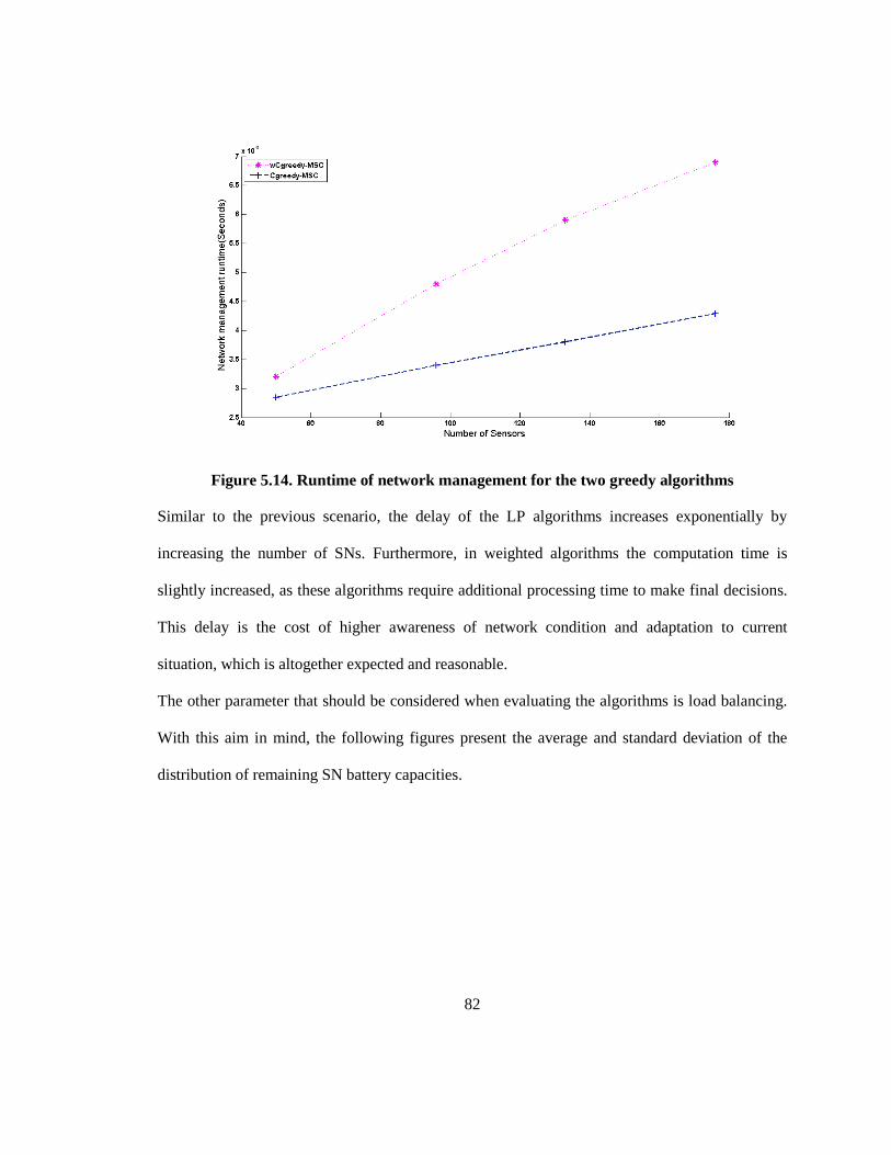
82
Figure 5.14. Runtime of network management for the two greedy algorithms
Similar to the previous scenario, the delay of the LP algorithms increases exponentially by
increasing the number of SNs. Furthermore, in weighted algorithms the computation time is
slightly increased, as these algorithms require additional processing time to make final decisions.
This delay is the cost of higher awareness of network condition and adaptation to current
situation, which is altogether expected and reasonable.
The other parameter that should be considered when evaluating the algorithms is load balancing.
With this aim in mind, the following figures present the average and standard deviation of the
distribution of remaining SN battery capacities.

83
Figure 5.15. Average of the distribution of remaining battery for all four algorithms
Figure 5.16. Average of the distribution of remaining battery for weighted algorithms

84
Figure 5.17. Average of the distribution of remaining battery for non-weighted algorithms
Figure 5.18. Standard deviation of the distribution of remained battery for all four
algorithms

85
Figure 5.19. Standard deviation of the distribution of remaining battery for weighted
algorithms
Figure 5.20. Standard deviation of the distribution of remaining battery for non-weighted
algorithms

86
Figure 5.15- Figure 5.20 likewise evidence that since the non-weighted algorithms consider
lifetime as the only criteria for network management, they show a better performance in terms of
this evaluation parameter. As it is shown, the non-weighted algorithms have less mean and
standard deviation values compared to weighted algorithms. Parallel to the first scenario, greedy
algorithms have a more balanced battery distribution.
5.3 Experimental Setup and Results
In this section, the performance of the proposed CWSN is evaluated by generating experimental
results using real wireless nodes. The purpose of this experiment is to evaluate the feasibility of
the proposed algorithms and to analyze the behavior of a real CWSN in comparison to a non-
Cognitive WSN.
Hardware and software specifications: CC2530 rev. B boards were used in this
experiment [36]. The software was developed on top of the operating system provided
by Texas Instruments for CC2530 transceivers, Z-Stack core 2.5.1. The other software
tools used are IAR Embedded Workbench v7.50A as compiler and debugger, Packet
Sniffer version 2.13.2, and User Interface V1.0 developed by us as an interface between
user and the network (the details are explained in appendix A).
Architecture: the implemented architecture is the one explained in section 3.5. There is
1 Sink Node, 1 CN, 2 R/CLH, and 6 SNs in the network. The implemented network is
shown in Figure 5.21.

87
Figure 5.21. Implementation setup
Both CWSN and non-Cognitive WSN are implemented and tested in laboratory conditions
(room’s temperature and no obstacle among nodes). The Greedy algorithm is used for creating
the set covers with a minor modification. As explained in section 5.3, there is a priority equation
to find the node’s contribution. We modified the formula in our experiments to the following one:
(5.2)
Where i is the coefficient of each parameter and can be set by CNS, Dsi is the MAC delay in the
profile table of si, LTsi is the link throughput in the profile table, and T
siN is the number of targets
that SN si covers.

88
In addition, the MAC and the routing protocols are CSMA/CA and AODV. Therefore, the
cognitive algorithm in these experiments is solely responsible for SNs’ scheduling.
In order to generate our results in a sufficiently timely manner, we set the SNs to stay in active
mode even when they are not sensing or transmitting data so they will consume more energy and
produce results faster.
Figure 5.22. Lifetime of Cognitive WSN vs. Non-Cognitive WSN
As it is shown in the Figure 5.22, the lifetime of the CWSN is longer than the non-CWSN. It is
worth to note that the CWSN is implemented with using the same nodes of a regular network and
therefore the added price of cognition is justified the outcome.
By using the designed GUI, users can have the information about current network condition as
shown in Figure 5.23.

89
Figure 5.23. Designed GUI with current information of a sample Network

90
Chapter 6
Conclusions and Future Works
6.1 Conclusions
This thesis proposes a new architecture and framework that enables cognition in WSNs. By
cognition, we mean the ability of being aware of current conditions of the network (different
nodes and surrounding environment), learning and reasoning from previous decisions, and
making appropriate decisions with the aim of satisfying user requirements.
The proposed architecture is a hierarchical one comprised of four tiers. Different types of nodes
are deployed in the network and have different responsibilities; SNs for sensing, R/CLHs for
forwarding different messages to their destinations, CNs for controlling and managing the
network, and Sink Nodes for collecting data from the network and interfacing between users and
the network.
We proposed to add a cognitive layer which controls and manages all the other layers to the
protocol stack of the network. A new node, named CN, is added to the network in order to
perform the cognitive algorithms in the network. CNs create a profile table for each node in the
network and keep themselves aware of the other nodes’ status by updating their profile tables
periodically. The cognitive management process uses the information of the profile tables in order
to take required decisions by executing decision-making process. By executing decision-making
process, CNs will schedule the nodes’ future activities (their activity mode (sleep/active),
duration of staying in this mode, and FoS).
The simulation results showed that by using cognition, the network is able to adapt itself to
changes within the network and to create a balance between different optimization goals based on

91
the current user requirements. The proposed greedy algorithm is implemented and it is shown that
the CWSN is improved the network lifetime compared to a typical WSN despite of transmitting
more control messages.
In conclusion, the proposed CWSN proved to be an intelligent network that is adaptable to the
changes and can satisfy user requirements. However, for completely enabling the cognition in
WSNs, more research should be done. In the next section, some possible future works are
discussed.
6.2 Future Works
There are several research projects that can be done to improve upon the gains we have
established in network performance. First of all, in this work we assumed that the CNs select SNs
based solely on their geographical positions. However, to have balance between CNs and
consequently a better performance, a proper algorithm should be used for assigning SNs to CNs.
We can use the procedure presented in [37] while carefully considering the issues of a CWSN. So
we can formulate the problem as following:
CNs broadcast their position (each at a different time to avoid collision). SNs wait for a certain
period of time to let all CNs send their positions. After that, SNs will send their position and a list
of CNs that they can reach. CNs then create a set of reachable SNs: a SN is in the range of a CN
if their Euclidean distance is less than the range of the CN.
(6.1)
Where RCNi is the communication range of CNi and dSj->CNi is the distance between CNi and
sensor Sj. Some sensors can communicate with more than one CN; these SNs will be categorized
as exclusive sensors.

92
(6.2)
(Please note that we assume that CNs communicate with nodes only in one-hop but sensors can
send their position via routers, in multi-hop.)
Each CN chooses SNs in ESet as its SNs. For remaining sensors, we want to assign them such
that the workload is balanced among the CNs. To achieve such a balance, we should calculate the
load on CNs; it can be formulated as:
(6.3)
Where, PLCNi is the processing load, CLCNi is the communication load, and LCNi is the load on
CNs. The processing load and communication load are formulated as:
(6.4)
Where PC is programming complexity, Ni is number of nodes per CN, fi is the frequency of
monitoring in CNi (it depends on the importance of the monitored area), and is the distance
of the farthest node assigned to the CNi. So the load is:
(6.5)
Our goal is to assign SNs such that the cognitive tasks are divided fairly among the CNs. First, we
need to find the exact function, f, and then find the optimum way of assigning nodes to CNs.
Furthermore, the employed MAC and routing protocols can be improved. For example, some
slots in the MAC should be considered for random access to the media in the case of having
mobile nodes or event-based nodes. For another research project, the FoS reference table can be
updated during network operations and MAC and Routing layers’ parameters can be used to
determine the FoS as well as the parameters of both the application and the physical layers.
93
References
[1] J. Yick, B. Mukherjee, D. Ghosal, “Wireless Sensor Networks Survey,” in Comput. Networks
52, pp. 2292-2330, 2008.
[2] I. F. Akyildiz, W. Su, Y. Sankarasubramaniam, E. Cayirci, “Wireless Sensor Networks: A
Survey,” in Elsevier Computer Network 38, pp 393-422, 2002.
[3] G. Vijay, E. Bdira, and M. Ibnkahla, “Cognitive approaches in wireless sensor networks: a
survey,” in 25th Biennial Symposium on Communications (QBSC), Kingston, 2010, pp. 177-
180.
[4] R. W. Thomas, D. H. Friend, L. A. DaSilva, and A. B. MacKenzie, “Cognitive networks:
adaptation and learning to achieve end-to-end performance objectives,” in IEEE Commun.
Mag., vol. 44, no. 12, pp. 51–57, 2006.
[5] R. W. Thomas, L. A. DaSilva, and A. B. MacKenzie, “Cognitive networks”, in First IEEE
Int. Symp. on New Frontiers in Dynamic Spectrum Access Networks, DySPAN 2005, pp. 352
– 360, 2005.
[6] D. Chen and P.K. Varshney, “QoS Support in Wireless Sensor Networks: A Survey,” Proc.
Int’l Conf. Wireless Networks (ICWN 04), CSREA Press, 2004, pp. 227-233.
[7] M. Cardee, M. T. Thai, Y. Li, W. Wu, “Energy-efficient target coverage for wireless sensor
networks,” in IEEE-INFOCOM, 1976-1984, 2005.
[8] G. Xing, X. Wang, Y. Zhang, C. Lu, R. Pless, and Christopher Gill, “Integrated coverage and
connectivity configuration for energy conservation in sensor networks,” ACM Transaction on
Sensor Network, August 2005, vol. 1, pp 36-72.
[9] A. Chamam, S. Pierre, “ on the planning of wireless sensor networks: Energy Efficient
clustering under the joint routing and coverage constraint,” in IEEE Transactions on Mobile
Computing, pp. 1077-1086, August 2009.
[10] J. N. Al-Karaki, A.E. Kamal, “Routing techniques in Wireless Sensor Networks: a survey,”
IEEE Wireless Communication, 2004, pp. 6-28.
[11] R. Verdone, D. Dardari, G. Mazzini, and A. Conti, “Wireless Sensor and Actuator Networks;
Technologies, Analysis and Design,” in Elsevier, 2008.
[12] I. Demirkol, C. Ersoy, and F. Alagoz, “MAC Protocols for Wireless Sensor Networks: a
Survey,” IEEE Communications Magazin, 2005.
[13] V. Rajendran, K. Obraczka, and J. J. Garcia-Luna-Aceves, “Energy-Efficient, Collision-Free
Medium Access Control for Wireless Sensor Networks,” in Proc. ACM SenSys, 2003.
[14] H. Nama, M. Chiang, and N. Mandayam, “Utility-Lifetime trade-off in self-regulating
Wireless Sensor Networks: A cross-layer design approach,” in Proc. IEEE ICC, 2006.
[15] S. Cui et al., “Joint Routing, MAC, and Link Layer Optimization in Sensor Networks with
Energy Constraints,” IEEE ICC 05, Korea, May 2005.

94
[16] O. B. Akan, O. Karli, and O. Ergul, “Cognitive radio sensor networks,” IEEE Network, vol.
23, no. 4, pp. 34–40, Jul.-Aug. 2009.
[17] D. Cavalcanti, S. Das, J. Wang, K. Challapali, “Cognitive Radio based wireless sensor
networks”, Proc. Seventeenth Int. Conf. Comput. Commun..and Networks, 2008. ICCCN '08,
pp. 1 - 6.
[18] L. Reznik and G. Von Pless, “Neural networks for cognitive sensor networks,” in IEEE Int.
Joint Conf. on Neural Network, IJCNN 2008, pp. 1235 – 1241, 2008.
[19] A. H. El Mougy, Z. H. Eljabi, M. Ibnkahla, and E. Bdira, “Cognitive Approaches to Routing
in Wireless Sensor Networks,” in IEEE Global Telecommunications Conference
(GLOBECOM), Miami, pp. 1-5, December 2010.
[20] H. G. Goh, K. H. Kwong, C. Shen, C. Michie, and I. Andonovic, “CogSeNet: a concept of
cognitive wireless sensor network,” in consumer communication and network conference
(CCNC) , 2010 7th IEEE, Las Vegas, NV, p. 1-2, Jan. 2010.
[21] E. Bidra and M. Ibnkahla, “Performance modeling of cognitive wireless sensor networks
applied to environmental protection,” presented at Globecom, Honolulu, Hawaii, 2009.
[22] D. Georgoulas and K. Blow, “Intelligent mobile agent middleware for wireless sensor
networks: A real time application case study,” in Proc. of the 2008 Fourth Advanced Int.
Conf. on Telecommun., AICT ‘08, pp. 95-100, 2008.
[23] S.M.A Oteafy, H. M. AboElFotoh, and H. S. Hassanein, “Dynamic Election-Based Sensing
and Routing in Wireless Sensor Networks,”in IEEE Global Telecommunications Conference,
GLOBECOM 2009, Honolulu, HI, 2009, pp. 1- 6.
[24] J. Ding et al., “A Multi-Layered Architecture and Protocols for Large-Scale Wireless Sensor
Networks,” in IEEE VTC 2003, vol. 3, pp. 1443–47, Oct. 2003.
[25] F. Aalamifar, “Iplementation of a cognitive wireless sensor network: application to
environment monitoring”, Master Thesis, Queen’s University, August 2011.
[26] F. Aalamifar, G. Vijay, P. A. Khoozani, and M. Ibnkahla, “Cognitive Wireless Sensor
Networks for Highway Safety”, Proceedings of the first ACM international symposium on
Design and analysis of intelligent vehicular networks and applications (DIVANet'11), Sept.
2011.
[27] F. Aalamifar, P. Abedi Khoozani, and M. Ibnkahla, “Multiple Cognitive Nodes in Wireless
Sensor Networks, in 26th Biennial Symposium on Communications (QBSC), Kingston, 2012.
[28] R. Harper, Inside the Smart Home, 2003: Springer-verlag
[29] T.T. Hsieh, “Using Sensor Networks for Highway and Traffic Applications,” in IEEE
Potentials, Vol. 23, No. 2, pp. 13-16, 2004.
[30] IEEE, “IEEE Standard for Information technology—Telecommunications and information
exchange between systems—Local and metropolitan area networks Specific requirements—
Part 15.4: Wireless Medium Access Control (MAC) and Physical Layer (PHY) Specifications

95
for Low-Rate Wireless Personal Area Networks (LR-WPANs),” IEEE, New York, May
2003.
[31] ZigBee, “ZigBee Profile: Telecom Applications, 1.0,” ZigBee Alliance, April 2010.
[32] P. Baronti, P. Pillai, V. W. Chook, S. Chessa, A. Gootta, Y.F., Fu, “Wireless Sensor
Networks: a survey on the state of the art and the 802.15.4 and ZigBee standards,” Computer
communication, vol. 30, 2007, pp. 1655-1695.
[33] Measuring the Power Consumption on CC2530ZNP Using CC2530 ZNP Mini Kit:
http://www.ti.com/lit/an/swra381/swra381.pdf.
[34] T. Rappaport, Wireless Communications: Principles and Practice, Prentice-Hall, Englewood
Cliffs, NJ, 1996.
[35] A. Aguiar, P. R. Pinherio, A. L. Coelho, N. Nepomuceno, A. Neto, and R. P. P. Cunha, “
Scalability analysis of a novel integer programming model to deal with energy comsumption
in heterogeneous wireless sensor netoworks,” in Lecture Notes in Computer Science, vol. 14,
pp. 11-20, 2008.
[36] CC2530 Datasheet, Available at: http://www.ti.com/litv/pdf/swrs081b.
[37] G. Gupta, M. Younis, “Load-balanced clustering in wireless sensor networks”, in Processings
of the International Conference on Communication (ICC 2003), Anchorage, Alaska, May
2003.
[38] F. Al-Turjman, H. Hassanein, and M. Ibnkahla, “Efficient deployment of wireless sensor
networks targeting environment monitoring applications”, Elsevier Computer
Communications Journal, Vol. 36, No. 2, pp. 135, Jan. 2013.
[39] F. Al-Turjman, “Grid-Based Deployment for Wireless Sensor Netowrks in Outdoor
Environment Monitoring Applications”, Ph. D. Thesis, Queen’s University, April 2011.
[40] G. Xing, X. Wang, Y. Zhang, C. Lu, R. Pless, and C. Gill, “Integrated coverage and con-
nectivity configuration for energy conservation in sensor networks”, ACM Transactions on
Sensor Networks, (1)1: 36-72, August 2005.
[41] H. Zang and J. Hou, “Maintaining sensing coverage and connectivity in large sensor
networks”, Ad Hoc and Sensor Wireless Networks: An International Journal, 1(1-2): 89-123,
Jan. 2005.
[42] S. Shakkottai, R. Srikant, and N. Shro®. Unreliable sensor grids: Coverage, connectivity, and
diameter. Ad Hoc Networks, 3(6):702-716, November 2005.
[43] S. Kumar, T. H. Lai, and J. Balogh, “on k-coverage in a mostly sleeping sensor network”, in
Proc. Of ACM MoviCom04, pp. 144-158, Philadelphia, PA, Sept. 2004.
[44] M. Ibnkahla, Ed., Adaptation and Cross Layer Design in Wireless Networks, Boca Raton:
CRC Press, 2008.
[45] G. Tolle, J. Polastre, R. Szewczyk, and D. Culler, "A macroscope in the redwoods", In Proc.
of the ACM Conf. on Embedded Networked Sensor Systems (SenSys), San Diego, 2005, pp.
51-63.

96
[46] M. Hamilton, E. Graham, P. Rundel, M. Allen, W. Kaiser, M. Hansen, and D. Estrin, "New
approaches in embedded networked sensing for terrestrial ecological observatories,"
Environmental Engineering Science, vol. 24, no. 2, pp. 192-204, Mar. 2007.
[47] R. Pon, A. Kansal, D. Liu, M. Rahimi, L. Shirachi, W. Kaiser, G. Pottie, M. Srivastava, G.
Sukhatme, D. Estrin, “Networked infomechanical systems (NIMS): next generation sensor
networks for environmental monitoring,” IEEE MTT-S International Microwave Symposium
Digest, vol. 1, pp. 373-376, June 2005.
[48] N. H., Mak and W. K. G. Seah, “How long is the lifetime of a wireless sensor network?,”
Proceedings of the IEEE 23rd
international conference on advanced information networking
and applications, AINA 2009, Bradford, UK, May 2009, pp. 763–770.
[49] F. Al-Turjman, H. Hassanein, and M. Ibnkahla, “Connectivity optimization with realistic
lifetime constraints for node placement in environmental monitoring,” In Proc. of the IEEE
Local Computer Networks (LCN), Zürich, 2009, pp. 617-624.
[50] L. van Hoesel, T. Nieberg, J. Wu, and P. Havinga, “Prolonging the lifetime of wireless sensor
networks by cross layer interaction,” IEEE Wireless Communications, vol. 11, no. 6, pp. 78-
86, Dec. 2004.
[51] X. Bai, S. Kumar, D. Xuan, Z. Yun, and T.H. Lai, “Deployeing Wireless Sensors to Achieve
Both Coverage and Connectivity,” Proc. ACM Int’l Symp, Mobile Ad Hoc Networking and
Computing, pp. 131-142, 2006.
[52] Y. Ye, “An O(n3l) potential reduction algorithm for linear programming,” Mathematical
programming, Vol 50, pp. 239-258, 1991.

97
Appendix A
Pseudo Code and Flowchart of LP solution
The pseudo-code and flow chart of the implemented LP algorithm in MATLAB is presented in
this appendix:
Pseudo-Code of LP algorithm:
#Start Process
Initialization
Set the P
For step = P to 1 do
Set ki = available battery/step ifor all s SN
While ki==0 do
#Solve the formulated LP
Set the optimal solution ( , ) 1,..., 1,...,ij jy t for i n and j p
#Remove redundancy and choose the best node
For all j = 1 to p do
Set *max
kjk i C ijt y
for all k
Set *minj k jkt t for all k
For k = 1 to m do
Calculate priority
Sort SNs based on their priority in descending order
Select the first SN with *
ij jy t
Set ij jy t
End For
End For
#Update Cover Set
Put the p created cover set in Cover Set list
#Update Remained Battery
Calculate Consumed Energy
Set 1i ik k Consumed Energy
End While
End For

98
Figure 6.1. Flowchart of implemented LP algorithm

99
Appendix B
Pseudo-code and flow chart of Greedy Solution
This Appendix provides the Pseudo-code and flow chart of implemented algorithm in MATLAB:
Pseudo-Code of Greedy algorithm:
#Start Process
Initialization
Set the P
Set Tar = list of all targets
For step = P to 1 do
Set ki = available battery/step ifor all s SN
While ki==0 do
#Start a new Cover Set
#Set the Criticality level of Targets
Calculate the minimum required Flow for each R/CLHs
Check if the available Flow in a R/CLH is less than the required, mark them as
RN with not-enough Bandwidth
Sort R/CLH with not-enough Bandwidth based on the required Bandwidth in
descending order
Set nr/clh = number of R/CLH with not-enough Bandwidth
For count = 1 to nr/clh do
Select the first R/CLH in the list
Remove all connected SNs to the selected R/CLH
Check if a Target is uncovered
Calculate SNs’ Contribution
Sort SNs based on their contribution in descending order
Select the first SN in the list
Put the SN in the current Cover set list
Remove the target from Tar
Check if the selected SN covers other targets
Removed covered targets from Tar
Remove R/CLH from R/CLH with not-enough Bandwidth
End For
For all targets remained in Tar
Sort targets based on their importance level
For targets with the same importance level
Find the median of the remained energy of related SNs
Set Criticality equal to sum of the remained energy of SNs with remained
energy higher than median
Sort targets based on their Criticality in descending order
End For
While Tar ≠ 0
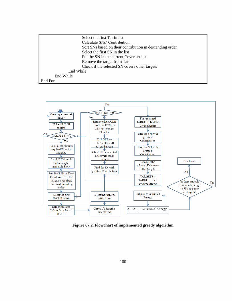
100
Select the first Tar in list
Calculate SNs’ Contribution
Sort SNs based on their contribution in descending order
Select the first SN in the list
Put the SN in the current Cover set list
Remove the target from Tar
Check if the selected SN covers other targets
End While
End While
End For
Figure 67.2. Flowchart of implemented greedy algorithm