a lagrangian random-walk model for simulating water vapor, … 1992 blm.pdf · the mode1 simulates...
TRANSCRIPT

A LAGRANGIAN RANDOM-WALK MODEL FOR SIMULATING
WATER VAPOR, CO;? AND SENSIBLE HEAT FLUX DENSITIES
AND SCALAR PROFILES OVER AND WITHIN A
SOYBEAN CANOPY
DENNIS BALDOCCHI
Atmospheric Turbulence and Diffusion Division, NOAA, P.O. Box 2456, Oak Ridge, TN 37831, U.S.A.
(Received in final form 19 March, 1992)
Abstract. An integrated canopy micrometeorological mode1 is described for calculating CO*, water vapor and sensible heat exchange rates and scalar concentration profiles over and within a crop canopy. The integrated mode1 employs a Lagrangian random walk algorithm to calculate turbulent diffusion. The integrated mode1 extends previous Lagrangian modelling efforts by employing biochemical, physio- logical and micrometeorological principles to evaluate vegetative sources and sinks. Mode1 simulations of water vapor, COP and sensible heat flux densities are tested against measurements made over a soybean canopy, while calculations of scalar profiles are tested against measurements made above and within the canopy. The mode1 simulates energy and mass fluxes and scalar profiles above the canopy successfully. On the other hand, mode1 calculations of scalar profiles inside the canopy do not match measurements.
The tested Lagrangian model is also used to evaluate simpler modelling schemes, as needed for regional and global applications. Simple, half-order closure modelling schemes (which assume a con- stant scalar profile in the canopy) do not yield large errors in the computation of latent heat (LE) and CO2 (F,) flux densities. Small errors occur because the source-sink formulation of LE and F, are relatively insensitive to changes in scalar concentrations and the scalar gradients are small. On the other hand, complicated modelling frames may be needed to calculate sensible heat flux densities; the source-sink formulation of sensible heat is closely coupled to the within-canopy air temperature profile.
1. Introduction
The evaluation of turbulent fluxes of mass and energy between the terrestrial biosphere and atmosphere is needed for a wide range of applications in the fields of atmospheric chemistry, biogeochemistry, climate modelling, ecology, hydrology, micro- and meso-meteorology and plant physiology. A hierarchy of Eulerian micrometeorological models exists for this purpose. But each model class possesses a distinct set of strengths and weaknesses. Single-layer Eulerian models are attract- ive because they are simple, rely on few input variables, and simulate surface fluxes well (Sinclair et al., 1976). On the other hand, single-layer models are limited when sources and sinks of scalars do not occur at a single layer, when controlling aerodynamic and energy properties exhibit strong gradients within a plant canopy, and when counter-gradient transfer occurs (Raupach and Finnigan, 1988; Shuttleworth, 1991).
Boundary-Layer Meteorology 61: 113-144, 1992. 0 1992 Kluwer Academic Publishers. Printed in the Netherlands.
114 DENNIS BALDOCCHI
A suite of multi-layer, Eulerian closure’ models has been developed to circum- vent some limitations associated with single-layer models (Waggoner et al., 1969; Sinclair et al., 1976; Goudriaan, 1977; Norman, 1979; Finnigan, 1985; Meyers and Paw U, 1987; Naot and Mahrer, 1989). The appeal of first and higher order closure models is their foundation on physical principles and an ability to simulate observed micrometeorological fluxes and profiles reasonably well (Sinclair et al., 1976; Meyers and Paw U, 1987; Naot and Mahrer, 1989). Furthermore, first-order closure models can accommodate separate sources and sinks and higher order closure models can simulate counter-gradient transfer (Raupach, 1988; Wilson, 1989). Despite their strengths, Eulerian closure models have not escaped criticism. First-order closure schemes fail when counter-gradient transport occurs (Raupach, 1988; Wilson, 1989). Higher-order closure models are flawed because gradient- transfer schemes are used to attain closure. Deardorff (1978) argues that gradient- transfer schemes are intrinsically impaired because they depend on time-indepen- dent turbulent diffusivities. Instead, turbulent diffusivities depend on time in the vicinity of sources and sinks due to near and far field diffusion.
Lagrangian models circumvent some of the problems of Eulerian models. One strength of Lagrangian models is their ability to explicitly calculate near and far field diffusion. Another strength of Lagrangian models is their capability to simul- ate counter-gradient transport (Raupach, 1988; Wilson, 1989). An extensive body of theoretical work exists on Lagrangian modelling of turbulent diffusion above and within model and real plant canopies from prescribed sources (e.g., Hunt and Weber, 1979; Durbin, 1980; Wilson et al., 1981a, 1981b, 1981c, 1983; Legg and Raupach, 1982; Legg, 1983; Thomson, 1984, 1987; Sawford, 1985; Leclerc et al., 1988; Raupach, 1987, 1988). Yet, the Lagrangian framework has not received wide attention for modelling heat, water vapor and CO2 exchange in real plant canopies.
Several challenges arise when applying the Lagrangian framework to real plant canopies. For instance, plant canopies have multiple sources and sinks of mass and energy that are not known a priori. Furthermore, the scalar concentration field in a plant canopy depends on the vegetative source-sink strength and on turbulent diffusion, while the vegetative source-sink strength depends on the scalar concentration field. Raupach (1988, 1989a) recently proposed a promising, but untested, scheme for considering the interactions between the scalar concentration and source-sink fields. He defines a Lagrangian dispersion matrix, whose sole dependence is on the turbulent properties of the flow. Once the dispersion matrix is known, the source-sink strengths and scalar concentrations can be solved simul- taneously.
r A closure problem arises when solving the conservation equation because it contains two unknowns, the scalar concentration and its turbulent flux density, a second-moment term. To solve the conservation equation, closure can be accomplished by either parameterizing the turbulent flux covariance as a gradient-driven diffusion process or by solving rate equations for second moments, such as the turbulent flux covariance, the Reynold’s stress and turbulent kinetic energy.
A LAGRANGIAN RANDOM-WALK MODEL 115
Ideally, a comprehensive Lagrangian model for calculating C02, water vapor and sensible heat exchange over and in a crop canopy should be able to evaluate vegetative source-sink strengths on the basis of controlling biochemical, physiologi- cal and micrometeorological principles. However, the controlling biological and physical processes are often intertwined. For example, photosynthesis and respir- ation control the uptake and release of COZ. Stomata1 mechanics regulate the diffusion of carbon dioxide and water vapor molecules in and out of the leaf. Available solar energy directly drives stomata1 mechanics, photosynthetic electron transport, leaf temperature, transpiration and sensible heat exchange. Tempera- ture governs respiration. And, finally, turbulence influences boundary-layer resis- tances and controls the shape of scalar concentration profiles.
The objective of this paper is to describe and test a canopy micrometeorological model for calculating water vapor, sensible heat and CO2 exchange rates and scalar concentration profiles over and within a crop canopy. Mass and energy fluxes and scalar profiles are computed by linking a Lagrangian turbulent diffusion model with a vegetative source-sink model. The former uses a random walk algorithm while the latter is based on physical and biological principles. Model calculations of water vapor, CO* and sensible heat flux densities are tested against measurements made over a soybean canopy, while calculations of scalar profiles are tested against measurements made above and within the canopy. Once tested, the Lagrangian-based canopy mass and energy exchange model is used to guide the development of simpler modelling schemes for regional and global applications.
2. Principles of Lagrangian Modelling
The principles of Lagrangian diffusion modelling are outlined in this section. For more detail, see Lamb (1980)) Legg and Raupach (1982)) Sawford (1985)) Raupach (1988, 1989a), Thomson (1987) and Wilson (1989).
For simplicity, consider a horizontally homogeneous canopy under steady con- ditions, where only vertical diffusion is of interest. The concentration field of a scalar is related to the statistics of an ensemble of dispersing marked fluid parcels. The ensemble mean concentration, C(z, t), at a given vertical location (z) and time (t), equals:
C(z, t) = II
P(z, tlzo, fO)S(ZO~ to) dzodfo ’
where S is the diffusive source/sink strength of a scalar from a unit volume of leaves. P(z, t ( ZO, to) is the probability density function that defines whether a fluid parcel released from a point in space (zo) at time to is observed at another location and time (z, t). This approach is valid as long as the diffusivity of the turbulent field far exceeds the molecular diffusivity of the scalar (Sawford, 1985; Wilson, 1989).
116 DENNIS BALDOCCHI
Inside a plant canopy, turbulence is inhomogeneous and non-Gaussian, i.e., the mean wind velocity and its statistics vary appreciably with height and the probabil- ity density functions of velocity fluctuations are skewed and kurtotic (Wilson et al., 1982; Baldocchi and Meyers, 1988; Raupach, 1988). The probability density function, P(z, t 1 z,,, to), cannot be specified analytically in non-Gaussian, inhomo- geneous turbulence. Yet, P(z, t ( zo, to) can be determined numerically by using a Markov sequence model; P(z, t 1 zo, to) can be estimated by calculating the trajecto- ries of an ensemble of fluid parcels and determining what proportion of fluid parcels (released from zo) reside at a given height as they travel for a given time span (Raupach, 1989).
The vertical trajectory of a fluid parcel depends on its vertical position and velocity. The vertical position of each fluid parcel, z, is determined by integrating vertical velocity (W) with respect to time:
I I
Z(r) = Z(t,) + W(t) dt’ . (2) CO
The vertical velocity of fluid parcels is calculated from the Langevin equation, a stochastic differential equation for the acceleration of a velocity component (Saw- ford, 1985; Raupach, 1988). The Langevin equation calculates acceleration as a function of the memory of its velocity and a random forcing:
dW -=--W+Pdfi(t), dt
where (Y and /? are coefficients and da(t) is a Gaussian “white noise” process. The random forcing function da(t) has a mean of zero, a variance of one and a covariance of zero between subsequent random events (Sawford, 1985; Raupach, 1988).
When the vertical velocity variance increases with height, a downward drift of fluid parcels occurs in random walk models based on Equation (1) (Legg and Raupach, 1982; Wilson et al., 1981a; Leclerc et al., 1988). An artificial accumu- lation of matter occurs in heterogeneous turbulence because fluid parcels entering into a lower region with a decreased vertical velocity scale have a reduced probabil- ity of leaving that region (Raupach, 1988; Sawford, 1985). This drift is undesirable because it violates the thermodynamic constraint that an initially uniform distribu- tion of material must be maintained (Sawford, 1985; Thomson, 1987).
Several attempts have been made to develop random-walk models that remove this unrealistic accumulation of matter near the surface. One approach introduces an additional force term into the Langevin equation, which becomes a mean upward drift velocity in the Markov sequence (Wilson et al., 1981b; Legg and Raupach, 1982). A second approach is based on an expression for the higher moments of the random term in the Markov sequence (Thomson, 1984). This second approach allows non-Gaussian random forcing. However, Thomson’s 1984
A LAGRANGIAN RANDOM-WALK MODEL 117
approach has received criticism by Thomson (1987), among others, because non- Gaussian forcing yields unrealizable solutions. Consequently, Thomson (1987) proposes a new model:
dw = a(w, z, t) dt + b(w, z, t) dt, (4)
where the random increment, dt, is Gaussian with a mean of zero and variance of dt. The variables a and b are non-linear and can be defined to account for inhomogeneous turbulence. A fourth method reflects fluid parcels according to a probability calculated from the ratio of the vertical velocity variance of fluid parcel heights at successive time steps (uJz, ti+r)lUw(z, ti) (Leclerc et al., 1988). Reflection occurs if the velocity variance ratio is less than a random draw, whose value has a mean of zero and variance of one. Tests performed in the preparation of this paper show that the probability reflection method does not prevent an artificial accumulation of material near the soil surface. Low turbulence levels, near the soil, cause travel distances of fluid parcels to be small. Consequently, the ratio between a,(~, ti+l)luw(z, ti) is often near one. Since random draws greater than this ratio are rare, parcel reflections seldom occur.
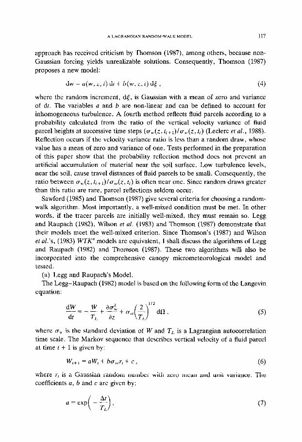
Sawford (1985) and Thomson (1987) give several criteria for choosing a random- walk algorithm. Most importantly, a well-mixed condition must be met. In other words, if the tracer parcels are initially well-mixed, they must remain so. Legg and Raupach (1982), Wilson et al. (1983) and Thomson (1987) demonstrate that their models meet the well-mixed criterion. Since Thomson’s (1987) and Wilson et al.‘s, (1983) WTK” models are equivalent, I shall discuss the algorithms of Legg and Raupach (1982) and Thomson (1987). These two algorithms will also be incorporated into the comprehensive canopy micrometeorological model and tested.
(a) Legg and Raupach’s Model. The Legg-Raupach (1982) model is based on the following form of the Langevin
equation:
!!!?=--+++a w aa2 dt TL dz ’ (5)
where (T,,, is the standard deviation of W and TL is a Lagrangian autocorrelation time scale. The Markov sequence that describes vertical velocity of a fluid parcel at time t + 1 is given by:
W t+1 =aW,+ba,r,+c, (6)
where rr is a Gaussian random number with zero mean and unit variance. The coefficients a, b and c are given by:
118 DENNIS BALDOCCHI
b=m, 09
Sawford (1985) states that the duration between successive time steps (At) of a Markov sequence must exceed the Kolmogorov acceleration time scale and be much less than the Lagrangian integral time scale. (b) Thomson’s 1987 Model.
The Thomson model defines the differential equation for fluid parcel motion as:
dW X=-T,
“+;!$($+I)+rr,(;)ii*d$, (10)
where dH is a random increment with a mean of zero and a variance equal to dt. The Markov sequence form of this equation for Gaussian turbulence and with a random increment with zero mean and unit variance (Luhar and Britter, 1989) is:
W ‘+I=W~-[~+;~(~+l)]At+uw($At~zdR. (11)
3. Model Calculations
This section describes how the random walk model was applied to calculate mass and energy exchange rates and scalar profiles over a soybean canopy. Application of the model is intended for a horizontally-homogeneous canopy that is exposed to steady ambient conditions.
3.1. THE DISPERSION MATRIX
Raupach (1988, 1989a) proposed a scheme that uses a dispersion matrix (Di,j) to compute the interdependence between S(Z, t) and C(Z). Concentration differences between an arbitrary level (Ci) and a reference level (Cr) (located above a plant canopy) are computed by summing the contributions of material diffusing to or from layers in the canopy (denoted by the subscript i):
Ci - Cr = $ Sj(Cj)Di,jAZj 3 (12) j=l
where Di,j has units of s m-l. The dispersion matrix is calculated from Equation (12) by following the trajectory of an ensemble of fluid parcels, whose source strength is prescribed and is uniform with height. Separate dispersion matrices were computed with the random-walk algorithms of Legg and Raupach (1982) and Thomson (1987).
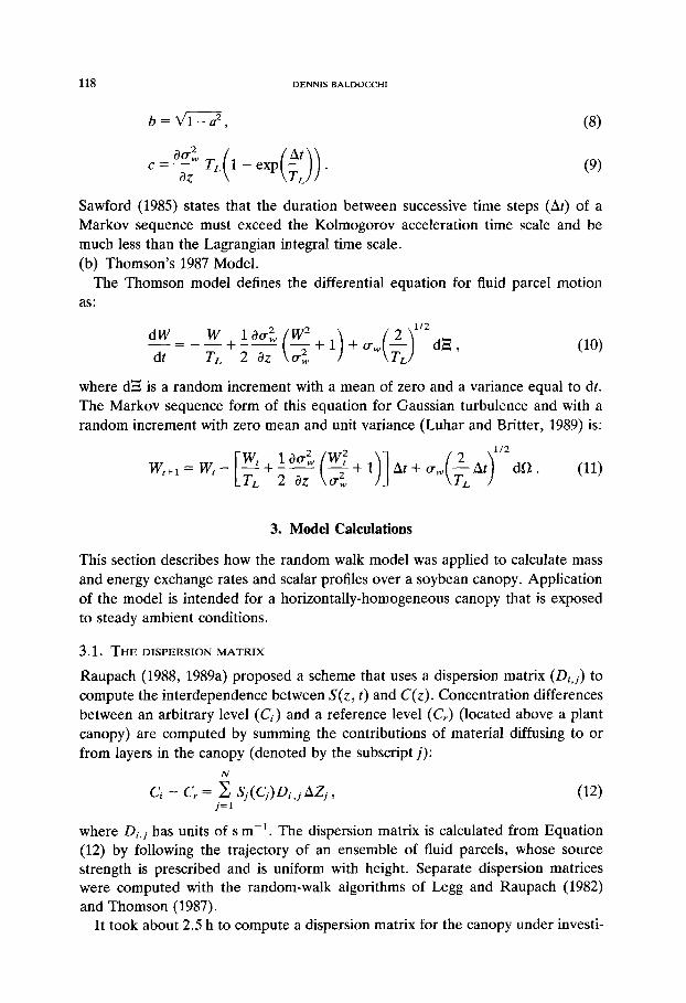
It took about 2.5 h to compute a dispersion matrix for the canopy under investi-
A LAGRANGIAN RANDOM-WALK MODEL
r2=0.95 .
slope= 1.90 .
% .’
. .
/ - 8 l
s “27 l *
_,?t
0 0 5 10 15 20 25 30
D(i,~.u*=0.55 m s-l). s m -1
119
Fig. 1. Comparison between dispersion matrices D(i,j), which were computed at friction velocities of 0.26 and 0.55 m s-l. These computations are valid for a travel time of 100 s. The r’ is 0.95 and the
slope of the regression between the two data sets is 1.90.
gation on a 386-based personal computer. To minimize excessive computational overhead, energy balance and canopy photosynthesis model runs were performed using dispersion matrices which were scaled to measured friction velocities. This scaling was justified based on data reported in Figure 1. The data show that the mean ratio between the dispersion matrices at two different friction velocities increases by 1.90 as u* increases by 2.11. The difference between these two ratios is only 11%) a tolerable error in scaled D(i) j) values.
3.2. RANDOM-WALKMODELPARAMETERS ANDTURBULENCE STATISTICS
To compute fluid parcel trajectories, we must specify the canopy’s attributes, the model domain size, the number of released fluid parcels, their travel duration, and the duration between time steps. Optimal values for these parameters were determined from sensitivity tests performed by van den Hurk and Baldocchi (1990). For computations of the dispersion matrix, the canopy was divided into 20 layers. Subsequently, 5000 fluid parcels were distributed equally among each canopy layer and released. The vertical domain over which parcels traveled con- tained 80 equally spaced layers and extended up to 4 times canopy height. It was assumed that parcels leaving the top of the domain never re-entered. Fluid parcels intercepting the soil surface were perfectly reflected upward. Fluid parcel trajecto- ries were followed for travel times up to 100 s. Longer trajectories were unnecess- ary because equilibrium concentration profiles were attained by this time (van
120 DENNIS BALDOCCHI
den Hurk and Baldocchi, 1990). Markov sequence calculations used time-steps equalling 5% of the integral time scale (7’,) at canopy height. Random numbers were computed with the rejection technique (Spanier and Gelbard, 1969).
The calculation of parcel trajectories also depends on how turbulence statistics are parameterized. Values of TL were computed with the formulation of Raupach (1988). TL was regarded as constant in the canopy and equal to 0.3hlu”. Above this height, TL was computed as TL(z) = TL(h)(zlh)0,5. The standard deviation of the vertical velocity (o,+) was parameterized to increase linearly with canopy height. Its value ranged between O.l87u* at z equal zero and 1.25u* at canopy height (h) (Raupach, 1988). Above the canopy, u, was assumed to be constant with height. These turbulence parameter values are representative of near-neutral atmospheric stability conditions and agree very well with observations within and above a crop canopy (Raupach, 1988).
3.3. SOURCE-SINK AND SCALAR CONCENTRATION FIELDS
The diffusive source/sink strength was parameterized with a resistance-analog relation (Finnigan, 1985; Meyers and Paw I-J, 1987):
w = -Paul(z) (C(z) - C(i)> Tb(Z) + r&z) (13)
where pa in air density, al(z) is leaf area density, C(z) is the scalar mixing ratio in the interstitial canopy air space, C(i) is the scalar mixing ratio inside leaves, rb is the laminar boundary-layer resistance and r, is the stomata1 resistance.
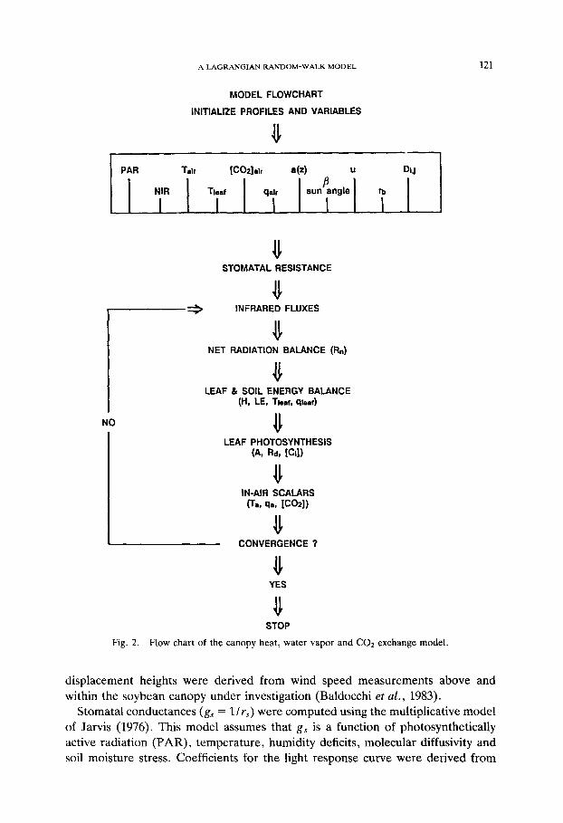
After the dispersion matrix was evaluated, concentration and vegetation source- sink fields were solved by iterating among Equations (12) and (13). The iteration scheme also accounted for interactions among governing physiological processes and abiotic factors. For example, the net radiation balance and leaf transpiration depend on leaf temperature and humidity, and vice versa. A flow chart describing the linkage between submodels is shown in Figure 2; model parameter values are listed in Table I. The modelling scheme updated infrared and net radiation flux densities, leaf and soil energy balances, leaf photosynthesis and respiration with new driving environmental conditions until desired convergence occurred.
The leaf boundary-layer resistance (Yb) was computed from theory developed for diffusion over flat plates (Grace, 1980):
1 1 0.5
- = constant - lb = d,SH 0 ,
u (14)
where d, is the molecular diffusivity, SH is the Sherwood number, 1 is the leaf length scale, and u(z) is horizontal wind speed. An exponential wind profile was assumed to calculate u(z) inside the canopy (Cionco, 1972). A logarithmic wind profile relationship was used to extend above-canopy wind speed measurements to the top of the canopy. Extinction coefficients, roughness lengths and zero-plane
A LAGRANGIAN RANDOM-WALK MODEL 121
MODEL FLOWCHART
INITIALIZE PROFILES AND VARIABLES
u
PAR Talt [Co2]alr 0)
B u
DIJ
NIR TlSd qalr sun angle m
I I I I I
u STOMATAL RESISTANCE
u
I-- 3 INFRARED FLUXES
u NET RADIATION BALANCE (Rn)
LEAF & SOIL ENERGY BALANCE (I-4 LE, Tw, wad
NO
I
LEAF PHOTOSYNTHESIS (4 Rdr [cl])
I-- IN-AIR SCALARS cr., qa# W21)
U CONVERGENCE ?
U YES
U STOP
Fig. 2. Flow chart of the canopy heat, water vapor and COz exchange model.
displacement heights were derived from wind speed measurements above and within the soybean canopy under investigation (Baldocchi et al., 1983).
Stomata1 conductances (gs = 1/ rs) were computed using the multiplicative model of Jarvis (1976). This model assumes that g, is a function of photosynthetically active radiation (PAR), temperature, humidity deficits, molecular diffusivity and soil moisture stress. Coefficients for the light response curve were derived from

122 DENNIS BALDOCCHI
TABLE I List of parameter values used to compute leaf photosynthesis, stomata1 conductance, radiative transfer,
soil evaporation and COa efflux.
Variable Unit Value Reference
Photosynthesis: Carboxylation velocity Dark respiration Quantum yield Max. photosynthesis
Stomata1 conductance Minimum resistance Light curvature coef.
Radiative transfer Leaf refl. PAR Leaf trans. PAR Soil refl. PAR Leaf refl. NIR Leaf trans. NIR Soil refl. NIR
Soil evaporation Soil resistance
Soil CO2 efflux Rsr (20 “Cl Arrhenius temperature coef.
pm01 m-* s-i pm01 m-* s-i mm01 mol-’ +mol m-* s-i
108 Harley et al. (1985) 1.91 Harley et al. (1985)
57.6 Harley et al. (1985) 81.95 Harley et al. (1985)
s m-i 50 urn01 mm2 s-l 460
s m-r
mm -2 s-1
0.083 Norman et al. (1985) 0.07 Norman et al. (1985) 0.08 Norman et al. (1985) 0.51 Walter-Shea et al. (1989) 0.47 Walter-Shea et al. (1989) 0.3 Walter-Shea et al. (1989)
2500
0.03 da Costa et al. (1986) 62468 da Costa et al. (1986)
Baldocchi, unpub. Baldocchi, unpub.
Fuchs and Tanner (1967)
field measurements made with a steady-state porometer. Stomata1 humidity re- sponses were computed using an algorithm developed by Bunce (1985) for soybeans. Stomata1 responses to temperature and humidity deficits were evaluated at the leaf surface, as advised by Collatz et al. (1991) and Grantz and Meinzer (1990). The soybean canopy was well-watered during the period under investi- gation, so no soil or leaf water potential effects were considered.
Stomata1 conductances were not updated with revised leaf temperatures and humidities. This decision was made on the basis of preliminary model tests. When stomata1 conductances were updated with new temperatures and humidity deficits, the stomata artificially slammed shut as leaf temperatures and humidity deficits exceeded certain thresholds. This numerical stomata1 closure is at odds with field measurements on soybean leaves, which instead show that g, decreases hyperboli- cally when humidity deficits are imposed by varying leaf temperature and holding ambient humidity constant (Collatz et al., 1991). One can also argue, from a modelling standpoint, that it is inappropriate to apply the Jarvis (1976) model in an iterative mode. The Jarvis model is diagnostic and does not include feedback loops among stomata1 conductance, internal CO*, transpiration, humidity deficits and leaf water potential that are described by Farquhar et al. (1978) and Jones (1983).
Radiation transfer throughout the canopy must be computed to evaluate leaf
A LAGRANGIAN RANDOM-WALK MODEL 123
photosynthesis, stomata1 conductance, and leaf energy balance. Radiative transfer routines described by Norman (1979) were used here. The probability of beam transmission through foliage spaces was computed on the assumption that the foliage was randomly distributed in space and its leaf inclination distribution was spherical. Model tests by Meyers and Paw U (1987), using data from the soybean field under investigation, show that these assumptions were valid.
The temperature and humidity at a leaf’s surface were determined from the balance between net short and longwave radiation and its partitioning into sensible (Hi) and latent heat exchange (LE1). Leaf temperature was estimated using an iterative scheme reported by Bristow (1987).
A modified form of the surface energy balance was used to evaluate the energy balance at the soil surface. In this case available energy was computed as the difference between radiation and soil heat flux densities. The resistance to vapor transfer was assumed constant since the soil surface was dry and its volumetric water content (0,) was steady; in the 0 to 0.30 m layer it ranged between 20 and 22% during the experimental period used for the model test (Baldocchi, 1982). Based on the soil moisture data and model computations reported by Fuchs and Tanner (1967) and Mahfouf and Noilhan (1991), a soil resistance of 2500 s m-l was applied.
Leaf photosynthesis (Ps) was computed using a model described by Farquhar et al. (1980) and Farquhar and von Caemmerer (1982). This method computes photosynthesis as:
P, = V, - V,l2 - Rd , (15)
where V, is the rate of carboxylation, Vo/2 is the rate of photorespiration and Rd is the rate of dark respiration. V, is the minimum between: (1) the capacity of the electron transport system to regenerate ribulose-1,5-biphosphate (RuP*); and (2) the activity of the enzyme, RuBP carboxylase-oxygenase, which initiates car- boxylation. When CO2 is scarce, the activity of RuBP carboxylase-oxygenase limits carboxylation. When CO2 is ample, photosynthesis is limited by the regeneration of RuP2, a light-dependent process. Photosynthetic calculations used photosyn- thetic parameter values that were derived from measurements on soybean leaves by Harley et al. (1985) (see Table I).
Photosynthesis, stomata1 conductance, leaf temperature and leaf transpiration are non-linear functions of light energy. Because the probability frequency distri- bution of light in the canopy is non-Gaussian, the expected value of these depen- dent functions cannot be derived on the basis of the mean light environment. Instead, these functions were evaluated according to the light incident on sunlit and shaded leaf fractions (see Norman, 1979).
Canopy CO;! flux is the difference between canopy photosynthesis (PC) and soil- root respiration (RsT). Soil-root respiration rates were calculated as a function of soil temperature, using parameterizations derived from da Costa et al. (1986); these
124 DENNIS BALDOCCHI
data were taken concurrently with the micrometeorological flux measurements described below.
The net turbulent flux of scalar material between a plant canopy and the overly- ing atmosphere was determined by integrating S(c, z) with respect to height (z) between the soil surface and the top of the canopy (15).
4. Field Measurements
Many micrometeorological and crop variables were measured to characterize the canopy, its microclimate and to compute eddy fluxes of COZ, water vapor and sensible heat. A brief overview of the experimental setup is given below. More details on the canopy and instrumentation are given by Baldocchi (1982).
Data used to test the Lagrangian model were measured over and within a Clark cultivar, soybean (Glycine mux L. Merrill). The canopy was about 1.00 m tall and had a leaf area index of 4.1 during the test periods. A continuous profile of leaf area density (al(z)) was computed by fitting a beta distribution to discrete vertical profile measurements of leaf area index (Meyers and Paw U, 1986). The crop was planted in a field that was 105 m wide and 219 m long. The main field was irrigated to maintain well-watered conditions. Surrounding fields were planted in soybeans to extend the fetch, but were not irrigated.
Net radiation flux density was measured above the canopy with a net radiometer. Net radiation profiles inside the canopy were measured with an array of strip radiometers. Soil heat flux densities were measured with soil heat flux plates, buried at 0.01 m below the surface.
The horizontal wind speed profile above the canopy was measured with sensitive cup anemometers. Wind speed profiles were measured between and within the canopy rows with omni-directional, heated thermistor anemometers. Details on above- and within-canopy wind measurements are presented in Baldocchi et al. (1983).
Temperature and water vapor pressure were measured inside and above the canopy up to a height of 3 m. A self-checking, aspirated psychrometer was used to measure temperature and humidity above the canopy (Rosenberg and Brown, 1974). Wind-aspirated, mini-psychrometers were used to measure within-canopy temperatures and humidities (Stitger and Welgraven, 1976). Shields were placed over the mini-psychrometers to protect the thermocouples from direct sunlight. The mini-psychrometers should be exposed to air speeds exceeding 4 m s-l to avoid convection errors (Fritschen and Gay, 1979). Wind speeds inside a plant canopy were much less than this value, so empirical relationships were applied to correct the mini-psychrometer output for deficient wind speed (see van den Hurk and Baldocchi, 1990).
Canopy latent and sensible heat and CO2 flux densities were inferred from micrometeorological measurements using the K-theory, flux-gradient method. Eddy exchange coefficients (K) were calculated using the energy balance method
A LAGRANGIAN RANDOM-WALK MODEL 125
(Verma and Rosenberg, 1975; Sinclair et al., 1976). Density corrections to COz flux densities were made using the theory derived by Webb et al. (1980).
Data for model testing were acquired from several days during 1979 and 1981 when the canopy was completely closed. A broad range of environmental con- ditions were used to test the model. PAR ranged between 100 and 2100 mol m-* s-l, air temperature ranged between 15” and 36°C vapor pressures ranged between 15 and 28 mb and friction velocity ranged between 0.10 and 0.65 m s-l.
5. Model Tests
5.1. FLUX DENSITIES OF ENERGY AND MASS
Calculations of energy and CO:! flux densities based on the random walk algorithms of Legg and Raupach (1982) and Thomson (1987) yielded identical results. Conse- quently, only the test of the model based on the Legg-Raupach random-walk algorithm is presented in Section 5.1.
5.1.1. Net Radiation Balance
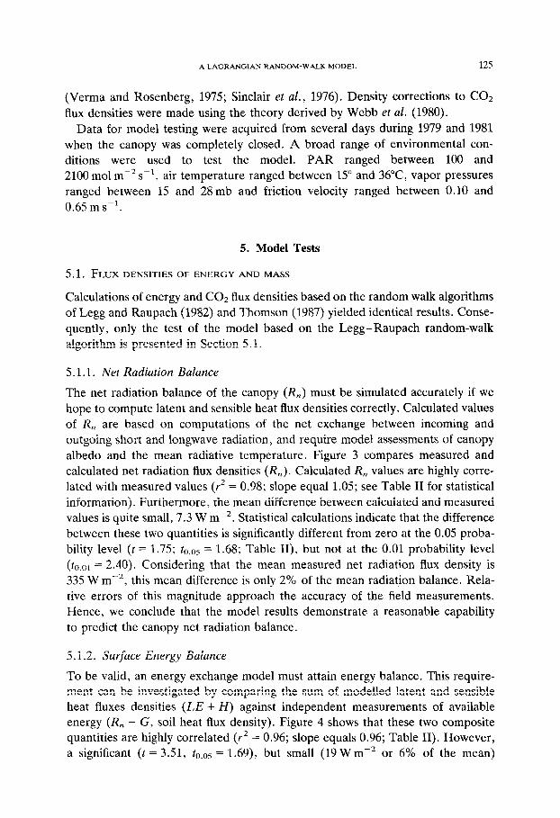
The net radiation balance of the canopy (R,) must be simulated accurately if we hope to compute latent and sensible heat flux densities correctly. Calculated values of R, are based on computations of the net exchange between incoming and outgoing short and longwave radiation, and require model assessments of canopy albedo and the mean radiative temperature. Figure 3 compares measured and calculated net radiation flux densities (R,). Calculated R, values are highly corre- lated with measured values (Y’ = 0.98; slope equal 1.05; see Table II for statistical information). Furthermore, the mean difference between calculated and measured values is quite small, 7.3 W m-‘. Statistical calculations indicate that the difference between these two quantities is significantly different from zero at the 0.05 proba- bility level (t = 1.75; t 0 05 = 1.68; Table II), but not at the 0.01 probability level (to.ol = 2.40). C onsidering that the mean measured net radiation flux density is 335 W m-*, this mean difference is only 2% of the mean radiation balance. Rela- tive errors of this magnitude approach the accuracy of the field measurements. Hence, we conclude that the model results demonstrate a reasonable capability to predict the canopy net radiation balance.
5.1.2. Surface Energy Balance
To be valid, an energy exchange model must attain energy balance. This require- ment can be investigated by comparing the sum of modelled latent and sensible heat fluxes densities (LE + H) against independent measurements of available energy (R, - G, soil heat flux density). Figure 4 shows that these two composite quantities are highly correlated (r2 = 0.96; slope equals 0.96; Table II). However, a significant (t = 3.51, t ,, 05 = 1.69), but small (19 W m-2 or 6% of the mean)

126
700
500 CG
EC 100
0
-100
DENNIS BALDOCCHI
/ 1 I , I I
r2=0.9a
Y
/
slope= 1.05 A
9
t*
J *A A A’
Y /d
A# A
-100 0 100 200 300 400 500 600 7G0 -2
Rn measured, W m
Fig. 3. Comparison between model calculations of net radiation flux density against measurements made over a soybean canopy.
500
": i 400 L
s ti 1 300 + 3:
200
100
0
1 -“.J” slope=0.96
-100 L 1 I I I , I
0 100 200 300 400 500 600
Rn - G, W m-’
Fig. 4. Comparison between model calculations of H plus LE against measurements of R, minus G values. These data apply for fluxes over the canopy.
700
600
cil 530
E s ̂ '00 -c 2 m 3 300 i: 2 u y 200
100
0
slope= 1 .OO
u 1 00 200 300 400 503 GO0 700
LE measured. W m -2
Fig. 5. Comparison between model calculations of LE against flux densities derived from applying flux-gradient theory to profile measurements. These results apply for fluxes over a soybean canopy.
A LAGRANGIAN RANDOM-WALK MODEL 127
difference exists between calculated LE plus H values and measured R, minus G values. Although perfect energy balance closure is not attained, these differences are within typical and accepted error bounds of energy balance measured over agricultural crops (?15%) (Anderson et al., 1984; Verma et al., 1989).
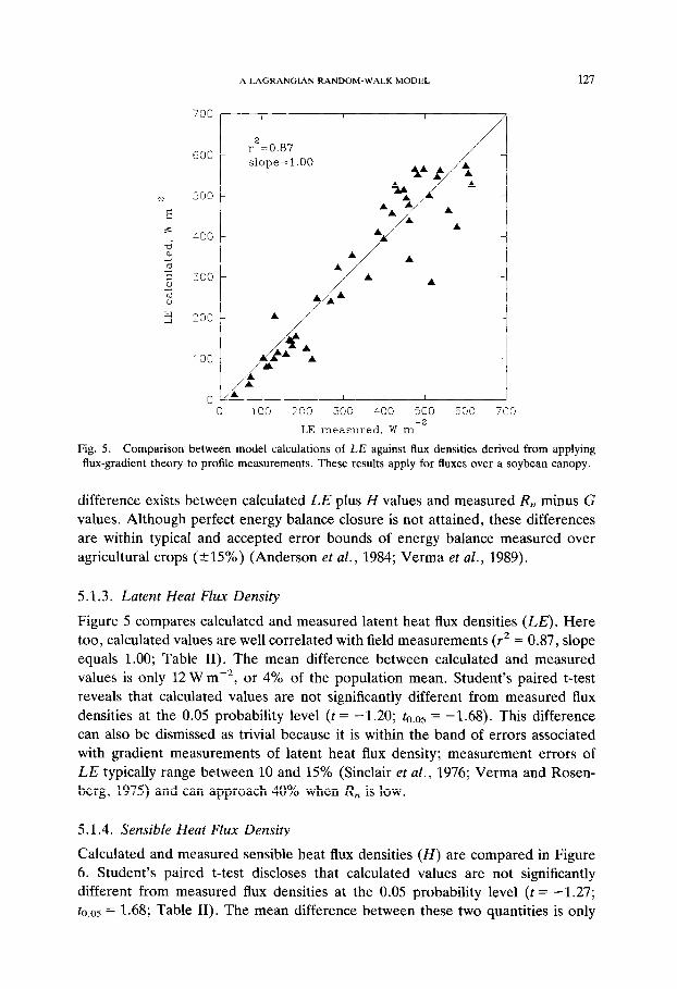
5.1.3. Latent Heat Flux Density
Figure 5 compares calculated and measured latent heat flux densities (LE). Here too, calculated values are well correlated with field measurements (r2 = 0.87, slope equals 1.00; Table II). The mean difference between calculated and measured values is only 12 W m-‘, or 4% of the population mean. Student’s paired t-test reveals that calculated values are not significantly different from measured flux densities at the 0.05 probability level (t = -1.20; to.o5 = -1.68). This difference can also be dismissed as trivial because it is within the band of errors associated with gradient measurements of latent heat flux density; measurement errors of LE typically range between 10 and 15% (Sinclair et al., 1976; Verma and Rosen- berg, 1975) and can approach 40% when R, is low.
5.1.4. Sensible Heat Flux Density
Calculated and measured sensible heat flux densities (H) are compared in Figure 6. Student’s paired t-test discloses that calculated values are not significantly different from measured flux densities at the 0.05 probability level (t = -1.27; to.o5 = 1.68; Table II). The mean difference between these two quantities is only
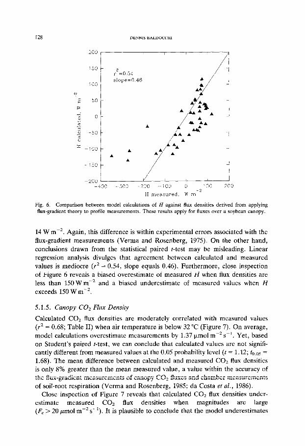
128 DENNIS BALDOCCHI
r2=0.54
slope=0.46
Fz
-100
/ ‘ A A
i
A A A
-150 1
A
-200 , .il; , / (
-400 -300 -200 -100 0 IOC 200 -2
H measured, W m
Fig. 6. Comparison between model calculations of H against flux densities derived from applying flux-gradient theory to profile measurements. These results apply for fluxes over a soybean canopy.
14 W m-*. Again, this difference is within experimental errors associated with the flux-gradient measurements (Verma and Rosenberg, 1975). On the other hand, conclusions drawn from the statistical paired t-test may be misleading. Linear regression analysis divulges that agreement between calculated and measured values is mediocre (r* = 0.54, slope equals 0.46). Furthermore, close inspection of Figure 6 reveals a biased overestimate of measured H when flux densities are less than 150 W m-* and a biased underestimate of measured values when H exceeds 150 W m-*.
5.1.5. Canopy CO2 Flux Density
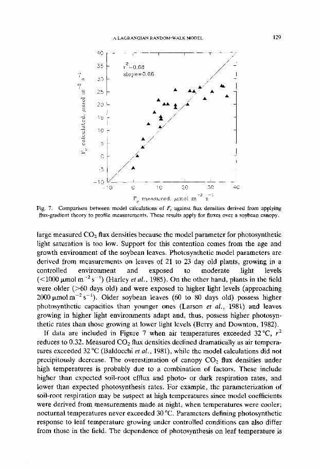
Calculated CO2 flux densities are moderately correlated with measured values (T* = 0.68; Table II) when air temperature is below 32 “C (Figure 7). On average, model calculations overestimate measurements by 1.37 umol m-2 s-r. Yet, based on Student’s paired t-test, we can conclude that calculated values are not signifi- cantly different from measured values at the 0.05 probability level (t = 1.12; to.os = 1.68). The mean difference between calculated and measured CO2 flux densities is only 8% greater than the mean measured value, a value within the accuracy of the flux-gradient measurements of canopy CO2 fluxes and chamber measurements of soil-root respiration (Verma and Rosenberg, 1985; da Costa et al., 1986).
Close inspection of Figure 7 reveals that calculated CO2 flux densities under- estimate measured CO2 flux densities when magnitudes are large (F, > 20 pm01 m -’ s-i). It is plausible to conclude that the model underestimates
A LAGRANGIAN RANDOM-WALK MODEL 129
1 (0 30 N
E 25
-10 -
i r2=0.G8 1
slope=O.GG
/ A AA i A
0 10 20 30 -2 -1
Fc measured, /Lmol m s
40
Fig. 7. Comparison between model calculations of F, against flux densities derived from applying flux-gradient theory to profile measurements. These results apply for fluxes over a soybean canopy.
large measured CO;? flux densities because the model parameter for photosynthetic light saturation is too low. Support for this contention comes from the age and growth environment of the soybean leaves. Photosynthetic model parameters are derived from measurements on leaves of 21 to 23 day old plants, growing in a controlled environment and exposed to moderate light levels (4000 km01 m -’ s-l) (Harley et al., 1985). On the other hand, plants in the field were older (~60 days old) and were exposed to higher light levels (approaching 2000 km01 m -* SK’). Older soybean leaves (60 to 80 days old) possess higher photosynthetic capacities than younger ones (Larson et al., 1981) and leaves growing in higher light environments adapt and, thus, possess higher photosyn- thetic rates than those growing at lower light levels (Berry and Downton, 1982).
If data are included in Figure 7 when air temperatures exceeded 32 “C, r2 reduces to 0.32. Measured CO2 flux densities declined dramatically as air tempera- tures exceeded 32 “C (Baldocchi et al., 1981), while the model calculations did not precipitously decrease. The overestimation of canopy CO;? flux densities under high temperatures is probably due to a combination of factors. These include higher than expected soil-root efflux and photo- or dark respiration rates, and lower than expected photosynthesis rates. For example, the parameterization of soil-root respiration may be suspect at high temperatures since model coefficients were derived from measurements made at night, when temperatures were cooler; nocturnal temperatures never exceeded 30 “C. Parameters defining photosynthetic response to leaf temperature growing under controlled conditions can also differ from those in the field. The dependence of photosynthesis on leaf temperature is
130 DENNIS BALDOCCHI
very plastic, and will shift depending on the temperature conditions under which the plants are grown (Bjorkman, 1980; Long, 1985). Obviously, an area where the canopy mass and energy exchange model can be improved is by incorporating a better understanding of the effects of environmental stress on photosynthesis and physiology. The photosynthesis and stomata1 conductance routines reported by Collatz et al. (1991) merit implementation and testing.
5.2. SCALAR PROFILES
In this section, model calculations based on the Legg-Raupach and Thomson random-walk algorithms are compared and tested against field measurements.
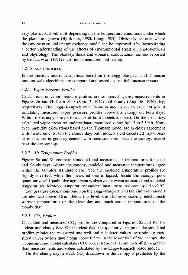
5.2.1. Vapor Pressure Profiles
Calculations of vapor pressure profiles are compared against measurements in Figures 8a and 8b for a clear (Sept. 3, 1979) and cloudy (Aug. 16, 1979) day, respectively. The Legg-Raupach and Thomson models do an excellent job of simulating measured vapor pressure profiles above the canopy on both days. Within the canopy, the performance of both models is mixed. On the clear day, calculated vapor pressures underestimate measured values by 1.5 to 2.5 mb. How- ever, humidity calculations based on the Thomson model are in closer agreement with measurements. On the cloudy day, both models yield calculated vapor pres- sures that are in good agreement with measurements inside the canopy, except near the canopy top.
5.2.2. Air Temperature Profiles
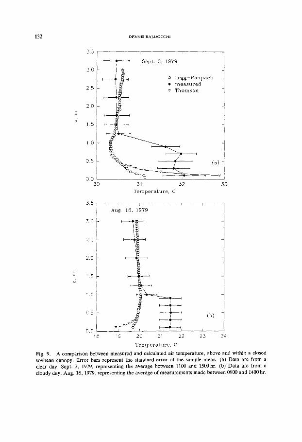
Figures 9a and 9b compare simulated and measured air temperatures for clear and cloudy days. Above the canopy, modeled and measured temperatures agree within the sample’s standard error. Yet, the modeled temperature profiles are slightly inverted, while the measured one is lapsed. Inside the canopy, poor quantitative and qualitative agreement is observed between measured and modeled temperatures. Modeled temperatures underestimate measured ones by 1.5 to 2 “C.
Temperature calculations based on the Legg-Raupach and the Thomson models are identical above 0.5 m. Below this level, the Thomson model predicts much warmer temperatures on the clear day and much cooler temperatures on the cloudy day.
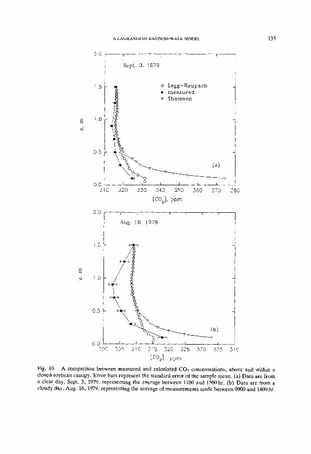
5.2.3. CO2 Profiles
Calculated and measured CO2 profiles are compared in Figures 10a and lob for a clear and cloudy day. On the clear day, the qualitative shape of the simulated profiles mimics the measured one well and calculated values overestimate mea- sured values by less than 5 ppm above 0.5 m. In the lower half of the canopy, the Thomson-based model calculates COZ concentrations that are up to 40 ppm greater than measurements and values calculated by the Legg-Raupach based model.
On the cloudy day, a weak COZ drawdown in the canopy is predicted by the
A LAGRANGlAN RANDOM-WALK MODEL 131
3.5 1
Sep 3, 1979 I 3.0
2.5
2.0
E vi 1.5
1 .o
0.5
0.0 20 21 22 23 24 25 26 27 28
vapor pressure. mb
3.5 I /
Aug. 16, 1979
vapor pressure, mb
Fig. 8. A comparison between measured and calculated vapor pressure, above and within a closed soybean canopy. Error bars represent the standard error of the sample mean. (a) Data are from a clear day, Sept. 3, 1979, representing the average between 1100 and 1500 hr. (b) Data are from a cloudy day, Aug. 16,1979, representing the average of measurements made between 0900 and 1400 hr.
132 DENNIS BALDOCCHI
3.5
3.0
2.5
2.0
E
N' 1.5
1 .o
0.5
0.0
0 Legg-Raupach l measured v Thomson
30 31 32 33
Temperature, C
35 1 I 1 I I
Aug. 16, 1979
3.0 -
2.5 -
Temperature, C
Fig. 9. A comparison between measured and calculated air temperature, above and within a closed soybean canopy. Error bars represent the standard error of the sample mean. (a) Data are from a clear day, Sept. 3, 1979, representing the average between 1100 and 1500 hr. (b) Data are from a cloudy day, Aug. 16, 1979, representing the average of measurements made between 0900 and 1400 hr.
A LAGRANGIAN RANDOM-WALK MODEL
2.0 , / I 1 I / 1
Sept. 3, 1979
o Legg-Raupach l measured v Thomson
2.0
1.5
E
l-i 10
0.5
0.0 t
[CO,l. ppm
133
310 320 330 340 350 360 370 350
300 305 310 315 320 325 330 335 CC
[C021, ppm
Fig. 10. A comparison between measured and calculated CO2 concentrations, above and within a closed soybean canopy. Error bars represent the standard error of the sample mean. (a) Data are from a clear day, Sept. 3, 1979, representing the average between 1100 and 1.500 hr. (b) Data are from a cloudy day, Aug. 16,1979, representing the average of measurements made between 0900 and 1400 hr.

134 DENNIS BALDOCCHI
TABLE II Statistics between measured and calculated flux densities
Variable Int. Slope r2 df t Mean diff.
R,, W me2 -7.8 1.05 0.98 43 1.75 7.3 H+LEvsR, 24.7 0.96 0.98 35 3.51 19 LE, W m-2 -12.3 1.00 0.87 43 -1.20 12 H, Wmm2 -12.4 0.46 0.54 43 -1.27 14 Fe, pm01 me2 s-l 6.85 0.66 0.68 23 1.12 1.37 H, with const T -48 0.261 0.261 35 2.588 40.9 LE, with const q -10.1 0.968 0.998 39 15.1 21.3
Legg-Raupach model while a moderate drawdown is measured. Both models simulated CO2 levels in the upper half of the canopy that are as much as 6 ppm greater than measured values. In the lower half of the canopy, the Thomson model calculates COz concentrations that exceed measurements by 15 ppm, while the Legg-Raupach model calculates concentrations that underestimate measured val- ues by less than 4 ppm.
5.3. DISCUSSION
5.3.1. Water Vapor, COz, and Sensible Heat Flux Densities
A validated canopy mass and energy exchange model can be used as a tool to investigate the relative control of physiological and environmental factors. One of the key physiological factors affecting mass and energy exchange is stomata1 resistance. Consequently, it is worthwhile to examine the model’s sensitivity to changes in this variable. Disregarding secondary feedbacks amongst g,, leaf temperature and humidity deficits (Figure 2) seems admissible since the model successfully predicts measured latent heat exchange over a wide range of con- ditions. On the other hand, it can be shown that the computations of latent heat and COz flux densities are quite sensitive to parameters describing the response of stomata1 resistance to light (Table III). For example, doubling the measured minimum stomata1 resistance (from 50 to 100 s m-l) reduces LE and canopy photosynthesis (PC) by about half. Correct characterization of the curvature coef- ficient associated with the response of stomata (b,) to light is also important. Halving the b, value leads to a 25% overestimate in LE, but only a 10% overesti- mate in P,. On the other hand, ignoring vapor pressure deficit effects on stomata1 resistance has moderate consequences. Model simulations conducted without this effect overestimated LE and canopy photosynthesis by about 10%.
Since LE and P, are very sensitive to stomata1 characteristics, it would be best advised to obtain stomata1 parameters for plants growing in the field under study, and not rely on data gleaned from the literature. Unfortunately, this need of pertinent model parameters is a drawback of using a comprehensive model in regional and global scale models.
A LAGRANGIAN RANDOM-WALK MODEL 135
2.5 - I / I o Legg-Raupach /
’ 1 I
l Thomson
2.0 -
0.0 , , ,
0.00 0.25 0.50 0.75 1.00 1.25 1.50 7.75 2.00
normalized concentration
Fig. 11. A test of Legg-Raupach and Thomson random walk models for meeting the well-mixed criterion. Equal number fluid parcels were released for layers throughout the model domain.
5.3.2. Scalar Projiles
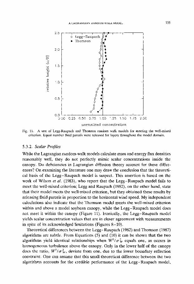
While the Lagrangian random-walk models calculate mass and energy flux densities reasonably well, they do not perfectly mimic scalar concentrations inside the canopy. Do deficiencies in Lagrangian diffusion theory account for these differ- ences? On examining the literature one may draw the conclusion that the theoreti- cal basis of the Legg-Raupach model is suspect. This assertion is based on the work of Wilson et al. (1983), who report that the Legg-Raupach model fails to meet the well-mixed criterion; Legg and Raupach (1982), on the other hand, state that their model meets the well-mixed criterion, but they obtained these results by releasing fluid parcels in proportion to the horizontal wind speed. My independent calculations also indicate that the Thomson model meets the well-mixed criterion within and above a model soybean canopy, while the Legg-Raupach model does not meet it within the canopy (Figure 11). Ironically, the Legg-Raupach model yields scalar concentration values that are in closer agreement with measurements in spite of its acknowledged limitations (Figures S-10).
Theoretical differences between the Legg-Raupach (1982) and Thomson (1987) algorithms are subtle. From Equations (5) and (10) it can be shown that the two algorithms yield identical relationships when W’/u k equals one, as occurs in homogeneous turbulence above the canopy. Only in the lower half of the canopy does the ratio, W2/a$, deviate from one, due to the lower boundary reflection constraint. One can assume that this small theoretical difference between the two algorithms accounts for the credible performance of the Legg-Raupach model,
136 DENNIS BALDOCCHI
in spite of the fact that it fails to meet the well-mixed criterion within a plant canopy.
One reason why both models may fail to perfectly simulate scalar profiles involves the role intermittency has on turbulent transfer of mass and energy and on the evolution of scalar profiles. Turbulent transfer occurs by way of quick sweeps and ejections, followed by a longer quiescent period and a ramping of the concentration of scalar material (Denmead and Bradley, 1985; Gao et al., 1989; Bergstrom and Hogstrom, 1989). The within-canopy profile of a measured scalar is, thereby, heavily weighted by the duration of the quiescent period. For example, during the quiescent period relatively great drawdowns or build-up of a scalar can occur in comparison to the well-mixed scalar profile that occurs during a sweep- ejection event (Denmead and Bradley, 1985). To illustrate this point, consider the time evolution of a normalized and vertically uniform scalar profile. For simplicity assume that the profile has a value of 0 during the well-mixed phase and a value of 1 during the relatively calm phase. If the time apportioned to the two phases is equal (as when turbulence is Gaussian), the time-averaged profile equals 0.5. In reality, the length of the ‘calm’, ramping period and the length of the well-mixed period are not equal. For instance, Collineau and Brunet (1992) show a ramping phase of temperature inside a conifer forest that occurs over a 25 s period, while a sharp drop in temperature, in association with the well-mixed sweep-ejection phase occurs over a shorter 5 s interval. If we assume, for simplicity, that the calm phase occurs 80% of the time and the mixed phase happens during 20% of the time, then the time-averaged profile equal 0.8. Consequently, the hypothetical time-averaged profile from the non-Gaussian scenario is 38% greater than the profile for the Gaussian scenario. Furthermore, the concept just illustrated is consistent with the biased difference between measured and modeled scalar profiles - the CO2 drawdown and heat and moisture build-ups measured within the canopy exceeded those simulated. Based on these arguments, it seems worth- while to incorporate the effects of skewed turbulence into the Thomson (1987) model.
Regarding air temperature profiles, it is tempting to assume that the temperature computations are valid and to suspect that the 1.5 to 2 “C jump between above- and within-canopy temperature measurements (Figure 9) was due to a bias error. Yet, an inspection of measurement errors does not support this conclusion. Abso- lute thermocouple measurements have an accuracy of kO.2 “C (Fritschen and Gay, 1979). Direct and reflected radiation errors on the thermocouples can also be discounted. All thermocouple junctions were shaded from the sun. Furthermore, energy balance computations suggest that radiation errors, under worst conditions, were less than 0.2 “C (Stitger and Welgraven, 1976). Spatial sampling bias was not a factor since spatial variability near the top of the canopy was less than 0.1 “C. Inside the canopy, spatial bias was minimized by averaging the output from three sensors that were distributed across the crop row.
Since temperature measurement errors generally can be discounted, we must
1.5
1.0 I ‘N
0.5
0
A LAGRANGlAN RANDOM-WALK MODEL
Soybeans SeDt. 3, 1979
I I I
I I
I ’
-*- Measured --- Soil Resp: 0.078 mg m-2 s1 ---- 0.05 mg m-2s1 - - 0.025 mg m-2 s-l
-
137
314 319 324 329 CO, Concentration (ppm)
334
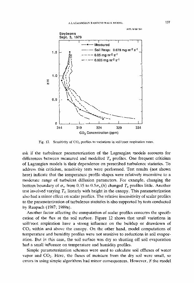
Fig. 12. Sensitivity of COz profiles to variations in soil/root respiration rates.
ask if the turbulence parameterization of the Lagrangian models accounts for differences between measured and modelled T, profiles. One frequent criticism of Lagrangian models is their dependence on prescribed turbulence statistics. To address this criticism, sensitivity tests were performed. Test results (not shown here) indicate that the temperature profile shapes were relatively insensitive to a moderate range of turbulent diffusion parameters. For example, changing the bottom boundary of (T, from 0.15 to OSa,(h) changed T, profiles little. Another test involved varying TL linearly with height in the canopy. This parameterization also had a minor effect on scalar profiles. The relative insensitivity of scalar profiles to the parameterization of turbulence statistics is also supported by tests conducted by Raupach (1987; 1989a).
Another factor affecting the computation of scalar profiles concerns the specifi- cation of the flux at the soil surface. Figure 12 shows that small variations in soil/root respiration have a strong influence on the buildup or drawdown of CO2 within and above the canopy. On the other hand, model computations of temperature and humidity profiles were not sensitive to reductions in soil evapor- ation. But in this case, the soil surface was dry so shutting off soil evaporation had a small influence on temperature and humidity profiles.
Simple parameterization schemes were used to calculate soil effluxes of water vapor and CO 2. Here, the fluxes of moisture from the dry soil were small, so errors in using simple algorithms had minor consequences. However, if the model

138 DENNIS BALDOCCHI
is to be applied under a wider range of canopy cover and soil moisture conditions, improved soil evaporation schemes will be necessary. Mahfouf and Noilhan (1991) recently reviewed a variety of soil evaporation methods that could be implemented. Soil CO2 efflux is a more elusive quantity to model mechanistically, since it depends on contributions from roots and microbes. Unfortunately, abiotic-driven algorithms, as used here, represent the state-of-the-art (see Carlyle and Than, 1988).
In the introduction, strengths and weakness of Eulerian and Lagrangian models were identified. How well do Lagrangian and Eulerian models compare in their ability to compute scalar profiles of temperature and humidity? In surveying the literature, I found that within-canopy temperature and humidity profiles computed by both Lagrangian and Eulerian models do not match field measurements (Goud- riaan, 1977: maize, K-theory model, T and q; Meyers and Paw U, 1987: soybeans, higher-order closure, T, and Naot and Mahrer, 1989: cotton, higher-order closure, 0
5.3.3. Application : Testing Model Parameterization Schemes
In regional and global-scale climate, ecology and chemistry models, it is desirable to specify lower boundary fluxes of mass and energy with a simple model instead using a cumbersome particle trajectory or higher order closure model. One use of the validated and detailed micrometeorological model is as a tool for guiding the development of simpler parameterization schemes. For example, by intercompar- ing flux measurements with a detailed canopy micrometeorological model and a simpler closure scheme, one can evaluate how the ability to estimate fluxes changes with changing model sophistication. Theoretically, source-sink strengths are de- pendent on the scalar field and vice versa. If strong gradients exist inside a plant canopy and the source-sink term is sensitive to the scalar concentration, it can be argued that a micrometeorological model, which resolves the local concentration field, is required to calculate fluxes. On the other hand, one could argue that simple half-order closure models2 would be useful if the scalar concentration profile is uniform or if the source-sink parameterization is insensitive to changes in scalar quantity.
Before testing whether we need a simple or complex parameterization scheme for calculating sensible heat exchange (H), let us first investigate how sensitive H is to observed drawdowns or build-ups in air temperature (T,). We can define this sensitivity by using elementary calculus to determine the partial derivative of H with respect to air temperature:
aH b(z) P&J -=- dTC2 r,
(16)
’ Half-order closure models integrate the source-sink term (Equation (13)) with respect to height by assuming that a scalar profile is constant.
A LAGRANGIAN RANDOM-WALK MODEL 139
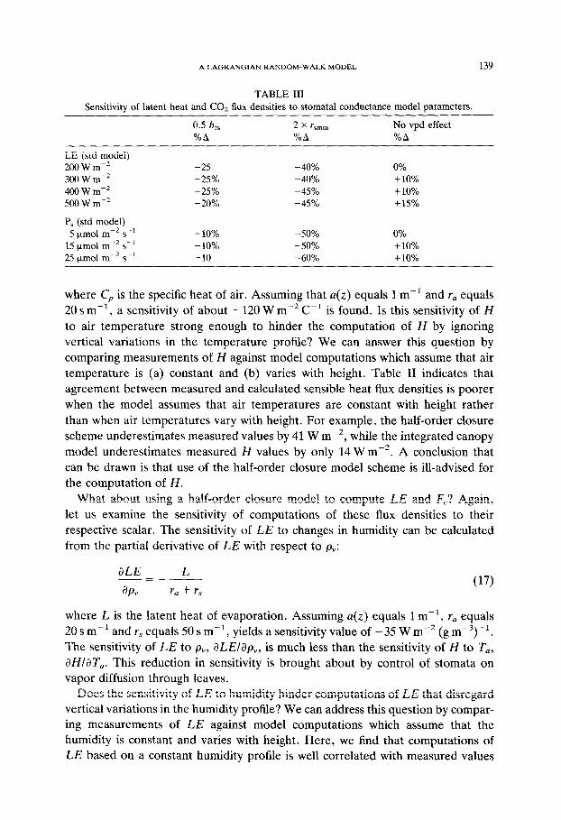
TABLE III Sensitivity of latent heat and CO2 flux densities to stomata1 conductance model parameters.
0.5 b,, %A
2 x rsmin %A
No vpd effect %A
LE (std model) 200 W m-’ 300 W me2 400 W me2 500Wm-2
P, (std model) 5 hmol m-* s-l
15 pm01 m-* s-l 25 &mol m-* s-l
+25 -40% 0% +25% -40% +lo% +25% -45% + 10% +20% -45% +15%
+ 10% -50% 0% +lo% -50% +10% +10 -60% +10%
where C, is the specific heat of air. Assuming that a(z) equals 1 m-r and r, equals 20sm-l, a sensitivity of about -120 W me2 C-l is found. Is this sensitivity of H to air temperature strong enough to hinder the computation of H by ignoring vertical variations in the temperature profile? We can answer this question by comparing measurements of H against model computations which assume that air temperature is (a) constant and (b) varies with height. Table II indicates that agreement between measured and calculated sensible heat flux densities is poorer when the model assumes that air temperatures are constant with height rather than when air temperatures vary with height. For example, the half-order closure scheme underestimates measured values by 41 W rne2, while the integrated canopy model underestimates measured H values by only 14 W m-*. A conclusion that can be drawn is that use of the half-order closure model scheme is ill-advised for the computation of H.
What about using a half-order closure model to compute LE and F,? Again, let us examine the sensitivity of computations of these flux densities to their respective scalar. The sensitivity of LE to changes in humidity can be calculated from the partial derivative of LE with respect to a:
(17)
where L is the latent heat of evaporation. Assuming a(z) equals 1 m-l, r, equals 20 s m-r and rS equals 50 s m-l , yields a sensitivity value of -35 W m-* (g mM3)-l. The sensitivity of LE to pv, dLE/ap,, is much less than the sensitivity of H to T,, aH/aT,. This reduction in sensitivity is brought about by control of stomata on vapor diffusion through leaves.
Does the sensitivity of LE to humidity hinder computations of LE that disregard vertical variations in the humidity profile? We can address this question by compar- ing measurements of LE against model computations which assume that the humidity is constant and varies with height. Here, we find that computations of LE based on a constant humidity profile is well correlated with measured values
140 DENNIS BALDOCCHI
(r2 = 0.99; slope = 0.968; Table II) differing by only 21 W rnd2. Considering that LE values during midday range between 400 and 600 W rne2, a 21 W mP2 differ- ence is trivial during this period. Furthermore, the performance of the half-order closure model is not much worse than the performance of the integrated Lagrang- ian model, which differed from measured values by 12 W rne2. Based on these calculations, it can be concluded that a simple half-order parameterization scheme can be used to calculate LE under certain conditions; the scheme will work best when r, is much greater than rb.
The influence of assuming a constant CO2 profile on the computation of canopy CO2 exchange has been addressed in another analysis (Baldocchi, 1992). It was shown for soybeans and a deciduous forest that computations of Fe are relatively insensitive to variations in the CO1 profile, so a half-order closure scheme is valid for modelling this variable too.
6. Conclusion
C02, water vapor and sensible heat exchange rates over a soybean canopy can be successfully computed with a Lagrangian random-walk model, based on the algo- rithm of either Legg and Raupach (1982) or Thomson (1987). On the other hand, model calculations of scalar profiles inside the canopy do not match measurements. The neglect of intermittency may partly explain this poor model performance. Algorithms that account for non-Gaussian turbulence need to be tested inside crop and forest canopies to resolve this issue. Lagrangian models incorporating Thomson’s (1987) algorithm for skewed turbulence have been successfully tested in the planetary boundary layer (Luhar and Britter, 1990) and can easily be adapted for use in plant canopies.
The Lagrangian model was also used to test simpler modelling schemes, as needed for regional and global applications. Using simple, half-order closure modelling schemes (they assume constant scalar profiles in the canopy) do not yield large errors in the computation of latent heat (LE) and CO* (F,) flux densities. Small errors occur because the source-sink formulation of LE and F, are relatively insensitive to changes in scalar concentrations. On the other hand, complicated modelling frames are needed to calculate sensible heat flux densities. For this latter case, the source-sink formulation of sensible heat is closely coupled to the within-canopy air temperature profile. Overall, sensitivity tests reveal that model calculations of mass and energy exchange are more sensitive to the par- ameterization of physiological variables than to turbulence quantities.
Acknowledgements
The modelling work was partially supported by the National Oceanic and Atmo- spheric Administration and the U.S. Department of Energy. Gratitude is ex- pressed to Bart van den Hurk, who assisted me in the early phase of this work.
A LAGRANGIAN RANDOM-WALK MODEL 141
Conversations with Dr. Rick Eckman and his careful and constructive review of the manuscript are much appreciated. I also thank Dr. David Hollinger, for providing me with a version of the Farquhar-von Caemmerer photosynthesis model, and Dr. Shashi Verma, who assisted and funded me during the field measurements.
References
Anderson, D. E., Verma, S. B., and Rosenberg, N. J.: 1984, ‘Eddy Correlation Measurements of CO*, Latent Heat and Sensible Heat Fluxes over a Crop Surface’, Boundary-Layer Meteorol. 29, 263-212.
Baldocchi, D. D.: 1982, ‘Mass and Energy Exchanges of Soybeans: Microclimate-Plant Architectural Interactions; Center for Agricultural Meteorology and Climatology/Institute of Agriculture and Natural Resources/University of Nebraska-Lincoln.
Baldocchi, D.D.: 1992, ‘Scaling Water Vapor and Carbon Dioxide Exchange from Leaves to Canopies: Rules and Tools’, in J. Ehleringer and C. Field (eds.), Scaling Processes between Leaf and Landscape Levels, Academic Press, New York, in press.
Baldocchi, D. D. and Meyers, T. P.: 1988, ‘Turbulence Structure in a Deciduous Forest’, Boun- dary-Layer Meteorol. 43, 345-364.
Baldocchi, D. D., Verma, S. B., and Rosenberg, N. J.: 1981, ‘Mass and Energy Exchanges of a Soybean Canopy under Various Environmental Regimes’, Agron. J. 73, 706-710.
Baldocchi, D. D., Verma, S. B., and Rosenberg, N. J.: 1983, ‘Characteristics of Air Flow Above and Within Soybean Canopies’, Boundary-Layer Meteorol. 25, 43-54.
Bergstrom, H. and Hogstrom, U.: 1989, ‘Turbulent Exchange Above a Pine Forest. II. Organized Structures’, Boundary-Layer Meteorol. 49, 231-263.
Berry, J. A. and Downton, W. J. S.: 1982, ‘Environmental Regulation of Photosynthesis’, in Photo- synthesis: Development, Carbon Metabolism and Plant Productivity, Vol II, Academic Press, New York, pp. 263-343.
Bjorkman. 0.: 1980, ‘The Response of Photosynthesis to Temperature’, in J. Race et al. (eds.), Plants and their Atmospheric Environment, Blackwell Scientific Publications, Oxford, pp. 273-301.
Bristow, K. L.: 1987, On Solving the Surface Energy Balance Equation for Surface Temperature’, Agricultural Forest Meteorol. 39, 49-54.
Bunce, J. A.: 1985, ‘Effects of Boundary Layer Conductance on the Response of Stomata to Humidity’, Plant, Cell and Environment 8, 55-57.
Carlyle, J. C. and Than, U. B.: 1988, ‘Abiotic Controls of Soil Respiration Beneath an Eighteen-Year Old Pinus Radiata Stand in South-Eastern Australia’, J. Ecol. 76, 654-662.
Cionco, R. M.: 1972, ‘A Wind-Profile Index for Canopy Flow’, Boundary-Layer Meteorol. 3, 255- 263.
Collatz, J., Ball, J. T., Rivet, C., and Berry, J. A.: 1991, ‘Regulation of Stomata1 Conductance and Transpiration: A Physiological Mode1 of Canopy Processes’, Agricultural Forest Meteorol. 54, 107- 136.
Collineau, S. and Brunet, Y.: 1992, ‘Detection of Turbulent Coherent Motions in a Forest Canopy Layer. II. Time-Scales and Conditional Averages’, Boundary-Layer Meteorol. to be submitted.
Da Costa, J. M. N., Rosenberg, N. J., and Verma, S. B.: 1986, ‘Respiratory Release of CO1 in Alfalfa and Soybean under Field Conditions’, Agricultural Forest Meteorol. 37, 143-157.
Deardorff, J. W.: 1978, ‘Closure of Second- and Third-Moment Rate Equations for Diffusion in Homogeneous Turbulence’, Phys. Fluids 21, 525-530.
Denmead, 0. T. and Bradley, E. F.: 1985, ‘Flux-Gradient Relationships in a Forest Canopy’, in B. A. Hutchison and B. B. Hicks (eds.), Forest-Atmosphere Interactions, D. Reidel, Dordrecht, pp. 421-442.
Durbin, P. A.: 1980, ‘A Random Flight Mode1 of Inhomogeneous Turbulent Dispersion’, Phys. Fluids 23, 2151-2153.
Farquhar, G. D. and Caemmerer, S. von: 1982, ‘Modeling Photosynthetic Response to Environmental

142 DENNIS BALDOCCHI
Conditions’, in 0. L. Lange et al., (eds.), Encyclopedia of Plant Physiology 12B, Springer-Verlag, Berlin, pp. 549-587.
Farquhar, G. D., Dubbe, D. R., and Raschke, K.: 1978, Gain of the Feedback Loop Involving Carbon Dioxide and Stomata’, Plant Physiol. 62, 406-412.
Farquhar, G. D., Caemmerer, S. von, and Berry, J. A.: 1980, ‘A Biochemical Model of Photosynthetic COZ Assimilation in Leaves of C3 Species’, Planta 149, 78-90.
Finnigan, J. J.: 1985, ‘Turbulent Transport in Flexible Plant Canopies’, in B. A. Hutchison and B. B. Hicks (eds.), The Forest-Atmosphere Interaction, D. Reidel Publishing Company, Dordrecht, The Netherlands.
Fritschen, L. J. and Gay, L. W.: 1979, Environmental Instrumentation, Springer-Verlag, New York. 216 pp.
Fuchs, M. and Tanner, C. B.: 1967, ‘Evaporation from a Drying Soil’, J. Appl. Meteorol. 6, 852-857. Gao, W., Shaw, R. H., and Paw U, K. T.: 1989, ‘Observation of Organized Structure in Turbulent
Flow Within and Above a Forest Canopy’, Boundary-Layer Meteorol. 47, 349-371. Goudriaan, J.: 1977, ‘Crop Micrometeorology: a Simulation Study’, Centre for Agricultural Publishing
and Documentation, Wageningen, The Netherlands. 249 pp. Grace, J.: 1980, ‘Some Effects of Wind on Plants’, in J. Race et al. (eds.), Plants and their Atmospheric
Environment, Blackwell Scientific Publications, Oxford, pp. 31-56. Grantz, D. A., and Meinzer, F. C.: 1990, ‘Stomata1 Response to Humidity in a Sugarcane Field:
Simultaneous Porometric and Micrometeorological Measurements’, Plant, Cell and Environ. 13, 27- 37.
Harley, P. C., Weber, J. A., and Gates, D. M.: 1985, ‘Interactive Effects of Light, Leaf Temperature, CO* and O2 on Photosynthesis in Soybean’, Planta 165, 249-263.
Hunt, J. C. R. and Weber, A. H.: 1979, ‘A Lagrangian Statistical Analysis of Diffusion from a Ground-Level Source in a Turbulent Boundary Layer’, Quart. J. Roy. Metorol. Sot. 105, 423-443.
Jarvis, P. G.: 1976, ‘The Interpretation of the Variations in Leaf Water Potential and Stomata1 Conductance Found in Canopies in the Field’, Phil. Trans. Royal Sot. London, B 273, 593-610.
Jones, H.: 1983, Plants and Microclimate, Cambridge Univ. Press, Cambridge, UK. 323 pp. Lamb, R.: 1980, ‘Mathematical Principles of Turbulent Diffusion Modeling’, in A. Longhetto (ed.),
Atmospheric Boundary Layer Physics, Elsevier Sci. Pub., pp. 173-210. Larson, E. M., Hesketh, J. D., Woolley, J. T., and Peters, D. B.: 1981, ‘Seasonal Variations in
Apparent Photosynthesis Among Stands of Different Soybean Cultivars’, Photosynthetic Res. 2, 3- 20.
Leclerc, M. Y., Thurtell, G. W., and Kidd, G. E.: 1988, ‘Measurements and Langevin Simulations of Mean Tracer Concentration Fields Downwind from a Circular Line Source Inside an Alfalfa Canopy’, Boundary-Layer Meteorol. 43, 287-308.
Legg, B. J.: 1983, ‘Turbulent Dispersion from an Elevated Line Source: Markov-Chain Simulations of Concentration- and Flux-Profiles’, Quart. J. Roy. Meteorol. Sot. 109, 64.5660.
Legg, B. J. and Raupach, M. R.: 1982, ‘Markov-Chain Simulation of Particle Dispersion in Inhomo- geneous Flows: the Mean Drift Velocity Induced by a Gradient in Eulerian Velocity Variance’, Boundary-Layer Meteorol. 24, 3-13.
Long, S. P.: 1985, ‘Leaf Gas Exchange’, in J. Barber and N. R. Baker (eds.), Photosynthetic Mechan- isms and the Environment, Elsevier Sci. Pub, pp. 453-499.
Luhar, A. K. and Britter, R. E.: 1989, ‘A Random Walk Model for Dispersion in Inhomogeneous Turbulence in a Convective Boundary Layer’, Atmos. Envir. 23, 1911-1924.
Mahfouf, J. F. and Noilhan, J.: 1991, ‘Comparative Study of Various Formulations of Evaporation from Bare Soil Using in situ Data’, J. Appl. Meteorol. 30, 1354-1365.
Meyers, T. P. and Paw U, K. T.: 1986, ‘Testing of a Higher-Order Closure Model for Modeling Airflow within and above Plant Canopies’, Boundary-Layer Meteorol. 37, 297-311.
Meyers, T. P. and Paw U, K. T.: 1987, ‘Modelling the Plant Canopy Micrometeorology with Higher- Order Closure Principles’, Agricultural Forest Meteorol. 41, 143-163.
Naot, 0. and Mahrer, Y.: 1989, ‘Modeling Microclimate Environments: a Verification Study’, Boun- dary-Layer Meteorol. 46, 333-354.
Norman, J. M.: 1979, ‘Modeling the Complete Crop Canopy’, in B. J. Barfield and J. F. Gerber (eds.), Modification of the Aerial Environment of Plants, American Society of Agricultural Engineers, St. Joseph, MI, pp. 249-277.
A LAGRANGIAN RANDOM-WALK MODEL 143
Norman, J. M., Welles, J. M., and Walter-Shea, E. A.: 1985, ‘Contrasts Among Bidirectional Reflect- ance of Leaves, Canopies and Soils’, IEEE Transactions on Geoscience and Remote Sensing, E-23: pp. 659-667.
Raupach, M. R.: 1987, ‘A Lagrangian Analysis of Scalar Transfer in Vegetation Canopies’, Quart. J. R. Meteorol. Sot. 113, 107-120.
Raupach, M. R.: 1988, ‘Canopy Transport Processes’, in W. L. Steffen and 0. T. Denmead (eds.), Flow and Transport in the Natural Environment, Springer-Verlag, Berlin.
Raupach, M. R.: 1989a, ‘Applying Lagrangian Fluid Mechanics to Infer Scalar Source Distributions from Concentration Profiles in Plant Canopies’, Agric. Forest Meteorol. 47, 85-108.
Raupach, M. R.: 1989b, ‘A Practical Lagrangian Method for Relating Scalar Concentrations to Source Distributions in Vegetation Canopies’, Quart. J. Roy. Meteorol. Sot. 115, 609-632.
Raupach, M. R. and Finnigan, J. J.: 1988, ‘Single-Layer Models of Evaporation from Plant Canopies are Incorrect but Useful, Whereas Multilayer Models are Correct but Useless’, Austral. J. Plant Physiol. 15, 705-716.
Rosenberg, N. J. and Brown, K. W.: 1974, ‘Self Checking Psychrometer Systems for Gradient and Profile Determinations near the Ground’, Agric. Meteorol. 13, 215-226.
Sawford, B. L.: 1985, ‘Lagrangian Statistical Simulation of Concentration Mean and Fluctuation Fields’, J. Clim Appl. Meteorol. 24, 1152-1166.
Sawford, B. L.: 1986, ‘Generalized Random Forcing in Random-Walk Turbulent Dispersion Models’, Phys. Fluids 29, 3582-3585.
Shuttleworth, W. J.: 1991, ‘Evaporation Models in Hydrology’, in T. J. Schmugge and J. C. Andre (eds.), Land Surface Evaporation: Measurement and Parameterization, Springer-Verlag, New York, pp. 93-120.
Sinclair, T. R., Murphy, C. E., and Knoerr, K. R.: 1976, ‘Development and Evaluation of Simplified Models for Simulating Canopy Photosynthesis and Transpiration’, J. Appt. Ecol. 13, 813-829.
Spanier, J. and Gelbard, E. M.: 1969, Monte Carlo Principles and Neutron Transport Problems, Addison-Wesley Pub. Co., Reading, MA, 234 pp.
Stitger, C. J. and Welgraven, A. D.: 1976, ‘An Improved Radiation Protected Differential Psychro- meter for Crop Environment’, Arch. Met. Geophys. Biokl. 24B, 177-181.
Thomson, D. J.: 1984, ‘Random Walk Modelling of Diffusion in Inhomogeneous Turbulence’, Quart. J. R. Meteorol. Sot. 110, 1107-1120.
Thomson, D. .I.: 1987, ‘Criteria for the Selection of Stochastic Models of Particle Trajectories in Turbulent Flow’, J. Fluid Mech. 180, 529-556.
Van den Hurk, B. and Baldocchi, D. D.: 1990, ‘A Random Walk Model for Simulating Water Vapor Exchange in a Soybean Canopy’, NOAA technical report. ARL-185. 46 pp.
Verma, S. B. and Rosenberg, N. J.: 1975, ‘Accuracy of Lysimetric, Energy Balance and Stability- Corrected Aerodynamic Methods of Estimating Above Canopy Flux of CO*‘, Agron. J. 67, 699- 704.
Verma, S.B., Kim, J., and Clement, R. J.: 1989, ‘Carbon Dioxide, Water Vapor and Sensible Heat Fluxes over a Tallgrass Prairie’, Boundary-Layer Meteorol. 46, 53-67.
Waggoner, P. E., Furnival, G. M., and Reifsnyder, W. E.: 1969, ‘Simulation of the Microclimate in a Forest’, Forest Science 15, 37-45.
Walter-Shea, E. A., Norman, J. M., and Blad, B. L.: 1989, ‘Leaf Bidirectional Reflectance and Transmittance in Corn and Soybean’, Remote Sensing Environment 29, 161-174.
Webb, E. K., Pearman, G. I., and Leuning, R.: 1980, ‘Correction of Flux Measurements for Density Effects Due to Heat and Water Vapor Transfer’, Quart. J. R. Meteorol. Sot. 106, 85-100.
Wilson, J. D.: 1989, ‘Turbulent Transport Within the Plant Canopy’, in T. A. Black, D. L. Spittlehouse, M. Novak and D. T. Price (eds.), Estimation of Area1 Evapotranspiration, IAHS Press, Wallingford, UK, pp. 43-80.
Wilson, J. D., Thurtell, G. W., and Kidd, G. E.: 1981a, ‘Numerical Simulation of Particle Trajectories in Inhomogeneous Turbulence, I: Systems with Constant Turbulent Velocity Scale’, Boundary-Layer Meteorology 21, 295-313.
Wilson, J. D., Thurtell, G. W., and Kidd, G. E.: 1981b, ‘Numerical Simulation of Particle Trajectories in Inhomogeneous Turbulence, II: Systems with Variable Turbulent Velocity Scale’, Boundary-Layer Meteorol. 21, 423-441.
Wilson, J. D., Thurtell, G. W., and Kidd, G. E.: 1981c, ‘Numerical Simulation of Particle Trajectories

144 DENNIS BALDOCCHI
in Inhomogeneous Turbulence, III: Comparison of Predictions with Experimental Data for the Atmospheric Surface Layer’, Boundary-Layer Meteorol. 21, 443-463.
Wilson, J. D., Ward, D. P., Thurtell, G. W., and Kidd, G. E.: 1982, ‘Statistics of Atmospheric Turbulence Within and Above a Corn Canopy’, Boundary-Layer Meteorol. 24, 495-519.
Wilson, J. D., Legg, B. J., and Thomson, D. J.: 1983, ‘Calculation of Particle Trajectories in the Presence of a Gradient in Turbulent-Velocity Variance’, Boundary-Layer Meteorol. 27, 163-169.