Fli;' HEWLETTa:~ PACKARD

A Kinematically Stable HybridPosition/Force Control Scheme

William D. Fisher, M. Shahid MujtabaMeasurement and Manufacturing Systems LaboratoryHPL-91-154October, 1991

hybrid control,kinematicstability, robotmanipulator,Jacobian matrix,projection matrix,pseudoinverse

A correction to the position formulation of the hybridposition/force control scheme is presented. In theoriginal position formulation, the derivation that usesthe inverse of the Jacobian matrix to map fromCartesian space to joint space is shown to bealgebraically incorrect. This incorrect derivation causesthe kinematic instability attributed to the hybridposition/force control scheme. The correct derivationshows that the transformation between joint space andCartesian space involves both the selection matrix andthe Jocobian matrix, making the inverse mapping morecomplex since the two matrix transformations can nolonger be treated independently. A sufficient conditionfor system stability using only the kinematicinformation is defined. With the corrected positionformulation, the hybrid position/force control schemedemonstrates kinematically stable behavior and isapplied to an example that was previously shown to beunstable. This correction generalizes the applicability ofthe hybrid position/force control scheme by providingsystem robustness for all robot manipulators.

This report is a shorter version of "Hybrid Position/Force Control: A Correct Formulation", to bepublished in the International Journal ofRobotics Research, in 1992© Copyright Hewlett-Packard Company 1991

Internal Accession Date Only

Contents

1 Introd uction and Background

2 The Position Related Equations

3 A Correction to the Position Formulation

4 A Comparison to the Original Position Solution

5 A Stable Hybrid Control Scheme

6 A Test Case: The An and Hollerbach Example

7 Summary and Conclusion

8 References

1

2

3

4

5

5

7

10

11

1 Introduction and Background

The hybrid position/force control scheme, also referred to as hybrid control, was first proposed overten years ago by Craig and Raibert [2]. The advantage of hybrid control was that the position andforce information are analyzed independently to take advantage of well-known control techniquesfor each, and are combined only at the final stage when both have been converted to joint torques.Hence, having one control scheme to handle both position and force information in an integratedmanner allowed the end effector to be moved more intelligently in nondeterministic environments.

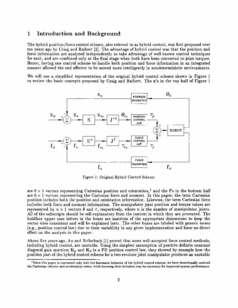
We will use a simplified representation of the original hybrid control scheme shown in Figure 1to review the basic concepts proposed by Craig and Raibert. The x's in the top half of Figure 1

Figure 1: Original Hybrid Control Scheme

are 6 X 1 vectors representing Cartesian position and orientation;' and the f's in the bottom halfare 6 x 1 vectors representing the Cartesian force and moment. In this paper, the term Cartesianposition includes both the position and orientation information. Likewise, the term Cartesian forceincludes both force and moment information. The manipulator joint position and torque values arerepresented by n X 1 vectors f) and T, respectively, where n is the number of manipulator joints.All of the subscripts should be self-explanatory from the context in which they are presented. Theboldface upper case letters in the boxes are matrices of the appropriate dimensions to keep thevector sizes consistent and will be explained later. The other boxes are labeled with generic terms(e.g., position control law) due to their variability in any given implementation and have no directeffect on the analysis in this paper.

About five years ago, An and Hollerbach [1] proved that some well-accepted force control methods,including hybrid control, are unstable. Using the simplest assumption of positive definite constantdiagonal gain matrices K; and Kd in a PD position control law, they showed by example how theposition part of the hybrid control scheme for a two revolute joint manipulator produces an unstable

1 Since this paper is concerned only with the kinematic behavior of the hybrid control scheme, we have intentionally omittedthe Cartesian velocity and acceleration terms, while knowing their inclusion may be necessary for improved system performance.

2

system. Zhang [10] also showed that the hybrid control scheme may become unstable in certainmanipulator configurations using revolute joints. He used a linearized state space approach to showthat the term J-1 S J results in an unstable system for certain manipulator configurations. In bothpapers, only the position part of the hybrid control scheme was examined to reveal a kinematicinstability, which was claimed to be an inherent characteristic of the hybrid control formulation.These results were derived from the equations that are represented by the block diagram shown inFigure 1, that were defined in the architectural framework of the hybrid control scheme given byRaibert and Craig [7].

We will show that the kinematic instability problem attributed to hybrid control is not funda­mental, as the above published works conclude, but the result of an incorrect formulation andimplementation of the hybrid control scheme. It is not clear whether the originators of the hybridcontrol scheme were aware of the subtleties in their approach or the ramifications it would haveon different manipulator kinematics. We intend to show that the hybrid control scheme as stilla very powerful, stable, and robust approach to robot manipulator control. The objective now isto understand and explain why a kinematic instability problem arises in the position part of thehybrid control scheme and to show theoretically why it should never happen. The crux of theproblem has to do with the mapping of Cartesian position errors to joint errors using the inverseof the manipulator Jacobian matrix. The derivation of this equation will be analyzed in the nextsection.

2 The Position Related Equations

For any given task in Cartesian space, the position constraints are separated from the force con­straints by the selection matrix S shown in Figure 1. S is a 6 X 6 diagonal matrix with each diagonalelement being either a one for position control or zero for no position control for each degree offreedom in the Cartesian reference frame of interest. The relevant or selected Cartesian positionerrors are determined as

Xes = S x, (1)

where the Cartesian error vector x, is the difference between the desired and actual Cartesianlocations of the manipulator. The next step is to map the Cartesian error xes to a correspondingjoint error Bes for controlling the manipulator.

The manipulator Jacobian matrix J is the first order approximation for transforming differentialmotions in joint space to differential motions in Cartesian space [6]. The following linearizedrelationship

(2)

is used to map small joint errors Be to their corresponding Cartesian errors X e . A unique inversemapping exists in Equation 2 when J is a square matrix of maximal rank. Under this condition,the joint errors are calculated from the Cartesian errors as

(3)

(4)

By the Craig and Raibert approach for the hybrid control scheme, the selected joint errors aresimply

when using the selected Cartesian errors determined in Equation 1. We will refer to Equation 4 asthe original position solution for Bes .

3

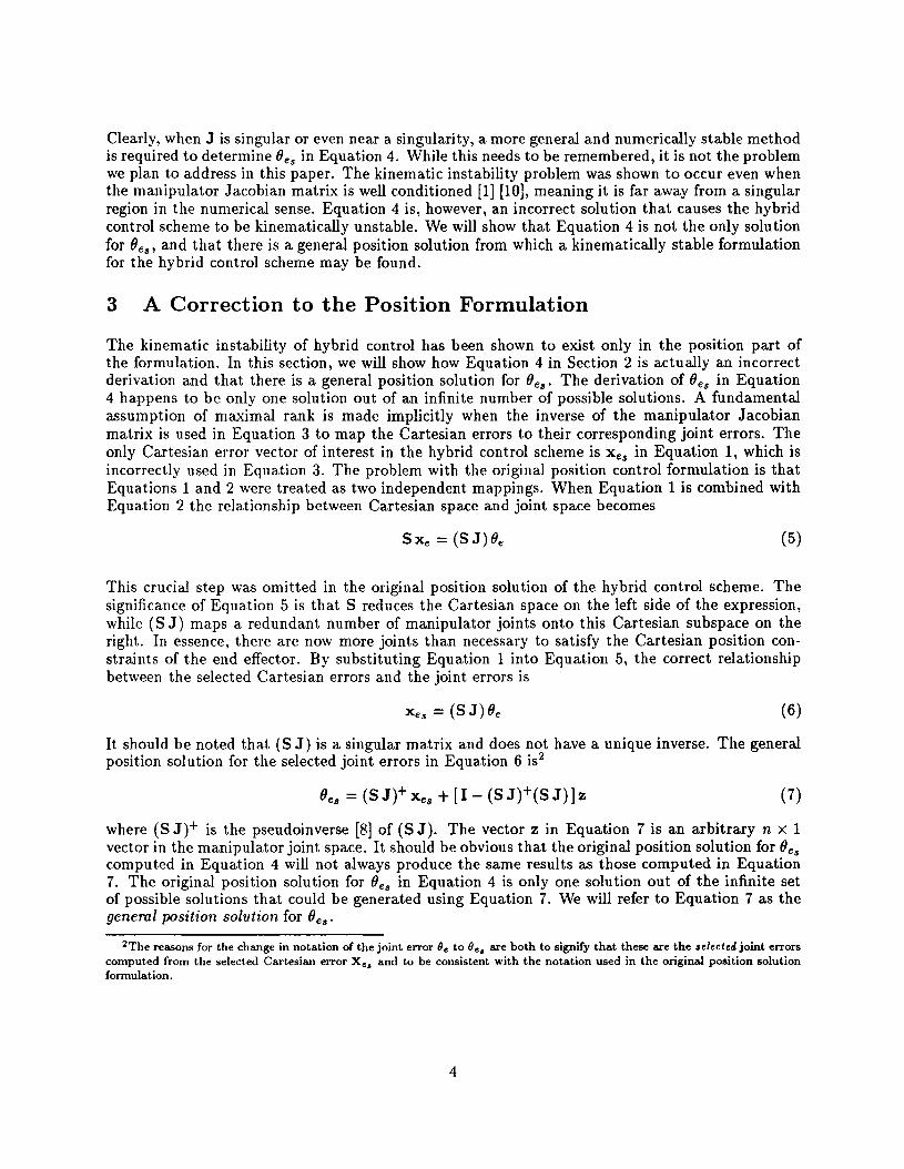
Clearly, when J is singular or even near a singularity, a more general and numerically stable methodis required to determine Bes in Equation 4. While this needs to be remembered, it is not the problemwe plan to address in this paper. The kinematic instability problem was shown to occur even whenthe manipulator Jacobian matrix is well conditioned [1] [10], meaning it is far away from a singularregion in the numerical sense. Equation 4 is, however, an incorrect solution that causes the hybridcontrol scheme to be kinematically unstable. We will show that Equation 4 is not the only solutionfor 8es ' and that there is a general position solution from which a kinematically stable formulationfor the hybrid control scheme may be found.

3 A Correction to the Position Formulation

The kinematic instability of hybrid control has been shown to exist only in the position part ofthe formulation. In this section, we will show how Equation 4 in Section 2 is actually an incorrectderivation and that there is a general position solution for Bes• The derivation of Bes in Equation4 happens to be only one solution out of an infinite number of possible solutions. A fundamentalassumption of maximal rank is made implicitly when the inverse of the manipulator Jacobianmatrix is used in Equation 3 to map the Cartesian errors to their corresponding joint errors. Theonly Cartesian error vector of interest in the hybrid control scheme is xes in Equation 1, which isincorrectly used in Equation 3. The problem with the original position control formulation is thatEquations 1 and 2 were treated as two independent mappings. When Equation 1 is combined withEquation 2 the relationship between Cartesian space and joint space becomes

S'x; = (5J)Be (5)

This crucial step was omitted in the original position solution of the hybrid control scheme. Thesignificance of Equation 5 is that 5 reduces the Cartesian space on the left side of the expression,while (8 J) maps a redundant number of manipulator joints onto this Cartesian subspace on theright. In essence, there are now more joints than necessary to satisfy the Cartesian position con­straints of the end effector. By substituting Equation 1 into Equation 5, the correct relationshipbetween the selected Cartesian errors and the joint errors is

Xes = (5 J) Be (6)

It should be noted that (5 J) is a singular matrix and does not have a unique inverse. The generalposition solution for the selected joint errors in Equation 6 is2

(7)

where (5 J)+ is the pseudoinverse [8] of (5 J). The vector z in Equation 7 is an arbitrary n X 1vector in the manipulator joint space. It should be obvious that the original position solution for Bescomputed in Equation 4 will not always produce the same results as those computed in Equation7. The original position solution for Bes in Equation 4 is only one solution out of the infinite setof possible solutions that could be generated using Equation 7. We will refer to Equation 7 as thegenerol position solution for Bes •

2The reasons for the change in notation of the joint error ee to ee. are both to signify that these are the selected joint errorscomputed from the selected Cartesian error X e• and to be consistent with the notation used in the original position solutionformulation.

4

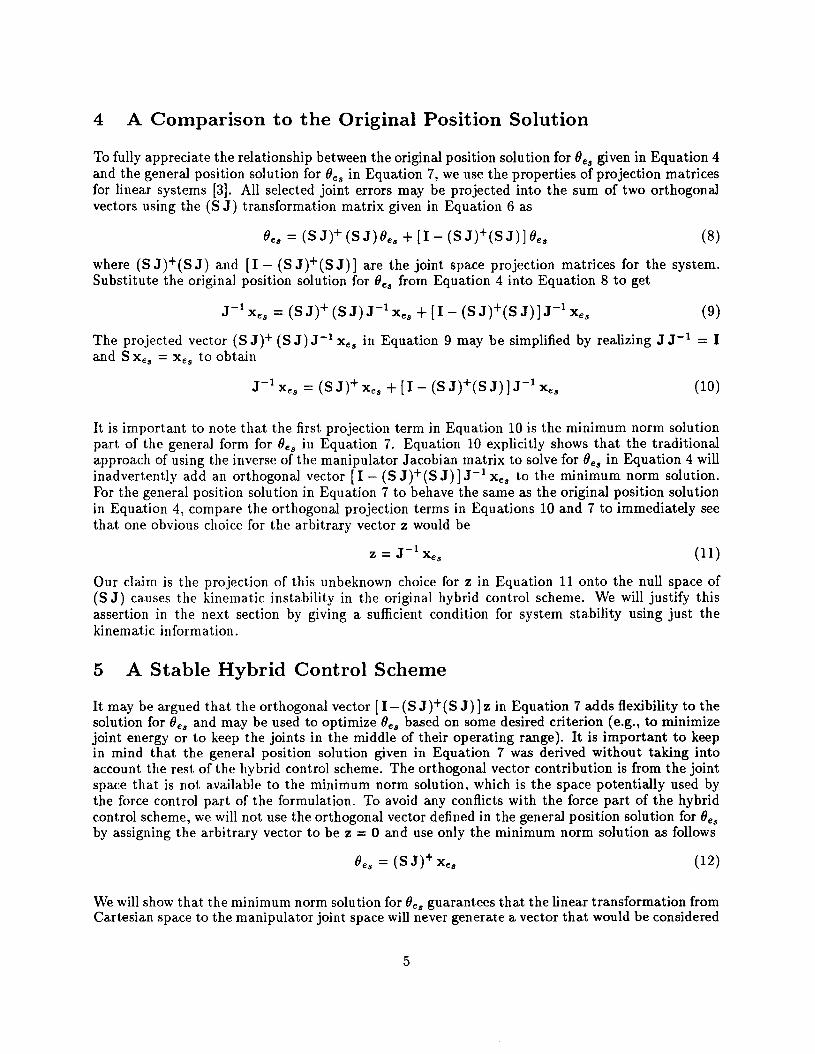
4 A Comparison to the Original Position Solution

To fully appreciate the relationship between the original position solution for Bes given in Equation 4and the general position solution for Bes in Equation 7, we use the properties of projection matricesfor linear systems [3]. All selected joint errors may be projected into the sum of two orthogonalvectors using the (8 J) transformation matrix given in Equation 6 as

(8)

where (8J)+(8J) and [I - (8J)+(8J)] are the joint space projection matrices for the system.Substitute the original position solution for ()es from Equation 4 into Equation 8 to get

(9)

The projected vector (8 J)+ (8 J) J-l Xes in Equation 9 may be simplified by realizing J J-1 = Iand 8 Xes = Xes to obtain

(10)

It is important to note that the first projection term in Equation 10 is the minimum norm solutionpart of the general form for ()es in Equation 7. Equation 10 explicitly shows that the traditionalapproach of using the inverse of the manipulator Jacobian matrix to solve for Bes in Equation 4 willinadvertently add an orthogonal vector [I - (8 J)+(8 J) jJ-l Xes to the minimum norm solution.For the general position solution in Equation 7 to behave the same as the original position solutionin Equation 4, compare the orthogonal projection terms in Equations 10 and 7 to immediately seethat one obvious choice for the arbitrary vector z would be

J - 1Z = Xes (11)

Our claim is the projection of this unbeknown choice for z in Equation 11 onto the null space of(8 J) causes the kinematic instability in the original hybrid control scheme. We will justify thisassertion in the next section by giving a sufficient condition for system stability using just thekinematic information.

5 A Stable Hybrid Control Scheme

It may be argued that the orthogonal vector [1- (8 J)+(8 J)] z in Equation 7 adds flexibility to thesolution for ()es and may be used to optimize ()es based on some desired criterion (e.g., to minimizejoint energy or to keep the joints in the middle of their operating range). It is important to keepin mind that the general position solution given in Equation 7 was derived without taking intoaccount the rest of the hybrid control scheme. The orthogonal vector contribution is from the jointspace that is not available to the minimum norm solution, which is the space potentially used bythe force control part of the formulation. To avoid any conflicts with the force part of the hybridcontrol scheme, we will not use the orthogonal vector defined in the general position solution for Besby assigning the arbitrary vector to be z = 0 and use only the minimum norm solution as follows

(12)

We will show that the minimum norm solution for ()es guarantees that the linear transformation fromCartesian space to the manipulator joint space will never generate a vector that would be considered

5

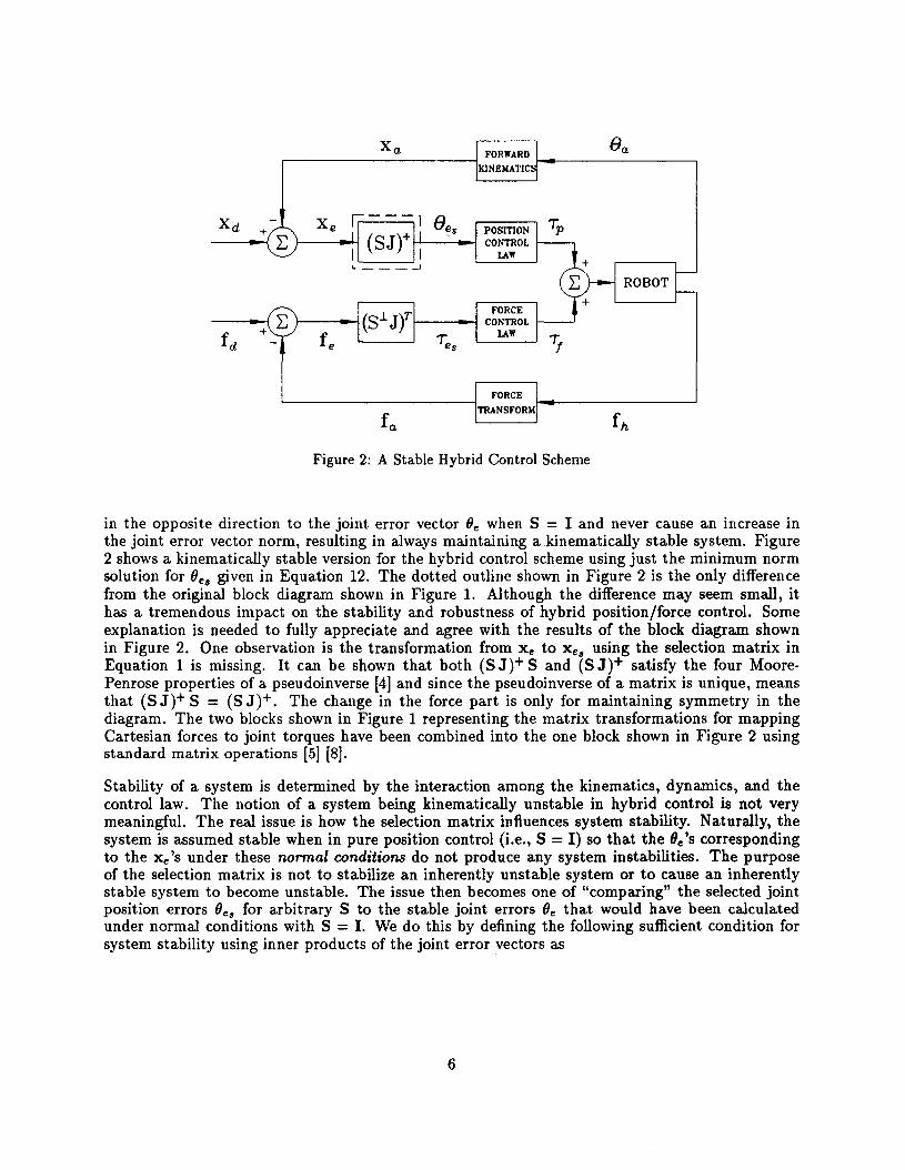
Figure 2: A Stable Hybrid Control Scheme

in the opposite direction to the joint error vector ()e when 8 = I and never cause an increase inthe joint error vector norm, resulting in always maintaining a kinematically stable system. Figure2 shows a kinematically stable version for the hybrid control scheme using just the minimum normsolution for ()es given in Equation 12. The dotted outline shown in Figure 2 is the only differencefrom the original block diagram shown in Figure 1. Although the difference may seem small, ithas a tremendous impact on the stability and robustness of hybrid position/force control. Someexplanation is needed to fully appreciate and agree with the results of the block diagram shownin Figure 2. One observation is the transformation from x, to xes using the selection matrix inEquation 1 is missing. It can be shown that both (8 J)+ 8 and (8 J)+ satisfy the four Moore­Penrose properties of a pseudoinverse [4] and since the pseudoinverse of a matrix is unique, meansthat (8 J)+ 8 = (8 J)+. The change in the force part is only for maintaining symmetry in thediagram. The two blocks shown in Figure 1 representing the matrix transformations for mappingCartesian forces to joint torques have been combined into the one block shown in Figure 2 usingstandard matrix operations [5] [8].

Stability of a system is determined by the interaction among the kinematics, dynamics, and thecontrol law. The notion of a system being kinematically unstable in hybrid control is not verymeaningful. The real issue is how the selection matrix influences system stability. Naturally, thesystem is assumed stable when in pure position control (i.e., S =I) so that the Be's correspondingto the xe's under these normal conditions do not produce any system instabilities. The purposeof the selection matrix is not to stabilize an inherently unstable system or to cause an inherentlystable system to become unstable. The issue then becomes one of "comparing" the selected jointposition errors ()es for arbitrary 8 to the stable joint errors ()e that would have been calculatedunder normal conditions with 8 = I. We do this by defining the following sufficient condition forsystem stability using inner products of the joint error vectors as

6

Sufficient Condition for System Stability:

(13)

It is important to note that both ()e and ()es are computed using the same Cartesian position errorX e , making any solution for ()es always related to ()e' The lower bound in Equation 13 does notallow the projection of ()es onto ()e be in the opposite direction of Be, thereby eliminating anypotentially unstable conditions of introducing positive feedback into the system. The upper boundin Equation 13 restricts the projection of ()es onto ()e to be no larger than ()e, so that the end effectorwill not overshoot its destinations and cause uncontrollable system oscillations. The system maystill be stable when the value of ()eT ()es is outside the bounds given in Equation 13; determininghow far outside the bounds before the system becomes unstable is not straightforward. We willshow in the next section a situation where the lower bound in Equation 13 may become negativeand still maintain a stable system, reinforcing the fact that Equation 13 is only a sufficient and nota necessary condition for stability.

To determine the relationship between ()e and ()es for the position control formulation shown inFigure 2, we combine Equation 12 with Equation 6 to get

(14)

Since (S J)+(S J) is a projection matrix [3], it satisfies the definition of a positive semidefinitematrix [8], meaning the following quadratic expression

(15)

(16)

is true for all vectors ()e' When ()es in Equation 14 is substituted into Equation 13, the innerproduct is exactly Equation 15 and hence, the minimum norm solution for ()es will always satisfythe lower bound in Equation 13. Another property of a projection matrix is that the norm of aprojected vector is bounded by the norm of the original vector [3], meaning the norm of (Jes givenin Equation 14 is bounded by

and so, the upper bound in Equation 13 is also satisfied for all ()e when using the minimum normsolution for ()es' This proves that the minimum norm solution for ()es in Equation 12 will alwayssatisfy the sufficient condition for system stability as defined in Equation 13.

6 A Test Case: The An and Hollerbach Example

In the original hybrid control formulation, the relationship between (Je and (Jes is easily determinedby combining Equations 4, 1, and 2 to get

(17)

An and Hollerbach [1] showed by example that the position part of the system could becomeunstable and that the cause was somehow related to the interaction between the kinematic J-l S Jtransformation matrix and the system inertia matrix. They used a linear state space model ofthe position part of the system to test for the instability by doing a root locus plot of varyingmanipulator configurations. We argue that it is the J-1 S J term that causes the system poles tomigrate into the unstable right half plane for various end effector motions.

7

(~8)

By using the same example, we will show that the J-l S J term is clearly responsible for causingan unstable system when applying the sufficient condition test in Equation 13. In Case 2 of theirpaper, S = diag[O,l] and the Jacobian matrix for the two revolute joint manipulator was given as

J = [ -It 81 - 12 8 12 -12 8 12 ]

It Cl +12 C12 12 C12

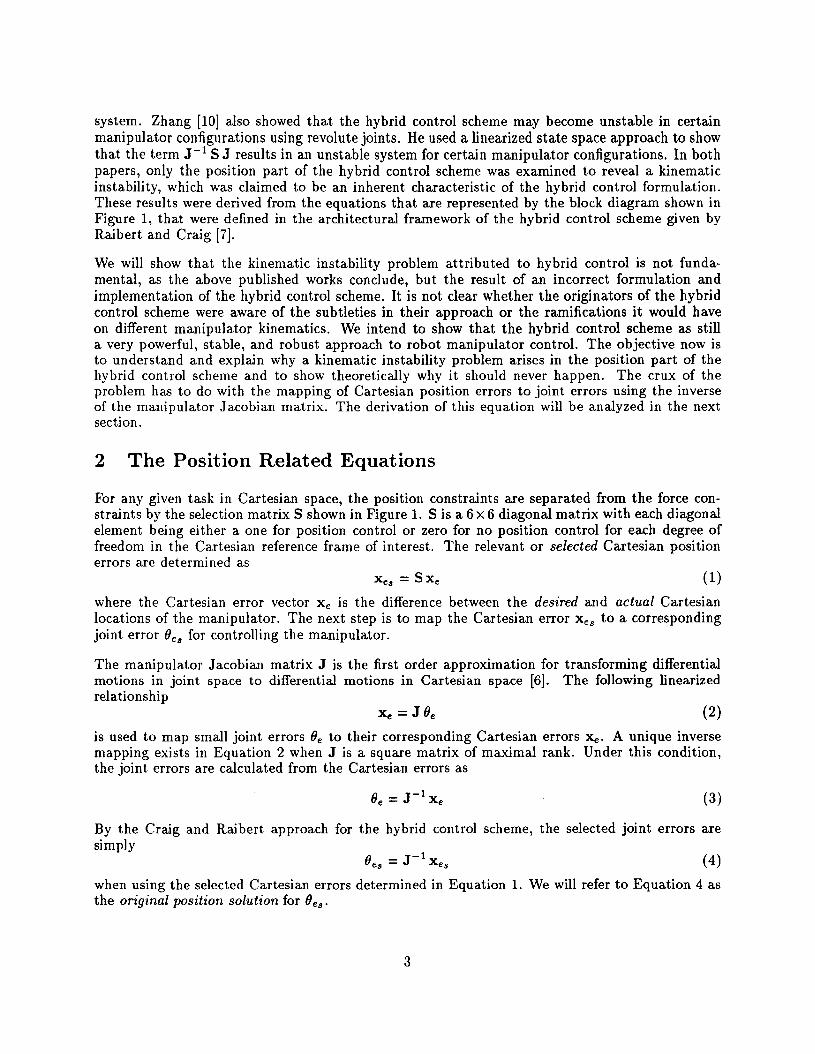
where 8i = sin(Oi), Ci = COS(Oi), 812 = sin(OI + 82 ) , and C12 = COS(OI + 82 ) . The link lengthswere It = 0.462 m and 12 = 0.4445 m. The inner product of Oe with Oell using Equation 17 isOeT (J-l S J) Oe. To test this inner product against the bounds set forth by the sufficient conditionin Equation 13, we will consider the situation where 01 = 0° and 82 varies from -180° to 180° with8e = [0, ±1 JT. A plot of the results is shown in Figure 3. For comparison, a plot of the inner

8, = O·

8. = [o,±lf

/'/.

1

8;(r' SJ) 8. 8;(SJt(SJ) 8.

_-----L __ //----...

<,~

-180·

Figure 3: The Sufficient Stability Test for both Position Formulations

product using the minimum norm solution for 8ell is also shown in Figure 3. It should be clearfrom Figure 3 that the original position solution for 8ell violates the sufficiency condition for systemstability when 118211 ::; 90°. The point marked with an x in Figure 3 was identified by An andHollerbach as the value of 82 where the system transitions from the stable region to the unstableregion. Even though the inner product is negative for the values of 82 from x to 90°, the system isstill stable. The sufficient condition in Equation 13 does not imply the system will be unstable forvalues outside the stated bounds; it only indicates that an unstable situation could occur.

We have included for reference the equations from Section 2.1 of the An and Hollerbach paperregarding the stability analysis of hybrid control. It was stated that the closed-loop system describedas

Me = [ _M-l:p

J-1 S J _M-l ~v J-l S J ] 6x (19)

must have negative real parts for the eigenvalues of the matrix to guarantee local stability at theequilibrium points. The inertia matrix was

(20)

8

(21)

withmn = It +h +m2lt l2c2 + Hml1~ +m21n+ m21~

m12 =m21 =12+ ~m21~ + ~m2lt12c2

m22 = h + ~m21~

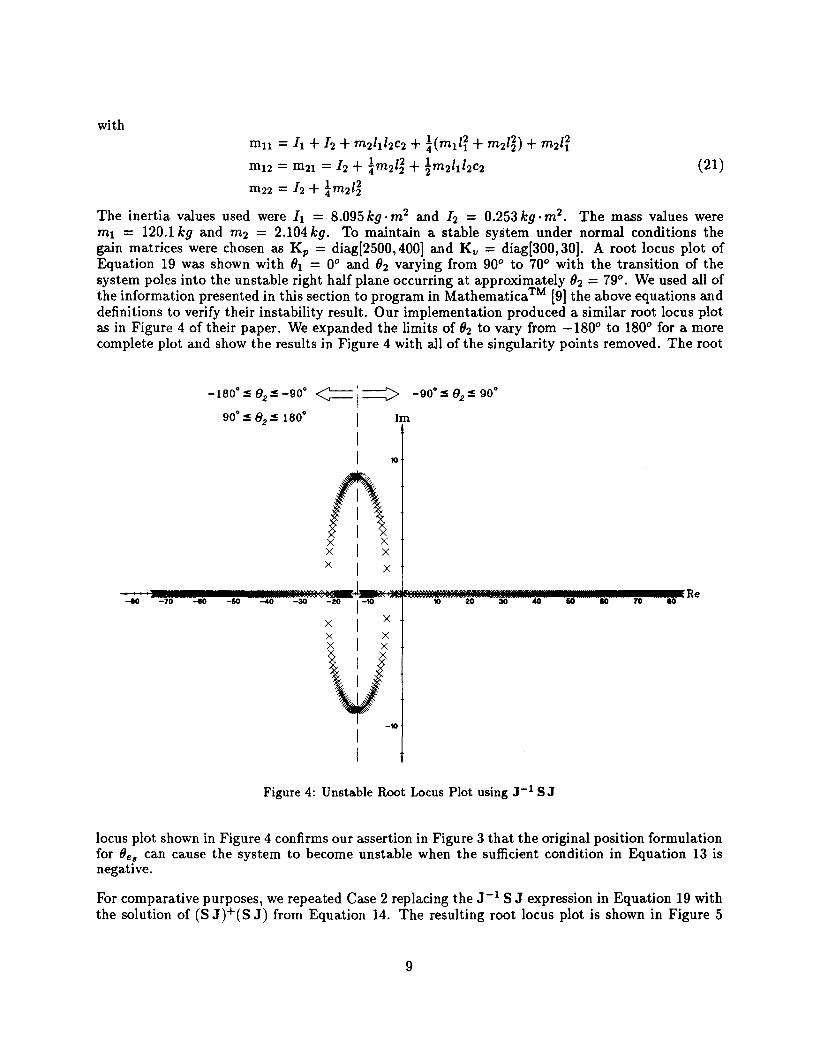
The inertia values used were II = 8.095 kg . m2 and 12 = 0.253 kg· m 2 • The mass values wereml = 120.1 kg and m2 = 2.104 kg. To maintain a stable system under normal conditions thegain matrices were chosen as K p = diag[2500,400] and K, = diag[300, 30]. A root locus plot ofEquation 19 was shown with 01 = 0° and O2 varying from 90° to 70° with the transition of thesystem poles into the unstable right half plane occurring at approximately O2 = 79°. We used all ofthe information presented in this section to program in Mathematica™ [9] the above equations anddefinitions to verify their instability result. Our implementation produced a similar root locus plotas in Figure 4 of their paper. We expanded the limits of O2 to vary from -180° to 180° for a morecomplete plot and show the results in Figure 4 with all of the singularity points removed. The root

-180· ~ 82 ~ -90·

90· ~ 82 ~ 180·

<== i==> _90· ~ 82 ~ 90·

I 1m

II 10

f:\x I XX I X

Re-eo -70 -eo -60 .-.0 -30 -20 ,-10 10 20 30 40 60 10 70 10

X I X

X I X

V-10II

Figure 4: Unstable Root Locus Plot using J-1 S J

locus plot shown in Figure 4 confirms our assertion in Figure 3 that the original position formulationfor Oes can cause the system to become unstable when the sufficient condition in Equation 13 isnegative.

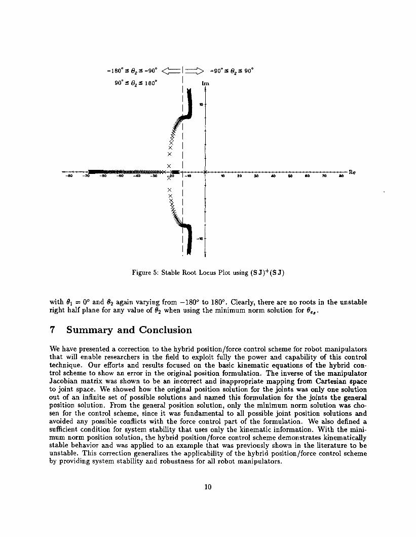
For comparative purposes, we repeated Case 2 replacing the J-l 8 J expression in Equation 19 withthe solution of (8 J)+(8 J) from Equation 14. The resulting root locus plot is shown in Figure 5

9

10

1m

-180· S 82 S -90·

90· S 82 S 180·

~ I==:> -90· S 82 S 90·

IIII

x-ee -70 -80 -50 -~ -30 >to -10

XXX

-10

Figure 5: Stable Root Locus Plot using (S J)+ (S J)

with (Jl = 0° and (J2 again varying from -180° to 180°. Clearly, there are no roots in the unstableright half plane for any value of (J2 when using the minimum norm solution for (Jes.

7 Summary and Conclusion

We have presented a correction to the hybrid position/force control scheme for robot manipulatorsthat will enable researchers in the field to exploit fully the power and capability of this controltechnique. Our efforts and results focused on the basic kinematic equations of the hybrid con­trol scheme to show an error in the original position formulation. The inverse of the manipulatorJacobian matrix was shown to be an incorrect and inappropriate mapping from Cartesian spaceto joint space. We showed how the original position solution for the joints was only one solutionout of an infinite set of possible solutions and named this formulation for the joints the generalposition solution. From the general position solution, only the minimum norm solution was cho­sen for the control scheme, since it was fundamental to all possible joint position solutions andavoided any possible conflicts with the force control part of the formulation. We also defined asufficient condition for system stability that uses only the kinematic information. With the mini­mum norm position solution, the hybrid position/force control scheme demonstrates kinematicallystable behavior and was applied to an example that was previously shown in the literature to beunstable. This correction generalizes the applicability of the hybrid position/force control schemeby providing system stability and robustness for all robot manipulators.

10

8 References

[1] C. H. An and J. M. Hollerbach, "Kinematic Stability Issues in Force Control of Manipulators,"in International Conference on Robotics and Automation, IEEE Robotics and AutomationSociety. Raleigh, North Carolina, pp. 897-903, April 1987.

[2] J. J. Craig and M. H. Raibert, "A Systematic Method of Hybrid Position/Force Control of aManipulator," in Computer Software and Applications Conference, IEEE Computer Society.Chicago, lllinois, pp. 446-451, November 1979.

[3] P. R. Halmos, Finite-Dimensional Vector Spaces. Springer-Verlag New York, Inc., 1974.

[4] B. Noble, "Methods for Computing the Moore-Penrose Generalized Inverse, and Related Mat­ters," in Generalized Inverses and Applications, (M. Z. Nashed, ed.), Academic Press, Inc.,1976. pp. 245-302.

[5] B. Noble and J. W. Daniel, Applied Linear Algebra, Second Edition. Prentice-Hall, Inc., 1977.

[6] R. P. Paul, Robot Manipulators: Mathematics, Programming and Control. Cambridge: MITPress, 1981.

[7] M. H. Raibert and J. J. Craig, "Hybrid Position/Force Control of Manipulators," Journal ofDynamic Systems, Measurement, and Control, Vol. 102. Transactions of the ASME, pp. 126­133, June 1981.

[8] G. Strang, Linear Algebra and Its Applications, Second Edition. Academic Press, Inc., 1980.

[9] S. Wolfram, Mathematica™, A System for Doing Mathematics by Computer. Addison-WesleyPublishing Co., 1988.

[10] H. Zhang, "Kinematic Stability of Robot Manipulators under Force Control," in InternationalConference on Robotics and Automation, IEEE Robotics and Automation Society. Scottsdale,Arizona, pp. 80-85, May 1989.

11