trajectory planning for kinematically … · trajectory planning for kinematically redundant robots...

Journal of Machine Engineering, Vol. 17, No. 3, 2017

Received: 06 January 2017 / Accepted: 17 May 2017 / Published online: 28 September 2017

redundant robots,

trajectory planning,

jacobian matrix, pseudoinverse

Michael WALTHER1*

Andre SEWOHL1

Holger SCHLEGEL1

Reimund NEUGEBAUER1

TRAJECTORY PLANNING FOR KINEMATICALLY REDUNDANT ROBOTS

USING JACOBI MATRIX – AN INDUSTRIAL IMPLEMENTATION

The widespread use of robots in industry contributes significantly to high productivity. Serial 6-axis robots are

used in large quantities, e.g. for assembly or welding. A current emerging trend is the use of robots for classic

tasks of a machine tool like finishing of milled workpieces. For such applications, standard robots are usually

extended by additional axes like linear axes or rotary tilting tables. Therefore, the overall system becomes

kinematically redundant. To be able to calculate the axis quantities via inverse kinematics for a given path,

additional degrees of freedom must be bound. In order to automatically and optimally consider the additional

axis motion a method, using the pseudoinverse of the Jacobian matrix, is discussed. Due to the dependence

of the Jacobi matrix on the robot's current joint position, numerical inaccuracies, which in turn reflect a path

error, are inherent to this method. By feedback control of the path error, in the form of a classic control loop,

the error can be reduced so that a practical implementation on industrial robot controller is possible. In the article

possibilities for parameterisation of the algorithm as well as proof of stability of the closed loop are presented.

The results obtained are verified by a concrete application.

1. INTRODUCTION

For about 40 years, robots in the industrial sector have become indispensable.

The main reason for the use of robots is the automatic execution of a task or service

pursuant to a given program. The automobile industry was a pioneer and still is a supporter

of a widespread use of industrial robots in large numbers. Serial kinematics with six or

fewer axes have mostly been used for applications such as joining, handling or spraying.

In the last decade applications increasingly occur, using robots for flexibilisation

of manufacturing environments. Robots carry out the loading respectively unloading or

the measurement of workpieces on single machine tools or in multi machine concepts.

Another trend, that has become apparent in the recent past, is the exclusive use of robots

(instead of machine tools) in classic manufacturing [1]. This includes processes such as

____________ 1 Chemnitz University of Technology, Faculty of Mechanical Engineering, Professorship for Machine Tools and

Forming Technology, Germany * E-mail: [email protected]

Trajectory Planning for Kinematically Redundant Robots Using Jacobi Matrix – AN Industrial Implementation 25

finishing workpieces by means of grinding or polishing, but also milling, for example, in

wood construction. Also in the aircraft industry in the production of large components [2],

e.g. made of fibre reinforced composites, robots are increasingly used.

With the development of different robotic applications, however, there is a change in

the control of the robots. In the standard six axes applications almost the manufacturer-

specific robot controllers or, in case of simple kinematic chains, motion controllers are used.

In flexible manufacturing environments robots are placed either directly on the machine,

often they are even part of the working space. To control such use cases, robotic solutions

exist as an integration for the computer numerical control (CNC) so that both,

the manufacturing process and the robot application, can be programmed with the same

controller [3]. For the programming and control of robotic systems in production

engineering applications, comparable to machine tools, in most cases the CNC is

exclusively used. In this context many studies address approaches to improve geometric

accuracy of the robot in the processing because of the lower stiffness in comparison to

the machine tool [4,5]. This paper discusses a further aspect using robots in manufacturing

applications: redundancy in the context of kinematic chains. Like mobile and humanoid

kinematic structures, known from the service robotics, robot systems with milling spindles

or additional turn-tilt-tables are mostly kinematically redundant. Further constructions are

known in which robots are completely mounted on a linear axis as shown in Fig. 1.

Fig. 1. Six-axis robot on linear unit [6]

The present paper is devoted to a method for the control technology treatment

of kinematically redundant robots [7], specifically in calculation of the inverse kinematics.

The method is expanded using redundant robots in manufacturing applications. For this

reason, a CNC is applied instead of a classical robot control. In the previous solution,

redundant axis motions were resolved separately. This means, that all six path axes (three

position and three orientation axes) of the robot and all (additionally) redundant axes are

programmed. One aim of the presented method is to program only the six path axes

of the robot and to automatically calculate the additional axes motion in the inverse

kinematics algorithm. Since the method in [7] containing errors, another focus of the paper

26 Michael WALTHER, Andre SEWOHL, Holger SCHLEGEL, Reimund NEUGEBAUER

is to minimize the path error by optimization of the controller parameters, with the aim

of not affecting the positioning accuracy of the robot.

The paper has the following structure: In chapter 0 the term of redundancy in

the context of kinematic chains is specified and subdivided into five different cases.

The differential kinematics for solving redundant axis motion and the stability proof for

the closed loop inverse kinematics are content of chapter 3. In chapter 4 the presented

method is transferred and verified on an application for the production of large workpieces

of fibre reinforced composites. Some selected results for the controller setting and

the resulting path error are presented. The paper closes by summing up the results and

giving an outlook in chapter 5.

2. REDUNDANCY IN THE CONTEXT OF KINEMATIC CHAINS

The degree of kinematic redundancy r is derived from the degree of freedom

of the kinematic chain m (number of joints in case of six axis robot) and from the dimension

me of the end effector movement. Considering the non-redundant case, there are overall five

cases of different determinateness. These are listed below, a more detailed declaration can

be found in [8]:

– Case 1 - General, non-redundant kinematic chain: In the general non-redundant case

the dimension of the joint space m is identical to the dimension of the end effector

space 𝑚𝑒. For each end effector pose, exactly one joint configuration of the robot

(except for the solutions mentioned in Case 2) can be calculated. In the plane case, the

end effector pose is described by three degrees of freedom (2 translations, 1 rotation),

a general spatial movement is described by six degrees of freedom (3 translations, 3

rotations). For a complete description of the end effector pose in space, a serial

kinematics requires six joints.

– Case 2 - Different link constellations, mirror constellations: For almost all kinematic

chains there are different link constellations for one and the same pose of the end

effector (e.g. elbow up and elbow down), and thus multiple but finite solutions for

joint positions can be calculated. The ambiguity in the calculation of the inverse

kinematics can be solved by defining an articulation space for every link constellation

that cannot be left when path interpolation is active.

– Case 3 - Degenerate configuration, singularity: In certain positions of the robot

the dimension of the end effector space 𝑚𝑒 is reduced. Movements in one or more

degrees of freedom are restricted. The difference between the degree of freedom

of the joint space and the order of the reduced end effector space is the degree

of redundancy in the singularity.

– Case 4 – Task redundancy: A further case of redundancy considers relates solely to

the task set for the robot. In case of task redundancy the degree of freedom at the end

effector is greater than it is necessary to handle a task. The degree of task redundancy

𝑟𝑎 is completely independent of the degree of freedom of the joint position space and

only relevant for the control of the end effector. Assuming that the task space is


completely contained in the space of the end effector, the difference between

the dimension of the end effector space 𝑚𝑒 and the task space 𝑚𝑎 describes the degree

of the task redundancy 𝑟𝑎.

– Case 5 - Kinematic redundancy: The case in the relationship between joint and end

effector space, dealt with in the paper, is the kinematic redundancy. If the dimension

of the joint space 𝑚 is larger than the dimension of the end effector space 𝑚𝑒,

the robot is kinematically redundant. There are infinite solutions for the inverse

kinematic problem. The difference between the dimension of the joint space m and

end effector space 𝑚𝑒 describes the degree of kinematic redundancy 𝑟. Furthermore, it

is possible to change the configuration of the kinematic chain without generating

a position or orientation change at the end effector (null space motion).

3. DIFFERENTIAL KINEMATICS

The calculation of motion quantities of a robot is determined by the kinematic

transformation. A distinction is made between direct and inverse kinematic transformation.

The direct kinematics of the robot includes the calculation of robots end effector position

and orientation vector for predetermined joint positon vector of the kinematic chain.

There is always a unique solution. In the inverse case, the ambiguous inverse kinematics

describes the calculation of the joint configuration from a predetermined path at the end

effector. On industrial robot controllers, trigonometric equations are generally used for

the kinematic transformation. For direct kinematics an often used systematic approach is

the Denavit-Hartenberg convention [9]. An efficient closed form solution of the inverse

kinematics for the wide-spread six-axis kinematics can be found in [10].

3.1. NON-REDUNDANT DIFFERENTIAL KINEMATICS

The method of differential kinematics uses the relationship between the vector of joint

velocities �̇� as well as the vector of end-effector velocities �̇� by means of Jacobian matrix

𝐉𝒂(𝐪). This coherence is described in equation (1).

�̇� = 𝐉𝒂(𝐪)�̇� (1)

For the method discussed in the article solely the analytical Jacobian matrix 𝐉𝒂(𝐪) is

used, which offers the possibility to retrieve an orientation description of the end effector in

the Roll-Pitch-Yaw notation. For the general three-dimensional case both, the path vector 𝐱

and the vector of path velocity �̇�, contain three linear and three angular components

(dimension 𝑚𝑒 × 1), see equation (2):

𝐱 = [ 𝑝𝑥 𝑝𝑦 𝑝𝑧 𝑝𝜙 𝑝𝜗 𝑝𝜓 ]𝑇

(2)

�̇� = [ �̇�𝑥 �̇�𝑦 �̇�𝑧 �̇�𝜙 �̇�𝜗 �̇�𝜓 ]𝑇


Corresponding to the joint space, the vectors of robots joint position 𝐪 as well as

velocities �̇� have the dimension 𝑚 × 1 as shown in equation (3). In the normal case

of three-dimensional end effector motion, the kinematic chain requires at least six joints.

In case of kinematic redundancy the number of joints is greater than six.

𝐪 = [ 𝑞1 … 𝑞𝑚 ]𝑇 (3)

�̇� = [ �̇�1 … �̇�𝑚 ]𝑇

From the user perspective, in contrast to equation (1), the inverse kinematic

differential is of greater importance, as in the implementation of an application always

Cartesian path parameters are specified. Depending on the task to be carried out,

the position and orientation of the end effector as well as the path dynamics are specified in

a program. On the assumption that 𝐉𝑎(𝐪) is regular and thus the inverse exists, the vector

of the joint velocities is calculated by:

�̇� = 𝐉𝑎−1(𝐪)�̇� (4)

It is obvious, that equation (4) does not hold in case of kinematic redundancy because

the dimension of vector 𝐪 is greater than six and thus 𝐉𝑎(𝐪) is not square (the inverse 𝐉𝑎−1(𝐪)

does not exist).

For calculating �̇� on an industrial controller in a discrete point of time 𝑡𝑖, the inverse

kinematics is approximated with a difference quotient (5). The time difference between two

calculation steps corresponds to the interpolation clock 𝑡𝐼𝑃𝑂 of the controller.

�̇�(𝑡𝑖) =𝐪(𝑡𝑖) − 𝐪(𝑡𝑖−1)

𝑡𝐼𝑃𝑂

= 𝐉𝑎−1(𝐪(𝑡𝑖−1))

𝐱(𝑡𝑖) − 𝐱(𝑡𝑖−1)

𝑡𝐼𝑃𝑂

(5)

The vector 𝐱(𝑡𝑖) contains the desired path position and orientation at the current time

𝑡𝑖 and 𝐱(𝑡𝑖−1) the corresponding values from the last iteration step 𝑡𝑖−1. By rearranging

equation (5), the current joint position vector 𝐪(𝑡𝑖) can be determined from the desired path

parameters. It dependents on the Jacobian matrix 𝐉𝑎(𝐪(𝑡𝑖−1)) and the joint position 𝐪(𝑡𝑖−1)

of the last iteration step 𝑡𝑖−1. This causes an error in the computation and an extension

of the proposed method discussed in the following section.

3.2. REDUNDANT DIFFERENTIAL KINEMATICS

The calculation of the inverse kinematics in case of redundancy makes the use

of differential algorithms inevitable. The Jacobian matrix in (1) has more rows than columns

and thus is no longer regular. An inversion of the matrix, as in equation (4), is not possible.

There are infinitely many solutions (joint configurations) of the inverse problem for one and

the same pose of the end effector. Therefore it is necessary to bind additional degrees

of freedom in joint space. This can be solved by formulating a linear optimisation problem


with constraints aiming to weight the motion of all single joint axes in equal proportions.

Using the Jacobian transpose 𝐉𝑎𝑇(𝐪), the relationship for the calculation of the Jacobian

pseudoinverse 𝐉𝑎†(𝐪) is described in equation (6). This form is also well known as

Moore-Penrose pseudoinverse and has been introduced independently in [11] and [12].

𝐉𝑎†(𝐪) = 𝐉𝑎

𝑇(𝐪)[𝐉𝑎(𝐪)𝐉𝑎𝑇(𝐪)]−1 (6)

Equivalent to equation (5), a valid solution for the joint configuration can also be

found in case of redundancy.

𝐪(𝑡𝑖) = 𝐉𝑎†(𝐪(𝑡𝑖−1))[𝐱(𝑡𝑖) − 𝐱(𝑡𝑖−1)] + 𝐪(𝑡𝑖−1) (7)

However, there are some practical hitches in implementation of equation (6) on

an industrial robot controller: the dependency of the Jacobian matrix on the joint

configuration and the time discrete integration (Forward Euler method). Both lead to

a computation error. Considering equation (7) at time 𝑡𝑖 only the joint configuration 𝐪(𝑡𝑖−1),

calculated in the last iteration 𝑡𝑖−1, is known. Depending on the sampling rate 𝑡𝐼𝑃𝑂 and

the path velocity �̇�(𝑡𝑖), this leads to considerable errors which are in the magnitude

of robots positioning accuracy. That is the main reason why trigonometric equations are

mostly used to calculate the inverse kinematics on industrial robot controllers. In order to

counteract this, the resulting path error 𝐞(𝑡𝑖) can be included in the calculation

of the inverse kinematics [7]. The error vector 𝐞(𝑡𝑖) contains the deviations between desired

𝐱𝑑𝑒𝑠(𝑡𝑖) and actual 𝐱𝑎𝑐𝑡(𝑡𝑖) path vector at time 𝑡𝑖 (8). The velocity error is obtained by time

derivative of 𝐞(𝑡𝑖):

𝐞(𝑡𝑖) = 𝐱𝑑𝑒𝑠(𝑡𝑖) − 𝐱𝑎𝑐𝑡(𝑡𝑖) = [ 𝑒𝑥 𝑒𝑦 𝑒𝑧 𝑒𝜙 𝑒𝜗 𝑒𝜓]𝑇

(8)

�̇�(𝑡𝑖) = �̇�𝑑𝑒𝑠(𝑡𝑖) − �̇�𝑎𝑐𝑡(𝑡𝑖) = [ �̇�𝑥 �̇�𝑦 �̇�𝑧 �̇�𝜙 �̇�𝜗 �̇�𝜓]𝑇

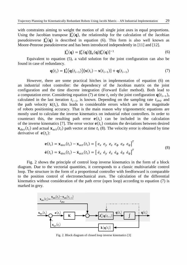
Fig. 2 shows the principle of control loop inverse kinematics in the form of a block

diagram. Due to the vectorial quantities, it corresponds to a classic multivariable control

loop. The structure in the form of a proportional controller with feedforward is comparable

to the position control of electromechanical axes. The calculation of the differential

kinematics without consideration of the path error (open loop) according to equation (7) is

marked in grey.

Fig. 2. Block diagram of closed loop inverse kinematics [3]


The resulting calculation rule for joint position vektor 𝐪(𝑡𝑖) is shown in equation (9).

The diagonal matrix 𝐊 has the dimension 6 × 6 and contains the gain factors in the single

directions of the path vector elements.

𝐪(𝑡𝑖) = 𝐉𝑎†(𝐪(𝑡𝑖−1))[𝐱𝑑𝑒𝑠(𝑡𝑖) − 𝐱𝑑𝑒𝑠(𝑡𝑖−1) + 𝐊𝐞(𝑡𝑖)] + 𝐪(𝑡𝑖−1) (9)

For the implementation of equation (9) on an industrial controller, two difficulties

arise: On the one hand, the factors of the gain matrix 𝐊 have to be parameterised so that

the error between the desired path vector 𝐱𝑑𝑒𝑠(𝑡𝑖) and the resulting path vector 𝐱𝑎𝑐𝑡(𝑡𝑖)

remains as low as possible. On the other hand, it must be guaranteed that the control loop

remains stable in order to generate no unintended end effector movements.

3.3. PARAMETERISATION OF THE GAIN MATRIX

In practice, the parameterisation of the matrix 𝐊 is difficult. General tuning rules are

not known from the literature. The nonlinear controlled system consists essentially

of the Jacobian matrix, which changes in each interpolation cycle. In order to be able to use

the conventional methods of linear control technology, a linearization of the system would

have to take place at a single operating point (path point), with the disadvantage that

the setting for 𝐊 would be optimal only at the operating point or for small changes around

this position. However, in order to obtain a suitable global setting for the path of movement

of the end effector, a metaheuristic optimisation method is used in this article. Advantages

of metaheuristic optimization methods in comparison to analytical approaches are their

applicability even in the case of very complex systems or models (non-linear,

discontinuous) [13].

One possible implementation is the so called simulation-based optimisation.

In general, simulation-based optimisation is a process of finding the global extremum

of an objective function in a defined search space [14]. The optimizer determines a valid

solution of the objective function and submits it to the simulator for evaluation. The main

components of the simulator are a model of the overall system to be examined (in this case

the robot kinematics) and the evaluator for the determined solution.

During the investigations of kinematically redundancy, the simulation-based

optimisation was used to parameterize the gain matrix 𝐊 in equation (9). The error sum

of each path axis over all interpolation cycles corresponds to the selected optimisation

criterion. The optimizer varies the single factors of the matrix 𝐊 with the aim to minimize

the error vector 𝐞 over the complete end effector path motion. The setting results for

the application described in chapter 4 are summarized in Table 1.

3.4. PROOF OF STABILITY USING LYAPUNOV DIRECT METHOD

In addition to the controller setting, it is necessary to prove the stability of control

loop. It has to be guaranteed that the closed control loop with the parameterised controller


shown in Fig. 2 is stable even after the occurrence of a fault. Stability in the context

of system theory means that trajectories do not change too much under small disturbance.

The basic idea of the following proof is the use of Lyapunov second method [15] for

the differential equation of the path error vector 𝐞. The method, which is also called direct

method of Lyapunov, analyses the energetic state of a system. If the energy of a system

decreases, for instance after occurrence of a fault, this also applies to its state variables and

the system is stable.

For proof of stability it is necessary to find a generalized, real-valued differentiable

energy function 𝑉(𝐞(𝑡)) with the following properties (10):

𝑉(𝐞(𝑡)) > 0 für 𝐞(𝑡) ≠ 0 (10)

𝑉(𝐞(𝑡)) = 0 für 𝐞(𝑡) = 0

For proof of stability according to Lyapunov, the change in the energy content

�̇�(𝐞(𝑡)) over time is used. After time differentiation of equation (10) follows the relation:

�̇�(𝐞(𝑡)) =𝜕

𝜕𝐞[𝑉(𝐞(𝑡))]�̇�(𝑡) (11)

The result from the equation (11), specified by the following case distinction (12), can

be used for stability assessment:

�̇�(𝐞(𝑡)) < 0 energy content of the system decreases, so the

state variables also decrease (12)

�̇�(𝐞(𝑡)) ≥ 0 energy content of the system remains constant or

increases, the same applies to the state variables

In the case of the redundant inverse kinematics with Jacobian pseudoinverse a positive

definite and quadratic function of the path error (13) is suitable for 𝑉(𝐞(𝑡)) [16]. If all

the individual gain factors of the matrix 𝐊 are positive, then 𝑉(𝐞(𝑡)) satisfies the properties

(10).

𝑉(𝐞(𝑡)) =1

2𝐞𝑇(𝑡)𝐊𝐞(𝑡) (13)

According to the time derivative in (11) and after the substitution of (8) one obtains.

�̇�(𝐞(𝑡)) = 𝐞𝑇(𝑡)𝐊(�̇�𝑑𝑒𝑠(𝑡) − �̇�𝑎𝑐𝑡(𝑡)) (14)

Furthermore, the actual path velocity �̇�𝑎𝑐𝑡(𝑡) with equation (1) as well as

the calculated joint velocity �̇�(𝑡) by the integration of equation (9) can be replaced (15):


�̇�(𝐞(𝑡)) = 𝐞𝑇(𝑡)𝐊�̇�𝑑𝑒𝑠(𝑡) − 𝐞𝑇(𝑡)𝐊𝐉𝑎𝐉𝑎†(�̇�𝑑𝑒𝑠(𝑡) + 𝐊𝐞(𝑡)) (15)

Under assumption, that the term 𝐉𝑎𝐉𝑎† is equal to the identity matrix, the time variation

time of the energy function (13) is obtained (16):

�̇�(𝐞(𝑡)) = −𝐞𝑇(𝑡)𝐊𝐊𝐞(𝑡) (16)

If matrix 𝐊 is positively definite, the function (16) is negative and satisfies the stability

condition (12). A graphical representation of the function for the application discussed

in section 4.1 is illustrated in Fig. 4.

4. APPLICATION AND RESULTS

4.1. APPLICATION SIX-AXIS ROBOT ON LINEAR AXIS

The plant concept, for which the presented method has been implemented, comprises

an approx. 6 m long motion path for processing an aircraft wing [17]. It includes a KUKA

robot KR500-2, which is mounted on a linear axis with direct drive and can be moved along

the workpiece. The system is mechanically over-determined. The degree of kinematic

redundancy 𝑟, discussed in Case 5, chapter 0, is one.

The desired path is basically planned and programmed in the coordinates of the tool

center point in a computer-aided manufacturing system. The previously available output

corresponds to a program for numerical control (G-code), which includes the Cartesian

position and orientation of the tool head as well as a simple resolution of the redundant axis

motion according to empirical algorithms (e.g. constant velocity along the path).

Describing the end effector motion only with the necessary number of degrees

of freedom and automatically resolving the redundant axis motion is the main objective in

this application. In addition, the path error caused by the use of the differential kinematic

algorithm (9) should be smaller than the positioning accuracy of the robot in order to justify

a practical use on industrial controllers and to guarantee a precise processing operation.

4.2. SELECTED RESULTS

For calculating the inverse kinematics and binding the redundant linear axis motion,

equation (9) is implemented as algorithm. In the first step the determination of the elements

in the gain matrix 𝐊 was carried out empirically. However, this method is very

time-consuming and inaccurate, which excludes practical use. For this reason, the method

of simulation-based optimisation (section 3.3) is used for the controller setting. The single

elements of 𝐊 are varied until the path error is minimal. The settings obtained empirically as

well as by simulation-based optimisation are summarised in Table 1.


Fig. 3 shows the time course of the three position components 𝑒𝑥, 𝑒𝑦 and 𝑒𝑧 of path

error 𝐞. Compared to the results of differential inverse kinematics, the geometric solution

of the controller can be assumed to be ideally zero. Errors in the geometric solution are

mainly results in the limited binary representation of a number (e.g. 16 bit) on the controller.

Table 1. Parameterisation of the gain matrix 𝐊

Empiric Simulation based optimisation

𝐾𝑥 1.00 1.92

𝐾𝑦 1.00 1.84

𝐾𝑧 1.00 1.87

𝐾𝜙 10.00 11.09

𝐾𝜗 2.00 5.98

𝐾𝜓 2.00 2.27

By comparing the results of the empirical setting and the simulation-based

optimisation, it becomes clear that the extreme values of the optimised setting are only half

as large. However, the inaccuracy caused by the use of differential algorithms is far below

the positioning accuracy of a robot. A practical use of the presented algorithm on

an industrial controller becomes possible. Similar statements can be made for the orientation

errors. A further reduction of the error can be achieved by defining error limits for the entire

path [18]. However, due to the limited computing time of an industrial control, this was

initially neglected during implementation.

Fig. 3. Time course of the path error 𝐞 - Position of the tool center point

Another aspect discussed in the paper is the proof of stability. Fig. 4 shows the time

course of function �̇�(𝐞(𝑡)) for the optimised settings from Table 1. It is obvious that

the time derivative of the energy content is negative along whole path and the system in

Fig. 2 is Lyapunov stable. This is of great importance, especially for practical use, for

example in case of external disturbances.

Empiric settingTrigonometric solution Optimised settingTime [s]

10 20 7060504030

0

0

0

10

10

20

20

30

30

40

40

50

50 60

60 70

70

0.00E + 0

-1.00E - 4

-2.00E - 4

-1.50E - 4

-5 .00E - 5

-2.00E - 4

-1.00E - 4

0.00E + 0

-2 .50E - 4

e [

mm

]x

e [

mm

]y

e [

mm

]z


Fig. 4. Time derivative of Lyapunov function �̇�(𝐞(𝑡)) for optimised setting

5. CONCLUSION AND SUMMARY

The present paper covers with the trajectory planning of redundant robotic systems on

industrial controllers. A differential algorithm, based on the Jacobian pseudoinverse, is

presented. One focus of the work is the parameterisation of the gain matrix 𝐊 in order to

allow including the errors from the calculation of the inverse kinematics. The use

of a metaheuristic optimisation method helps finding an useful setting. It is also shown that

closed loop inverse kinematics with Jacobian pseudoinverse is stable for a positive definite

gain matrix 𝐊. In the described application, it becomes clear that it is possible to minimize

the error such that the differential inverse kinematics can be used for the automatic

resolution of redundant axis movements on an industrial control.

In the current work the method is modified for additional calculating in the preparation

of a numerical control. In the preparation of the trajectory planning the path dynamics is

estimated. At this point of time no physical path velocity exists which is problematically

using equation (9). In addition, a method for deriving a general tuning rule for the matrix 𝐊

is to be developed from the existing results.

REFERENCES

[1] DENKENA B., BRÜNING J., LEPPER T., 2015, Innovative Zerspanung mit Industrierobotern Qualitäts- und

Produktivitätssteigerung mittels ganzheitlicher Prozessbetrachtung, ZWF Zeitschrift für wirtschaftlichen

Fabrikbetrieb, 2015 (09).

[2] BORRMANN C., 2016, Adaptive Montageprozesse für CFK-Großstrukturen mittels Offline-Programmierung von

Industrierobotern, Dissertation, TU Hamburg-Harburg, Hamburg.

[3] KIEF H.B., ROSCHIWAL H.A., 2015, CNC-Handbuch 2015/16, München, Hanser, 766.

[4] RÖSCH O., 2014, Steigerung der Arbeitsgenauigkeit bei der Fräsbearbeitung metallischer Werkstoffe mit

Industrierobotern, Dissertation, TU München.

0.00E + 0

-1.00E - 4

-2.00E - 40 10

-1.50E - 4

-5.00E - 5

-2.50E - 4

0.00E + 0

-1.00E - 4

-2.00E - 4

0 10

100

e Xim

mm

e Xim

mm

e Xim

mm

0 10 20 30 40 50 60 70

0.00

-0.16

-0.12

-0.10

-0.08

-0.06

-0.04

-0.02

-0.14

Time [s]

V(e

) [m

m]


[5] SCHNEIDER U., DRUST M., ANSALONI M., LEHMANN C., PELLICCIARI M., LEALI F., GUNNINK J. W.,

VERL A., 2016, Improving robotic machining accuracy through experimental error investigation and modular

compensation, The International Journal of Advanced Manufacturing Technology, 85/1-4, 3-15.

[6] Kuka Roboter GmbH, Lineareinheit KL 3000, http://www.kuka-robotics.com/germany/de/products/addons/

linearunits/PA_KL3000_Detail.htm (as consulted on-line on 22.12.2016).

[7] CHIACCHIO P., CHIAVERINI S., SCIAVICCO L., SICILIANO B., 1991, Closed-loop inverse kinematics

schemes for constrained redundant manipulators with task space augmentation and task priority strategy. In: Int.

J. Rob. Res. 10, July, 4, 410-425.

[8] CONKUR, E.S., BUCKINGHAM, R., 1997, Clarifying the definition of redundancy as used in robotics, Robotica

15, 583-586.

[9] HARTENBERG R.S., DENAVIT J., 1964, Kinematic synthesis of linkages, McGraw-Hill, New York, 435.

[10] PIEPER D.L., 1968, The kinematics of manipulators under computer control, Stanford University, dissertation,

http://www.dtic.mil/dtic/tr/fulltext/u2/680036.pdf, online–resource p. 174 (downloaded on 11.01.2016).

[11] MOORE E.H., 1920, On the reciprocal of the general algebraic matrix, Bulletin of the American Mathematical

Society, 26, 394-395.

[12] PENROSE R., 1955, A generalized inverse for matrices, Proceedings of the Cambridge Philosophical Society, 51,

406-413.

[13] MOHAN C., DEEP K., 2009, Optimization Techniques, Tunbridge Wells, New Age Science Limited.

[14] HIPP, K., HELLMICH, A., SCHLEGEL, H., DROSSEL, W.-G., 2014, June, Criteria for controller

parameterization in the frequency domain by simulation based optimization, 14th Mechatronics Forum

International Conference, Karlstad, Sweden.

[15] LYAPUNOV A.M., 1995, The general problem of the stability of motion, Automatica, 3/2, 353-356, London,

ISBN 978-0-7484-0062-1.

[16] SCIAVICCO L., SICILIANO B., 2005, Modelling and control of robot manipulators, Advanced Textbooks in

Control and Signal Processing, 2 ed., Springer, XXIII, 378.

[17] WALTHER M., HAMM C., HIPP K., NEUGEBAUER R., TAUCHMANN S., 2014, Optimale Ausnutzung von

Achsredundanzen bei der Bahnplanung von Robotern, SPS/IPC/DRIVES, Nürnberg, VDE Verlag GmbH.

[18] WALTHER M., HIPP K., SCHLEGEL H., NEUGEBAUER R., 2015, Jacobi-Matrix basierte Bahnplanung für

Roboter mit Achsredundanzen, Scientific Reports, Journal of the University of Applied Sciences Mittweida, 2,

ISSN 1437-7624.

http://www.dtic.mil/dtic/tr/fulltext/u2/680036.pdf

trajectory planning for kinematically … · trajectory planning for kinematically redundant robots...

Documents