a keynesian macroeconomic model with new-classical ...lrazzolini/gr1988.pdfa keynesian macroeconomic...

A Keynesian Macroeconomic Model with New-Classical Econometric Properties*

JAMES PEERY COVER

University of Alabama Tuscaloosa, Alabama

I. Introduction

The development of New-Classical macroeconomic models with policy implications radically different from Keynesian models calls for econometric tests which can determine with which type of model the available data is most consistent. At least two types of tests have been proposed. Each one is based on the presumption that New-Classical models imply certain restrictions on estimated coefficients in reduced-form equations that are not implied by Keynesian models. The purpose of this paper is to demonstrate that there is a plausible Keynesian model which is consistent with two testable restrictions implied by New-Classical models.' The two restrictions are: (1) the argument that in New-Classical models the nominal quantity of money and other nominal variables do not

Granger-cause output and other real variables, while this is not the case in Keynesian models;2 and (2) the argument that New-Classical models imply cross-equation constraints which do not hold in Keynesian models.3

The results of this paper are important for two reasons. Firstly, proponents [10, 401; 17, 403] of the above-mentioned tests believe that the rejection of the "New-Classical" restrictions is not evidence against the New-Classical structure in favor of the Keynesian structure. That is, there may be New-Classical models in which the restrictions do not apply. But at the same time McCallum [110] and Sargent [17] both believe that acceptance of these restrictions is clear evidence in favor of the New-Classical structure because such results, "would be very difficult to explain according to Keynesian macroeconomic models" [17, 403].

*The author is grateful to the University of Alabama Research Grants Committee for a grant-in-aid received in support of this research. The author thanks David Schutte, Matthew J. Cushing and Donald Hooks for helpful comments on an earlier draft. The author is responsible for all remaining errors and omissions.

1. In addition to the two restrictions discussed below one may be tempted to bring up the sort of restriction emphasized by Barro [1; 2] in which he estimates the expected money supply and tests the hypotheses that the expected component of the money supply does not affect output, while the unexpected part does. However, by examining how Barro's results differ from those of Mishkin [12; 13], and McCallum's [7] analysis and results, it is obvious that the results of tests of this restriction are extremely sensitive to the manner in which expected money is defined. (To be more to the point, and more in line with McCallum's analysis, the results are sensitive to the variables included in the information set.) The two tests emphasized below do not suffer from this problem. Furthermore, such a restriction is in principle consistent with the restriction that nominal variables do not Granger-cause real variables.

2. See Sargent [15; 16; 17] and McCallum [9] for attempts to implement this test and arguments for its use. 3. See McCallum [10] for arguments for the use of this test.

831

832 James Peery Cover

Secondly, proponents [6] of the increasingly popular "real" theories of business cycles have used the failure of money to Granger-cause output as evidence in favor of such real theories and as evidence against alternate theories. Below it is demonstrated that it is actually quite easy to derive these testable restrictions from a Keynesian macroeconomic model.

The Keynesian model presented below produces results different from other Keynesian models because it presumes that monetary policy is implemented in a manner which causes

expected aggregate demand to equal expected aggregate supply. In a disequilibrium Keynesian model aggregate demand can differ from aggregate supply because prices do not adjust rapidly enough to equate the two continuously.4 Keynesians presume that in the real world the Walrasian auctioneer does not call out arrays of prices while time stands still. Rather economic actors must

consciously decide whether to bid prices upwards or downwards. This takes time! Even if ex-

pectations are rational, there is no guarantee that markets will continuously clear. However, in such a world, if policy-makers have a working knowledge of how prices are adjusting towards the equilibrium price level, then they may be able to implement a monetary policy that causes the expected value of aggregate demand to equal the expected value of aggregate supply. If

disequilibriums between aggregate demand and aggregate supply are responsible for important fluctuations in output, then in order for a policy to be optimal it must cause expected aggregate demand to equal expected aggregate supply.

If it is assumed that the policy implemented in a Keynesian model is one which causes

expected aggregate demand to equal expected aggregate supply, then any differences between realized aggregate demand and realized aggregate supply are random. Even though policy is help- ing to keep the economy close to equilibrium, and is therefore affecting output, econometrically it appears that policy is having no effect on output; that nominal variables do not Granger-cause real variables; and that the cross-equation constraints associated with New-Classical models hold.

Consideration of this type of policy within a Keynesian model has at least one other interest-

ing implication-the finding that the Lucas aggregate-supply equation is not necessary in order to find econometrically that unexpected changes in the money supply affect output, while expected changes do not.

The reader who believes that consideration of such a policy is not empirically relevant is

urged to withhold judgment until reading the final section. Section II presents a standard New-Classical model and demonstrates how it implies the

above two testable restrictions. Section III introduces a form of price stickiness and explains why it is generally believed that Keynesian models are inconsistent with the above two testable restrictions. Section IV changes the nature of monetary policy in the Keynesian model from an

arbitrary feedback rule to the policy that causes expected aggregate demand to equal expected aggregate supply. It is then demonstrated that in a Keynesian model in which policy makers

implement this sort of optimal policy, the above two testable restrictions also hold. Section V

points out that the Lucas aggregate-supply equation is unnecessary for these results, while section VI offers some supporting empirical evidence and a conclusion.

4. For this view of Keynesian economics see Patinkin [14, 313-348], Clower [4], and Barro and Grossman [3]. Note that the argument for price-stickiness employed by Patinkin and used here does not depend upon the existence

of long-term contracts, rather it rests on the presumption that the Walrasian auctioneer, i.e., the free, perfectly competitive market, does not adjust while time stands still. Whether one accepts this argument or not does not affect the result of this paper, which is that proposed empirical tests are not capable of distinguishing New-Classical models from a model with price-level stickiness.

A KEYNESIAN MODEL WITH NEW-CLASSICAL PROPERTIES 833

II. A New-Classical Model

The New-Classical model employed here is a variant of those employed by Sargent [15], Sargent and Wallace [18], and McCallum [11]. It consists of the following equations:

Yt = bo + birt - blEt-l(Pt+l -Pt) + Yt, bl

< 0; (1)

mt - pt = co + cirt + C2Yt + "t, C1 < O, C2 > 0; (2)

Yt = ao + alyt-1 + a2(Pt - Et-lpt) + ut, al, a2 > 0; (3)

mt = xo -

xlmt-1 -

x2mt-2 - x3Yt-1 I t, Xi > 0. (4)

Yt , m,, and Pt respectively are the logrithms of output, the nominal quantity of money, and the price level, while r, is the nominal rate of interest. y,, e,, rt, and ut are serially and mutually uncorrelated disturbances. Et- denotes the mathematical expectation of the variable on which it operates, conditional on information available at the end of period t - 1. Equation (1) is an IS curve; equation (2) is an LM curve; equation (3) is a Lucas-type aggregate supply equation; and equation (4) is a money-supply feedback rule. Although one can quarrel with the above

specification, reasonable modifications do not affect the thesis of this paper (which is to show that a particular, reasonable Keynesian model implies the same testable constraints as the above

model). The solution for output in the above model is:

y, = ao + aly,-1 + [azcy, + a2b!(e, - i,)

+ bIu,] B, (5)

where B = bl + cla2 + czbla2 < 0. If equation (4) is solved for E, and the result is inserted into

(5), the result is

y,=ao - (az2bxo B) + [a, + (a2bix3 B)]y,-l+

(az2bIB)[m, -+ x1m,-1 +

x2zm,-2 +

[a2zcy - az2br1, +

blu,]l B. (6)

Equation (5) clearly implies that the above model is consistent with the proposition that

only unexpected changes in the money supply affect the level of output. This follows because the

disturbance, c,, is the only term from the money-supply feedback rule that appears in equation (5). Equation (5) also implies that output, y,, is not Granger-caused by the money supply and the

price level. This follows because E,, y,, r9,. and u, are orthogonal to past values of the money supply and the price level. This is the first testable implication of the New-Classical model.

Equations (6) and (4) together imply that the estimated coefficients on past values of money in a regression equation for output are proportional to those in a regression equation for money. Here the proportion is (a2b /B). This simple-proportionality, cross-equation constraint is the second

testable implication of the above model.

III. A Keynesian Model Inconsistent with the Two Restrictions

One assumption implicit in the above model is that the price level adjusts so that aggregate demand always equals aggregate supply. Many Keynesians traditionally have assumed that prices adjust


price level

aggregate supply

t-1

AD'

t= p* + (1- )t1 ADt- 1

AD

output

Yt Y

Figure 1

sluggishly. Following McCallum [8], one way in which the above model can be modified so that it is in principle consistent with this Keynesian presumption is to assume that Pt* is the price level at which aggregate demand equals aggregate supply, but the price level which actually prevails during period t is defined by5

Pt = Ap* + (1 - A)pt-1, O < A < 1. (7)

If aggregate demand is less than aggregate supply (Pt > Pt),

then it is assumed output equals aggregate demand. If aggregate demand is greater than or equal to aggregate supply (Pt < Pt), then it is assumed that output equals aggregate supply.

Figure 1 illustrates the workings of this price-adjustment equation in a model with a fixed, vertical, aggregate-supply curve. Suppose that during period t - 1 the economy is in equilibrium at price level Pt -1 and output y*. If the long-run, aggregate-supply curve is fixed over time at y *, and there is a decrease in aggregate demand from ADt -1 to ADt during period t, output declines to yt because the price level does not decrease all the way to

pt*. If the aggregate demand curve

remains at ADt and the aggregate supply curve remains at y* during future periods, then the price level gradually declines toward

pt* and output gradually increases toward y*. (If the aggregate

demand curve shifts to AD ' during period t, then output would remain at y*, while the price level

gradually increases to p'.) As the above discussion implies, and has been rigorously demonstrated by McCallum [8], if

output always equals aggregate supply, then the testable restrictions of New-Classical models will continue to obtain. But it should be obvious that such restrictions will not hold in general under the Keynesian assumption that output equals aggregate demand. However, as is demonstrated in the next section, under a reasonably optimal policy the restrictions continue to hold even if output equals aggregate demand.

5. The particular type of price stickiness that exists is not important for the results of this paper, so long as it is a type that allows policy to affect aggregate demand. The results below differ from McCallum's [8] because he assumes

output always equals aggregate supply, while here it is assumed that if aggregate demand is less than aggregate supply, then output equals aggregate demand. McCallum's assumption is impossible in an economy in which a large part of output consists of services. Furthermore, the assumption that output equals aggregate demand whenever aggregate demand is less than aggregate supply is consistent with Patinkin [14], Barro and Grossman [3], and many textbook treatments of

Keynesian macroeconomics.


price level

s E ys Y -1 t -1it

Ep=P -E p

E t-ltt t-- I

I t-i

I output t -1 EYt =a01 t o -

Figure 2

IV. Rational Policy in a Keynesian Model

In New-Classical models demand-side disturbances cause fluctuations in output only because of the effects on aggregate supply of unexpected changes in the price level. Disequilibrium Key- nesians in principle need not disagree with the existence of such an effect. Be that as it may, disequilibrium Keynesians emphasize that demand-side disturbances may affect output because of price-level stickiness. In particular, if there is a decrease in aggregate demand, price-level stickiness prevents the price level from declining to the level at which aggregate demand equals aggregate supply. As a result, output declines to the level of aggregate demand.6

If price-level stickiness is a major cause of output fluctuations, then a rational policy maker would implement policy in a manner such that there is no need for the price level to change. (The exact policy depends on the type of price stickiness that exists. For example, if the rate of inflation is sticky, then the proper policy is one which does not require the rate of inflation to

change.) Consider the model represented by equations (1)-(3) and (7). In Figure 2 the curve labeled

yt-1 represents aggregate demand during period t - 1, while the curve labeled Yf_1 represents aggregate supply during period t - 1. It is assumed for purposes of discussion that aggregate demand equals aggregate supply during period t - 1, although in general this is not necessarily the case in a Keynesian model.

Although policy-makers cannot prevent there from being a disequilibrium between aggregate demand and aggregate supply during period t, they can implement a policy which causes the

expected value of aggregate demand to equal the expected value of aggregate supply. But as

long as (7) holds, this can only be the case if the expected value of the equilibrium price level,

pt*, is

Pt-1. Hence, in Figure 2 the optimal policy, or the policy which minimizes the expected disequilibrium between aggregate demand and aggregate supply is one which causes the expected, aggregate-demand curve for period t, Et-lyd, to intersect the expected, aggregate-supply curve,

Et-lYt, at Pt-1. It is concluded that in the model consisting of equations (1)-(3) and (7), an

optimal policy must be one which causes Et- iP = Pt -1. If economic actors are certain that such a policy is going to be maintained, then the expected

rate of inflation is zero, or Et -l (Pt +1 - Pt) = 0. Hence the model becomes

6. See Patinkin [14, 316-24] and the above discussion of Figure 1.


Pt = Apt* + (1 - A)pt,-1;

(7)

td = bo + birt + Yt; (8)

mt - Pt = co + Clrt + C2yt + 71t; (9)

yt = ao + alyt-1 + a2(pt - Et-lPt) + ut; (10)

Et- IPt = Et- Ip; = Pt -1. (11)

In equation (9) Yt equals yd iif output equals aggregate demand; while it equals yt

if output equals aggregate supply. There are several ways that policy-makers can insure that (11) holds. Since for present purposes it does not matter how this is done, it is assumed that the monetary authority tries to set the money supply at the level which causes (11) to hold.

Applying the expectations operator to (9) and rearranging yields

Et-imt = Et-lp, + co + clEt,-rt

+ C2Et-lYt. (12)

Applying the expectations operator to (8) and solving for Et - Irt yields

Et-lrt = -(bo/bl) + (1/bl)Et-ly,.

(13)

Substituting (13) into (12) yields

Et-lmt = Et-lpt + [(cobl - bocl)/b,]

+ [(C2bl + cl)/bl]Et-lyt. (14)

Recall that so long as Et -Pt = Pt-1, then Et -I y =

Et-lyt

= ao + alyt-1. Making these sub- stitutions yields

Et-imt = [c2ao + co + cl(ao - bo)/bl] + pt-1 + (al/bi)(c2bl + cl)yt-1. (15)

Equation (15) implies that the following money-supply rule will cause (11) to hold and cause expected aggregate demand to equal expected aggregate supply:

mt = [c2ao + co + cl(ao - bo)/bl] + pt-1 + (al/bi)(c2bl + cl)yt-1 + Et. (16)

If the model consisting of equations (7)-(10) and (16) is solved, the solutions for the price level, aggregate demand and aggregate supply are as follows:

Pt =Pt- + (A/B)[city

+ bi(et - t) - (c1 + C2bi)ut]; (17)

Yd =ao + alyt-1 + (blA/B)ut +

{[az(cl + C2bl) + bil(1 - A)][bl(et - rt,) + clyt]/[B(cl + Czbl)]}; (18)

YF=ao + alyt-1 + {Aa2Cly, + Aa2bl(et - rlt)+ [az(1 - A)(Cl + C2bi) + bi ]ut } /B; (19)

where B = bl + a2cl + a2c2bl < 0.

Notice from equations (17)-(19) that the conditional expectation of the price level equals

Pt-1, while the conditional expectations of both aggregate demand and aggregate supply equal ao + alyt -1. Finally, note that if A = 1, then y/ =

yts. These results imply that, under the policy


considered here, output is not Granger-caused by any nominal variables, even though output equals aggregate demand. Even though policy clearly affects output whenever output equals aggregate demand, econometrically it appears as if policy does not affect output. These results also

imply that only unexpected changes in the money supply affect output in this Keynesian model. Do the simple-proportionality, cross-equation constraints implied by New-Classical models

apply in this particular Keynesian model? Noting that e, in equation (18) may be replaced by m, - Et, - mt, it is clear that (18) implies that if one determines E,-lm, by a linear, least-squares projection of m, on its past values, then the coefficients on the past value of mt in the regression equation,

n

Yt = <

-imt-i

+ ?t, i=0

are proportionate to those on past values of mt in a linear, least-squares projection of mt on its

past values, or proportionate to the coefficients in

n

mt = I3imt-1 + Et. i=1

V. Wither the Lucas Aggregate-Supply Equation?

One interesting implication of the above discussion is that it implies that the Lucas aggregate- supply equation-an aggregate-supply equation that implies expectational errors are responsible for fluctuations in aggregate supply-is not necessary for unexpected changes in the money supply and the price level to have an econometric effect on output that differs from expected changes. For note that in the Keynesian model discussed above in section IV if the equation for aggregate supply is changed to

YS = ao + aly,-1 + ut, (20)

then the solution for aggregate demand becomes,

ytd = ao + alyt-1 + Aut + (1 - A)[bl(et -

t) + Clyt]/(cl

+ C2bi). (21)

According to (21) unexpected changes in the money supply, e,, affect output if output equals aggregate demand. Therefore, empirical evidence that unexpected changes in the money supply have an effect on output different from the effect of expected changes, or evidence that only unexpected changes in money have an effect on output do not provide unambiguous support for the Lucas aggregate-supply equation. That is, such evidence in general cannot distinguish a New- Classical model with a Lucas aggregate-supply equation from a Keynesian model without a Lucas aggregate-supply equation.

VI. Relevance of the Results

The above demonstrates that there is a Keynesian model with econometric properties similar to those of New-Classical models. In particular, in the Keynesian model presented here nominal vari-


ables do not Granger-cause real variables and the simple-proportionality, cross-equation constraint associated with New-Classical models holds. The importance of this finding obviously depends upon the plausibility of this Keynesian model-which is defended in the following paragraphs.

As is pointed out in the above, the key feature of the Keynesian model that has econometric

properties similar to New-Classical models is that policy-makers implement monetary policy in a manner that causes expected aggregate demand to equal expected aggregate supply. If policy- makers really do believe that disequilibriums between aggregate demand and aggregate supply are an important cause of fluctuations in output, then it would seem that rational policy-makers would

implement policy in a manner that achieves this result. This in itself makes the model plausible. But is there any reason to believe that such a policy has been applied? In other words, are

the results of this paper applicable to U.S. time-series data? It is maintained here that they are because of the results of a formal statistical test imple-

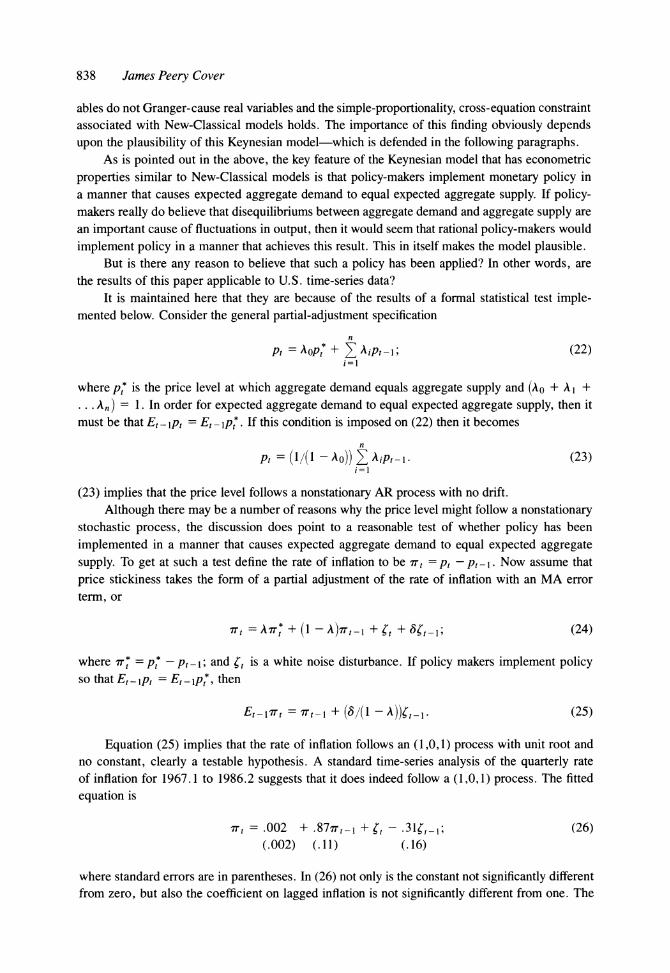
mented below. Consider the general partial-adjustment specification n

Pt = AoPt* + AiPt-1i; (22) i=1

where pt* is the price level at which aggregate demand equals aggregate supply and (Ao + A + ... An) = 1. In order for expected aggregate demand to equal expected aggregate supply, then it must be that Et, -IPt = Et-l p*. If this condition is imposed on (22) then it becomes

n

Pt = (1/(1 -Ao)) A iPt -. (23) i=1

(23) implies that the price level follows a nonstationary AR process with no drift.

Although there may be a number of reasons why the price level might follow a nonstationary stochastic process, the discussion does point to a reasonable test of whether policy has been

implemented in a manner that causes expected aggregate demand to equal expected aggregate supply. To get at such a test define the rate of inflation to be 7Tt = Pt - Pt--. Now assume that

price stickiness takes the form of a partial adjustment of the rate of inflation with an MA error term, or

7Tt = AT* + (1 - A)7rt_1 + +t

-+ •t-1; (24)

where 7ri = p t* - P -1; and rt is a white noise disturbance. If policy makers implement policy so that Et,- Pt = Et,- Pt*, then

E,-17 t = 7T-i + (8/(1 - A)),-1. (25)

Equation (25) implies that the rate of inflation follows an (1,0,1) process with unit root and no constant, clearly a testable hypothesis. A standard time-series analysis of the quarterly rate of inflation for 1967.1 to 1986.2 suggests that it does indeed follow a (1,0,1) process. The fitted equation is

rt, = .002 + .87wr-1 + s,

- .31sr_1;

(26) (.002) (.11) (.16)

where standard errors are in parentheses. In (26) not only is the constant not significantly different from zero, but also the coefficient on lagged inflation is not significantly different from one. The


F-statistic of the joint null hypothesis is only 1.85, hence it is concluded that one cannot reject the

joint hypothesis that during 1967.1-1986.2 the price-level exhibited stickiness of the form (24) and monetary authorities implemented policy in a manner that caused expected aggregate demand to equal expected aggregate supply.7

7. This is the case whether one uses standard tables of the F- and t-distributions, or the empirical tables found in

Dickey and Fuller [5].

References

1. Barro, Robert J., "Unanticipated Money Growth and Unemployment in the United States." American Economic Review, March 1977, 101-15.

2. - , "Unanticipated Money, Output, and the Price Level in the United States." Journal of Political Economy, August 1978, 549-80.

3. - and Herschel I. Grossman, "A General Disequilibrium Model of Income and Employment." American Economic Review, March 1971, 82-93.

4. Clower, Robert W. "The Keynesian Counter-Revolution: A Theoretical Appraisal," in The Theory of Interest Rates, edited by F Hahn and F Brechling. London: McMillan, 1965.

5. Dickey, David A. and Wayne A. Fuller, "Likelihood Ratio Statistics for Autoregressive Time Series with Unit Root." Econometrica, July 1981, 1057-72.

6. Eichenbaum, Martin and Kenneth J. Singleton. "Do Equilibrium Business-Cycle Models Explain Postwar U.S. Business Cycles?" in Macroeconomics Annual: 1986, edited by Stanley Fischer. Cambridge, Mass.: MIT Press, 1986.

7. McCallum, Bennett T., "Rational Expectations and the Natural Rate Hypothesis: Some Consistent Estimates." Econometrica, January 1976, 43-52.

8. , "Price-Level Adjustments and the Rational Expectations Approach to Macroeconomic Stabilization Policy." Journal of Money, Credit, and Banking, November 1978, 418-36.

9. - , "Monetarism, Rational Expectations, Oligopolistic Pricing, and the MPS Econometric Model." Jour- nal of Political Economy, February 1979, 57-73.

10. - , "On the Observational Inequivalence of Classical and Keynesian Models." Journal of Political Econ- omy, April 1979, 395-402.

11. - , "Price-Level Determinacy with an Interest-Rate Policy Rule and Rational Expectations." Journal of Monetary Economics, November 1981, 319-29.

12. Mishkin, Fredric S., "Does Anticipated Policy Matter? An Econometric Investigation." Journal of Political Economy, February 1982, 22-51.

13. - , "Does Anticipated Aggregate Demand Policy Matter? Further Econometric Results." American Eco- nomic Review, September 1982, 788-802.

14. Patinkin, Don. Money, Interest, and Prices, 2nd edition. New York: Harper and Row, 1965. 15. Sargent, Thomas J., "Rational Expectations, the Real Rate of Interest, and the Natural Rate of Unemployment."

Brookings Papers on Economic Activity, 2, 1973, 429-72. 16. - , "A Classical Macroeconometric Model for the United States." Journal of Political Economy, April

1976, 207-37. 17. - , "Causality, Exogeneity, and Natural Rate Models: Reply to C. R. Nelson and B. T. McCallum."

Journal of Political Economy, April 1979, 403-9. 18. - and Neil Wallace, " 'Rational' Expectations, the Optimal Monetary Instrument, and the Optimal Money

Supply Rule." Journal of Political Economy, April 1975, 241-54.

a keynesian macroeconomic model with new-classical ...lrazzolini/gr1988.pdfa keynesian macroeconomic...

Documents