a hyperheuristic approach for dynamic multilevel

Gokce, M., A., Beygo, B., Emekci, T. / Journal of Yasar University, 2017, 12/45, 14-31

A Hyperheuristic Approach for Dynamic Multilevel

Capacitated Lot Sizing with Linked Lot Sizes for APS

implementations

İleri Planlama ve Çizelgeleme (APS) Uygulamaları için Kapasiteli Çok Seviyeli

Dinamik Lot Belirleme Problemine Hiper-Sezgisel Yaklaşım

Mahmut Ali GOKCE, İzmir University of Economics, [email protected]

Berkay BEYGO, [email protected]

Turgut EMEKCI, [email protected]

Abstract: This study is concerned with solving real-life sized APS (Advanced Planning and Scheduling) problems

practically. Specifically, the problem of Multilevel Capacitated Lot Sizing Problem with linked lot sizes (MLCLSP-L) is

considered. The problem is a classical, practical and notoriously hard problem. We propose a new modeling technique

for MLCLSP-L based on a GA-driven hyperheuristic, which enables modeling of some issues previously not modeled.

Proposed model uses an indirect representation by allowing GA search through a space of low level heuristics’

combinations. Each one of the low level heuristics is simple and determines the detailed production plan of a machine

in a period. The solution is constructed through combination of these low level heuristics. New model is demonstrated

by solving moderate size test problem along with software developed.”

Keywords: APS implementation, multilevel capacitated lot sizing problem with linked lot sizes; hyperheuristic; genetic algorithm; production

planning; constructive heuristics

Öz: Bu makale gerçek yaşam boyutlarındaki İleri Planlama ve Çizelgeleme (İPÇ)problemlerinin çözümü

üzerinedir.Özellikle, kapasite kısıtı altında çok seviyeli lot boyutlandırma ve çizelgeleme problemi çalışılmıştır. Bu

problem, pratik değeri yüksek ve akademik olarak da son derece zor bir problemdir. Problemin çözümü için Genetik

Algoritmalara (GA) dayalı bir hiper-sezgisel yöntem önerilmektedir. Önerilen yöntem daha önce kullanılan

yöntemlerleeile modellenmemiş bazı durumların modellenmesine de olanak tanır.Önerilen model, doğrudan olmayan

bir temsil kullanarak, GA’nın düşük seviyeli sezgisellerin kombinasyonlarından oluşan uzayında gezinerek çözüm

aramasına dayanır. Her düşük seviyeli sezgisel aslında, bir makineye, bir zaman periyodunda yükleme yapan basit

algoritmadır.Esas çözüm, farklı düşük seviyeli sezgisellerin makinalarda, periyotlar boyunca kombinasyonu ile

oluşturulur.Bu yeni model gerçek yaşam boyutunda bir problemin çözümünde, geliştirilen yazılım ile beraber

kullanılmıştır.

Anahtar Kelimeler: İleri Planlama ve Çizelgeleme (İPÇ=APS) uygulaması, Çok seviyeli lot boyutlama ve çizelgeleme, hiper

sezgisel, genetic algoritma, üretim planlama, yapısal sezgisel

1. Introduction First, we introduce Advanced Planning and Scheduling Systems and their importance. Then, multilevel lot sizing and

scheduling problem is described in detail and its relationship to APS systems is established.

1.1. Advanced Planning and Scheduling Systems The computerized production planning and control systems were developed gradually over the last thirty years, starting

with Material Requirements Planning (MRP), and followed by Manufacturing Resources Planning (MRP-II), Enterprise

Resource Planning (ERP) and finally Advanced Planning and Scheduling (APS) (Steger Jensen et al. 2011).

Since early 1990s, APS started to appear on the integrated systems’ market. APS is formally defined as

“Techniques that deal with analysis and planning or logistics and manufacturing during short, intermediate and long-

term time periods. APS system describes any computer program that uses advanced mathematical algorithms and/or

logic to perform optimization or simulation on finite capacity scheduling, sourcing, capital planning, resource planning,

forecasting, demand management, and others. These techniques simultaneously consider a range of constraints and

business rules to provide real-time planning and scheduling, decision support, available-to-promise, and capable-to-

promise capabilities. APS often generates and evaluates multiple scenarios.” (Blackstone and Cocks in APICS

dictionary, 2005)


15

APS systems are generally used in conjunction with ERP systems, either as add-ons or direct integral components

of ERP systems, creating the support mechanism for planning and decision-making (Kreipl and Dickersbach, 2008).

Figure 1 shows the conceptual framework of Advanced Planning and the Supply Chain Planning (SCP)matrix

(Fleischmann et al. 2008), the multi level lot sizing and scheduling problem discussed in this paper, cover the planning

tasks of lot-sizing and machine scheduling. Additionally, they are linked to short term sales planning as a capable-to-

promise logic (Kilger and Schneewiss, 2005).

Figure 1. Supply Chain Planning (SCP) Matrix (Fleischmann et al., 2008, p.87)

The great promise APS systems has been that, when implemented correctly, an APS system allows companies, use

already available capacity much more efficiently, and therefore contributing more to the bottomline. This has led to a

vast amount of literature on APS development.

Stadler (2005 ) discusses issues and challenges of today’s APS will in three main categories. The first of those

categories are module improvement where most importantly Production planning and detailed scheduling of APS is

discussed. Lot sizing and scheduling is the main technical problem to be solved for this purpose and therefore stands as

the most important technical barrier to a more successful APS implementation

The exceeding majority of the publications use MILP (Mixed Integer Linear Programming) for modeling and

solving these problems. Studies suggest that there are difficulties with implementing and using APS systems (Zoryk-

Schalla et al., 2004, Lin et al., 2007) and many companies report on “failed” implementations and that expected benefits

have not been achieved (De Kok and Graves, 2003; Günter, 2005)

One of the main reasons of these failures is the promised benefits of being able to perform dynamic lot sizing and

machine scheduling together. Unfortunately, the natural limitations of MILP modeling kick in for realistic size

problems and users are either left with unsolvable problems and/or overly simplified versions of their problems leading

to frustrations. Therefore there is a great need for models capable to handle real life size APS (lot sizing and scheduling)

problems practically.

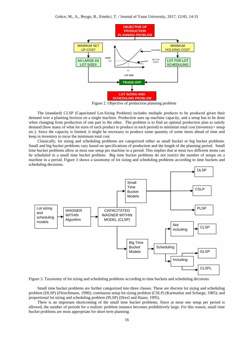
1.2. The Dynamic Multi-LevelLot Sizing and SchedulingProblem In many production environments, machines (or other resources) have to go through some sort of setup before

production can begin. So ideally, one would try to produce as large batches of any product as possible, once the

machine is setup. This causes holding cost and the necessity of striking a balance between setup and holding costs,

giving birth to lot sizing problems (Figure 2).


16

Figure 2. Objective of production planning problem

The (standard) CLSP (Capacitated Lot-Sizing Problem) includes multiple products to be produced given their

demand over a planning horizon on a single machine. Production uses up machine capacity, and a setup has to be done

when changing from production of one part to the other. The problem is to find an optimal production plan to satisfy

demand (how many of what lot sizes of each product to produce in each period) to minimize total cost (inventory+ setup

etc.). Since the capacity is limited, it might be necessary to produce some quantity of some items ahead of time and

keep in inventory to incur the minimum total cost.

Classically, lot sizing and scheduling problems are categorized either as small bucket or big bucket problems.

Small and big bucket problems vary based on specifications of production and the length of the planning period. Small

time bucket problems allow at most one setup per machine in a period. This implies that at most two different items can

be scheduled in a small time bucket problem. Big time bucket problems do not restrict the number of setups on a

machine in a period. Figure 3 shows a taxonomy of lot sizing and scheduling problems according to time buckets and

scheduling decisions.

Figure 3. Taxonomy of lot sizing and scheduling problems according to time buckets and scheduling decisions

Small time bucket problems are further categorized into three classes. These are discrete lot sizing and scheduling

problem (DLSP) (Fleischmann, 1990); continuous setup lot sizing problem (CSLP) (Karmarkar and Scharge, 1985); and

proportional lot sizing and scheduling problem (PLSP) (Drexl and Haase, 1995).

There is an important shortcoming of the small time bucket problems. Since at most one setup per period is

allowed, the number of periods for a realistic problem instance becomes prohibitively large. For this reason, small time

bucket problems are most appropriate for short term planning.

Lot sizing

and

scheduling

models

Small

Time

Bucket

Models

Big Time

Bucket

Models

DLSP

CSLP

PLSP

CLSP

CLSPL

WAGNER

WITHIN

Algorithm

GLSP

CAPACITATED

WAGNER WITHIN

MODEL (CLSP)

Scheduling

Including

Not

including

MINIMUM

HOLDING COST

OBJECTIVE OF

PRODUCTION

PLANNING PROBLEM

AS LARGE AS

LOT SIZES

LOT FOR LOT

SCHEDULING

TRADE-OFF

LOT SIZING AND

SCHEDULING PROBLEM

LOT SIZE

COST SET UP

COST

HOLDING

COST

Q*

TC*

MINIMUM SET

UP COST


17

The capacitated lot sizing problem is the basis of big time bucket lot sizing problems. Different from small time

bucket problems, it is possible to make more than one setup on a machine in a period in big bucket models. This enables

modeling longer term planning problems. Unfortunately, the problems get also very hard to solve. Multilevel

capacitated lot sizing is the most realistic but probably hardest of big time bucket problems. In multilevel capacitated lot

sizing problem (MLCLSP), planning is not only done for a final product, but also for the components and subassemblies

that make up an end product, given its bill of material (BOM, Figure 4). Production at one level leads to demand for

components at lower levels (dependent demand). The end product’s demand is usually supplied by a master production

schedule (MPS), which in turn is shaped by market demand. For the MLCLSP solution to be converted to a feasible

production schedule, a minimum planned lead-time of one period must be introduced for each component product.

Figure 4. Bill of Material (Gozinto structure) for MLCLSP

An overview of lot sizing and scheduling problems (focusing more on small time buckets) can be found in Drexl

and Kimms (1997). Meyr (1999) reviews small bucket problems with sequencing decisions.

Denizel and Süral (2006) provide various MIP formulations. Karimi et al. (2003) provides a review of capacitated

lot sizing models. A more recent review by Quadt and Kuhn (2008) provide standard MIP formulations of CLSP and its

extensions. Specifically, they provide extensions of standard MIP CLSP models based on back-orders, setup carry-

over, sequencing, and parallel machines. These various extensions of CLSP result in more practical, but harder

problems. Most important extensions are inclusion of parallel machines (at least one), setup carryover, backlogging and

sequencing.

The existence of parallel machines implies that there is no unambiguous part-machine assignment. Each part, then,

can be produced on more than one machine, possibly with different unit production and setup times.

The inclusion of setup carry-over (also referred to as linked lot sizes) mean that the machine can carry its setup

state from the end of period to the start of the next period. This means last part produced on a machine in a period, can

continue its production without an additional setup in the immediately following period on the same machine. Therefore

a CLSP with linked lot sizes must determine the last (and first) parts on every machine for each period.

As a final extension, scheduling decisions for all parts can be included into the problem. In this case, a total

sequence of parts on a machine in a period must be determined. This extension is useful in modeling when sequence-

dependent setups exist. Examples for this case can be paint shops, fabric dying and chemical industry. If the setups are

not sequence-dependent, this extension will add unnecessary complexity to the problem.

In many real-life problems where the utilizations are high, it is especially important to include backlogging and

linked lot sizes.

The problem basically relates to the production planning process. In most real-world situations, decision-makers

face multilevel gozinto structures (BOM) and therefore need solution procedures capable of dealing with these.

In this paper, we present a new modeling approach to dynamic multilevel capacitated lot sizing problem with

linked lot sizes (MLCLSP-L) for general product structures based on a GA-driven hyperheuristics. MLCLSP-L is a

practically important and theoretically challenging problem.

MLCLSP-L is one of the hardest and most practical of the lot sizing and scheduling problems to solve. There are

mainly Mixed Integer Programming (MIP) approaches and relaxations of MIP formulations as well as direct

applications of meta-heuristics to this problem.

Bitran and Yanasse (1982) and Florian et al. (1980) have shown that even single item capacitated lot sizing

problem (CLSP) is NP-hard. Even the feasibility problem (”Does a solution exist?”) is already NP-complete for the

single-level problem if there are setup times. Chen and Thizy (1990) have proved that multi-item capacitated lot sizing

problem (MCLSP) with setup times is strongly NP-Hard. Since MCLSP is a special case of the problem considered in

this study (where every item has only single level), MLCLSPL is at least strongly NP-hard. For this reason, exact

methods and commercial software packages for obtaining optimal solutions are not very helpful when the problem

instances get large.

Based on these results, it is unlikely that we can develop any effective optimal algorithm for this problem.

Therefore, research on developing effective heuristics has been a profitable research area for a long time.


18

2. Literature Review There is a vast amount of literature on lot sizing and scheduling problems. For practical purposes, this section gives a

limited review of some of the models used to solve MLCLSP-L. Also some background in hyperheuristics, especially

relating to use of metaheuristics (GA)s and scheduling–planning problems is provided.

Literature on solving MLCLSP-L is composed of papers using one of the following two groups of methods.

First group includes papers based on mathematical programming and LP or Lagragean relaxations of MIP models.

Tempelmeier and Derstroff (1996) provide one of the earlier examples of a heuristic based on lagrangean

relaxations of MIP models. One of the last examples of MIP based approaches comes from Tempelmeier and Buschkühl

(2009). They provide a lagrangean heuristic for solving MLCLSP-L. The authors demonstrate his model with two

different data sets. First set is a generated data set composed if 3-6 resources for 10, 20 or 40 parts over a planning

horizon of 4,8 or 16 periods. They also demonstrate their method with an industrial data set of 77 items with one level

deep BOM.

Tempelmeier (2003) and Suerie and Stadtler (2003) uses plant location analogy to get tighter bounds for their

MIP formulations.

Stadtler (1996), Meyr (1999), Staggemeier and Clark (2001), Suerie (2005), Pochet and Wolsey (2006) provide

excellent reviews of such models.

The second group includes papers based on meta-heuristics. When utilizing a meta-heuristic for modeling

MLCLSP-L, the important decisions are which meta-heuristic to use, solution representation, evaluation,

neighbourhood and/or operators to be used. Simulated annealing (SA), tabu search (TS) and genetic algorithms have

been applied. Jans and Degraeve (2007) provides an excellent review on meta-heuristic approaches to dynamic lot

sizing problems.

A great majority of the literature on MLCLSP-L mentioned above tries to minimize setup cost as well. For this a

setup cost is assumed to be given. But in reality setup consideration is mostly based on time not cost. Also this assumes,

based on setup unit time cost, a presumed weight compared to production and inventory costs. We assume a setup time,

rather than a setup cost. In this setting setup consumes from available machine capacity.

The main goal of hyper-heuristics is to get rid of the need of having the heuristic have information on the problem

and to enhance the generality at which meta-heuristics and optimization systems can operate, all the while providing

good quality solutions quickly (Burket et al., 2003). Hyperheuristics are defined simply as “heuristics which choose

heuristics ” (Burket et al., 2003). Although history of the idea of using heuristics to choose heuristics goes way back,

hyperheuristic name has first been used by Cowling et al. (2001).

Especially during the last five years, more and more research papers on hyperheuristics are published.

Hyperheuristic based methods have been published for solving different scheduling problems (nurse, trainer,

timetabling etc.), But except Bai et al. (2008) on fresh produce inventory control and shelf allocation and Tay and Ho

(2008) on job shop scheduling, there are not many applications of hyperheuristic based methods for production related

problems. Ochoa (2009) presents an extensive list of book chapters, conference proceedings and journal papers on

hyperheuristics and related approaches. Ozcan et al. (2008) provides an in-depth anaylsis of hyperheuristics. An

excellent review of recent developments on hyperheuristics is given by Chaklevitch and Cowling (2008).

Exact methods for MLCLSP-L suffer from the fact that solving any realistic size problem takes too long. Other

heuristic based methods so far (direct applications of metaheuristics etc.) were of the kind that mostly had parameter

dependent performance and required considerable parameter optimization. Different problems are faced everyday, with

different characteristics. So a solution to MLCLSP-L must be robust enough to handle these differences and hopefully

produce “acceptable quality” results.

For any solution for MLCLSP-L method to make a practical impact in industry, it should be able to solve instances

with 100 or more parts which are stil not achieved. (Staedler, 2003)

To the best of our knowledge, there is no other hyperheuristic based models published for solving MLCLSP-L yet.

The proposed new modeling is more independent of problem structure than previous models. It also allows for

modeling issues, previously not possible (like time heterogeneous data)

MLCLSP-L is a new challenging area for hyperheuristics. The authors believe there is great potential for use of

hyperheuristics in general production related problems, especially for the industrial sizes.

In the remainder of this paper, the proposed hyperheuristic approach to MLCLSP is presented in the next section.

Section 3 demonstrates the proposed model by solving a test problem and presenting results from a large experimental

design. Lastly, section 4 summarizes conclusions and gives directions for future work.

3. Proposed Model We propose a genetic algorithm (GA) driven constructive hyperheuristic method to solve MLCLSP-L. Our approach

dictates a genetic algorithm managing a number of low level heuristics. Each low level heuristic myopically tries to find

the production numbers and partial sequence of jobs on a machine in a period (the first and last parts to be produced)

based on simple objectives. Therefore each low level heuristic is responsible for only determining production plan of a


19

machine in a period. Each low level heuristic constructs part of the solution, but collection of these heuristics for all

machines give a complete solution.

Due their simplicity, as easy to calculate as they are, these low level heuristics with simple objectives, do not

consider the whole picture. Therefore, one would expect that if one such heuristic is applied to solve the whole problem,

for all machines and for all the periods, one would attain a possibly poor, suboptimal solution. Individual low level

heuristics may be especially effective at certain stages of constructing the solution while performing poorly at some

latter stage. For this reason, we hope several low level heuristics combined properly may produce better solutions.

Our approach is based on the fact that an optimal solution for MLCLSP-L is a solution which balances shortage

vs. inventory costs without violating capacity constraints. Low level heuristics are single objective, without considering

remifications on other measures relating to the overall performance of the plan, but proper permutation of such low

level heuristics might give robust good solutions in reasonable time. The hyperheuristic is responsible for searching

through these combinations of low level heuristics, without any information relating to problem domain (Figure 5).

Figure 5. Heuristic vs. Solution Space

In this setting, the genetic algorithm utilizes an indirect representation of the problem. For GA, a solution is

therefore just a combination of low level heuristics. Any solution in the hyper-heuristic space then has to be translated

into a real solution by a deterministic simulation of low level heuristics.

3.1. Genetic Algorithm Driven Hyperheuristic Details A genetic algorithm (GA) is a search technique used in computing to find exact or approximate solutions to

optimization and search problems. It is implemented as a computer simulation of population of chromosomes

(individuals) representing solutions to the problem. This population evolves through generations following a cycle of

selection, crossover, mutation, toward better solutions and converging to a good solution. Genetic algorithms are a

particular class of evolutionary algorithms that use techniques inspired by evolutionary biology such as inheritance,

mutation, selection, and crossover. Any genetic algorithm can be determined exactly by determining the following:

Representation: GA driven hyperheuristics uses a matrix notation. A M x T matrix represents a

solution, where M is the number of machines available and T is the planning horizon. Cell (m,t) contains the

low level heuristic to be used to find production plan of machine m in period t (Figure 6).

T

=1

T

=2

. . T

=m

Machine 1 H1 H2 . . H9

Machine 2 H5 . . . H5

.

. . . .

.

.

. . . .

.

Machine M H4 . . . H3

Figure 6. Chromosome Representation

Initialization: Each individual in the population is initialized by randomly assigning heuristics from

the low level heuristics set (i.e. each cell in the encoded solution is assigned a low level heuristic from the list

of low level heuristics with equal probability using a random number generator). As an option, the user has the

possibility to generate 10 times many individuals compared to the population size and keep the best population

size to get a better starting solution.

Selection: Selection mechanism determines how individuals are picked from the population for

crossover and for forming the next generation’s population after crossover and mutation.

Not one-to-one and covering

Solution

Space

Hyperheuristic

Space


20

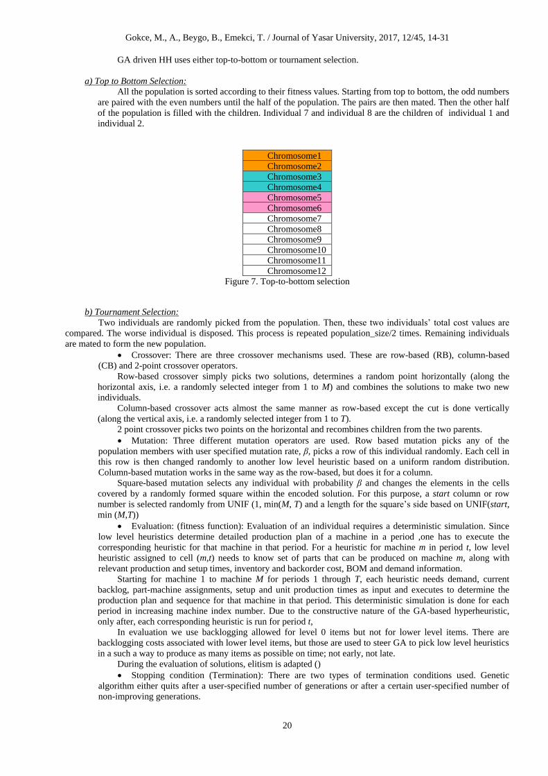
GA driven HH uses either top-to-bottom or tournament selection.

a) Top to Bottom Selection:

All the population is sorted according to their fitness values. Starting from top to bottom, the odd numbers

are paired with the even numbers until the half of the population. The pairs are then mated. Then the other half

of the population is filled with the children. Individual 7 and individual 8 are the children of individual 1 and

individual 2.

Chromosome1 Chromosome2 Chromosome3 Chromosome4 Chromosome5 Chromosome6

Chromosome7 Chromosome8 Chromosome9 Chromosome10 Chromosome11

Chromosome12 Figure 7. Top-to-bottom selection

b) Tournament Selection:

Two individuals are randomly picked from the population. Then, these two individuals’ total cost values are

compared. The worse individual is disposed. This process is repeated population_size/2 times. Remaining individuals

are mated to form the new population.

Crossover: There are three crossover mechanisms used. These are row-based (RB), column-based

(CB) and 2-point crossover operators.

Row-based crossover simply picks two solutions, determines a random point horizontally (along the

horizontal axis, i.e. a randomly selected integer from 1 to M) and combines the solutions to make two new

individuals.

Column-based crossover acts almost the same manner as row-based except the cut is done vertically

(along the vertical axis, i.e. a randomly selected integer from 1 to T).

2 point crossover picks two points on the horizontal and recombines children from the two parents.

Mutation: Three different mutation operators are used. Row based mutation picks any of the

population members with user specified mutation rate, β, picks a row of this individual randomly. Each cell in

this row is then changed randomly to another low level heuristic based on a uniform random distribution.

Column-based mutation works in the same way as the row-based, but does it for a column.

Square-based mutation selects any individual with probability β and changes the elements in the cells

covered by a randomly formed square within the encoded solution. For this purpose, a start column or row

number is selected randomly from UNIF (1, min(M, T) and a length for the square’s side based on UNIF(start,

min (M,T))

Evaluation: (fitness function): Evaluation of an individual requires a deterministic simulation. Since

low level heuristics determine detailed production plan of a machine in a period ,one has to execute the

corresponding heuristic for that machine in that period. For a heuristic for machine m in period t, low level

heuristic assigned to cell (m,t) needs to know set of parts that can be produced on machine m, along with

relevant production and setup times, inventory and backorder cost, BOM and demand information.

Starting for machine 1 to machine M for periods 1 through T, each heuristic needs demand, current

backlog, part-machine assignments, setup and unit production times as input and executes to determine the

production plan and sequence for that machine in that period. This deterministic simulation is done for each

period in increasing machine index number. Due to the constructive nature of the GA-based hyperheuristic,

only after, each corresponding heuristic is run for period t,

In evaluation we use backlogging allowed for level 0 items but not for lower level items. There are

backlogging costs associated with lower level items, but those are used to steer GA to pick low level heuristics

in a such a way to produce as many items as possible on time; not early, not late.

During the evaluation of solutions, elitism is adapted ()

Stopping condition (Termination): There are two types of termination conditions used. Genetic

algorithm either quits after a user-specified number of generations or after a certain user-specified number of

non-improving generations.


21

A total of ten (10) low level heuristics are used for the propose solution. The details of these low level heuristics

are given in the next section.

3.2. Low level Heuristics The following notation is used to explain the low level heuristics.

t = Current period

m = Current machine

Pt,m = Set of parts that can be produced on on machine m in period t

Di,t = (Remaining) Demand of part i in period t

Bi,t = (Remainig) Backlog amount of part i at the beginning of period t.

CBit = Cost matrix according to backlog for item i in period t

CDi,t = Cost matrix according to (potential backlogging) demand for item i in period t

Cm t = (Remaining) capacity of machine m in period t

si,m = Setup of item i on machine m

pi,m = Unit production of item i on machine m

Heuristic 1 (H1) – Minimize Backlogging Cost

H1 tries to minimize backlogging costs. It first tries to produce the backlogged items in Pt,m in decreasing

baclogging cost (CBi,t) amount. If the machine still has enough capacity, the heuristic tries to produce the demands in

period t in decreasing potential backlogging cost (CDi,t, demand not satisifed for t becomes backlog). If the machine still

has enough capacity, it tries to produce items with demand in t+1 in decreasing CDi,t+1 amount and stops.

CBi,t = Min tgingbackUnit

qtygingBack

capacitytodueqtyprodMax

tesprerequisitodueqtyprodMax

cos_log_*

_log

,_____

,_____

CDi,t = Min tgingbackUnit

qtyDemand

capacitytodueqtyprodMax

tesprerequisitodueqtyprodMax

cos_log_*

_

,_____

,_____

Heuristic 2 (H2) – Minimizing Set-up Time

H2 tries to minimize the set-up cost. If there is a setup on the machine, the machine first tries to produce the

backlog and all the remaining demand until the end of the planning horizon of this item. If there is still capacity left, H2

finds the item with highest number of backlogs, performs setup for this part and stops. If there are no items with

backlog, finds highest demand in Pt,m, performs setup and stops. If no item with demand in Pt,m in period t, check t+1

and stop.

Heuristic 3 (H3) – BOM_Weight

H3 first calculates BOM weight of parts in Pt,m with positive backlog. Schedule backlogs in decreasing BOM

weight. If there is stil capacity left after all items with backlogs scheduled, repeat with parts that have demand in t. If

still there is capacity left, repeat for t+1. Stop.

Weight of a part is the number of that part that is required for one level 0 item.

BOM_Weight of Part i: Weight of i + (Weight of all parts i i directly goes into)

If a part is in more than one BOM, final BOM_Weight is a average of BOM_Weights from different BOMs

weighted on demand of the corresponding endi tem.

Heuristic 4 (H4) - BOM_Depth

H5 first schedules backlogged items in lower levels of the BOM. Any ties based on the BOM level is broken by

scheduling smaller part numbers first. If capacity left, it schedules items with demand in period t in the same manner. If

still there is capacity left, H5 goes through list of items in Pt,m with demand in period t+1 and stops.

Heuristic 5 (H5) - Min. Potential Backlog

H5 is a modification of H1. Instead of first going through the list of backlogged items and then items with demand

in Pt,m, it schedules items in decreasing potential backloggin cost ( (backlog+this period’s demand)*unit

backlogging cost). If all backlog and period t demand is scheduled and there is capacity left, tries to schedule items with

demand in t+1 in decreasing CDi,t+1.

Heuristic 6 (H6) - Quickest BOM_Depth

H6 is a modification of H4. Different from H4, H6 breaks ties between items that have same BOM depth level in

favor of item with shorter processing time on machine m.


22

Heuristic 7 (H7) - Minimum Unit Production Time First

H7 first schedules on machine m, parts that can be produced fastest on machine m. First backlogs of these items

are scheduled. If capacity remains, demand of these items are scheduled.

Heuristic 8 (H8) – Dynamic BOM_Weight

H8 is a modification of H3. Each step BOM weight of parts are updated as they are produced in the following

way:

BOM Weight of part i = BOM Weight of part i * [1-(total number of part i produced so far/Planning horizon total

demand of part i ) ]

Heuristic9 (H9) – Min. Inventory – Modified Holding Cost

H9 is a modification of H5. H9 takes the parts in Pt,m and schedules them in decreasing cost value. The cost for

part i in Pt,m is calculated as:

Max. Number that can be produced of i * modifiedInvCost of i

modifiedInvCost of i = inventory cost of i - (inventory costs of all items that directly go into this item)

Heuristic 10 (H10) Resolve Capacity

H10 aims remedy possible capacity problems by pulling demand from next period to this period. H10 checks if

possible capacity problems exist in period t+1. (This is done by finding out total setup plus production time of all items

that have deman in t+1 if they were to be produced in the fastest possible machine based on machine-part matrix. If

capacity of any machine in t+1 goes below zero, capacity problems exist )

For the machines capacity problems exist, H10 tries to move enough demand to machines with excess capacity

this semester in decreasing BOM level, until capacity problem is remedied. This does not mean H10 is a repair function.

But under certain conditions (existence of a possible capacity problem following period), H10 favors earlier production.

If capacity problem does not exist in t+1, check t+2, and try to remedy capacity problem, then stop.

Since setup carry-over is allowed, the proposed model must be able to give the starting and ending jobs for each

machine in each period. Each low level heuristic first determines the lot sizes for the machine and period it is executed

for. Then every low level heuristic checks if there is already a setup on the machine and if there is a lot formed for that

part. If there is the part for which the machine is already scheduled for, that part is scheduled first in that period,

removing one setup. If there is no lot formed for the part the machine is already setup for, but there is a part scheduled

on the same machine in previous period (not the first part) for which a lot is formed also this period. These lots are

made the last and first of previous and this period, to save from the setup.

The proposed model is coded in C# with a user interface that allows easily uploading data for a different instance

from a text or .csv file. The proposed model is capable of solving any general product structure.

The user interface also allows the user to see the progress of the solution, number of evaluations, current solution

and details of the final solution. The detailed plan can be saved in .csv format for future use or comparisons. A

screenshot along with explanations of the software is appendix 1

4. Computational Study We present the proposed method to solve MLCLSP-L with an extended computational study on a sample problem.

The problem chosen is taken from Ozturk (2007) or Öztürk and Örnek (2009). This specific example is chosen because

it is a small-moderate size problem for which the mathematical model is developed and published and results are freely

accessible. The run-time to solve the mathematical model is reported to be 1800 seconds on a system with Intel Core 2

Duo 2.66 GHz CPU with 2 GB of RAM running Windows XP Professional system. The sample problem has a planning

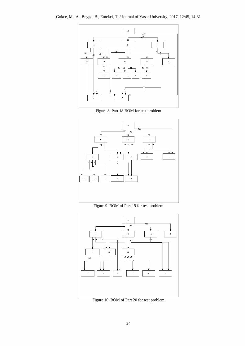
horizon (T) of 10 periods with 20 parts. There are three end items (level 0) with 3 and 4 levels of BOM depth. There are

12 machines on which the production takes place. The gozinto matrix is given in table 1. Figures 8 through 10 show the

BOM of level 0 items. Part setup and unit production times are given in tables 2 and 3. The machine capacities are

given in table 4. The test problem has demand of 89 for part 20, 179 for part 19 and 352 for part 18. The demand for

lower level items are calculated through BOM explosion calculus.

We use the ten low level heuristics presented in section 2.2.

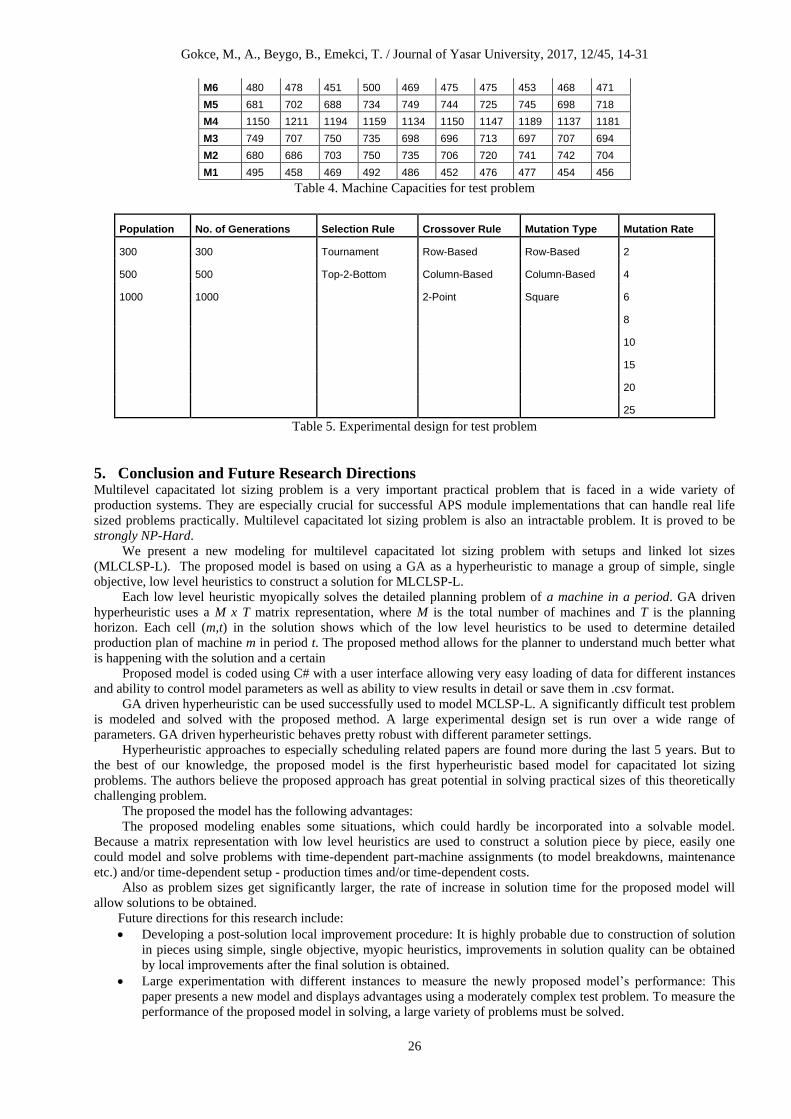
The test problem is solved with a large experimental design for parameters of GA. One of the critiques on using

metaheuristics is that even when used as a hyperheuristic, significant amount of effort has to be spent parameter tuning.

We would like to see if this is the case here.

The experimental design is presented in table 5. This design corresponds to a total of 3x3x2x3x3x8 = 1296

combinations of parameters. Each combination of the experimental design is run with 5 different random seeds and

averaged over. Therefore the test problem is solved a total of 6480 times.

The best solution obtained by the hyperheuristic is within 96,9% of the optimal but in just 129.85 seconds a result at

96,2% of the optimal value can be obtained (pop_size= 500, gen=300, row-based mutation with 0.15 probability,

column-based crossover and top-to-bottom selection). The best parameter setting is found out to be where the

population size is 500, a row-based mutation is applied with a probability of 0.15, column-based crossover and pairing

from top-to-bottom selection is applied for 200 generations. When larger problems are solved, the increase in the


23

computational time of the hyperheuristic will much less compared to the increase in time required for the mathematical

model.

When the problem size is doubled to 20 periods (by repeating demands for periods 1-10 for periods 11-20), it only takes

hyperheuristic method 158 seconds (additional 28 seconds) to find a solution with a cost of 64012 and optimal solution

from the mathematical model is stopped within 3600 seconds without finding the optimal solution.

The proposed model achieves a best solution of 96.94% of optimality. Overall average solution quality is 93.1% with a

standard deviation of 1.27% for the experimental design in table 5.

The large experimentation with the parameters show almost a perfect normal distribution around the mean. 68.7% of the

solutions are within +/- 1σ, 94.4% are within +/- 2σ and +/- 3σ covers the whole range.

1 2 3 4 5 6 7 8 9 10 11 12 13 14 15 16 17 18 19 20

BOM P20 P19 P18 P17 P16 P15 P14 P13 P12 P11 P10 P9 P8 P7 P6 P5 P4 P3 P2 P1

P20

P19 0

P18 0 0

P17 2 0 0

P16 1 2 0 0

P15 0 1 1 0 0

P14 0 0 2 0 0 0

P13 0 0 10 4 0 0 0

P12 0 0 0 3 1 2 0 0

P11 0 0 0 0 1 0 1 0 0

P10 4 0 0 0 0 2 1 0 0 0

P9 0 3 0 0 0 0 1 0 0 0 0

P8 0 0 0 0 0 0 0 4 0 0 0 0

P7 0 0 15 0 0 0 5 1 1 0 0 0 0

P6 0 0 0 12 0 0 0 0 0 2 0 0 0 0

P5 0 0 0 0 0 0 0 0 0 3 0 0 0 0 0

P4 0 0 0 0 0 0 0 0 0 2 0 0 0 0 0 0

P3 0 0 0 0 6 0 0 0 0 0 4 0 0 0 0 0 0

P2 16 0 0 0 0 8 0 0 0 0 0 2 0 0 0 0 0 0

P1 0 11 0 0 0 0 0 0 0 0 0 4 0 0 0 0 0 0 0

Lead Time 1 1 1 2 1 1 1 1 2 1 1 2 1 1 1 1 1 1 3 1

Lot Size 15 10 5 30 30 20 10 60 100 60 30 20 240 120 200 150 100 120 100 100

Backorder

C. 12,8 12,4 16,8 4,0 3,2 4,4 5,4 1,4 0,6 1,8 1,2 1,6 0,2 0,2 0,2 0,2 0,2 0,2 0,2 0,2

Holding

Cost 6,4 6,2 8,4 2,0 1,6 2,2 2,7 0,7 0,3 0,9 0,6 0,8 0,1 0,1 0,1 0,1 0,1 0,1 0,1 0,1

Starting

Inv. 0 0 0 0 0 0 0 0 0 0 0 0 0 0 0 0 0 0 0 0

Minimum

SKU 1 1 1 1 1 1 1 1 1 1 1 1 1 1 1 1 1 1 1 1

Starting

Back. 0 0 0 0 0 0 0 0 0 0 0 0 0 0 0 0 0 0 0 0

Table 1. Gozinto Matrix of Test Problem


24

Figure 8. Part 18 BOM for test problem

Figure 9. BOM of Part 19 for test problem

Figure 10. BOM of Part 20 for test problem


25

Pim M12 M11 M10 M9 M8 M7 M6 M5 M4 M3 M2 M1

M20 0,25 1,50 0,00 0,00 0,00 0,00 0,00 0,00 0,00 0,00 0,00 0,00

M19 0,75 0,50 0,00 0,00 0,00 0,00 0,24 0,00 0,00 0,00 0,00 0,00

M18 1,50 1,00 0,00 0,00 0,00 0,00 0,00 0,00 0,00 0,00 0,00 0,00

M17 0,58 0,00 0,00 0,40 0,20 0,00 0,00 0,00 0,00 0,00 0,00 0,00

M16 0,00 0,00 0,10 0,30 0,60 0,00 0,00 0,00 0,00 0,00 0,00 0,00

M15 0,00 0,00 0,25 0,50 0,00 0,00 0,00 0,00 0,00 0,00 0,00 0,00

M14 0,00 0,00 0,75 0,00 0,50 0,00 0,39 0,00 0,00 0,00 0,00 0,00

M13 0,00 0,00 0,00 0,00 0,00 0,50 0,50 0,00 0,00 0,00 0,00 0,00

M12 0,00 0,00 0,00 0,11 0,00 0,20 0,10 0,00 0,00 0,00 0,00 0,00

M11 0,00 0,00 0,00 0,00 0,00 0,30 0,25 0,00 0,00 0,00 0,00 0,00

M10 0,00 0,00 0,00 0,00 0,00 0,00 0,15 0,00 0,00 0,00 0,00 0,00

M9 1,95 0,00 0,00 0,00 0,00 0,20 0,30 0,00 0,00 0,00 0,00 0,00

M8 0,00 0,00 0,60 0,00 0,00 0,00 0,00 0,00 0,30 0,00 0,10 0,00

M7 0,47 0,00 0,00 0,00 0,00 0,34 0,00 0,30 0,00 0,00 0,00 0,10

M6 0,00 0,00 0,00 0,00 0,00 0,00 0,00 0,00 0,00 0,40 0,00 0,00

M5 0,00 0,49 0,00 0,78 0,00 0,00 0,00 0,00 0,60 0,00 0,30 0,00

M4 0,00 0,00 0,00 0,00 0,00 0,00 0,00 0,00 0,00 0,00 0,20 0,20

M3 0,00 0,00 0,00 0,00 0,00 0,00 0,82 0,00 0,10 0,10 0,00 0,00

M2 0,00 0,00 0,00 0,00 0,76 0,00 0,00 0,40 0,00 0,00 0,60 0,00

M1 0,00 0,00 0,00 0,00 0,00 0,00 0,00 0,00 0,30 0,00 0,00 0,25

CAP 250 250 250 250 250 500 500 750 1250 750 750 500

Table 2. Unit production times for test problem

Sim M12 M11 M10 M9 M8 M7 M6 M5 M4 M3 M2 M1

P20 2,50 15,00 0,00 0,00 0,00 0,00 0,00 0,00 0,00 0,00 0,00 0,00

P19 7,50 5,00 0,00 0,00 0,00 0,00 2,40 0,00 0,00 0,00 0,00 0,00

P18 15,00 10,00 0,00 0,00 0,00 0,00 0,00 0,00 0,00 0,00 0,00 0,00

P17 5,80 0,00 0,00 4,00 2,00 0,00 0,00 0,00 0,00 0,00 0,00 0,00

P16 0,00 0,00 1,00 3,00 6,00 0,00 0,00 0,00 0,00 0,00 0,00 0,00

P15 0,00 0,00 2,50 5,00 0,00 0,00 0,00 0,00 0,00 0,00 0,00 0,00

P14 0,00 0,00 7,50 0,00 5,00 0,00 3,90 0,00 0,00 0,00 0,00 0,00

P13 0,00 0,00 0,00 0,00 0,00 5,00 5,00 0,00 0,00 0,00 0,00 0,00

P12 0,00 0,00 0,00 1,10 0,00 2,00 1,00 0,00 0,00 0,00 0,00 0,00

P11 0,00 0,00 0,00 0,00 0,00 3,00 2,50 0,00 0,00 0,00 0,00 0,00

P10 0,00 0,00 0,00 0,00 0,00 0,00 1,50 0,00 0,00 0,00 0,00 0,00

P9 19,50 0,00 0,00 0,00 0,00 2,00 3,00 0,00 0,00 0,00 0,00 0,00

P8 0,00 0,00 6,00 0,00 0,00 0,00 0,00 0,00 3,00 0,00 1,00 0,00

P7 4,70 0,00 0,00 0,00 0,00 3,40 0,00 3,00 0,00 0,00 0,00 1,00

P6 0,00 0,00 0,00 0,00 0,00 0,00 0,00 0,00 0,00 4,00 0,00 0,00

P5 0,00 4,90 0,00 7,80 0,00 0,00 0,00 0,00 6,00 0,00 3,00 0,00

P4 0,00 0,00 0,00 0,00 0,00 0,00 0,00 0,00 0,00 0,00 2,00 2,00

P3 0,00 0,00 0,00 0,00 0,00 0,00 8,20 0,00 1,00 1,00 0,00 0,00

P2 0,00 0,00 0,00 0,00 7,60 0,00 0,00 4,00 0,00 0,00 6,00 0,00

P1 0,00 0,00 0,00 0,00 0,00 0,00 0,00 0,00 3,00 0,00 0,00 2,50

Table 3. Setup times for test problem

Cmt T1 T2 T3 T4 T5 T6 T7 T8 T9 T10

C12 240 247 236 244 231 230 239 230 227 243

M11 241 240 236 241 239 230 245 249 230 228

M10 240 235 232 228 247 247 238 229 228 244

M9 239 241 226 230 229 231 241 229 226 247

M8 237 244 239 235 236 240 231 245 247 241

M7 490 487 459 472 498 488 464 467 466 466


26

M6 480 478 451 500 469 475 475 453 468 471

M5 681 702 688 734 749 744 725 745 698 718

M4 1150 1211 1194 1159 1134 1150 1147 1189 1137 1181

M3 749 707 750 735 698 696 713 697 707 694

M2 680 686 703 750 735 706 720 741 742 704

M1 495 458 469 492 486 452 476 477 454 456

Table 4. Machine Capacities for test problem

Population No. of Generations Selection Rule Crossover Rule Mutation Type Mutation Rate

300 300 Tournament Row-Based Row-Based 2

500 500 Top-2-Bottom Column-Based Column-Based 4

1000 1000 2-Point Square 6

8

10

15

20

25

Table 5. Experimental design for test problem

5. Conclusion and Future Research Directions Multilevel capacitated lot sizing problem is a very important practical problem that is faced in a wide variety of

production systems. They are especially crucial for successful APS module implementations that can handle real life

sized problems practically. Multilevel capacitated lot sizing problem is also an intractable problem. It is proved to be

strongly NP-Hard.

We present a new modeling for multilevel capacitated lot sizing problem with setups and linked lot sizes

(MLCLSP-L). The proposed model is based on using a GA as a hyperheuristic to manage a group of simple, single

objective, low level heuristics to construct a solution for MLCLSP-L.

Each low level heuristic myopically solves the detailed planning problem of a machine in a period. GA driven

hyperheuristic uses a M x T matrix representation, where M is the total number of machines and T is the planning

horizon. Each cell (m,t) in the solution shows which of the low level heuristics to be used to determine detailed

production plan of machine m in period t. The proposed method allows for the planner to understand much better what

is happening with the solution and a certain

Proposed model is coded using C# with a user interface allowing very easy loading of data for different instances

and ability to control model parameters as well as ability to view results in detail or save them in .csv format.

GA driven hyperheuristic can be used successfully used to model MCLSP-L. A significantly difficult test problem

is modeled and solved with the proposed method. A large experimental design set is run over a wide range of

parameters. GA driven hyperheuristic behaves pretty robust with different parameter settings.

Hyperheuristic approaches to especially scheduling related papers are found more during the last 5 years. But to

the best of our knowledge, the proposed model is the first hyperheuristic based model for capacitated lot sizing

problems. The authors believe the proposed approach has great potential in solving practical sizes of this theoretically

challenging problem.

The proposed the model has the following advantages:

The proposed modeling enables some situations, which could hardly be incorporated into a solvable model.

Because a matrix representation with low level heuristics are used to construct a solution piece by piece, easily one

could model and solve problems with time-dependent part-machine assignments (to model breakdowns, maintenance

etc.) and/or time-dependent setup - production times and/or time-dependent costs.

Also as problem sizes get significantly larger, the rate of increase in solution time for the proposed model will

allow solutions to be obtained.

Future directions for this research include:

Developing a post-solution local improvement procedure: It is highly probable due to construction of solution

in pieces using simple, single objective, myopic heuristics, improvements in solution quality can be obtained

by local improvements after the final solution is obtained.

Large experimentation with different instances to measure the newly proposed model’s performance: This

paper presents a new model and displays advantages using a moderately complex test problem. To measure the

performance of the proposed model in solving, a large variety of problems must be solved.


27

Investigation of possibility of a establishing a case-base from the experimental design to understand more about the

structure of MLCLSP-L


28

REFERENCES

Bai R., Burke E.K. and Kendall G. “Heuristic, Meta-heuristic and Hyper-heuristic Approaches for Fresh Produce

Inventory Control and Shelf Space Allocation”, Journal of the Operational Research Society, 59(10) (2008), pages

187-1397.

Bitran, G.R., Yanasse, H.H., “Computational complexity of the capacitated lot size problem”, Management Science 28

(1982), 1174-1186.

Blackstone, John H., and James F. Cox. APICS dictionary. Alexandria, VA: APICS, 2005

Burke, E., Kendall, G., Newall, J., Hart, E., Ross, P., and Schulenburg, S., 2003, Handbook of metaheuristics, chapter

16, Hyper-heuristics: an emerging direction in modern search technology, pp. 457--474. Kluwer Academic

Publishers,

Chaklevitch K., Cowling, P.:Hyperheuristics: Recent Developments. In: Cotta, C., Sevaux, M., and Srensen, K.(eds.),

2008, Adaptive and Multilevel Metaheuristics (Studies in Computational Intelligence), pp 3-29, Springer Publishing

Company, Incorporated

Chen, W.H., Thizy, J.M., Analysis of relaxations for the multi-item capacitated lot-sizing problem, Annals of

Operations Research 26 (1990), 29–72.

Cowling, P., Kendall, G., Soubeiga, E.: A hyperheuristic approach to scheduling a sales summit. In: Burke, E., Erben,

W. (eds.) PATAT 2000. LNCS, vol. 2079, pp. 176–190. Springer, Heidelberg (2001)

De Kok, A.G and Graves, S.C. (2003). Handbook in Operations Research and Management Science Vol. 11- Supply

Chain Management: Design, Coordination and Operation, Elsevier, Amsterdam.

Denizel, M and Süral, H (2006). On alternative mixed integer programming formulations and LP-based heuristics for

lot-sizing with setup times, Journal of the Operational Research Society , 57 (4), 389-399.

Drexl A., & Kimms A. (1997). Lot sizing and scheduling – survey and extensions. European Journal of Operations

Research 99, 221-235.

Drexl, A., Haase, K. (1995). Proportional lot sizing and scheduling, International Journal of Production Economics 40,

73-87.

Fleischmann, B. (1990). The discrete lot-sizing and scheduling problem, European Journal of Operational Research 44,

337-348.

Fleischmann, B.; Meyr, H.; Wagner, M. (2008) Advanced planning, in: H. Stadtler; C. Kilger (Eds.) Supply Chain

Management and Advanced Planning, Springer, Berlin et al., 4th ed., 81–109

Florian, M., Lenstra, J.K., Rinnooy Kan, A.H.G., 1980, Deterministic Production Planning: Algorithms and

Complexity, Management Science 26 (7), 669-679.

Günter, H.P. (2005), Supply Chain Management and Advanced Planning Systems: A Tutorial, Physica-Verlag HD.

Haase, K. (1998). Capacitated lot-sizing with linked production quantities of adjacent periods. Beyond Manufacturing

Resource Planning (MRP II). Advanced Models and Methods for Production Planning, Springer, Berlin, 127-146.

Jans R., Degraeve Z., Meta-heuristics for dynamic lot sizing: a review and comparison of solution approaches,

European Journal of Operational Research 177 (2007), pp. 1855–1875

Karimi,B., Ghomi, S.M.T.F., Wilson, J.M. (2003). The capacitated lot sizing problem: a review of models and

algorithms. Omega, 31, 365-378.

Karmarker, U.S., Scharge L. (1985). The deterministic dynamic product cycling problem, Operations Research 33, 326-

345.

Kilger, C. and Schneeweiss, L. (2005), “Demand fulfillment and ATP”, In： Stadtler H., Kilger, C. (Eds.), Supply

Chain Management and Advanced Planning Concepts, Models, Software and Case Studies, Springer, Berlin, , pp.

179-195. King, B. E. and Benton,

Kreipl, S. and Dickersbach, J.D. (2008). “Scheduling coordination problems in supply chain planning”, Annals of

Operations Research, Vol. 161, No. 1, pp. 103-123.

Lin, C.H., Hwang, S-L. and Wang, M-Y. (2007). “A reappraisal on advanced planning and scheduling systems”,

Industrial Management & Data Systems, Vol. 107, No. 8, pp. 1212-1226.

Meyr, H., 1999. Simultane Losgrößen- und Reihenfolgeplanung für kontinuierliche Produktionslnien. Gabler Edition

Wissenschaft: Produktion und Logistik. Gabler, Wiesbaden.

Ochoa, G: A Bibliography of Hyper-heuristics and Related Approaches. ASAP research group.

http://www.asap.cs.nott.ac.uk/projects/ngds/hhref.shtml (2009). Accessed 12 March 2009

Ozcan E, Bilgin B, Korkmaz E.E. (2008) A comprehensive analysis of hyper-heuristics. Intelligent Data Analysis, 12:1,

3-23

Ozturk C. (2007). Finite Capacity Planning in MRP systems; Problems and Issues, Msc. Thesis, Dokuz Eylul

University, Graduate School of Natural and Applied Sciences.

Öztürk, C., Örnek, M.A. (2009) “Capacitated lot sizing with linked lots for general product structures in job shops”,

Computers and IE, 58 (2010) 151–164

Pochet Y., Woolsey L.A. (2006). Production Planning by Mixed Integer Programming, Springer, New York.

Quadt D, Kuhn H (2008) Capacitated lot-sizing with extensions: a review. 4OR Q J Oper Res 6: 61–83

Stadtler, H. (1996). Mixed integer model formulations for dynamic multi item multi level capacitated lot sizing.

European Journal of Operations Research 94, 561-581.


29

Stadtler, H. (2003) “Multilevel lot sizing with setup times and multiple constrained resources: Internally rolling

schedules with lot-sizing windows”. Operations Research 51 (3), 487–502

Stadtler, Hartmut. “Supply Chain Management and Advanced Planning––basics, Overview and Challenges.” Supply

Chain Management and Advanced Planning 163, no. 3 (June 16, 2005): 575–88. doi:10.1016/j.ejor.2004.03.001.

Staggemeier, A.T.,. Clark, A.R, A survey of lot-sizing and scheduling models, 23rd Annual Symposium of the

Brazilian Operational Research Society (SOBRAPO), Campos do Jordao SP, Brazil (2001), pp. 938–947.

Steger-Jensen, K. et al. (2011) Advanced Planning and Scheduling technology. Production Planning & Control, v. 22, n.

8, p. 800-808.

Suerie. C., “Time continuity in discrete time models: new approaches for production planning in process industries”,

Lecture Notes in Economics and Mathematical System, 2005. Springer.

Suerie, C.,Stadtler, H., The capacitated lot-sizing problem with linked lot sizes, Management Science 49 (2003), pp.

1039–1054

Tay J.C and N. B. Ho, (2008) Evolving Dispatching Rules for solving Multi-Objective Flexible Job-Shop Problems,

Computers & Industrial Engineering, vol. 54 (3), pp. 453-473.

Tempelmeier, H., A simple heuristic for dynamic order sizing and supplier selection with time-varying data, Production

and Operations Management 11 (2003), pp. 499–515.

Tempelmeier, H., Buschkühl L., (2008). A heuristic for the dynamic multi-level capacitated lotsizing problem with

linked lot sizes for general product structures. OR Spectrum, DOI 10.1007/s00291-008-0130-y

Tempelmier, H., Derstroff, M., (1996) A Lagrangean based heuristic for dynamic multilevel multi item constrained lot

sizing with setup times, Management Science 42, 738-757

Zoryk-Schalla A., Fransoo J. and De Kok T.G (2004). “Modelling the planning process in advanced planning systems”,

Information and Management, Vol. 42, No. 1, pp. 75-87


30

Appendix 1 Screenshot of software for the proposed model

1) Best solution matrix is shown after the completion of the program. Also “Evaluate This Solution” button calculates

the fitness of the any solution input by the user to that grid as a matrix.

2) This field is for taking “Population Size” as an input from the user. (Population size must be divisible by four if

pairing from top to bottom selection is used.)

3) The two radio buttons here are for selecting how the initial population will be formed. If “NormalStartingPop”

button is selected, initial population is formed according to random selection and population size given by the user. If

“TenTimesStartingPop” button is selected, random population of ten times the population size determined by the user is

formed and best 10% of these individual solutions are selected as the initial population.

4) Mutation Type is selected. (Column Based Mutation, Row Based Mutation, Square Based Mutation)

5) Mutation rate is input by the user from this box as a percentage.

6) The selection type is chosen here. There are two types of selection mechanisms currently used; Pairing From Top to

Bottom and Tournament.

7) Cross-over type is selected. (Column Based Cross-over, Row Based Cross-over, 2 Point Cross-over)

8) User must determine the stopping condition here. Stopping condition can be input in two different forms. Either the

total number of generations or the number of generations during which there are no improvements on the best solution.

9) If a fixed number of generations is chosen as the stopping condition, total number of generations to run is given

through this box.

10) The seed value is input here.

11) The heuristics that will be used in the program are chosen by using these check boxes.

12) Starts the algorithm.

13) By clicking here, user might see convergence graph of the current run.

14) Total CPU time of the run in seconds is displayed.

15) This box displays best fitness values at each 10(can be changed) generations.

16) Calculates the solution in the matrix above and saves the output to an excel file. After running the program the best

solution is shown in this grid and “Evaluate This Solution” button creates the excel file for that solution.

17) Runs the program with previously created batch file. Multiple runs can be done in a sequence.

18) Local improvement. To be run post optimization. Future work.


31

19) Problem data is uploaded via this button from a CSV (comma-separated values) file.

20) Total number of fitness calculations is shown in this textbox.

21) This box shows backlogging quantities and resulting backlogging costs.

22) This box shows set-up states of each machine at the end of each period.

23) Opens the excel file created. (The outputs are saved in an excel file consisting of 6 worksheets. Each excel file is

named reflecting the parameters of the program to avoid confusion. For example if user chooses to run with a

population size of 200, column based mutation, 3% mutation rate, tournament selection, column based cross-over, 300

generations, and a seed value of 10000, the file is named as Pop200_Gen300_TOUR_CBcro_CBmut3_10000.xls

a hyperheuristic approach for dynamic multilevel

Documents