a hybrid model framework for the optimization of … hybrid model framework for the optimization of...

A Hybrid Model Framework for the Optimization of PreparativeChromatographic ProcessesDeepak Nagrath, Achille Messac,† B. Wayne Bequette, and S. M. Cramer*Howard P. Isermann Department of Chemical Engineering, Rensselaer Polytechnic Institute,Troy, New York 12180-3590

An optimization framework based on the use of hybrid models is presented forpreparative chromatographic processes. The first step in the hybrid model strategyinvolves the experimental determination of the parameters of the physical model, whichconsists of the full general rate model coupled with the kinetic form of the steric massaction isotherm. These parameters are then used to carry out a set of simulationswith the physical model to obtain data on the functional relationship between variousobjective functions and decision variables. The resulting data is then used to estimatethe parameters for neural-network-based empirical models. These empirical modelsare developed in order to enable the exploration of a wide variety of different designscenarios without any additional computational requirements. The resulting empiricalmodels are then used with a sequential quadratic programming optimization algorithmto maximize the objective function, production rate times yield (in the presence ofsolubility and purity constraints), for binary and tertiary model protein systems. Theuse of hybrid empirical models to represent complex preparative chromatographicsystems significantly reduces the computational time required for simulation andoptimization. In addition, it allows both multivariable optimization and rapidexploration of different scenarios for optimal design.

1. IntroductionCurrently, several well-developed mathematical ap-

proaches exist for the optimization of chromatographicprocesses. Most of these approaches have been restrictedto the use of physical models that are based on thestandard transport and thermodynamic descriptions ofthese systems (Gallant et al., 1996; Natarajan et al.,2000b; Guiochon et al., 1994). Felinger and Guiochon(1993 and 1996) used a simplex-based technique tomaximize production rates in overloaded elution anddisplacement chromatography for a Langmuirian iso-therm. Suwondo et al. (1993) employed a generalizedreduced gradient method to maximize throughput inideal linear chromatography. Felinger and Guiochon(1996) suggested the use of the product of production rateand yield as an alternative objective function. Luo andHsu (1997) used an iterative scheme to optimize thegradient slope in nonideal, linear ion exchange proteinchromatography. In addition, we have developed iterativeoptimization schemes for step (Gallant et al., 1995), lineargradient (Gallant et al., 1996), and displacement systems(Natarajan et al., 2000). All of the current optimizationapproaches (Gallant et al., 1995a; Gallant et al., 1996;Natarajan et al., 2000; Felinger and Guiochon, 1996;Suwondo et al., 1993) either use a single variableoptimization and/or are unfavorable for exploration ofdifferent design scenarios. Moreover, these approachesemploy physical models that are typically represented bycoupled partial differential equations, making nonlinearmultivariable optimization computationally expensive.

Clearly, there is a need to develop more efficient strate-gies for chromatographic optimization.

Even though a sustained effort has been made towarddevelopment of comprehensive first principles modelsthat can describe mass transfer and kinetics of biomol-ecules in chromatographic processes, the application ofthese models in multivariable optimization is hamperedby a lack of a computationally economical framework.

Major advances in the area of high-speed parallelcomputing and development of faster computers in recentyears has produced significant increases in the usage ofin silico predictions and large-scale optimization forvarious applications. In the current work, we employhigh-speed computing to carry out a large number ofsimulations with the physical model (described below) toobtain the data required to generate neural-network-based empirical models. The motivation for the use ofboth physical and empirical models is to complement theknowledge of the physics from the physical model withthe simplicity and low computational cost of the empiricalmodel. Hence, the hybrid model formulation has theadvantages of both physical and empirical modelingapproaches. Although empirical models can be generatedfor various experimental systems, they typically requirea significant number of experiments in order to build areliable multivariable model. On the other hand, physicalmodels have the advantage of requiring relatively fewexperiments for parameter estimation but are computa-tionally expensive. The strategy presented in this paperpermits the development of a functional relationshipbetween decision variables (e.g., gradient slope, flow rate,feed load for gradient separations) and the objectivefunctions (e.g., production rate, yield, maximum soluteconcentration), resulting in the development of a lower-level algebraic model that can be rapidly optimized.

* To whom correspondence should be addressed. Ph: (518) 276-6198. Fax: (518) 276-4030. Email: [email protected].

† Department of Mechanical, Aeronautical and Nuclear Engi-neering, Rensselaer Polytechnic Institute.

162 Biotechnol. Prog. 2004, 20, 162−178

10.1021/bp034026g CCC: $27.50 © 2004 American Chemical Society and American Institute of Chemical EngineersPublished on Web 11/14/2003

Table 1 summarizes the advantages of the hybridmodel for optimization by comparing it with the tradi-tional physical-model-based optimization approach. Forexample, dealing with a large number of decision vari-ables is a critical issue for physical-model-based optimi-zation, whereas it is not an issue for hybrid-model-basedoptimization. This is because the total number of Jaco-bian evaluations is proportional to the number of designparameters. Although the identification of optimal oper-ating conditions for a large number of objective functionsand constraints is a critical issue for physical-model-based optimization, it is a nonissue for hybrid-model-based optimization (Nagrath et al., 2002) due to theoptimization of relatively simple algebraic relationships.One of the most important advantages of hybrid-model-based optimization is the ability to explore differentdesign scenarios (Nagrath et al., 2002) without anyadditional computational requirements. This is impracti-cal for physical-model-based optimization strategies be-cause each exploration requires re-optimization. In ad-dition, a hybrid model framework permits the straight-forward coupling of optimal column design with optimaloperating conditions, under different parametric speci-fications. Finally, the computational time for each func-tion evaluation is in minutes-hours for physical-model-based optimization, whereas it is seconds for the hybridmodel strategy.

In the current work, hybrid models are developed forbinary (R chymotrypsinogen A and ribonuclease A) andtertiary (R chymotrypsinogen A, ribonuclease A, and anartificial component) model systems. The parameters ofthe physical model (the general rate model coupled withthe kinetic form of the steric mass action isotherm) areexperimentally determined and then used to carry out aset of simulations with the physical model to obtain dataon the functional relationship between various objectivefunctions and decision variables. The resulting data isthen used to estimate the parameters for neural-network-based empirical models. The resulting empirical modelsare then used with a sequential quadratic programmingoptimization algorithm to maximize the objective func-tion, production rate times yield (in the presence ofsolubility and purity constraints), for binary and tertiarymodel protein systems. Finally, we employ this hybridmodeling approach for simultaneous optimal columndesign and identification of optimal operating conditionsat various purity levels.

2. TheoryA. Physical Model. The physical model used in this

work is the general rate model, which includes paralleldiffusive (solid and pore diffusion) transport. The paralleldiffusive model has been earlier applied for small mol-ecules to predict column breakthrough profiles (Ma et al.,1997) and uptake adsorption analysis (Saunders et al.,1989). Yoshida et al. (1994) utilized a parallel diffusivemodel for uptake analysis of BSA using the Langmuirisotherm. Ernest et al. (1998) coupled the general ratemodel with the stoichiometric displacement isotherm forsmall molecules in an ion-exchange setting. In thecurrent article, the general rate model is coupled with

the kinetic form of steric mass action (SMA) isotherm.The presented SMA model accounts for both the effect ofsalt on the adsorption of biomolecules and the effect ofthe steric shielding, which occurs during the binding oflarge molecules to ion-exchange surfaces.

In the general rate model, the transport processesoccurring in the bulk phase (eqs 1-3) are convectionalong the column axial direction, axial dispersion, andtransport of solute by film transfer from the bulk phaseto the intraparticle surface.

Initial and boundary conditions:

The mass balance in the pore phase (eqs 4 and 5) canbe represented by the Fickian diffusion and the slowadsorption-desorption (nonequilibrium kinetics) at theadsorption sites:

Initial and boundary conditions:

The mass balance in the solid phase (eqs 8 and 9) isdue to adsorption-desorption and surface diffusion (hop-ping of molecules on adsorption sites) in the solid phase.

where yli is the net rate of adsorption-desorption.

Table 1. Issue-Based Comparison of Physical-Model-Based Optimization with Hybrid-Model-Based Optimization

issues physical model hybrid model

number of design parameters critical issue nonissueoperating conditions identification critical issue (order ∼n to n2) nonissueexploration of different scenarios highly impractical for realistic n nearly trivialfunction evaluations minutes-hours secondsuse of complex models practically prohibitive permissible due to parallelization

∂ci

∂t) Dai

∂2ci

∂x2- uo

∂ci

∂x-

(1 - εi)εi

3kfi

R[ci - cpi(r ) R)] (1)

ci ) ci(0, x) i ) 1, 2, ..., N (2)

Dai

∂ci

∂x) [0 x ) L

uo[ci - cfi(t)] x ) 0 ]; i ) 1, 2, ..., N (3)

∂cpi

∂t) Dpi

1r2

∂[r2∂cpi

∂r ]∂r

-1 - εp

εpyli

i ) 1...N (4)

cpi ) cpi(0, r) (5)

εpDpi

∂cpi

∂r+ (1 - εp)Dsi

∂qi

∂r) kfi(ci - cpi); r ) R (6)

∂cpi

∂r) 0; r ) 0 (7)

∂qi

∂t) Dsi

1r2

∂[r2∂qi

∂r ]∂r

+ yli; i ) 2...N (8)

qi ) qi(0,r) (9)

∂qi

∂t) 2Dsi

∂qi

∂r+ yli; r ) R (10)

∂qi

∂r) 0; r ) 0 (11)

Biotechnol. Prog., 2004, Vol. 20, No. 1 163

Steric Mass Action Based Kinetic Model. The stericmass action (SMA) formalism accounts for both the effectof salt on the adsorption of biomolecules and the effectof the steric shielding, which occurs during the bindingof large molecules to ion-exchange surfaces. A detailedaccount of the SMA isotherm is presented elsewhere(Brooks and Cramer, 1992). Briefly, in the formulationpresented here, we take into account the nonlinear,nonequilibrium kinetics.

The adsorption-desorption process for proteins can berepresented as shown in eq 12. The net rate of adsorp-tion-desorption is

At any time, electroneutrality must be satisfied on thestationary phase in the following manner:

To model the mass transport of salt in the axial directionand pore phase, eqs 1-7 are used; however, for the massbalance of salt in the solid phase, the electroneutralitycondition is used to estimate q1 as follows:

where q1 ) qj1 + ∑i)2N (σi)qi is the total bound concentra-

tion of salt on the stationary phase. The boundarycondition for salt in the solid phase (at the particlesurface) is estimated implicitly by calculating the net rateof accumulation of proteins in the stationary phase atthe particle surface and can be represented as

It was observed that the electroneutrality is strictlyconserved with this approximation.

B. Generation of Hybrid Model. The schematic forgenerating the hybrid model is shown in Figure 1. In thehybrid model, the physical model is used for the para-metric simulations to generate n-dimensional responsesurfaces, which relate the production rate, yield, andpurity to the other parameters of the system (e.g., feedload, flow rate, salt gradient). The first step in thegeneration of the hybrid model, as shown in Figure 1, isto determine adsorption isotherm and transport param-eters using analytical chromatographic experiments. Theadsorption isotherm that is employed for this work is the

steric mass action (SMA) isotherm described in theprevious section. Linear isotherm parameters (Ksmai, νi)are first obtained by linear gradient experiments (Gallantet al., 1995). The axial dispersion coefficient (Dai) andpore diffusion coefficient (Dpi) are then obtained byunretained height equivalent theoretical plate (HETP)chromatographic experiments (Natarajan and Cramer,2000a). The surface diffusion coefficient (Dsi) and desorp-tion rate constant kdi are then determined from retainedHETP experiments. Finally, the steric factor is obtainedfrom frontal experiments for the model feed mixtures.

These experiments provide us with an initial set ofparameters for the physical model that is then used forthe generation of the empirical model. The combinedstrategy is defined as a hybrid model to differentiate thisapproach from empirical models derived solely fromexperimental data. Thus, the empirical model will es-sentially be a mathematical representation of the re-sponse surfaces. This approach eliminates the need fora large number of preparative chromatographic experi-ments to train the model and offers an opportunity toupdate the empirical model with real experimental data(Nagrath et al., 2003). Because the data is generated overa wide range of input-output space, the hybrid model willbe applicable for the whole design space from whichoptimal design parameters are selected. The multi-input(e.g., feed load, flow rate, salt gradient, length), multi-output (production rate, yield, maximum solute concen-tration) empirical model for ion exchange processes isgenerated from large sets of data obtained from simula-tions using the physical model.

C. Data Generation. As indicated above, the physicalmodel is used for parametric simulations to generaten-dimensional response surfaces, which relate the pro-duction rate, yield, and maximum solute concentrationto the decision variables of feed load, flow rate, initialsalt concentration, and gradient slope (for gradientchromatography), subject to purity as a constraint. Thedecision variables are simultaneously varied using ran-dom Gaussian signals (zero mean, finite variance per-turbations), and the corresponding outputs are deter-mined from the simulations obtained with the physicalmodel. The simulations employ parallel computing toenable a large number of simulations to be carried outin a reasonable time. The extensive data generation forthe empirical optimization model is done efficiently bycoupling message passing interface (MPI) subroutines inthe general rate model serial code (written in Fortran90 to enable parallel computing and to reduce memoryallocation). MPI is a published standard that defines thecalling sequences and behavior of the routines in themessage-passing library. The parallel version of the codethen runs under the control of a parallel run-time systemthat allocates processors to the task. The parameter andoperating spaces are judiciously divided between differentprocessors. Each processor then runs the same code witha different parameter space and operating conditions and

Figure 1. Generation of hybrid model.

cpi + νiqj1 S qpi + νicp1; i ) 2...N (12)

yli ) kaicpiqj1υi - kdiqpic1

υi (13)

qj1 ) Λ - ∑i)2

N

(υi + σi)qi (14)

q1 ) Λ - ∑i)2

N

(υi)qi (15)

∑i)2

N

νi

∂qi

∂t) 2Ds1

∂q1

∂r(16)

164 Biotechnol. Prog., 2004, Vol. 20, No. 1

communicates with each other at the end of the runs tocombine the data generated using individual processors.The simulations are performed on 48 Netra X1 node SunBeowulf Cluster at Scientific Centre for Research &Computing (SCOREC), RPI.

The outputs that are obtained from the simulations arethe maximum concentration of a solute, production rate,and yield at various levels of purity.

D. ANN Empirical Model. The data are then usedto develop the multi-input, multi-output empirical modelusing multilayer artificial neural networks (ANN). Themain advantage of ANN-based models is the extremeflexibility and capacity to adequately represent nonlinearsystems of high complexity. The generated empiricalmodels are validated using a representative data set. Thehybrid empirical models are then used in nonlinearoptimization to obtain the optimum operating conditionsfor the process. The computational cost is significantlyless for the optimization of processes modeled by theANN-based models as compared with using the funda-mental physical models.

3. Numerical MethodA. Physical Model. The spatial discretization of the

bulk phase was done using the Galerkin finite elementformulation (Gu et al., 1990). The approach of theGalerkin finite element method is to solve the system ofequations in residual form until the residuals are zero.

The differential form of the bulk phase eq 4 given aboveassumes that the solutions variables can be expanded inTaylor’s series and therefore are smooth functions withrespect to space and time. However, in the presence ofsharp discontinuities, the solution lacks the sufficientsmoothness requirements and the differential form can-not be applied. Hence, a more basic form of the equation,the weak form, which decreases the continuity require-ments of the solution, was utilized. The dimensionlessform of the transport equations and their discretized formare presented in the Appendix. The axial dimensionlesslength is divided into 110 finite elements, and piece-wisequadratic shape functions were used to interpolate thesolution over each element domain.

For the particle phase transport, the equations werediscretized using the orthogonal collocation on finiteelements. Lagrange polynomials were used as the trialfunctions. Orthogonal collocation was applied over eachelement (maximum number of elements was 3), and thecontinuity requirement was applied over each intersect-ing boundary of an element. At the particle boundary (atthe center and the surface of a spherical particle),boundary conditions (6-7 and 10-11) were employed.Collocation points used in this work are the roots of theorthogonal Legendre polynomial. The collocation matrices(A and B, eqs 26 and 27, respectively) were calculatedusing the quadrature rule employing a Lagrange poly-nomial as the trial functions. The formulation chosen forcalculation of these matrices preserves the orthogonalityof each trial function.

The above discretized particle phase equations werethen coupled with the discretized bulk phase equations.The concentration variables were assembled element byelement and solved simultaneously using a differentialalgebraic solver. The element assembly procedure re-mains the same irrespective of the discretization proce-dure being used in the axial domain.

The above discretized bulk phase ordinary differentialequations were solved simultaneously with the particlephase equations (which are discretized using the orthogo-nal collocation on finite elements) using the differentialalgebraic solver DDASPK (Petzold, 1982).

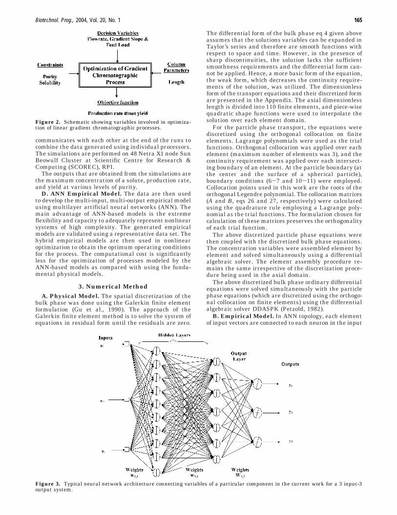
B. Empirical Model. In ANN topology, each elementof input vectors are connected to each neuron in the input

Figure 2. Schematic showing variables involved in optimiza-tion of linear gradient chromatographic processes.

Figure 3. Typical neural network architecture connecting variables of a particular component in the current work for a 3 input-3output system.


layer through the modifiable weights in the weightmatrix wi,j. The inputs to each neuron are summedthrough a summing junction, and the output of eachneuron is obtained by using a sigmoidal transfer function(other transfer functions such as linear, tanh could alsobe used) over the weighted summed input. Finally, theneuron layer outputs are either connected to outputneurons (for a single layer network) or to another layerof neurons in a hidden layer (for multilayer networks).Figure 3 shows the schematic for a two-hidden-layermultilayer perceptron. The case shown is a representa-tive one, having three input and three output vectors.In the output layer, hidden neurons are connected to theoutput vectors. In addition, there is a bias node in eachhidden layer, which is connected to the next layerneurons. Hence, for the particular case shown in Figure3, there are two hidden layers and an output layer. Thefirst and second hidden layers have 10 and 7 neurons,respectively. The transfer function employed for hiddenlayers in the current work is the sigmoidal function, andfor the output layer linear transfer function is utilized.Using linear transfer function in the output layer helpsin estimating the data beyond the range. For clarity, inthe figure bias nodes are not shown. The weight matricesare denoted by wi,j. Here index i and j denote thedestination and source layer, respectively.

The innate problem in neural network is the generali-zation to unseen data. The generalization is essentialbecause generally a training error can be decreased to asmall value; however, for a new data that were not usedto train the network, the error can still be large. Thesimplest way to avoid this overfitting is by increasing thesize of the training set. For many applications, there arelimitations to increasing the data because of economicsand time. Fortunately, this is not an issue in the currentwork since a parallel computing environment is used forthe simulations, and the supply of data is limited onlyto the number of available nodes in the parallel cluster.

To achieve a good generalization, in the current work,increasing the amount of data was not the only mecha-nism adopted. We can find in the literature severalapproaches (e.g., early stopping, regularization, jittering,etc.) to avoid overfitting, each having their own merits.We first explored all the three mentioned approaches;however, after extensive study we found that Bayesianregularization gives better generalization performancethan the early stopping for our system. Hence, in thecurrent work, we have implemented Bayesian regular-ization and jittering to improve generalization. In Baye-sian regularization, both the mean of sum of squares ofnetwork weights and network errors are minimized as

shown in eq 17, and the weights and regularizationparameter (γ) are estimated in an automated fashionusing statistical techniques. The detailed procedure isgiven in MacKay (1992).

In the current work, the data obtained from thephysical model is first preprocessed so that it falls withina [-1, 1] range. The preprocessed data is then dividedinto two data sets, training and test set. The trainingdata set is used to train the network, and the test dataset is used to estimate the generalization error of thenetwork. The high-performance fast training procedure,Levenberg-Marquardt backpropogation, which is basedon nonlinear optimization, is used for training thenetwork. Since it is important for Bayesian regularizationthat the network be trained until sum squared error, sumsquared weights, and the effective number of parametersattain constant values (which essentially indicates thatthe network has attained convergence), the network wastrained until the convergence was achieved. Since theoutputs of the generated networks fall in the [-1, 1]range, the network outputs are postprocessed to convertthe data back into the physical units. All the futureinputs are first preprocessed with the same parameters,which were used to generate the network, and then aresent as input to the network.

The middle eluting component (for the tertiary systemstudied in this paper) generally experiences overlap fromboth the early and later eluting components at higherfeed load conditions. Since the estimated yield andproduction rate may essentially be zero (if purity con-straints are not satisfied), a separate set of simulationswere performed under milder conditions to generateeffective data for modeling the middle eluting component.

4. Results and DiscussionFigure 2 presents the variables involved in a typical

optimization of linear gradient chromatography. Thedecision variables are the parameters over which thedesigner has direct control. For gradient separationsystems these variables are typically flow rate, gradientslope, and feed load. While a wide variety of objectivefunctions have been employed in preparative chromato-graphic separations, the most common objective functionto date has been the production rate, which is defined asthe amount of product produced at a given level of purityper unit time, per unit volume of stationary phase

Table 2. Mass Transfer, Isotherm, and Column and Resin Parameters on FF Sepharose (90 µm)

Mass Transfer Parameters

proteins DP (cm2/s) Ds (cm2/s) 3kf L/R (s-1) ú (cm)

R chymotrypsinogen 2.9 × 10-7 1.45 × 10-8 5 1.5 × 10-2

ribonuclease 3.2 × 10-7 4.8 × 10-8 5 3.3 × 10-2

artificial component 2.5 × 10-7 1.45 × 10-8 5 1.4 × 10-2

Isotherm Parameters

proteins kd (mM-ν/s) KSMA σ ν

R chymotrypsinogen 1.5 × 10-7 0.0039 10 4.4ribonuclease 5.4 × 10-6 0.0077 10 3.7artificial component 2.0 × 10-7 0.0039 10 4.7

Column and Resin Parameters

proteins εi εp εt D (cm) L (cm) Λ

R chymotrypsinogen 0.31 0.68 0.7792ribonuclease 0.31 0.68 0.7792 1.6 10.5 1200artificial component 0.31 0.68 0.7792

MSEREG ) γ1

N∑i)1

N

(ei)2 + (1 - γ)

1

n∑j)1

n

(wj)2 (17)


material. Natarajan et al. (2000) have optimized theproduction rate using yield as a constraint. Although thismethod improves the production rate and satisfies theyield as a hard constraint, it leads to an inflexible setting.In other words, this approach provides minimal flexibilityto the chromatographic engineer who may desire to useyield as a soft constraint. Felinger and Guiochon (1996)suggested using the product of production rate and yieldas an alternative objective function. In this work, we haveemployed the product of production rate and yield as theobjective function. In preparative systems, there are hardconstraints that have to be met to provide a realisticestimate of the achievable production rate of a separation.In the current work, solubility and purity are used as

hard constraints and column length is used as the columndesign parameter. Note: For the simulations in thecurrent work, an initial salt concentration of 50 mM wasemployed. Further, the separation time was determinedby the time required to completely elute the mostretained component.

The transport and kinetic parameters for the proteinsR chymotrypsinogen A and ribonuclease A were obtainedas described previously (Natarajan et al., 2002) and areshown in Figure 2. In that paper, it was demonstratedthat the predictions obtained from the physical modelcorresponded well with the experiments. In the currentarticle, we first investigate the linear gradient separationof a binary model protein mixture (R chymotrypsinogen

Figure 4. Prediction capability of the generated hybrid empirical models for early and later eluting component is shown for totaldata (training and test). Prediction for production rates of early and later eluting components are shown in (a) and (b), respectively.Yield predictions for early and later eluting components are shown in (c) and (d), respectively. Maximum solute concentrationpredictions for early and later eluting components are shown in (e) and (f), respectively.


A and ribonuclease A). To examine a more complexseparation, a ternary mixture consisting of R chymot-rypsinogen A, ribonuclease A, and a later eluting artificialcomponent is then investigated at constant (95%) andvarying (91%, 95% and 99%) levels of purity. Theisotherm and transport parameters of the artificialcomponent is chosen in such a manner that a relativelylow separation factor (1.33) is maintained between themiddle eluting R chymotrypsinogen A and the latereluting artificial component (note: the average separa-tion factor between R chymotrypsinogen A and ribonu-clease A is 1.54). The resulting mass transfer, isotherm,and column parameters for all three components arepresented in Table 2.

Finally, we employ the hybrid modeling approach forsimultaneous optimal column design and identificationof optimal operating conditions at various purity levels.In all of the cases examined in this article, the solubilityconstraint is satisfied using a hard constraint on themaximum solute concentration of 5 mM.

A. Binary Systems. This section presents the opti-mization results for the linear gradient separation of abinary protein mixture (R chymotrypsinogen A andribonuclease A). We first develop the ANN-based hybridmodels for both components as described in the theorysection and then use them in SQP-based optimization.Figure 4 shows that the generated hybrid models haveexcellent predictive ability for outputs (production rate,

Figure 5. Optimization results for two model proteins, R chymotrypsinogen A and ribonuclease A on 90 µm FF Sepharose stationaryphase. Column conditions: diameter 1.6 cm; length 10.5 cm. Feed conditions: ribonuclease A and R chymotrypsinogen A at 0.7 mMeach. ()) Results for early eluting components. (0) Results for later eluting components. All optimal results are presented as a functionof column loadings (DCV). (a) Optimal production rate times yield (mmol/min/mL). (b) Optimal production rate (mmol/min/mL). (c)Optimal yield. (d) Optimal flow rate (mL/min). (e) Optimal gradient slope (mM/DCV). Here DCV, denotes the dimensionless columnvolume.


yield, and maximum solute concentration) of both com-ponents. As seen in the figure, yield data (and cor-respondingly the production rate) was obtained over avery wide range (from 10% to 100%). This ensures theaccurate mapping of the whole design space of interestfor optimization.

Figure 5a illustrates the variation of the optimumproduction rate times yield as a function of feed load forthe early and later eluting components. The correspond-ing optimum values of production rate, yield, gradient

slope and flow rate are shown in Figure 5b-e, respec-tively. Several observations can be made from the figures.The maximum of the production rate times yield for thelater eluting component occurs at a lower column loadingthan that for the early eluting component. In addition,the optimum value of production rate times yield ishigher for the early eluting component than the latereluting component. The corresponding optimal values ofthe production rates are higher for the early elutingcomponent. It can be seen that at higher loadings there

Figure 6. Optimization results for a tertiary mixture (R chymotrypsinogen A, ribonuclease A, and artificial component) on a 90 µmFF Sepharose stationary phase. (0) Results for early eluting component (ribonuclease A). ()) Results for middle eluting component(R chymotrypsinogen A). (3) Results for later eluting component (artificial). Column conditions: diameter 1.6 cm; length 10.5 cm.Feed conditions: ribonuclease A, R chymotrypsinogen A, and the artificial component at 0.5 mM each. The average separation factoris 1.55 between ribonuclease A and R chymotrypsinogen A and 1.35 between R chymotrypsinogen A and the artificial eluting component.All optimal results are presented as a function of column loadings (DCV). (a) Optimal production rate times yield (mmol/min/mL).(b) Optimal production rate (mmol/min/mL). (c) Optimal yield. (d) Optimal flow rate (mL/min). (e) Optimal gradient slope (mM/DCV).


is a relatively sharp decrease in the yield of the latereluting component. In addition, the optimum flow rateis relatively independent of the loading for both early andlater eluting components. The optimal gradient slope firstincreases, then decreases with increased loading, andfinally remains at a constant lower value for higherloadings.

At any feed load, as the gradient slope becomes higher,there is an increased mixed zone between closely retainedcomponents that decreases both the yield and purity ofthe desired component. Under low to moderate feed loadconditions, production rate increases when loading isincreased. At high loading conditions, sample displace-ment effects can become pronounced, resulting in sig-nificant narrowing of the bands. For relatively lowseparation factor systems, any increase in the gradientslope can result in losses of material because the nar-rowing of the bands results in losses due to shock layereffects in these induced sample displacement systems(Nagrath et al., 2002). Hence, increase in the loadingnecessitates lowering of the gradient slope. The optimalflow rate is the highest for all of the loadings becausethe higher production rate attained at higher flow rates

overshadowed any adverse transport effects for thisparticular separation.

B. Tertiary Systems. Tertiary Mixture at a FixedPurity Constraint. To examine a more complex separa-tion, a ternary mixture consisting of R chymotrypsinogenA, ribonuclease A, and a later eluting artificial componentis investigated in this section. We first develop the ANN-based hybrid model for all three components and thenemploy these models in SQP-based optimization. Theoptimization results for all three components are pre-sented in Figure 6. Figure 6a presents the optimal valuesof production rate times yield of the tertiary mixture ata 95% purity constraint. The first component is the earlyeluting ribonuclease A, the second component is R chy-motrypsinogen A, and the third component is the latereluting artificial component. It is important to note thatthe optimal values of the production rate times yield ofthe middle eluting component is below the optimal valuesof the other components, at all levels of loading since itexperiences overlap from both the early and later elutingcomponents. The maximal optimal value of the produc-tion rate times yield of the early eluting componentoccurs at a significantly higher loading than the later

Figure 7. Prediction capability of the generated hybrid empirical models for total data (training and test) at three different puritylevels (91%, 95%, and 99%) for the later eluting component. Prediction for production rates, at 91%, 95%, and 99% purity levels forlater eluting component are shown in (a), (d), and (g), respectively. Yield predictions at 91%, 95%, and 99% purity levels for latereluting components are shown in (b), (e), and (h), respectively. Maximum solute concentration predictions at 91%, 95% and 99%purity levels for later eluting components are shown in (c), (f), and (i), respectively.


eluting component. The optimal production rates of themiddle and later eluting components are lower than thatof the early eluting component. Since the separationfactor between the second and third components isrelatively low, the column loading is restricted to moder-ate values for these components in order to attain higherproduction rates at moderate yields. Further, whilesample displacement effects increase the yield of the earlyeluting component, the effect is less pronounced for thelater eluting component. It is interesting to note thatalthough there is a drop in the optimal production ratevalues at higher and medium loadings for the early andmiddle eluting component, the optimal production rateof the later eluting component is nearly constant athigher loadings. On the other hand, the most significantdecrease of the yield with increased loading is observedfor the later eluting component. The optimal flow ratedecreases with increased loading (from medium to higherloadings) for the middle eluting component as a resultof transport effects at higher loadings. For all of thecomponents, the optimal gradient slope is at the lowestvalue from moderate to high loadings. The increase ofthe optimal gradient slope for the early eluting compo-nent at low loading conditions was observed to be lesspronounced for tertiary systems as compared to binarysystems.

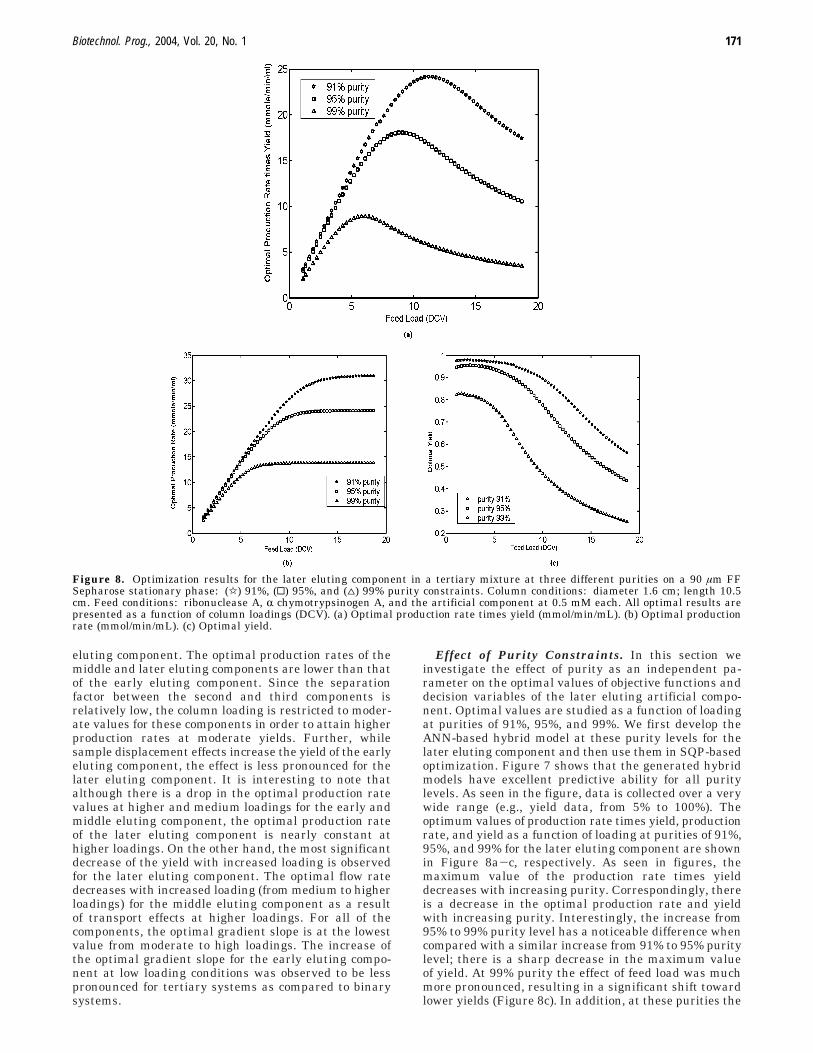
Effect of Purity Constraints. In this section weinvestigate the effect of purity as an independent pa-rameter on the optimal values of objective functions anddecision variables of the later eluting artificial compo-nent. Optimal values are studied as a function of loadingat purities of 91%, 95%, and 99%. We first develop theANN-based hybrid model at these purity levels for thelater eluting component and then use them in SQP-basedoptimization. Figure 7 shows that the generated hybridmodels have excellent predictive ability for all puritylevels. As seen in the figure, data is collected over a verywide range (e.g., yield data, from 5% to 100%). Theoptimum values of production rate times yield, productionrate, and yield as a function of loading at purities of 91%,95%, and 99% for the later eluting component are shownin Figure 8a-c, respectively. As seen in figures, themaximum value of the production rate times yielddecreases with increasing purity. Correspondingly, thereis a decrease in the optimal production rate and yieldwith increasing purity. Interestingly, the increase from95% to 99% purity level has a noticeable difference whencompared with a similar increase from 91% to 95% puritylevel; there is a sharp decrease in the maximum valueof yield. At 99% purity the effect of feed load was muchmore pronounced, resulting in a significant shift towardlower yields (Figure 8c). In addition, at these purities the

Figure 8. Optimization results for the later eluting component in a tertiary mixture at three different purities on a 90 µm FFSepharose stationary phase: (g) 91%, (0) 95%, and (4) 99% purity constraints. Column conditions: diameter 1.6 cm; length 10.5cm. Feed conditions: ribonuclease A, R chymotrypsinogen A, and the artificial component at 0.5 mM each. All optimal results arepresented as a function of column loadings (DCV). (a) Optimal production rate times yield (mmol/min/mL). (b) Optimal productionrate (mmol/min/mL). (c) Optimal yield.


optimum flow rates and optimum gradient slopes arerelatively independent of the loading for the later elutingcomponent (results not shown).

C. Simultaneous Design and Operating Condi-tion Optimization. Tertiary Mixture at a FixedPurity Constraint. To further illustrate the advantageof using a hybrid model framework, it was employed forsimultaneous optimal column design and identificationof optimal operating conditions for the ternary feedmixture. Hybrid models were developed between theoutputs (production rate, yield, and maximum solute

concentration) and inputs (flow rate, gradient slope, feedload, and column length) as described in the theorysection. Figures 9, 10 and 11 present the optimizationresults at 95% purity for the early, middle, and latereluting components, respectively. In the figures, optimalresults are presented as a function of column loadingsand length.

Figure 9 presents the optimal results when productionrate times yield of the early eluting component isoptimized. As seen in Figure 9b, at higher loadingsthe optimal production rate first increases with an

Figure 9. Optimization results as a function of column loadings and column design parameter (length) for an early eluting componentfor a tertiary mixture (R chymotrypsinogen A, ribonuclease A, and the later eluting artificial component on a 90 µm FF Sepharosestationary phase (at 95% puity levels). Column conditions: diameter 1.6 cm. Feed conditions: ribonuclease A, R chymotrypsinogenA, and the artificial component at 0.5 mM each. (a) Optimal production rate times yield (mmol/min/mL). (b) Optimal production rate(mmol/min/mL). (c) Optimal yield. (d) Optimal flow rate (mL/min). (e) Optimal gradient slope (mM/DCV).


increase in length and then decreases when length isincreased beyond its optimal value. The initial increaseof the production rate with an increase in column lengthis due to the increased optimal flow rate with an increasein length. At lower lengths, flow rate has to be decreasedto maintain higher yields. However, when the optimalflow rate reaches its maximum constrained value, anyfurther increase in length causes a decrease of theproduction rate, because of the increased cycle time.For the same reason, at lower column loadings, produc-

tion rate continuously decreases with an increase inlength. Interestingly, at higher loadings yield increaseswith an increase in column length; however, it is es-sentially constant at lower loadings. As mentionedearlier, there is a drop in the optimal flow rate athigher loadings and lower column lengths. The optimalgradient slope is mostly constant at the lowest value,except for lower column lengths and loadings. In general,the optimal values of decision variables for this partic-ular mixture at higher column lengths and loadings

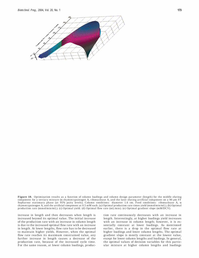
Figure 10. Optimization results as a function of column loadings and column design parameter (length) for the middle elutingcomponent for a tertiary mixture (R chymotrypsinogen A, ribonuclease A, and the later eluting artificial component on a 90 µm FFSepharose stationary phase (at 95% puity levels). Column conditions: diameter 1.6 cm. Feed conditions: ribonuclease A, Rchymotrypsinogen A, and the artificial component at 0.5 mM each. (a) Optimal production rate times yield (mmol/min/mL). (b) Optimalproduction rate (mmol/min/mL). (c) Optimal yield. (d) Optimal flow rate (mL/min). (e) Optimal gradient slope (mM/DCV).


were operation at higher flow rate and low gradientslope.

Figure 10 presents the optimal results when productionrate times yield of the middle eluting component isoptimized. As seen in Figure 10c, to attain a higher yieldat medium to higher loadings for lower to higher columnlengths, the flow rate was decreased from its maximalvalue significantly. Under these conditions, the optimalvalues of the flow rates are lower than when comparedwith the optimization results for the early elutingcomponent. Again, this is because the overlap of the

second component with the other two solutes and thelow separation factor between individual componentslimits the flow rates to moderate values. Interestingly,there is a clear optimal value of production rate andproduction rate times yield at each column length, whichis in sharp contrast to the scenario where the earlyeluting component is optimized. As seen in Figure 9b,optimal production rate experiences only a marginaldecrease at higher loadings and higher lengths for theearly eluting component. As was the case for the earlyeluting component, the optimal gradient slope is constant

Figure 11. Optimization results as a function of column loadings and column design parameter (length) for the later elutingcomponent in a tertiary mixture (R chymotrypsinogen A, ribonuclease A, and the later eluting artificial component on a 90 µm FFSepharose stationary phase (at 95% puity levels). Column conditions: diameter 1.6 cm. Feed conditions: ribonuclease A, Rchymotrypsinogen A, and the artificial component at 0.5 mM each. (a) Optimal production rate times yield (mmol/min/mL). (b) Optimalproduction rate (mmol/min/mL). (c) Optimal yield. (d) Optimal flow rate (mL/min). (e) Optimal gradient slope (mM/DCV).


at the lowest value, except for lower column lengths andloadings. The optimal values of decision variables for thisparticular mixture at higher column lengths and loadingswere operation at medium flow rate and low gradientslope.

Figure 11 presents the optimal results when productionrate times yield of the later eluting component is opti-mized. Interestingly, at higher column lengths the opti-mal production rate first increases with an increase incolumn loading and then remains essentially constantat higher loadings. As seen in the Figure 11b, to maintainhigher production rates at higher column lengths and lowloadings, the optimal gradient slope is maintained athigher values. The optimal values of decision variablesfor this particular mixture at higher column lengths andloadings were operation at high flow rate and lowgradient slope.

The results shown in Figures 9-11 illustrate thesignificant differences in optimal behavior that can occurbetween early, middle, and later eluting components. Itis also important to note that it would be computationallyunreasonable to carry out this class of optimization usingtraditional physical models of preparative chromato-graphic systems.

Effect of Purity Constraints. The effect of purity asan independent design parameter on the simultaneousoptimal column design and identification of optimal

operating conditions was investigated for the later elutingcomponent. Figure 12 presents the optimal resultswhen length was also included as one of the decisionvariables in the optimization. This is in contrast tothe results presented in the previous section (Figures9-11) where length was not included in the decisionvariables for optimization and optimization resultswere presented at various column lengths and loadings.In the current case we can obtain an estimate of theoptimal production rates, yields, flow rates, lengths, andgradient slopes at various levels of column loadings.Hybrid models were developed between the outputs(production rate, yield, and maximum solute concentra-tion) and inputs (flow rate, gradient slope, feed load, andcolumn length) at three levels (91%, 95%, and 99%) ofpurities. In Figure 12, optimal results are shown as afunction of loadings in volume units (mL) in order toillustrate the effect of increased loading due to anincrease in length. This is in contrast to the other resultspresented above where optimal results were shown as afunction of dimensionless loading volume and columnlengths.

As seen in Figure 12d, while higher column lengthsare required to attain higher production rates and yieldsfor 99% purity, the optimal column lengths at lowerpurity levels are at low values. In addition, the optimal

Figure 12. Optimization results for the later eluting component as a function of column loadings (mL) and column design parameter(length, cm), at three different purities for a tertiary mixture (R chymotrypsinogen A, ribonuclease A, and the later eluting artificialcomponent) on a 90 µm FF Sepharose stationary phase. (g) 91%, (0) 95%. and (3) 99% purity constraints. Column conditions: diameter1.6 cm. Feed conditions: ribonuclease A, R chymotrypsinogen A, and the artificial component at 0.5 mM each. (a) Optimal productionrate times yield (mmol/min). (b) Optimal production rate (mmol/min). (c). Optimal yield.


column length first increases and then decreases with acontinuous increase in loadings at 99% purity. Interest-ingly, at lower loadings, optimal yields at 99% purity arehigher than those obtained at 95% purity. At all loadings,the production rate at 95% purity is higher than thatobtained at 99% purity constraint.

To explain the initial increase and decrease of optimalcolumn lengths with an increase in loadings at 99%purity level, we investigate the optimal surface as afunction of column lengths and loadings at 99% purityconstraint. Figure 13 presents the optimal surface resultsfor the later eluting component at various column load-ings and lengths at 99% purity. As seen in Figure 13b,at all loadings, the optimal production rate first increasesand then decreases with a continuous increase in columnlengths. Consequently, in Figure 12d optimal columnlength initially increases with an increase in loadings,to increase the optimal yields. However, it decreaseslater with a further increase in loadings to increasethe optimal production rates. Interestingly, there is aclear difference in the variation of the optimal produc-tion rates with column lengths at 95% and 99% puritylevels. At 95% purity level, optimal production ratecontinuously decreases at all column loadings with anincrease in column lengths, whereas at 99% purity levelthere is a clear optima in column length. In addition, theoptimum flow rates for the later eluting component (at

99% purity level) is a function of lower column lengthsat all loadings.

5. Conclusions and Future Work

In this paper we have developed a hybrid modelframework for optimization of preparative chromato-graphic processes. We have demonstrated that thisstrategy is well suited to address a large number ofdecision variables, permits the exploration of differentdesign scenarios, and enables the straightforward cou-pling of optimal column design with optimal operatingconditions. The hybrid model approach provides flex-ibility to the chromatographic engineer and dramaticallyreduces the computational time required for simulationand multivariable optimization. It also enables theestimation of optimal operating conditions, under differ-ent parametric specifications without any additionalcomputational requirements. We have recently shownthat this strategy is well suited for multiobjective opti-mization (Nagrath et al., 2002), which addresses thepriorities and tradeoffs of various competing objectivesand/or constraints in complex nonlinear chromatographicsystems. Future work will employ this hybrid modelapproach in concert with the GR2R nonlinear controlmethod recently developed by the authors (Nagrath et

Figure 13. Optimization results as a function of column loadings and column design parameter (length) for the later elutingcomponent for a tertiary mixture (R chymotrypsinogen A, ribonuclease A, and the later eluting artificial component on a 90 µm FFSepharose stationary phase (at 99% puity levels). Column conditions: diameter 1.6 cm. Feed conditions: ribonuclease A, Rchymotrypsinogen A, and the artificial component at 0.5 mM each. (a) Optimal production rate times yield (mmol/min/mL). (b) Optimalproduction rate (mmol/min/mL). (c) Optimal yield. (d) Optimal flow rate (mL/min).


al., 2003) for improving the performance of large-scalechromatographic processes by reducing batch-to-batchvariations.

Notationci mobile phase concentration (mM)cfi feed concentration (mM)cp1 pore phase salt concentration (mM)Dai axial dispersion coefficient (cm2/s)Dpi pore diffusion coefficient (cm2/s)Dsi surface diffusion coefficient (cm2/s)kfi film mass transfer coefficient (cm/s)kdi adsorption rate constant (mM-ν/s)kdi desorption rate constant (mM-ν/s)KSMA steric mass action isotherm equilibrium constantL length of column (cm)qi stationary phase concentration (mM)qj1 concentration of bound salt that is not sterically

shielded (mM)q1 total bound concentration of salt on the station-

ary phase (mM)R particle radius (cm)uo interstitial velocity (cm/s)x axial distance (cm)r radial distance inside the particle (cm)

Greek letters

εi interstitial porosityεp particle porosityνi characteristic charge for ith componentσi steric factorΛ ionic capacity (mM)

AppendixA. Dimensionless Equations. Equations 1-11 can

be converted into a nondimensional form using thefollowing dimensionless variables presented in Table 3.

The dimensionless equations for the generalized modelare

The Laplacian ∇s2C used in eq 19 is defined as

where subscript s indicates that the domain is spherical.

where subscript n denotes the component.

Boundary conditions:

B. Bulk Phase Discretized Equations. To derive theweak form of the above eq 18, the differential form isfirst multiplied by a smooth weighting function Wbelonging to a space of functions, W ε Wh

k. The resultingproduct is then integrated over an open space-timedomain Ω. Integration by parts then transfers the spatialderivatives from the fluxes on to the weighting function,thus decreasing the continuity requirements of the solu-tion. In turn boundary integrals appear in the weak form.The weighted residual form of the bulk phase equationcan be written as

where Ω.e is the finite element domain. The integrationby parts of the second order differential terms leads tothe following weak form:

where Cbnh , Wh are interpolated using shape functions

over an element as Cbnh ) ∑A)1

nnp NACbnA , Cbn,i

h ) ∑A)1nnp NA,i

CbnA , and Wh ) ∑A)1

nnp NADA. Since the interpolating func-tions are chosen to be same for both the solution andweight space, it leads to a Galerkin form. After substitut-ing Cbn

h , Wh with the interpolating functions, a set ofnonlinear ordinary differential equations are obtainedwhich in the matrix form can be expressed as

C. Particle Phase Discretized Equations. Usingorthogonal collocation on finite elements the above equa-

Table 3. Dimensionless Variables Formed for the General Rate Model

τ ) t / L/u0 z ) x / L ê ) r / R Cbi ) cbi / Cfi Cpi ) cpi / Cfi

Φki ) (1 - εp)qmax i / εpCfi Pei ) u0L / Dai Bfi ) kfiL / εpRu0

Nfi ) 3L / R (1 - εb)kfi / εbu0 Npi ) DpiL / u0R2 Nsi ) DsiL / u0R

2

Yli ) yliL / qmaxiu0

∂Cbi

∂τ) 1

Pei

∂2Cbi

∂z2-

∂Cbi

∂z- Nfi[Cbi - Cpi(ê ) 1)] (18)

∂Cpi

∂τ) Npi∇s

2Cpi - ΦkiYli (19)

∇s2C ) 1

z2∂

∂(z2∂C∂z )

Ki

∂θi

∂τ) KiNsi∇θi + ΦkiYli (20)

∂Cbi

∂z) [Pei[Cbi - Cfi] z ) 0

0 z ) 1 ] (21)

Npi

∂Cpi

∂ê+ KiNsi

∂θi

∂ê) ⟨Pei[Cpi - Cfi] ê ) 1⟩

2KiNsi

∂θi

∂ê) Ki

∂θi

∂τ- ΦkiYliê ) 1 (22)

∫Ωe Wh(∂Cbn

∂τ- 1

Pen

∂2Cbn

∂z2+

∂Cbn

∂z+ Nfn[Cbn -

Cpn(ê ) 1)])dΩe ) 0 (23)

∫Ωe WhCbn,th + 1

Pen∫Ωe W,i

h Cbn,ih dΩe - 1

PenWhCbn,i

h |Γe +

∫Ωe (WhCbn,ih + NfnWhCbn

h )dΩe -

∫Ωe NfnWhCpn(ê ) 1)dΩe ) 0 (24)

[Mn][C′bn] ) [Kn][Cbn] + [Bn] + [Fn]Cpn(ê ) 1) (25)


tions are discretized for element l and collocation point ias

For the l th element,

The discretized boundary conditions for the pore and thesolid phase can be represented as

Boundary conditions:

References and Notes(1) Brooks, C. A.; Cramer, S. M. Steric mass-action ion-

exchange: Displacement profiles and induced salt gradients.AIChE J. 1992, 38(12), 1969-1978.

(2) Ernest, M. V.; Whitley, R. D., Jr.; Ma, Z.; Wang, N.-H. L.Effects of mass action equilibria on fixed-bed multicomponention exchange dynamics. Ind. Eng. Chem. Res. 1997, 36(1),212-226.

(3) Felinger, A.; Guiochon, G. Comparison of maximum produc-tion rates and optimum operating/design parameters inoverloaded elution and displacement chromatography. Bio-technol. Bioeng. 1993, 41, 134-147.

(4) Felinger, A.; Guiochon, G. Optimizing experimental condi-tions in overloaded gradient elution chromatography. Bio-technol. Prog. 1996, 12(5), 638-644.

(5) Gallant, S. R.; Kundu, A.; Cramer, S. M. Optimization ofstep gradient separations: Consideration of nonlinear ad-sorption. Biotechnol. Bioeng. 1995, 47(3), 355-372.

(6) Gallant, S. R.; Vunnum, S.; Cramer, S. M. Optimization ofpreparative ion-exchange chromatography of proteins: Lineargradient separations. J. Chromatogr. A 1996, 725(2), 295-314.

(7) Guiochon, G.; Golshan-Shirazi, S.; Katti, A. M. Fundamen-tals of Preparative and Nonlinear Chromatography; AcademicPress: New York 1994.

(8) Gu, T.; Tsao, G. T.; Ladisch, M. R. Displacement effect inmulticomponent chromatography. AIChE J. 1990, 36(8),1156-1162.

(9) Luo, R. G.; Hsu, J. T. Optimization of gradient profiles inion-exchange chromatography for protein purification. Ind.Eng. Chem. Res. 1997, 36, 444-450.

(10) Ma, Z.; Whitley, R. D.; Wang, N.-H. L. Pore and surfacediffusion in multicomponent adsorption and liquid chroma-tography systems. AIChE J. 1996, 42(5), 1244-1262.

(11) MacKay, D. J. C. Bayesian interpolation. Neural Comput.1992, 4, 415-447.

(12) Nagrath, D.; Messac, A.; Bequette, B. W.; Cramer, S. M.Physical programming based multiobjective optimizationstrategies for chromatographic processes. AIChE J. 2002,submitted for publication.

(13) Nagrath, D.; Bequette, B. W.; Cramer, S. M. Evolutionaryoperation and control of chromatographic processes. AIChEJ. 2003, 49(1), 82-95.

(14) Natarajan, V.; Cramer, S. M. Modeling shock layers in ion-exchange displacement chromatography. AIChE J. 1999b,45(1), 27-37.

(15) Natarajan, V.; Bequette, B. W.; Cramer, S. M. Optimizationof ion-exchange displacement separations I. Validation of aniterative scheme and its use as a methods development tool.J. Chromatogr. A 2000, 876(1-2), 51-62.

(16) Natarajan, V.; Cramer, S. M. A Methodology for thecharacterization of ion-exchange resins. Sep. Sci. Technol.2000a, 35(11) 1719-1742.

(17) Natarajan, V.; Cramer, S. M. Optimization of ion-exchangedisplacement separations II. Comparison of displacementseparations on various ion-exchange resins. J. Chromatogr.A 2000b, 876(1-2), 63-73.

(18) Natarajan, V.; Ghose, S.; Cramer, S. M. Comparison oflinear gradient and displacement separations in ion-exchangesystems. Biotechnol. Bioeng. 2002, 78(4) 365-375.

(19) Petzold, L. R. DASSL: A Differential/Algebraic SystemSolver; Lawrence Livermore National Laboratory: Livermore,CA, 1982.

(20) Saunders, M. S.; Vierow, J. B.; Carta, G. Uptake ofphenylalanine and tyrosine by a strong-acid cation exchanger.AIChE J. 1989, 35(1), 53-68.

(21) Suwondo, E.; Wilhelm, A. M.; Pibouleau, L.; Domenech,S. Optimization of a liquid chromatographic separationprocess. Comput. Chem. Eng. 1993, 17, S135-S140.

(22) Yoshida, H.; Yoshikawa, M.; Kataoka, T. Parallel transportof BSA by surface and pore diffusion in strongly basicchitosan. AIChE J. 1994, 40(12), 2034-2044.

Accepted for publication September 5, 2003.

BP034026G

dCpn,i

dτ) Npi

1

hl ∑

j)1

NCOL+2

Bi,jCpn,j +2

rl∑j)1

NCOL+2

Ai,jCpn,j +

ΦknYln,i (26)

Kn,i

dθn,i

dτ) KnNsn,i ∑

j)1

NCOL+2

Bi,jθn,j +2

rl∑j)1

NCOL+2

Ai,jθn,j +

ΦknYln,i (27)

rl )ê - êl

hlhl ) êl+1 - êl

Npi

∂Cpi

∂ê+ KiNsi

∂θi

∂ê) ⟨Pei[Cpi - Cfi]; ê ) 1⟩

2KiNsi

∂θi

∂ê) Ki

∂θi

∂τ- Φki Yli; ê ) 1

∑NCOL+2

j)1

AijCpn,j ) 0 ⟨ε ) 0|

∑NCOL+2

j)1

AijCpn,j ) 0 ⟨ε ) 0| (28)


a hybrid model framework for the optimization of … hybrid model framework for the optimization of...

Documents