hybrid simulation-optimization based approach for the
TRANSCRIPT
Hybrid Simulation-Optimization basedapproach for the Optimal Design of
Single-Product Biotechnological Processes
Robert Brunet1, Gonzalo Guillen-Gosalbez1∗, J. Ricardo Perez-Correa2,Jose Antonio Caballero3 and Laureano Jimenez1
1 Departament d’Enginyeria Quimica, Escola Tecnica Superior d’Enginyeria Quimica,
Universitat Rovira i Virgili, Campus Sescelades, Avinguda Paisos
Catalans 26, 43007, Tarragona, Spain
2 Departamento de Ingenieria Quimica y Bioprocesos, Pontificia Universidad
Catolica de Chile, Casilla 306, Correo22, Santiago de Chile, Chile
3 Departmento de Ingenieria Quimica, Universidad de Alicante,
Aparatado de Correos 99. 03080 Alicante, Spain
∗Corresponding author. E-mail: [email protected], telephone: +34 977558618
1
brought to you by COREView metadata, citation and similar papers at core.ac.uk
provided by Repositorio Institucional de la Universidad de Alicante

Abstract
In this work, we present a systematic method for the optimal development of bio-
processes that relies on the combined use of simulation packages and optimization
tools. One of the main advantages of our method is that it allows for the simultane-
ous optimization of all the individual components of a bioprocess, including the main
upstream and downstream units. The design task is mathematically formulated as a
mixed-integer dynamic optimization (MIDO) problem, which is solved by a decom-
position method that iterates between primal and master sub-problems. The primal
dynamic optimization problem optimizes the operating conditions, bioreactor kinet-
ics and equipment sizes, whereas the master levels entails the solution of a tailored
mixed-integer linear programming (MILP) model that decides on the values of the in-
teger variables (i.e., number of equipments in parallel and topological decisions). The
dynamic optimization primal sub-problems are solved via a sequential approach that
integrates the process simulator SuperPro Designer with an external NLP solver im-
plemented in Matlab. The capabilities of the proposed methodology are illustrated
through its application to a typical fermentation process and to the production of the
amino acid L-lysine.
Keywords: hybrid simulation-optimization; mixed-integer dynamic optimization; biotech-
nological processes; L-lysine.
2

1 INTRODUCTION
Because of their potential to produce high-value products in human health and care, biopro-
cesses have recently gained wider interest. The recent boost in competitiveness for customers
and new products experienced in this sector has created a clear need for modeling and op-
timization tools to assist decision-makers in the early stages of the process development.
A bioprocess is a special type of chemical process that produces biochemical products (e.g.
antibiotics, proteins, amino acids, etc.) from microorganisms or enzymes. Bioprocesses share
some common features with general chemical processes, but differ in their kinetics of prod-
uct formation, process structure (unit operations and procedures) and operating constraints
(Heinzle et al. 2006a).
Optimization approaches devised so far in biotechnology have primarily focused on the
bioreactor step. Cuthrell and Biegler (1989) optimized a fed-batch reactor for penicillin
production with a solution strategy based on successive quadratic programming (SQP) and
orthogonal collocation on finite elements. Carrasco and Banga (1997) addressed the dy-
namic optimization of batch and fed-batch reactors using stochastic optimization algorithms.
More recently, Banga et al. (2005) introduced a new solution method for this problem based
on control parameterization, whereas Sarkar and Modak (2005) proposed the use of genetic
algorithms in this context. For an extensive review of dynamic optimization of bioreactors,
the reader is referred to Banga et al. (2003).
Another area related with the bioreactor step that has received attention in the literature
is the optimization of metabolic networks. Raghunathan et al. (2003) addressed the data
reconciliation and parameter estimation problems in metabolic networks, whereas Guillen-
Gosalbez and Sorribas (2009) and Pozo et al. (2010) have proposed deterministic global
optimization techniques for kinetic models of metabolic networks that assist in biotechno-
logical and evolutive studies.
In contrast to these approaches, the optimization of complete bioprocesses considering all
their individual steps has received very little attention to date. This can be attributed to
3

the fact that these problems lead to complex formulations that integrate structural and op-
erating decisions, some of which change over time. To the best of our knowledge, the work
by Groep et al. (2000), is the only one that addressed the optimization of a entire bioprocess
(i.e., production of an intracellular enzyme alcohol dehydrogenase). This pioneering work
has two main limitations: (i) it assumed a fixed plant topology; and (ii) it applied a simple
sensitivity analysis to optimize the operating variables of the process that is not guaranteed
to converge to a local (or global) optimum.
Hence, it seems clear that the rich theory available for synthesizing standard chemical pro-
cess flowsheets has not been applied to the same extent to their biochemical counterparts.
In fact, the design of bioprocess flowsheets is nowadays typically accomplished by empirical
and/or intuitive methods such as rules of thumb or simple heuristics (Petrides et al. 1996,
Koulouris et al. 2000, Wong et al. 2004 and Petrides et al. 2006) that are likely to lead to
sub-optimal process alternatives.
With this observation in mind, the aim of this paper is to present a systematic tool for the
design of bioprocesses that relies on the combined use of simulation and optimization tech-
niques. More precisely, the design task is formulated as a mixed-integer dynamic optimiza-
tion (MIDO) problem, which is solved by a hybrid simulation-optimization decomposition
method that exploits the complementary strengths of optimization tools (i.e., nonlinear pro-
gramming, NLP, and mixed-integer linear programming, MILP) and commercial bioprocess
simulators (i.e., SuperPro Designer). Our methodology has been tested using two different
examples: a typical fermentation process and the production of the amino acid L-Lysine.
2 PROBLEM STATEMENT
The problem addressed in this article can be formally stated as follows. Given are the demand
and prices of final products, cost parameters, including capital investment and operating cost
data (i.e., raw materials and utilities cost), time horizon, thermodynamic properties and per-
4

formance models of the equipment units embedded in the flowsheet, including the bioreactor
kinetics. The goal of the analysis is to determine the optimal process design, including type
and size of process units (e.g., centrifuge, decanter, filtration, etc.), number of equipment
units in parallel and operating conditions (concentrations, flow rates, temperatures, etc.)
that maximize a given economic performance indicator over a specified time horizon.
In this work, we consider single-product batch plants that can operate with more than one
equipment unit (in parallel) per stage. The equipment units in parallel are assumed to be of
the same size and operating under the same process conditions. The unit yields are described
through nonlinear process models that may require the solution of differential-algebraic equa-
tions (DAEs). The operating times and batch sizes are regarded as continuous variables to be
optimized rather than as fixed parameters. It should be emphasized that many bioprocesses
follow this general pattern, such as the production of penicillin, citric and pyruvic acid,
vitamin riboflavin, human serum and insulin, monoclonal antibodies, and plasmid DNA,
among many others. It is also important to clarify that in this work the emphasis is on the
optimization of the operating conditions and topology of these processes, rather than on the
solution of the scheduling problem associated with complex bioprocess batch facilities. The
reader is referred to the review paper by Mendez et al. (2006) for more details on general
scheduling approaches, the overwhelming majority of which assume fixed operating times
and process yields.
3 MATHEMATICAL FORMULATION
Most bioreactors in commercial bioprocesses operate in batch or fed-batch mode. Thus,
the reaction kinetics of the biochemical conversions, catalysed either by single enzymes or
by cells, are the cornerstones of a bioprocess synthesis problem. The design task requires
therefore the simultaneous solution of a mixed-integer non-linear programming (MINLP)
synthesis models with embedded DAEs. This gives rise to mixed-integer dynamic optimiza-
5

tion (MIDO) problems, the solution of which is a highly difficult task (Bansal et al. 2003).
So far, MIDO algorithms have been applied to the integrated design and control of process
plants (Pistikopoulos et al. 2004), simultaneous scheduling and optimal control of reactors
(Terrazas-Moreno et al. 2007) and optimization of hybrid systems (Allgor and Barton 1999).
However, to our knowledge, they have never been applied to the optimization of a complete
biotechnological process model.
In mathematical terms, the synthesis of biotechnological processes can be posed as a MIDO
problem. In this work, we apply the following notation taken from Bansal et al. (2003),
which may be simplified in some cases according to the features of the design problem being
addressed.
minu(t),d,y
J(xd(tf ), xd(tf ), xa(tf ), u(tf ), d, y, tf )
s.t. hd(xd(t), xd(t), xa(t), u(t), d, y, t) = 0 ∀t ∈ [t0, tf ]
ha(xd(t), xa(t), u(t), d, y, t) = 0 ∀t ∈ [t0, tf ]
h0(xd(t0), xd(t0), xa(t0), u(t0), d, y, t0) = 0
hp(xd(ti), xd(ti), xa(ti), u(ti), d, y, ti) = 0 ∀ti ∈ [t0, tf ] i = 1, ..., I
gp(xd(ti), xd(ti), xa(ti), u(ti), d, y, ti) ≤ 0 ∀ti ∈ [t0, tf ] i = 1, ..., I
hq(d, y) = 0
gq(d, y) ≤ 0
(1)
In this formulation, hd = 0 and ha = 0 represent the set of differential-algebraic equations
(DAEs) that describe the dynamic system whose initial conditions are h0 = 0. hp = 0 and
gp ≤ 0 enforce conditions that must be satisfied at specific time instances, whereas hq = 0
and gq ≤ 0 are time invariant equality and inequality constraints, respectively. xd(t) and
xa(t) denote the differential state and algebraic variables of the dynamic system, u(t) is the
vector of time-varying control variables, d is the vector of time-invariant continuous search
variables and y are the binary variables, which in our case are assumed to be time invariant.
6

Note that the embedded DAE system is required in order to model the bioreactor kinetics.
The binary variables are necessary for representing the different topological decisions, such as
the number of equipment units in parallel or the selection of different alternative units in the
process. The vector y of binary variables contains M·N components, where M represents the
different types of process units and N the maximum number of equipment units in parallel.
The component ym,n of this vector takes the value of 1 if n equipment units in parallel of
type m are selected, and 0 otherwise. Note that the logical relationships among the binary
variables describing connections and interactions between the units in the superstructure are
expressed also via constraints hq = 0.
There are currently two major approaches to solve MIDO problems. The first type relies on
converting the MIDO problem into a finite-dimensional MINLP by complete discretization
using techniques such as orthogonal collocation on finite elements (Balakrishna and Biegler,
1993). The resulting MINLP can then be solved by classical MINLP methods. The second
class of MIDO algorithms, to which the strategy presented in this work belongs, is based
on the use of reduced space methods (Allgor and Barton, 1999). These techniques rely on
decomposing the problem into a series of primal dynamic optimization sub-problems with
fixed binary variables, and master MILP sub-problems that predict new values of the binary
variables for the primal sub-problems.
In complete discretization approaches, the MINLP resulting from the discretization tends to
be very large even for relatively small problems, as this approach requires a large number of
variables and constraints in order to approximate the solution of the DAE system. On the
other hand, in reduced space methods, the difficulty arises in the definition of the master
MILP sub-problem. This master problem is typically created by either approximating the
nonlinear objective function and constraints by first order linearizations (i.e., supporting
hyperplanes) or by deriving Benders cuts from the solution of the primal problem and as-
sociated dual information. In the section that follows, we introduce a customized reduced
space method for the solution of MIDO problems arising in the design of bioprocesses that
7

integrates optimization tools with a bioprocess simulator.
4 SOLUTION PROCEDURE
The solution strategy developed in this work is a reduced space method inspired by the
works by Diwekar et al. (1992), Kravanja and Grossmann (1996) and Caballero et al. (2005).
The key ideas of the approach presented are: (i) to integrate mathematical programming
tools with a standard bioprocess simulator in the context of a reduced space method for
MIDOs; and (ii) to derive a tailored master MILP formulation that exploits the structure of
the problem.
The proposed algorithm iterates between master and primal sub-problems, as shown in
Figure 1. The primal level entails the solution of a dynamic nonlinear programming sub-
problem, in which the integer decisions, mainly the number of equipments in parallel, are
fixed. As discussed in section 5, the solution of this sub-problem requires calculations per-
formed by the bioprocess simulator. On the other hand, the task of the customized master
problem is to decide on the value of the integer variables. The algorithm solves iteratively
both sub-problems until a termination criterion is satisfied. A stopping criterion that tends
to work very well in practice consists of stopping as soon as the primal sub-problems start
worsening (i.e. the current primal sub-problem yields an optimal objective function that
is worse than the previous one). The main features of these sub-problems are described in
detail in the next sub-sections.
(Figure 1 could be placed here)
8

4.1 Primal sub-problem
The primal level entails the solution of a dynamic optimization problem at iteration k of the
algorithm for fixed values of the binary variable k:
minu(t),d,y
J(xd(tf ), xd(tf ), xa(tf ), u(tf ), d, y, tf )
s.t. hd(xd(t), xd(t), xa(t), u(t), d, y, t) = 0 ∀t ∈ [t0, tf ]
ha(xd(t), xa(t), u(t), d, y, t) = 0 ∀t ∈ [t0, tf ]
h0(xd(t0), xd(t0), xa(t0), u(t0), d, y, t0) = 0
hp(xd(ti), xd(ti), xa(ti), u(ti), d, y, ti) = 0 ∀ti ∈ [t0, tf ] i = 1, ..., I
gp(xd(ti), xd(ti), xa(ti), u(ti), d, y, ti) ≤ 0 ∀ti ∈ [t0, tf ] i = 1, ..., I
hq(d, y) = 0
gq(d, y) ≤ 0
(2)
In the context of our algorithm, this primal sub-problem is solved by parameterizing the
control variables, u(t) , in terms of time-invariant parameters (reduced space discretisation
or control vector parameterisation). Then, for given u(t) and values of the remaining search
variables, d (e.g., equipment sizes, operating conditions, etc.) the DAE system is integrated
by the process simulator, which in addition to solving the bioreactor kinetics, it calculates
mass and energy balances and key economic parameters of the entire process. As will be
discussed later on, in some cases it might be necessary to introduce an intermediate module
that couples the model implemented in the bioprocess simulator with an external ODE solver
algorithm (e.g., implicit Runge-Kutta method). This allows dealing with complex kinetic
models that cannot be directly implemented in the process simulator. An external NLP
solver is finally employed for searching the values of the control and design variables that
maximize the NPV. To accomplish this task, it is necessary to obtain gradient information
with respect to the objective function and constraints through finite difference perturbations.
9

(Figure 2 could be placed here)
Figure 2 outlines the solution procedure of the primal sub-problem. One of the main advan-
tages of the approach presented is that it benefits from the unit operations models already
implemented in the bioprocess simulator, which avoids having to define them in an explicit
form (i.e., equation oriented). This issue facilitates to a large extent the implementation
step, as it allows optimizing bioprocess models that are already implemented in the simu-
lator without having to define the associated process and economic equations in an explicit
way.
Note that due to the structure of the implicit models in a process simulator, the equations
hq(d, y) = 0 are eliminated by expressing dependent variables z in terms of decision vari-
ables v, that is hq(v, z, y) = 0 ⇒ z = ϕq(v). Therefore, the NLP subproblem as it arises in
a process simulator for fixed binary variables is indeed given as follows:
minu(t),d,y
J(xd(tf ), xd(tf ), xa(tf ), u(tf ), v, ϕ(v), y, tf )
s.t. hd(xd(t), xd(t), xa(t), u(t), v, ϕ(v), y, t) = 0 ∀t ∈ [t0, tf ]
ha(xd(t), xa(t), u(t), v, ϕ(v), y, t) = 0 ∀t ∈ [t0, tf ]
h0(xd(t0), xd(t0), xa(t0), u(t0), v, ϕ(v), y, t0) = 0
hp(xd(ti), xd(ti), xa(ti), u(ti), v, ϕ(v), y, ti) = 0 ∀ti ∈ [t0, tf ] i = 1, ..., I
gp(xd(ti), xd(ti), xa(ti), u(ti), v, ϕ(v), y, ti) ≤ 0 ∀ti ∈ [t0, tf ] i = 1, ..., I
hq(v, ϕ(v), y) = 0
gq(v, ϕ(v), y) ≤ 0
(3)
A very important point in the method is that the process simulator must converge at each
time the solver sends a set of values for the design variables. Otherwise the overall procedure
will fail. One way to ensure convergence consists of adding slack variables and a penalty to
10

the objective function (Viswanathan and Grossmann 1990). This gives rise to the following
primal sub-problem:
minu(t),d,y
J(xd(tf ), xd(tf ), xa(tf ), u(tf ), v, ϕ(v), y, tf )
+∏T (s+hp + s−hp + sgp + s+hq + s−hp + sgq)
s.t. hd(xd(t), xd(t), xa(t), u(t), v, ϕ(v), y, t) = 0 ∀t ∈ [t0, tf ]
ha(xd(t), xa(t), u(t), v, ϕ(v), y, t) = 0 ∀t ∈ [t0, tf ]
h0(xd(t0), xd(t0), xa(t0), u(t0), v, ϕ(v), y, t0) = 0
hp(xd(ti), xd(ti), xa(ti), u(ti), v, ϕ(v), y, ti) + s+hp − s−hp = 0 ∀ti ∈ [t0, tf ] i = 1, ..., I
gp(xd(ti), xd(ti), xa(ti), u(ti), v, ϕ(v), y, ti)− sgp ≤ 0 ∀ti ∈ [t0, tf ] i = 1, ..., I
hq(v, ϕ(v), y) + s+hp − s−hp = 0
gq(v, ϕ(v), y)− sgq ≤ 0
(4)
where∏
is a penalty parameter vector whose value is finite but chosen to be sufficient large,
whereas s+hp, s−hp, sgp, s
+hq, s
−hp and sgq are vectors of positive variables.
4.2 4.2. Master sub-problem
The goal of the master problem is to provide a new set of values for the binary variables that
yield better results than the previous one. Here, we present a tailored master MILP that
exploits the structure of the problem. Note that due to the presence of nonconvexities in
the model, it is not guaranteed that this master MILP will provide a rigorous lower bound
on the global optimal solution of the problem.
To generate the master MILP, the design variables are fixed to the optimal value obtained
in the latest NLP solved at iteration k of the algorithm, and a series of simulation problems
are calculated. The master MILP takes the following form:
11

minu(t),d,y
η +ΠT (sgp + shq + sgq)
s.t. η ≥ Jk +
(∂J
∂v
)|k (v − vk) +
∑j
(∂J
∂uj
)|k (uj − uj
k) + ∆Jk · y
0 ≥ T kp
{hkp +
(∂hp
∂v
)|k (v − vk) +
∑j
(∂hp
∂uj
)|k (uj − uk
j ) + ∆hkp · y
}sgp ≥ gkp +
(∂gp∂v
)|k (v − vk) +
∑j
(∂gp∂uj
)|k (uj − uj
k) + ∆gkp · y
shq ≥ T kq
{hkq +
(∂hq
∂v
)|k (v − vk) + ∆hk
q · y}
sgq ≥ gkq +
(∂gq∂v
)|k (v − vk) + ∆gkq · y
T kp =
−1 if λk
p < 0
0 if λkp = 0
1 if λkp > 0
T kq =
−1 if λk
q < 0
0 if λkq = 0
1 if λkq > 0
(5)
The objective function is formed by the auxiliary variable η and a penalty for constraint
violation Π that multiplies the slack variables. The linearizations of the objective function
and time variant constraints contain three main terms corresponding to: the design variables
(vk), control variables (ujk) and the binary variables representing the topological alternatives
(y). Note that the control variables uj are parameterized by means of a piecewise constant
profile defined on J sub-intervals. On the other hand, the time invariant constraints only
consider, the design and topological decisions. In this formulation, λkp and λk
q represent the
Lagrangean multipliers associated with the time-invariant and time-variant equality con-
straints, respectively, of the NLP solved at in iteration k of the algorithm. These values are
used to correctly relax the equalities into inequalities.
A key issue in this master MILP is how to obtain the derivatives of the objective function
and constraints with respect to the decision variables. The derivatives of the continuous
variables are approximated by perturbing them in the optimal solution of the NLP problem.
12

On the other hand, the partial derivatives with respect to the binary variables, which do not
appear explicitly in the MIDO formulation, are determined by running several simulations
for different topologies. Note that at each iteration, we need the derivatives of the objec-
tive function and the constraints with respect to all the components ym,n of the vector of
binary variables. This requires performing at most (depending on the allowable interconec-
tions between the equipment units) M·N-1 simulations, in each of which we concentrate on
changing one single process unit, while keeping the remaining topological decisions fixed.
More precisely, we select one process unit m at a time, and run several simulations, each
corresponding to a different number n of equipment units in parallel (i.e., from zero, the
unit does not exist, up to the maximum number of equipment units in parallel) and leav-
ing the remaining topological decisions unchanged. In performing this step, we discard two
types of topological alternatives: (i) those that violate the logical relationships among the
binary variables describing allowable connections and interactions between the units, which
are expressed via constraints hq = 0; and (ii) those that are likely to lead to sub-optimal
alternatives. To identify topologies of type (ii), we apply a heuristic rule that removes those
process alternatives that place equipments in parallel in units others than the bottleneck of
the topology found in iteration k. Note that all these simulations can be performed very effi-
ciently because the starting point is the optimal solution of the NLPk. Note that to keep the
production rate constant in all the simulations, which allows for a fair comparison between
the different alternatives being assessed, it is necessary to adjust the input flow rates to the
units according to the yields and number of equipment units in parallel. This step can be
easily performed with the process simulator assuming that all the process yields remain the
same as in the optimal solution of the NLP solved in the previous iteration of the algorithm.
It should be noted that all the linear constraints are accumulated in the master MILP, this
means that at iteration k, the problem includes the constraints generated at the kth iteration
plus all the constraints of all previous iterations. In all cases, after determining the new set of
values of the binary variables, the primal problem is solved again, and the overall procedure
13

is repeated until the termination criterion is satisfied.
4.3 Remarks
• At this point, time varying binary variables are not considered.
• All the required parameters to simulate the bioprocess are initialized in the simula-
tor environment (i.e., properties of the components, equipment parameters, economic
parameters, etc.). Also, the number of equipment units in parallel must be specified
every time the simulation model is solved.
• The problem addressed in this work can be seen as a special case of the design of
single product multi-stage batch plants (see Biegler et al. 1997). Note, however, that
in standard scheduling formulations the operating times are assumed to be constant
and the process models linear, whereas our approach accounts for variable operating
times and nonlinear process models, including the kinetics of the bioreaction.
• Integer cuts can be added to the master problem in order to avoid the repetition of
solution explored so far in the primal problem.
• Note that in each iteration of the algorithm we generate linearizations for the process
models of both, the existing and non-existing equipment units.
5 RESULTS
The capabilities of the proposed approach are illustrated through two case studies. The
implementation of the overall method is discussed in first place, whereas the case studies are
described next.
14

5.1 Computer architecture / implementation
The model of the biotechnological plant is developed using SuperPro Designer, (Intelligen,
NJ), a process simulation tool in which the mass and energy balances as well as the calcula-
tion of the key economic indicators are implemented. Note, however, that any other process
simulator could be used for the same purpose.
The capabilities of this process simulator are enhanced by coupling it with a dynamic model
of the bioreactor coded in Matlab and connected with SuperPro Designer, using the Com-
ponent Object Module (COM) technology implemented in the Pro-Designer COM Server.
The kinetic model of the bioreactor is solved by the odefun function of Matlab. Most of
the problems are solved using ode45, which is based on an explicit Runge-Kutta formula,
the Dormant-Prince Pair (Forsythe et al. 1977). For stiff problem, the ode15s algorithm
(Shampine, 1994) can be employed.
As NLP solvers, we use the fmincon function that implements a sequential quadratic pro-
gramming (SQP) method. The Hessian of the Lagrangian is updated using the BFGS formula
(Powell, 1978). The master MILP is implemented in GAMS and solved with CPLEX. The
termination criterion applied in the numerical examples is the NLP worsening (i.e., the al-
gorithm stops when the NLPs start to deteriorate). In order to communicate both software
packages, we use the interface GAMS-Matlab developed by Ferris (2010).
Note that the function fmincon minimizes a given objective function. In our case, we reverse
the sign of the NPV in order to pose the problem as a minimization one.
5.2 Case Study I. A basic fermentation process
We first consider a basic illustrative example of a hypothetical fermentation process (Figure
3). The process includes two steps: a reaction that takes place in a fermentor, and a separa-
tion that is performed in either a decanter, a centrifuge or a filter. In the reaction-phase, the
initial substrate dissolved in water reacts with oxygen forming product A and by-products
(waste). In the second stage, the product is separated to obtain pure A. The production
15

recipe involves the following operations: charge of water (time neglected), charge of sub-
strate (time neglected), heating (60 min), charge of inoculum (time neglected), fermentation
(time to be optimized), cooling (60 min) and transfer out (time neglected) carried out in the
reactor; and a separation task whose time depends on the equipment used (decanting 120
min, centrifugation 100 min, and filtration 130 min).
Substrate and water are charged at 25oC. Then the mixture is heated until the optimal
growth temperature (i.e., 37oC) using steam at 152oC, with an efficiency of 80% in the heat
transfer. The inocolum is added when the optimal temperature is reached. The reaction is an
aerobic fermentation carried out at constant temperature that is modeled by a Monod-type
kinetics of the following form:
µ = µmaxS
KM+S(6)
where µ is the rate of formation of biomass expressed in g/l·h, S is the concentration of
substrate in g/l and KM and µmax are kinetic parameters that take a value of 0.2 h−1 and 35
g/l, respectively. The reaction requires an aeration stream of 0.5 VVM (i.e., volume of air
per volume of liquid per min). Chilled water is used to remove the metabolic heat (reaction
enthalpy equals -15,478 kJ/kg). The stoichiometry of the reaction is as follows:
100 kg Substrate + 70 kg O2 → 28 kg Biomass + 70 kg CO2 + 60 kg H2O + 2 kg A + 10
kg waste
The final mixture is cooled down to 25oC, using chilled water and assuming an efficiency
of 90% in the heat transfer. The mixture is then transferred to the separation equipment,
where a percentage of A is separated from the remaining compounds yielding a final product
with a purity of 100%. The efficiency in the decanter and filter is 90% (i.e., 90% of A is
16
retained and 10% is lost), whereas that of the centrifuge is 92%.
(Figure 3 could be placed here)
The design objective is to maximize the NPV assuming a fixed demand of 2025 kg/year
of A. The entire process is modeled using SuperPro Designer, the kinetic model and the
NLP solver are implemented in Matlab, whereas the master MILP is coded in GAMS. The
bioreactor is modeled as a stoichiometric reactor in SuperPro Designer, whose conversion is
provided by Matlab after integrating the DAE system that describes the kinetic model. The
NLP solver is also implemented in Matlab, whereas the master MILP is solved with CPLEX
interfacing with GAMS. As NLP solver, we use a gradient based method (i.e., SQP). The
continuous decision variables to be optimized are the initial substrate concentration and the
reaction time. The integer decision variables represent the number of equipment units in
parallel, as well as the selection of a specific separation unit (i.e., decanter, centrifuge and
filter) in the downstream section. The NPV calculations are performed with the default pa-
rameters used in SuperPro Designer, and assuming that the facility dependent capital costs
are zero.
A preliminary analysis of the process is performed prior to the application of the optimization
algorithm. Figures fig:figure4a and fig:figure4b show the dependency of the concentration of
A in the reactor and total number of batches with respect to the reaction time and initial
substrate concentration for a demand of 2025 kg/year. As observed, by increasing the reac-
tion time, higher concentrations of A per batch (but fewer number of batches) are obtained.
Similarly, increasing the initial substrate concentration leads to higher concentrations of A
in each batch. However, as shown in Figure fig:figure5, the completion time of the reaction
(i.e., time required to achieve the total depletion of the substrate) increases with the initial
substrate concentration. Hence, increasing the substrate concentration indirectly diminishes
the total number of batches produced per year. The task of the optimization algorithm is
17
therefore to find the proper values of substrate concentration and reaction time and the plant
topology that minimize the negative value of the NPV.
(Figure 4 could be placed here)
(Figure 5 could be placed here)
The algorithm is next applied to the problem. It converges after 2 major iterations and 12.46
CPU seconds on a computer AMD PhenomTM 8600B, Triple-Core Processor 2.29GHz and
3.23 GB of RAM memory.
(Table 1 could be placed here)
Table 2 shows the starting point and the optimized values obtained. In the base case, the
concentration of glucose is 53.47 g/l, the reaction time is 15.27 hours and only one single
equipment is placed in each stage and the separation unit used is the decanter. In the opti-
mized case, the initial concentration of glucose attains its upper bound (i.e. 80 g/l) and the
reaction time is 16.18 hours. As observed, the NPV is maximized by increasing the initial
substrate concentration up to its upper bound, and by making the reaction time equal to
the completion reaction time. By doing so, the water added to the reactor is minimized, and
hence its size. This solution does not imply the use of equipment units in parallel either,
and the separation unit selected for the optimal design is the decanter. The reason for this
is that the decanter is cheaper than the centrifuge (where two units have to be placed in
parallel) and the filter. However, for smaller A production rates the centrifuge becomes the
best alternative.
With these changes, the NPV is increased by 4.71% (i.e., from 20,870 M$ to 21,854 M$).
Note that increasing the initial concentration of substrate leads to larger batch throughputs
and lower volumes and capital investment. On the other hand, it also leads to larger cycle
18

times, and hence, fewer batches per year. Particularly, in the optimized solution the reactor
volume is reduced by 29% (from 7,675 l in the base case, to 5,454 l in the optimal case) and
the total capital investment by 4.5%.
(Table 2 could be placed here)
5.3 Case study II. Production of L-lysine
As second example, we study the production of the amino acid L-Lysine. This product is
mainly used as an animal dees additive (for more details the reader is referred to Pfefferle
et al. 2003).
This is indeed a more difficult problem that requires the solution of a complex kinetic biore-
actor model. The associated flowsheet (see Figure 6) comprises ten major processing units
that are aggregated into three different sections: upstream, fermentation and downstream.
The upstream processing includes all unit operations required to prepare the feed streams.
In this section, the nutrients are mixed in a blending tank and mixed with water before being
sterilized and transferred to the fermentor. When the reaction is completed, the mixture is
transferred to a stabilization vessel and then filtered. The permeate is pumped to an evap-
oration unit that removes most of the water content. The broth is finally spray-dried and
processed to granules. For biomass removal, we consider the following process alternatives:
a rotary vacuum filtration, a micro filtration and a centrifugation.
(Figure 6 could be placed here)
The bioprocess includes a fed-batch reactor that uses a genetically modified microorganism
(i.e., Corynebacterium glutamicum). The main reactants are threonine, nutrients (glucose,
NH4OH and KH2PO4), and oxygen. The set of equations describing the reaction kinetics
and the associated data are taken from the literature (Heinzle et al. 2006b and Buchs 1994).
19

A demand of 6,202 tones Lysine/ year is considered.
The application of our algorithm to this example follows the same implementation scheme
discussed in previous sections. Particularly, the bioreactor model that accounts for the kinet-
ics of the lysine production is implemented in Matlab and solved by the ODE solver ode15s.
The decision variables are the initial concentrations of threonine and glucose, initial volume
of the fermentor (i.e., amount of raw materials fed to the bioreactor) and reaction time,
which are the ones with a larger impact on the performance of the process. The discrete
variables represent the number of equipment units in parallel and process units used for the
biomass removal.
Figures 7 and 8 show the results of coupling the bioreactor model with the process model
for a fixed topology with one fermentor in parallel and a rotatory vacuum filter. Specifically,
in Figure 7a, the unit production cost, the space-time-yield (STY ) (i.e., mass of L-lysine
produced per unit of volume and time in the bioreactor) and the overall yield (Yoa) (mass of
L-lysine produced per mass of glucose consumed) are plotted versus the initial concentration
of threonine. In Figure 7b, the same variables are plotted versus the initial concentration
of glucose, and in Figures 8a and 8b versus the initial fermentor volume and reaction time
respectively.
In all cases, we only change one decision variable at a time maintaining the remaining ones
constant (1.62 g/l Threonine, 48.72 g/l glucose, 310.34 m3 initial fermentor volume and
71.01 h of reaction time). Let us clarify that all these points violate the demand satisfaction
constraint (i.e., production equals the demand of 6,202 tones L-lysine/year).
(Figure 7 could be placed here)
(Figure 8 could be placed here)
As observed in Figures 7 and 8, the selected variables have a large impact on the bioreactor
performance. Within the investigated range of the decision variables, the economical objec-
20

tive function is highly dependent on the STY and Yoa. Note that the economic performance
of the process depends to a large extent on the capital investment and operating costs. The
former term is mainly influenced by the STY . Specifically, larger STY values lead to lower
equipment sizes. On the other hand, the operating costs are mainly affected by the Yoa, since
this variable has a large impact on the amount of raw materials consumed.
Higher initial concentrations of threonine increase the STY , but decrease the Yoa. With
regard to the glucose, the maximum STY and Yoa are both found at high initial glucose
concentration. The initial reaction volume is the decision variable with the smallest effect
on the STY and Yoa. Finally, longer times lead to high values of STY and Yoa and lower
unit production costs.
We studied the effect of the integer decisions (number of reactors and separators for biomass
removal) on the performance of the plant for a given set of initial conditions (1.62 g/l Thre-
onine, 48.72 g/l glucose, 310.34 m3 initial fermentor volume and 71.01 h of reaction time).
Increasing the number of reactor units leads to more batches, and hence smaller equipment
units. For biomass removal, three options are presented: a rotary vacuum filter(RVF), a
microfilter(MF) and a centrifuge(CF). For the RVF and MF, the operation time is 8h and
for the centrifuge 6h. The efficiencies of these units are: 98.5% (RVF), 93.6% (MF) and
99.6% (CF).
The preliminary analysis presented above provides some insight into the problem but cannot
lead in itself to optimal solutions. The task of the optimization algorithm is to perform an
exhaustive search in the entire parameters space. Two constraints are considered: produc-
tion less or equal than the demand and a specification on the final concentration of L-lysine
(i.e., the mass fraction should be in the range 0.36-0.76 as suggested by Stevens and Blinder
1999).
The algorithm converged in 4 major iterations and 194.90 CPU seconds on the same com-
puter as before.
21

(Table 3 could be placed here)
Table 4 summarizes the base case, which has been taken from Heinzle et al. (2006b), as
starting point to initialize the overall solution procedure we use this base case solution but
considering a different topology (i.e., no reactors in parallel and a rotary vacuum filtration
for the biomass removal). As observed, NPV increases by 13.77% compared to the base
case (195,688 M$ vs. 172,003 M$). This is accomplished by using two fermentors instead
of three (as was the case in the base solution adapted from Heinzle et al. 2006b) and also
by properly adjusting the operating conditions of the fed-batch reactor and the rest of the
upstream and downstream equipment capacities. Particularly, in the optimal solution, the
initial concentrations of glucose and threonine are higher than in the other cases. These new
conditions increase both the STY and Yoa. The increase in the STY leads to a reduction
of the equipment sizes and the associated capital investment. On the other hand, increase-
ing the Yoa reduces the raw materials consumption, and therefore the operating cost. As a
result, the total capital investment and operating costs are reduced by 21.5% (79.885M$ vs
101.766M$) and 16.9% (8.830M$/year vs. 10.631M$/year) respectively, while keeping the
production rate constants (6,202 tones L-lysine/year).
(Table 4 could be placed here)
6 Conclusions
This work has introduced a systematic strategy to assist in the development of biotechno-
logical processes that allows to optimize the operating conditions and topology of the entire
bioprocess. The proposed method relies on a reduced space MIDO algorithm that integrates
commercial process simulators (SuperPro Designer) with optimization tools (Matlab and
GAMS).
22

The capabilities of the method presented have been tested in two biotechnological exam-
ples: a typical fermentation process, and the production of the amino acid L-lysine. From
numerical results, we concluded that it is possible to significantly improve the economic per-
formance of bioprocesses by optimizing them as a whole. Particularly, larger benefits can
be attained by properly adjusting the operating conditions and equipment sizes of all the
units embedded in the flowsheet. One of the main advantages of our approach is that it
makes use of a standard bioprocess simulation package, that implements the main process
and economic equations. This largely simplifies the modeling and economic analysis of the
whole plant, allowing for the optimization of a wide range of bioprocess facilities.
Acknowledgements
The authors wish to acknowledge support from the Spanish Ministry of Education and
Science (projects DPI2008-04099 and CTQ2009-14420-C02) and the Spanish Ministry of
External Affairs (projects A/023551/09, A/031707/10 and HS2007-0006).
23

References
Allgor RJ, Barton PI. Mixed-integer dynamic optimization I: Problem formulation. Com-
puters and Chemical Engineering 1999; 23: 567–584.
Balakrishna S, Biegler LT. A unified approach for the simultaneous synthesis of reaction,
energy, and separation systems. Industrial Engineering and Chemical Research 1993;
32:1372–1382.
Banga JR, Moles CG, Balsa-Canto E, Alonso AA. Dynamic optimization of bioreactors-a
review. Proc. Ind. Natl. Sci. Acad. 2003; 69:257–265.
Banga JR, Moles CG, Balsa-Canto E, Alonso AA. Dynamic optimization of bioprocesses:
Efficient and robust numerical strategies. Journal of Biotechnology 2005; 117:407–419.
Bansal V. Perkins JD, Pistikopoulos EN, Sakizlis V, Ross R. New algorithms for mixed-
integer dynamic optimization. Computers and Chemical Engineering 2003; 27:647–668.
Biegler, LT, Grossmann, IE, Westerberg, AW. Systematic methods of chemical process de-
sign. Prentice Hall; 1997.
Buchs J, Precise optimization of fermentation processes through integration of bioreaction.
Process computations in biotechnology.McGraw-Hill: New Delhi; 1994; 194–237.
Caballero JA, Milan-Yanez D, Grossmann IE. Rigorous design of distillation columns.Ind.
Eng. Chem. Res. 2005; 44:6760–6775.
Carrasco E, Banga JR. Dynamic optimization of batch reactors using adaptive stochastic
algorithms.Ind. Eng. Chem. Res. 1997; 36:2252–2261.
Cuthrell JE, Biegler LT. Simultaneous optimization and solution methods for batch reactor
control profiles.Computers and Chemical Engineering 1989; 13:49–62.
24

Diwekar UM, Grossmann IE, Rubin ES. An MINLP Process Synthesizer for a Sequential
Modular Simulator. Ind. Eng. Chem. Res. 1992; 31:313–322.
Gill PE., Murray W, Saunders MA. SNOPT: An SQP algorithm for large-scale constrained
optimization SIAM Journal on Optimization 2002;12(4):979-1006.
Forsythe G, Malcolm M, Moler C. Computer Methods for Mathematical Computations.
Prentice-Hall, New Jersey; 1977.
Groep ME, Gregory ME, Kershenbaum LS, Bogle IDL.. Performance Modeling and Simu-
lation of Biochemical Process Sequences with Interacting Unit Operations.Biotechnology
and Bioengineering 2000; 67:300–311.
Guillen-Gosalbez G. Sorribas A. Identifying quantitative operation principles in metabolic
pathways: a systematic method for searching feasible enzyme activity patterns leading to
cellular adaptive responses. BMC Bioinformatics 2009; 32:1372-1382.
Heinzle E, Biwer AP, Cooney CL. Development of sustainable bioprocesses. modeling and
assessment. John Wiley and Sons; 2006; 1–116
Heinzle E, Biwer AP, Cooney CL. Development of sustainable bioprocesses. modeling and
assessment. John Wiley and Sons; 2006; 155–165
Kravanja Z, Grossmann I.E. Computational Approach for the Modeling/Decomposition
Strategy in the MINLP Optimization of Process Flowsheets with Implicit Models. Ind.
Eng. Chem. Res. 1996; 35:2065–2070.
Petrides DP, Calandris J, Cooney CL. Bioprocess optimization via CAPD and simulation
for prodcut commercialization. Genet. Eng. New. 1996; 16:24–40.
Koulouris A, Calandranis J, Petrides DP. Throughput Analysis and Debottlenecking of In-
tegrated Batch Chemical Processes.Computers and Chemical Engineering 2000; 24:1387–
1394.
25

Mendez CA, Cerda J, Grossmann IE, Harjunkoski I, Fahl M. State-of-the-art review of op-
timization methods for shrt-term scheduling of batch processes. Computers and Chemical
Engineering 2006; 30:913-946.
Petrides DP, Papavasileiou V, Kolouris A. Siletti C. Optimize manufacturing of pharma-
ceutical products with process simulation and production. Chemical Engineering Research
and Design 2006; 85:1086-1097.
Pfefferle W, Moeckel B, Bathe B, Marx A. Biotechnological manufacture of Lysine Adv.
Biochem. Eng. Biotechnol 2003; 79:59-112.
Pistikopoulos EN, Sakizlis V, Perkins JD. Recent advances in optimization-based simultane-
ous process and control design.Computers and Chemical Engineering 2010; 28:2069–2086
Pozo C. Sorribas A. Vilaprinyo E. Guillen-Gosalbez G. Jimenez L. Alves R. Optimization
and evolution in metabolic pathways: global optimization techniques in Generalized Mass
Action models.Journal of biotechnology 2010; 149:141–153
Powell MJD. A Fast Algorithm for Nonlinearly Constrained Optimization Calculations. Nu-
merical Analysis. Springer Verlag; 1978.
Raghunathan AU, RPerez-Correa JR, Biegler LT. Data Reconciliation and Parameter Esti-
mation in Flux-Balance Analysis. Biotechnology and Bioengineering 2003; 84:700–709.
Shampine LF. Numerical Solution of Ordinary Differential Equations. Chapman and Hall,
New York; 1994.
Stevens J, Blinder T. Porcess for making granular L-lysine. US Patent US 005 990 350A;
1999.
Sarkar D, Modak JM. Pareto-optimal solutions for multi-objective optimization of fed-batch
bioreactors using nondominated sorting genetic algorithms. Chemcial Engineering Science
2005; 60:481–492
26
Terrazas-Moreno S, Flores-Tlacuahuac A, Grossman IE. Simultaneous Cyclic Scheduling and
Optimal Control of Polymerization Reactors. AICHE Journal 2007; 53:2301–2315
Viswanathan J, Grossman IE. A combined penalty function and outer approximation method
for MINLP optimization. Computers and Chemical Engineering 1990; 14:769–782
Wong VVT, Oh SKW, Kuek KH. Design, simulation and optimization of a large scale mon-
oclonal antibody production plant. Pharmaceutical Engineering 2004; 24:24–60
27

NOMENCLATURE
Abbreviatures
CF centrifuge
COM component Object Module
DAEs differential-algebraic equations
MF microfilter
MIDO mixed-integer dynamic optimization
MILP mixed-integer linear programming
MINLP mixed-integer non-linear programming
NLP non-linear programming
ODE ordinary differential equation
RVF rotary vacuum filter
SQP successive quadratic programming
STY space time yield (g/L·h)
Yoa overall yield (g/g)
Indices
a algebraic
d differential
f final
i intermedium
m type unit selected
n units in parallel
k iterations
p equality
q inequality
0 intial
Variables
28

KM substrate concentration at half max. rate (g/l)
NPV Net Present Value ($)
S Substrate concentration (g/l)
STY Space-time yield (g/l·h)
VVM Volume of air per volume of liquid per min
Yoa Overall-yield (g/g)
µ specific growth rate (g/l·h)
µmax maximum specific growth rate (g/l·h)
Bioreaction parameters
cL oxygen concentration (g/L)
cP product concentration (g/L)
cS substrate concentration (g/L)
cSF substrate concentration in the feed (g/L)
csIN initial substrate concentration (g/L)
cThr threonine concentration (g/L)
cx biomass concentration (g/L)
F rate of feed (feed rate) (L/h) or (m3/h)
KLa specific mass transfer coefficient (1/h)
KIP product inhibition constant (g/L)
KIThr threonine inhibition constant (g/L)
KO substrate oxygen affinity constant (g/L)
KPS product affinity constant (g/L)
Ks substrate carbon source affinity constant (g/L)
KThr substrate threonine affinity constant (g/L)
LO2 oxygen solubility (mol/L/bar)
mo specific oxygen consumption for maintenance (g/L)
ms specific substrate consumption for maintenance (g/L)
29

OTR oxygen transfer rate (mol/L·h)
PR reactor pressure (bar)
rp rate of lysine production (g/L·h)
STY space time yield (g/L·h)
t time (h)
V fermenter filling volume (m3)
yl mole fraction of oxygen in the liquid phase (mol/mol)
yo2 mole fraction of oxygen in the gas phase (mol/mol)
Yoa overall yield (g/g)
YP/O product yield per amount of oxygen (g/g)
YP/S product yield per amount of substrate (g/g)
Yx/s biomass yield per amount of substrate (g/g)
Yx/o biomass yield per amount of oxygen (g/g)
Yx/Thr biomass yield per amount of threonine (g/g)
ap growth-associated coefficient for product synthesis (g/g)
ßp non-growth-associated coefficient for product synthesis (g/g·h)
µ specific growth rate (1/h)
µmax maximum specific growth rate (1/h)
30

A Biochemical reaction model for a fed-batch reactor
to produce L-lysine
Mass balance for glucose dcsdt
= − 1YX/S
· µ · cx − 1YP/S
· rp · cx −ms · cx + FV(cSF − cs)
Mass balance for oxygen dcLdt
= − 1YX/O
· µ · cx − 1YP/O
· rp · cx −ms · cx +OTR
Mass balance for threonine dcThr
dt= − 1
YX/Thr· µ · cx − F
V(cThr)
Mass balance for biomass dcxdt
= µ · cx − FV· cx
Mass balance for lysine dcPdt
= rP · cx − FV· cP
Mass balance for the fermenter volume dVdt
= F
Kinetic model for oxygen transfer OTR = kLa · LO2 · pR · (yO2 − yL)
Kinetic model for growth µ = µmax · cscs+Ks
· cLcL+KO
· cLcL+KThr
Kinetic model for lysine formation rP = (αP · µ+ βP ) · cscs+KPS
· cLcL+KO
· KIThr
cThr+KIThr· KIP
cP+KIP
Overall yield Yoa =cp
cSIN
Space-time yield STY = cPt
31
List of Tables
1 Progress of iterations of MIDO algorithm in the optimization of component
A production plant . . . . . . . . . . . . . . . . . . . . . . . . . . . . . . . . 33
2 Results of the optimization of component A production plant . . . . . . . . . 34
3 Progress of iterations of MIDO algorithm in the optimization of L-lysine pro-
duction plant . . . . . . . . . . . . . . . . . . . . . . . . . . . . . . . . . . . 35
4 Results of the optimization of L-lysine production plant . . . . . . . . . . . . 36
32

Table 1: Progress of iterations of MIDO algorithm in the optimization of component Aproduction plant
Iteration Number NLP1 MILP1 NLP2Discrete decisionsFermentors 1 2 2Equipment separation phase Decanter Decanter DecanterObjective functionJk [$] 2.18·107 2.79·107 1.90·107CPU time [s] 5.59 0.15 6.87
33
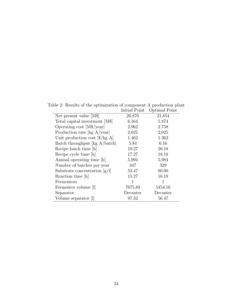
Table 2: Results of the optimization of component A production plantInitial Point Optimal Point
Net present value [M$] 20,870 21,854Total capital investment [M$] 6.164 5.874Operating cost [M$/year] 2.962 2.758Production rate [kg A/year] 2,025 2,025Unit production cost [$/kg A] 1.462 1.362Batch throughput [kg A/batch] 5.84 6.16Recipe batch time [h] 19.27 20.18Recipe cycle time [h] 17.27 18.18Annual operating time [h] 5,994 5,984Number of batches per year 347 329Substrate concentration [g/l] 53.47 80.00Reaction time [h] 15.27 16.18Fermentors 1 1Fermentor volume [l] 7675.89 5454.16Separator Decanter DecanterVolume separator [l] 97.32 56.47
34

Table 3: Progress of iterations of MIDO algorithm in the optimization of L-lysine productionplantIteration Number NLP1 MILP1 NLP2 MILP2 NLP3 MILP3 NLP4Discrete decisionsFermentors 1 2 2 2 2 3 3Equipment separation phase MF MF MF RVF RVF RVF RVFObjective functionJk [$] 7.01·107 2.00·108 1.66·108 1.85·108 1.95·108 2.26·108 1.82·108CPU time [s] 55.34 0.21 44.04 0.17 41.20 0.19 53.75
35

Table 4: Results of the optimization of L-lysine production plantBase Case Initial Point Optimal Point
Net present value [M$] 172,003 59,276 195,688Total capital investment [M$] 101.766 55.369 79.885Operating cost [M$/year] 10.631 4.854 8.830Production rate [tones L-lysine/year] 6,202 2,611 6,202Unit Production cost [$/kg L-lysine] 1.71 1.86 1.42Batch Throughput [tons L-lysine/batch] 29.674 27.783 44.300Recipe Batch time [h] 111.07 110.46 137.67Recipe Cycle time [h] 37.51 83.51 55.81Number of batches per year 209 94 140Concentration Threonine [g/l] 1.62 1.62 1.92Concentration Glucose [g/l] 48.72 48.72 94.61Initial Volume Ferment [m3] 310.34 310.34 282.77Reaction time [h] 71.01 71.01 97.16Fermentors 3 1 2Space-time yield [g/l·h] 1.022 1.022 1.103Overall yield [g/g] 0.299 0.299 0.316Separator RVF MF RVF
36

List of Figures
1 Flowchart of the proposed algorithm . . . . . . . . . . . . . . . . . . . . . . 38
2 Main steps in the resolution of the NLP sub-problem . . . . . . . . . . . . . 39
3 Process flow diagram of a typical ferementation process . . . . . . . . . . . . 40
4 Preliminary analysis of the decision variables in the case study 1 . . . . . . . 41
5 Completed reaction time (i.e., reaction time for which concentration of sub-
strate is zero)versus substrate concentration . . . . . . . . . . . . . . . . . . 42
6 L-lysine production plant (adapted from Heinzle et al.,2006) . . . . . . . . . 43
7 Preliminary analysis of the decision variables in case study 2 . . . . . . . . . 44
8 Preliminary analysis of the decision variables in case study 2 . . . . . . . . . 45
37

Figure 1: Flowchart of the proposed algorithm
38

Figure 2: Main steps in the resolution of the NLP sub-problem
39

Figure 3: Process flow diagram of a typical ferementation process
40

5 10 15 20 250
0.5
1
1.5
2
Reaction Time [h]
Con
cent
ratio
n of
A a
fter
reac
tion
[g/l]
Num
ber
batc
hes
per
year
Csin
= 80g/L
Csin
= 50g/L
Csin
= 30g/L
NºBatches 0
500
1000
1500
2000
(a) Concentration of A and number of batches versus reaction time for afixed demand of 2025 kg/yr
30 40 50 60 70 800
1
2
0.5
1.5
Substrate concentration [g/l]
Con
cent
ratio
n A
afte
r re
actio
n [g
/l]
Num
ber
of b
atch
es p
er y
ear
Cs Reac Time = 25hCs Reac Time = 20hCs Reac Time = 15hNº Batches Reac Time = 25hNº Batches Reac Time = 20hNº Batches Reac Time = 15h
700
600
800
400
500
(b) Concentration of A and number of batches versus initial substrateconcentration for a fixed demand of 2025 kg/yr
Figure 4: Preliminary analysis of the decision variables in the case study 1
41

0 10 20 30 40 50 60 70 800
2
4
6
8
10
12
14
16
18
Substrate Concentration [g/l]
Com
plet
ed R
eact
ion
Tim
e [h
]
Figure 5: Completed reaction time (i.e., reaction time for which concentration of substrateis zero)versus substrate concentration
42

Figure 6: L-lysine production plant (adapted from Heinzle et al.,2006)
43

0.6 0.8 1 1.2 1.4 1.6 1.8 21.6
1.65
1.7
1.75
1.8
1.85
1.9
1.95
2
Initial threonine concentration [g/L]
Uni
t pro
duct
ion
cost
[$/k
g]
Spa
ce−
time
yiel
d (S
TY
) [g
/l·h]
& O
vera
ll yi
eld
(Yoa
) [g
/g]
Unit CostSTYYoa
0
0.15
0.30
0.45
0.60
1.20
1.05
0.90
0.75
(a) Relationship between the unit production cost, STY and Yoa and theinitial threonine concentration (CThr), maintaining the rest of the decisionvariables constant
40 50 60 70 80 90 1001.6
1.65
1.7
1.75
1.8
1.85
1.9
1.95
2
Initial glucose concentration [g/L]
Uni
t pro
duct
ion
cost
[$/k
g]
Spa
ce−
time
yiel
d (S
TY
) [g
/l·h]
&O
vera
ll yi
eld
(Yoa
) [g
/g]
Unit CostSTYYoa
0.30
0
0.15
0.45
0.60
0.75
0.90
1.05
1.20
(b) Relationship between the unit production cost, STY and Yoa and theinitial glucose concentration (Csin), maintaining the rest of the decisionvariables constant
Figure 7: Preliminary analysis of the decision variables in case study 2
44

240 260 280 300 320 340 360 380 4001.6
1.65
1.7
1.75
1.8
1.85
1.9
1.95
2
Initial reaction volume [m3]
Uni
t pro
duct
ion
cost
[$/k
g]
Spa
ce−
time
yiel
d (S
TY
) [g
/L h
] &O
vera
ll yi
eld
(Yoa
) [g
/g]
Unit CostSTYYoa
0
0.75
0.90
1.05
1.20
0.30
0.15
0
0.45
0.60
(a) Relationship between the unit production cost, STY and Yoa andthe initial reactor volume, maintaining the rest of the decision variablesconstant
40 50 60 70 80 90 1001
1.5
2
2.5
3
3.5
4
Reaction time [h]
Uni
t pro
duct
ion
cost
[$/k
g]
Spa
ce−
time
yiel
d (S
TY
) [g
/l·h]
&O
vera
ll yi
eld
(Yoa
) [g
/g]
Unit CostSTYYoa
0
0.20
0.40
0.80
1.00
1.20
0.60
(b) Relationship between the unit production cost, STY and Yoa and theinitial reaction time, maintaining the rest of the decision variables constant
Figure 8: Preliminary analysis of the decision variables in case study 2
45