a global terrestrial monitoring network integrating tower fluxes

A Global Terrestrial Monitoring NetworkIntegrating Tower Fluxes, Flask Sampling,Ecosystem Modeling and EOS Satellite Data

S. W. Running,* D. D. Baldocchi,† D. P. Turner,‡ S. T. Gower,§P. S. Bakwin,‖ and K. A. Hibbard¶

Accurate monitoring of global scale changes in the ter- OVERVIEW OF GLOBAL TERRESTRIALMONITORING AND VALIDATIONrestrial biosphere has become acutely important as the

scope of human impacts on biological systems and atmo- The dynamics of the terrestrial biosphere are an integralspheric chemistry grows. For example, the Kyoto Proto- part of global change. Society needs to know particularlycol of 1997 signals some of the dramatic socioeconomic if the “human habitability” of the biosphere is decreas-and political decisions that may lie ahead concerning ing, especially because more humans are inhabiting theCO2 emissions and global carbon cycle impacts. These land each year. One direct way of quantifying humandecisions will rely heavily on accurate measures of global habitability is by evaluation of the vegetation cover andbiospheric changes (Schimel, 1998; IGBP TCWG, 1998). the primary productivity that provides food, fiber, andAn array of national and international programs have in- fuel for human endeavors. The distribution, health, andaugurated global satellite observations, critical field mea- productivity of global vegetation is typically evaluated insurements of carbon and water fluxes, and global model the context of the global carbon budget. Much of whatdevelopment for the purposes of beginning to monitor the is known about the contemporary global carbon budgetbiosphere. The detection by these programs of interan- has been learned from careful observations of atmo-nual variability of ecosystem fluxes and of longer term spheric CO2 concentration trends and 13C/12C isotope ra-trends will permit early indication of fundamental bi- tios (d13C), interpreted with global circulation models.ospheric changes which might otherwise go undetected From these studies we have learned the following impor-until major biome conversion begins. This article de- tant things about the global carbon cycle:scribes a blueprint for more comprehensive coordination

1. On average over the last 40 years roughly half ofof the various flux measurement and modeling activitiesthe annual anthropogenic input of CO2 to the at-into a global terrestrial monitoring network that willmosphere is taken up by the oceans and the ter-have direct relevance to the political decision making ofrestrial biosphere (Keeling et al., 1989).global change. Elsevier Science Inc., 1999

2. Interpretation of the latitudinal gradient of atmo-spheric CO2, using transport models indicates thata significant portion of the net uptake of CO2 oc-

* Numerical Terradynamic Simulation Group, School of Forestry, curs at midlatitudes of the Northern HemisphereUniversity of Montana, Missoula(Tans et al., 1990; Ciais et al., 1995; Denning et† ATDD, Oak Ridge National Laboratory, Oak Ridge, Tennessee

‡ Forest Science Department, Oregon State University, Corvallis al., 1995).§ Department of Forestry, University of Wisconsin, Madison 3. There are large year-to-year changes in the net‖ NOAA/CMDL, Boulder, Colorado

uptake of CO2 by the terrestrial biosphere. These¶ Climate Change Research Center, University of New Hamp-shire, Durham changes are associated with climate anomalies

Address correspondence to S. W. Running, Numerical Terrady- such as ENSO (Conway et al., 1994; Keeling etnamic Simulation Group, School of Forestry, University of Montana, al., 1995; Keeling et al., 1996).Missoula, MT 59812. E-mail: [email protected]

Received 10 August 1998; revised 15 April 1999. 4. The seasonality of terrestrial biosphere carbon

REMOTE SENS. ENVIRON. 70:108–127 (1999)Elsevier Science Inc., 1999 0034-4257/99/$–see front matter655 Avenue of the Americas, New York, NY 10010 PII S0034-4257(99)00061-9

Global Terrestrial Monitoring Network 109

flux appears to be changing as indicated by shifts tions already exists. The current eddy flux network ofsites is growing rapidly and becoming increasingly orga-in the timing and amplitude of the seasonal cycle

of atmospheric CO2 measured at many “back- nized. Third, the flux towers provide a critical infrastruc-ture of organized personnel and equipment for otherground” sites. In particular, it appears that spring

is beginning earlier and fall arriving later (Ran- comprehensive measurements, including ecophysiology,structure and biomass of the vegetation, fluxes of otherderson et al., 1997; Field et al., 1998). This resultgreenhouse gases, and micrometeorology.is supported by satellite phenology observations

Monitoring of the spatial and temporal patterns in(Myneni et al., 1997a).the concentration of CO2, O2, and their isotopic variantsThese indications of biospheric changes point to thecan provide the basis for estimates of carbon cycle fluxesneed to 1) better understand and monitor the processesat large scales (Tans et al., 1996). The remarkablethat regulate uptake and release of CO2 by terrestrialachievements from the geochemistry approach, begin-ecosystems, 2) provide verification from more directning with the observations at Mona Loa, which first de-ground-based measurements, and 3) employ satellite ob-tected the upward trend in the global atmospheric CO2servations to clarify spatial patterns in ecosystem func-concentration, establish its importance for biospheric

tion. There is also new interest in computing sources and monitoring. The limitations in the geochemistry ap-sinks of carbon for individual nations that will challenge proach for terrestrial monitoring are that it is not spa-current data availability. This article suggests how a num- tially explicit, and generally indicates the net effect ofber of current international research activities can be in- multiple, potentially opposing, processes.tegrated into a biospheric monitoring program that effi-

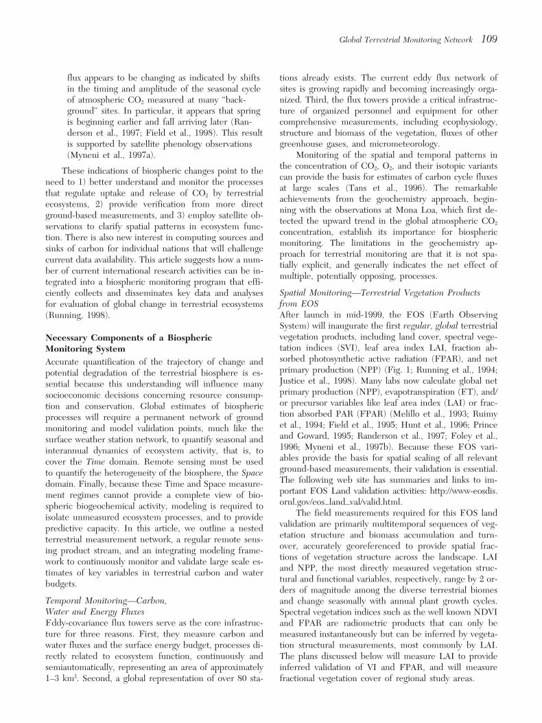
Spatial Monitoring—Terrestrial Vegetation Productsciently collects and disseminates key data and analysesfrom EOSfor evaluation of global change in terrestrial ecosystemsAfter launch in mid-1999, the EOS (Earth Observing(Running, 1998).System) will inaugurate the first regular, global terrestrialvegetation products, including land cover, spectral vege-Necessary Components of a Biospherictation indices (SVI), leaf area index LAI, fraction ab-Monitoring Systemsorbed photosynthetic active radiation (FPAR), and netAccurate quantification of the trajectory of change andprimary production (NPP) (Fig. 1; Running et al., 1994;potential degradation of the terrestrial biosphere is es-Justice et al., 1998). Many labs now calculate global netsential because this understanding will influence manyprimary production (NPP), evapotranspiration (ET), and/socioeconomic decisions concerning resource consump-or precursor variables like leaf area index (LAI) or frac-tion and conservation. Global estimates of biospheriction absorbed PAR (FPAR) (Melillo et al., 1993; Ruimyprocesses will require a permanent network of groundet al., 1994; Field et al., 1995; Hunt et al., 1996; Princemonitoring and model validation points, much like theand Goward, 1995; Randerson et al., 1997; Foley et al.,surface weather station network, to quantify seasonal and1996; Myneni et al., 1997b). Because these EOS vari-interannual dynamics of ecosystem activity, that is, toables provide the basis for spatial scaling of all relevantcover the Time domain. Remote sensing must be usedground-based measurements, their validation is essential.to quantify the heterogeneity of the biosphere, the SpaceThe following web site has summaries and links to im-domain. Finally, because these Time and Space measure-portant EOS Land validation activities: http://www-eosdis.ment regimes cannot provide a complete view of bio-ornl.gov/eos land val/valid.html.spheric biogeochemical activity, modeling is required to

The field measurements required for this EOS landisolate unmeasured ecosystem processes, and to providevalidation are primarily multitemporal sequences of veg-predictive capacity. In this article, we outline a nestedetation structure and biomass accumulation and turn-terrestrial measurement network, a regular remote sens-over, accurately georeferenced to provide spatial frac-ing product stream, and an integrating modeling frame-tions of vegetation structure across the landscape. LAIwork to continuously monitor and validate large scale es-and NPP, the most directly measured vegetation struc-timates of key variables in terrestrial carbon and watertural and functional variables, respectively, range by 2 or-budgets.ders of magnitude among the diverse terrestrial biomes

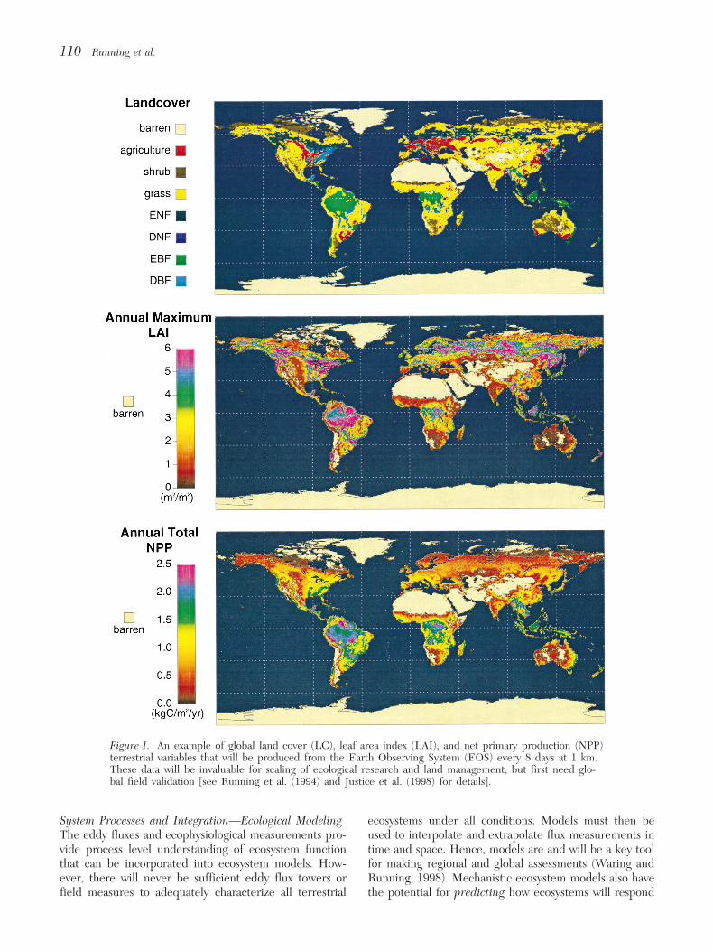
Temporal Monitoring—Carbon, and change seasonally with annual plant growth cycles.Water and Energy Fluxes Spectral vegetation indices such as the well known NDVIEddy-covariance flux towers serve as the core infrastruc- and FPAR are radiometric products that can only beture for three reasons. First, they measure carbon and measured instantaneously but can be inferred by vegeta-

tion structural measurements, most commonly by LAI.water fluxes and the surface energy budget, processes di-rectly related to ecosystem function, continuously and The plans discussed below will measure LAI to provide

inferred validation of VI and FPAR, and will measuresemiautomatically, representing an area of approximately1–3 km2. Second, a global representation of over 80 sta- fractional vegetation cover of regional study areas.

110 Running et al.

Figure 1. An example of global land cover (LC), leaf area index (LAI), and net primary production (NPP)terrestrial variables that will be produced from the Earth Observing System (EOS) every 8 days at 1 km.These data will be invaluable for scaling of ecological research and land management, but first need glo-bal field validation [see Running et al. (1994) and Justice et al. (1998) for details].

System Processes and Integration—Ecological Modeling ecosystems under all conditions. Models must then beused to interpolate and extrapolate flux measurements inThe eddy fluxes and ecophysiological measurements pro-

vide process level understanding of ecosystem function time and space. Hence, models are and will be a key toolfor making regional and global assessments (Waring andthat can be incorporated into ecosystem models. How-

ever, there will never be sufficient eddy flux towers or Running, 1998). Mechanistic ecosystem models also havethe potential for predicting how ecosystems will respondfield measures to adequately characterize all terrestrial


to future changes in atmospheric CO2, temperature, land when soil moisture changes and groundwater losses areignored. Also, both of these historical ecosystem mea-use change, nitrogen loading, and precipitation.sures, NPP and Q, are typically measured on a weekly-to-monthly basis, so are temporally inconsistent with theCritical Variables in a Global Terrestrial

Monitoring System continuous flux tower measures of NEE and ET. Addi-tionally, there are spatial scale mismatches. The towerWe initially focus on one key variable each of the carbonfluxes represent a footprint of roughly 1–3 km2, whileand water cycles: net primary production (NPP) andNPP is typically measured on .0.1 ha plot, and water-evapotranspiration (ET). The carbon budget consists ofsheds can drain many hundreds of square kilometers.several major processes that describe the exchange ofProcess-based terrestrial ecosystem models, driven bycarbon dioxide between terrestrial ecosystems and the at-spatially represented climate and satellite derived vegeta-mosphere. Gross primary production (GPP) is the totaltion parameters, are essential for integrating the suite ofcarbon assimilated by vegetation. A fraction of GPP isfield-based measurements of inconsistent temporal andlost back to the atmosphere as the result of autotrophicspatial scale to provide a complete and consistent viewrespiration (RA). Net primary production (NPP), the bal-of global biospheric function.ance between GPP and autotrophic respiration, is allo-

We now visit each of four components critical to acated to wood, foliage, roots, reproductive tissues, stor-comprehensive monitoring scheme and identify associ-age, etc. NPP, the direct measure of vegetationated on-going research activities. In the temporal dimen-productivity, has been measured from field biomass sur-sion, it is a global flux tower network and a global flaskveys for decades and has the largest historical database.sampling network that are essential. For the spatial di-NPP relates directly to forest, range, and crop productiv-mension, we discuss the EOS products. SVAT modelingity, and so also has high socioeconomic value. NEE, theis then examined as a means of scaling carbon and waternet exchange of CO2 between terrestrial ecosystems andflux over space and time. Subsequently, we consider thethe atmosphere, is measured by flux towers. NEE hasnature of the required information flow among thesehigh scientific relevance for terrestrial carbon budgetscomponents and identify international programs con-and greenhouse gas production, but less direct socioeco-cerned with integration.nomic significance.

Under optimal conditions, NEE is measured contin-uously and calculated on a half-hourly or hourly basis, GLOBAL FLUX TOWER NETWORK (FLUXNET)whereas the field-based NPP is measured periodically

The cornerstone of this global terrestrial vegetation mon-and calculated on an annual basis. The two fluxes areitoring is the tower flux network, FLUXNET. This globalrelated in that if NEE is summed over a year, the sumarray of tower sites is currently comprised of regionalshould be the difference between NPP and heterotro-networks in Europe (EUROFLUX), North Americaphic respiration (RH) summed over the year. Thus(AmeriFlux), Asia (JapanNet, OzFlux), and Latin Amer-NEEannual5NPPannual2RH annual . (1)ica (LBA). The towers provide a continuous and repre-

Note that on a daily time step NEE is related to sentative measure of terrestrial carbon cycle dynamics,GPP and RA in Eq. (2): and an important ancillary suite of measurements of en-

ergy and water fluxes for interpreting carbon fluxes (Fig.NEEdaily5GPPdaily2(RH1RA)daily . (2)2). The role of FLUXNET includes coordinating the re-

NPP and NEE are related theoretically, but the two gional networks so that information can be attained at acarbon fluxes are measured at very different temporal global scale, ensuring site to site intercomparability, co-and spatial scales, necessitating an integrated approach ordinating enhancements to current network plans andto provide global coverage for rapid validation and moni- operation of a global archive and distribution center attoring opportunities. The ultimate goal is to validate the Oak Ridge DAAC. The FLUXNET project web ad-global measures of NEE and NPP. dress is http://daacl.ESD.ORNL.Gov/FLUXNET/. The

The other primary variable, evapotranspiration (ET), web sites contain measurement protocols for consistency,is a component of the surface hydrologic balance and an and data on site, vegetation, climate, and soil characteris-integral part of surface energy partitioning. ET is also tics. It provides a route for users to gain access of hourlymeasured continuously by a flux tower, providing a high meteorological and flux measurements and proper docu-temporal resolution measurement of the partitioning of mentation.precipitation (PPT) in the hydrological budget of an eco- The FLUXNET concept originated at a workshop onsystem. However, much like with NPP and NEP, the “Strategies for Long Term Studies of CO2 and Water Va-variable of the hydrologic cycle with the longest history por Fluxes over Terrestrial Ecosystems” held in Marchand widest distributed data is watershed discharge Q. 1995 in La Thuile, Italy (Baldocchi et al., 1996). The firstThese variables are generally related as in Eq. (3): organized flux tower network was EUROFLUX, which

now involves long-term flux measurements of carbon di-Q5PPT2ET (3)

112 Running et al.

Figure 2. A generalized FLUXNET tower configuration diagram, showing instrument deployment and key carbon and waterfluxes measured. Atmospheric optical measurements, automated surface spectral measurements, physiological process studies,flask sampling, and stable isotope sampling are all additions that can be accommodated into this framework to provide a moreversatile monitoring system.

oxide and water vapor over 15 forest sites in the United entering and leaving the vegetation. Vertical flux densi-Kingdom, France, Italy, Belgium, Germany, Sweden, ties of CO2 and water vapor between the biosphere andFinland, Denmark, The Netherlands, and Iceland. A the atmosphere are proportional to the mean covariancewebsite is located at http://www.unitus.it/eflux/euro.html. between vertical velocity and scalar fluctuations. This de-In 1996, AmeriFlux was formed under the aegis of the pendency requires the implementation of sensitive, accu-DOE, NIGEC program, with additional support by rate, and fast-responding anemometry, hygrometery,NASA, and NOAA. The website is http://www.esd.ornl. thermometry, and infrared spectrometry to measure thegov/programs/NIGEC. vertical and horizontal wind velocity, humidity, tempera-

ture, and CO2 concentration.Eddy Covariance Principles Errors arise from atmospheric, surface, and instru-

mental origins, and they may be random, fully systematicThe eddy covariance method is a well-developed methodand/or selective (Goulden et al., 1996). Most random er-for measuring trace gas flux densities between the bio-rors are associated with violations of atmospheric stationar-sphere and atmosphere (Baldocchi et al., 1988; Len-ity and the consequences of intermittent turbulence. In-schow, 1995; Moncrieff et al., 1996). This method is de-strument errors are systematic, caused by insufficientrived from the conservation of mass and is most applica-time response of a sensor, the spatial separation betweenble for steady-state conditions over flat terrain with ana sensor and an anemometer, digital filtering of the timeextended tract of uniform vegetation. If these conditionssignal, aerodynamic flow distortion, calibration drift, lossare met, eddy covariance measurements made from aof frequency via sampling over a finite space, and sensortower can be considered to be within the constant fluxnoise (Moore, 1986; Moncrieff et al., 1996). The Ameri-layer, and flux density measured several meters over the

vegetation canopy is equal to the net amount of material Flux, Euroflux, and FLUXNET programs are attempting


to identify and minimize instrumental errors by circulat- over intensive agricultural areas. Future planning shouldidentify the climate/biome combinations of highest prior-ing a set of reference instruments, to which all sites can

be compared. Daily-averaged fluxes reduce the sampling ity to improve global representativeness.errors associated with fluxes measured over 30–60 minintervals. Hence, daily integrals of net carbon flux can be

THE ATMOSPHERIC CO2 FLASK NETWORKaccepted with a reasonable degree of confidence. Goul-den et al. (1996) conclude that the long term precision Inverse Modeling of Carbon Sources and Sinksof eddy covariance flux measurements is 65–10% and The eddy flux tower studies are designed to aid under-the confidence interval about an annual estimate of net standing of processes that drive NEE at the ecosystemcanopy CO2 exchange is 630 g C m22 y21. level, and for evaluation of ecosystem models used for

regional and global integration. However, a top-down ap-Implementation and Operation proach is also needed to test and validate the results ofA typical cost for purchasing instruments to make core the model extrapolations to global and regional scales.measurements is on the order of $40–to $50k (US); this Data from the global CO2 mixing ratio and isotope ratiocost can double if spare sensors, data telemetry, and data measurement network (NOAA/CMDL/Cooperative Airarchiving hardware are purchased. The cost of site infra- Sampling Network, website at http://www.cmdl.noaa.gov/structure is extra and will vary according to the remote- ccg/), when interpreted within general circulation mod-ness of the site (the need for a road and line-power), the els, can provide constraints at least at this scale. The ba-height of the vegetation (whether or not a tall tower sic procedure in this approach is referred to as inversemust be built), and the existence of other facilities. Re- modeling. It involves simulating the global 3-D atmo-cent advances in remote power generation and storage spheric transport using a general circulation model andminimize the need and cost of bringing line power to a tracking the movement and interaction of air parcels hav-remote site. Advances in cellular telephone technology ing different CO2 concentrations. Information on thealso allow access and query of a remote field station from spatial and temporal patterns in measured atmospherichome or the office. The requirement for on-site person- CO2 concentrations derived from flask samples is incor-nel is diminishing, as flux systems become more reliable porated such that sources and sinks of carbon from theand automated. At minimum, a team of two individuals Earth’s surface can be inferred.are required to operate a flux system, and handle the Initially, flask sampling was primarily in well-mixedday-to-day chores of calibration, instrument and com- marine areas. Expansion of the monitoring networks overputer maintenance, data archiving, and periodic site the last decade has improved the spatial resolution withcharacterization (e.g., soil moisture and leaf area mea- which annual fluxes can be determined, so that currentlysurements). fluxes are being estimated at continental scales (Fan et

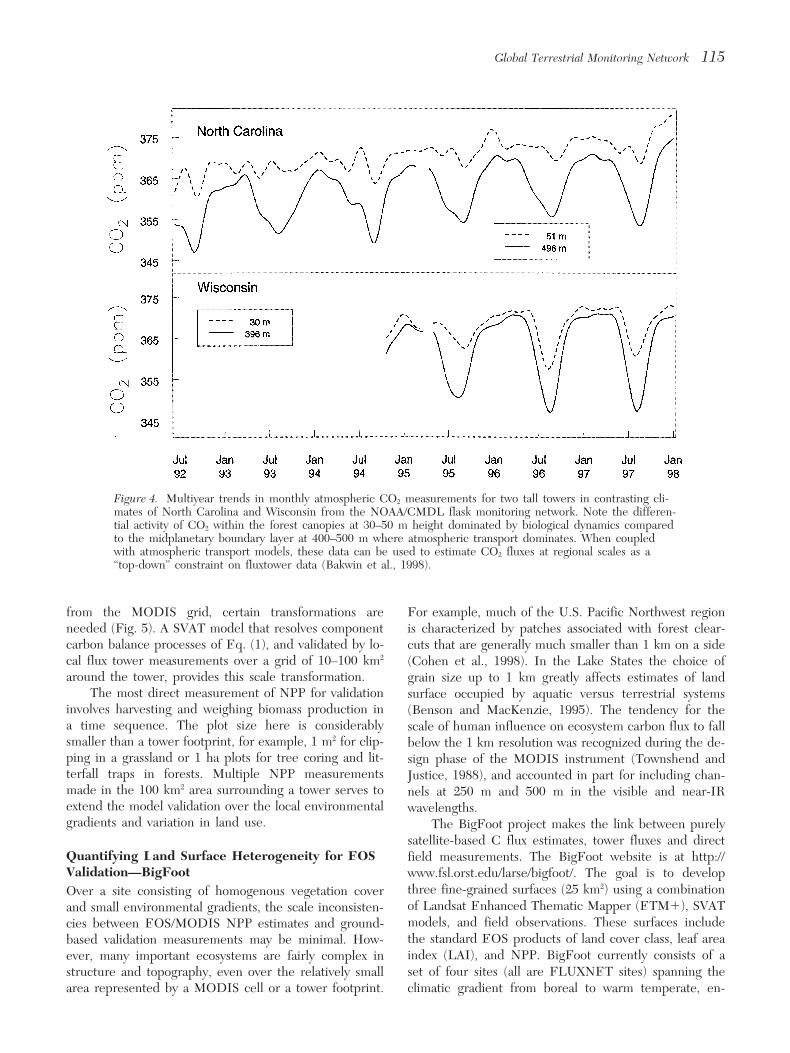
Sites in an organized global flux network can also ex- al., 1998). Sampling at continental sites reveals regionalpect to attract additional activities. A synergism between contrasts in seasonality of flux dynamics, and sampling atflux and meteorological measurements and an array of various heights on tall towers (500 m) identifies gradientsother terrestrial science projects is likely. Terrestrial bio- of CO2 in the boundary layer dynamics (Fig. 4; Bakwinclimatology, remote sensing, atmospheric optical charac- et al., 1998). As sampling density is increased, it will beterization, water resource, and nutritional biogeochemis- possible to use higher resolution transport models, suchtry studies are examples of science that are being as mesoscale models, to deduce surface fluxes at finer

spatial scales. Additional work is needed to develop andattracted to the flux network sites (Fig. 2).refine the transport models, and particular attention isrequired to develop parametrizations for simulation ofClimate and Biome Distribution Requirementsthe dynamics of the planetary boundary layer. It is im-Ideally, global terrestrial monitoring/validation sites shouldportant that the resulting estimates of NEE are entirelyencompass the complete range of climate and biome typeindependent of the flux tower measurements, and nearlycombinations. The current global array of flux towers isindependent of the satellite data (satellite data defineshown in Figure 3, mapped over the annual tempera-surface parameters used in the transport models).ture/precipitation climate space of current global vegeta-

tion (Churkina and Running, 1998). It is clear that largeIsotopic Samplingregions, including several important biomes, remain un-

derrepresented including hot desert and cold tundras, The state of development of isotopic measurements (par-ticularly in combination with CO2 flux tower measure-which is inevitable with an ad hoc volunteer global net-

work (Table 1). Also, the correspondence between flux ments), for better understanding the carbon cycle on local,regional, and global scales, was the topic of a workshoptower locations and permanent ecological field sites is

low, illustrating the key role for modeling to spatially ex- titled Biosphere–Atmosphere Stable Isotope Network(BASIN, Snowbird, Utah, 7–10 December 1997). A sum-trapolate results amongst sites. More sites are needed

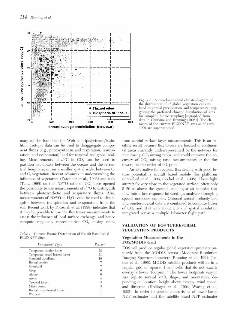
114 Running et al.

Figure 3. A two-dimensional climate diagram ofthe distribution of 18 global vegetation cells re-lated to annual precipitation and temperature, sug-gesting the preferred climatic distribution of sitesfor complete biome sampling [regraphed fromdata in Churkina and Running (1998)]. The cli-mates of the current FLUXNET sites as of early1999 are superimposed.

mary can be found on the Web at http://gcte.org/basin. from careful surface layer measurements. This is an ex-html. Isotopic data can be used to disaggregate compo- citing result because flux towers are located in continen-nent fluxes (e.g., photosynthesis and respiration, transpi- tal areas currently underrepresented by the network forration, and evaporation), and for regional and global scal- monitoring CO2 mixing ratios, and could improve the ac-ing. Measurements of d13C in CO2 can be used to curacy of CO2 mixing ratio measurements at the fluxpartition net uptake between the oceans and the terres- towers on the order of 0.2 ppm.trial biosphere, or, on a smaller spatial scale, between C3 An alternative for regional flux scaling with good fu-and C4 vegetation. Recent advances in understanding the ture potential is aircraft based mobile flux platformsinfluence of vegetation (Farquhar et al., 1993) and soils (Crawford et al., 1996; Oechel et al., 1998). These light(Tans, 1998) on the 18O/16O ratio of CO2 have opened aircraft fly very close to the vegetated surface, often onlythe possibility to use measurements of d18O to distinguish 5–20 m above the ground, and ingest air samples thatbetween photosynthetic and respiratory fluxes. Also, flow into a fast response infrared gas analyzer through ameasurements of 18O/16O in H2O could be used to distin- special nosecone sampler. Onboard aircraft velocity andguish between transpiration and evaporation from the micrometerological data are combined to compute fluxessoil. Recent work by Potosnak et al. (1998) indicates that of CO2 and H20 with about a 3 km2 spatial resolutionit may be possible to use the flux tower measurements to integrated across a multiple kilometer flight path.assess the influence of local surface exchange, and hencecompute regionally representative CO2 mixing ratios

VALIDATION OF EOS TERRESTRIALVEGETATION PRODUCTS

Table 1. Current Biome Distribution of the 80 EstablishedVegetation Measurements in theFLUXNET SitesEOS/MODIS GridFunctional Type PercentEOS will produce regular global vegetation products pri-

Temperate conifer forest 22marily from the MODIS sensor (Moderate ResolutionTemperate broad-leaved forest 21Imaging Spectroradiometer) (Running et al., 1994; Jus-Semiarid woodland 16

Boreal conifer 7 tice et al., 1998). MODIS satellite products will be in aGrassland 7 regular grid of square, 1 km2 cells that do not exactlyCrop 6 overlay a tower “footprint.” The tower footprints vary inAlpine 6

size (up to several km2), shape, and orientation, de-Arctic 4pending on location, height above canopy, wind speed,Tropical forest 3

Mixed forest 3 and direction (Hollinger et al., 1994; Waring et al.,Boreal broad-leaved forest 1 1995). In order to permit comparisons of tower-basedWetland 1 NEE estimates and the satellite-based NPP estimates


Figure 4. Multiyear trends in monthly atmospheric CO2 measurements for two tall towers in contrasting cli-mates of North Carolina and Wisconsin from the NOAA/CMDL flask monitoring network. Note the differen-tial activity of CO2 within the forest canopies at 30–50 m height dominated by biological dynamics comparedto the midplanetary boundary layer at 400–500 m where atmospheric transport dominates. When coupledwith atmospheric transport models, these data can be used to estimate CO2 fluxes at regional scales as a“top-down” constraint on fluxtower data (Bakwin et al., 1998).

from the MODIS grid, certain transformations are For example, much of the U.S. Pacific Northwest regionneeded (Fig. 5). A SVAT model that resolves component is characterized by patches associated with forest clear-carbon balance processes of Eq. (1), and validated by lo- cuts that are generally much smaller than 1 km on a sidecal flux tower measurements over a grid of 10–100 km2 (Cohen et al., 1998). In the Lake States the choice ofaround the tower, provides this scale transformation. grain size up to 1 km greatly affects estimates of land

The most direct measurement of NPP for validation surface occupied by aquatic versus terrestrial systemsinvolves harvesting and weighing biomass production in (Benson and MacKenzie, 1995). The tendency for thea time sequence. The plot size here is considerably scale of human influence on ecosystem carbon flux to fallsmaller than a tower footprint, for example, 1 m2 for clip- below the 1 km resolution was recognized during the de-ping in a grassland or 1 ha plots for tree coring and lit- sign phase of the MODIS instrument (Townshend andterfall traps in forests. Multiple NPP measurements Justice, 1988), and accounted in part for including chan-made in the 100 km2 area surrounding a tower serves to nels at 250 m and 500 m in the visible and near-IRextend the model validation over the local environmental wavelengths.gradients and variation in land use. The BigFoot project makes the link between purely

satellite-based C flux estimates, tower fluxes and directQuantifying Land Surface Heterogeneity for EOS field measurements. The BigFoot website is at http://Validation—BigFoot www.fsl.orst.edu/larse/bigfoot/. The goal is to develop

three fine-grained surfaces (25 km2) using a combinationOver a site consisting of homogenous vegetation coverof Landsat Enhanced Thematic Mapper (ETM1), SVATand small environmental gradients, the scale inconsisten-models, and field observations. These surfaces includecies between EOS/MODIS NPP estimates and ground-the standard EOS products of land cover class, leaf areabased validation measurements may be minimal. How-index (LAI), and NPP. BigFoot currently consists of aever, many important ecosystems are fairly complex inset of four sites (all are FLUXNET sites) spanning thestructure and topography, even over the relatively small

area represented by a MODIS cell or a tower footprint. climatic gradient from boreal to warm temperate, en-

116 Running et al.

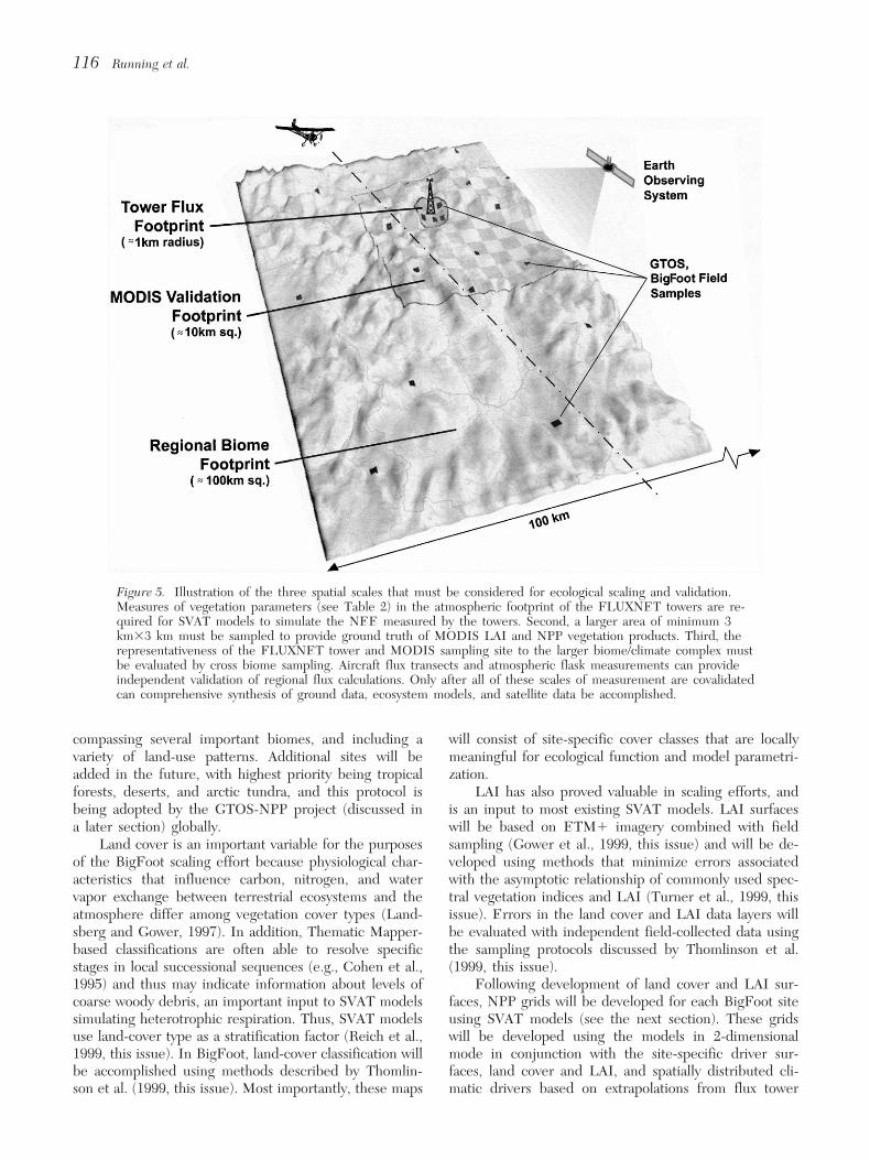
Figure 5. Illustration of the three spatial scales that must be considered for ecological scaling and validation.Measures of vegetation parameters (see Table 2) in the atmospheric footprint of the FLUXNET towers are re-quired for SVAT models to simulate the NEE measured by the towers. Second, a larger area of minimum 3km33 km must be sampled to provide ground truth of MODIS LAI and NPP vegetation products. Third, therepresentativeness of the FLUXNET tower and MODIS sampling site to the larger biome/climate complex mustbe evaluated by cross biome sampling. Aircraft flux transects and atmospheric flask measurements can provideindependent validation of regional flux calculations. Only after all of these scales of measurement are covalidatedcan comprehensive synthesis of ground data, ecosystem models, and satellite data be accomplished.

compassing several important biomes, and including a will consist of site-specific cover classes that are locallymeaningful for ecological function and model parametri-variety of land-use patterns. Additional sites will be

added in the future, with highest priority being tropical zation.LAI has also proved valuable in scaling efforts, andforests, deserts, and arctic tundra, and this protocol is

being adopted by the GTOS-NPP project (discussed in is an input to most existing SVAT models. LAI surfaceswill be based on ETM1 imagery combined with fielda later section) globally.

Land cover is an important variable for the purposes sampling (Gower et al., 1999, this issue) and will be de-veloped using methods that minimize errors associatedof the BigFoot scaling effort because physiological char-

acteristics that influence carbon, nitrogen, and water with the asymptotic relationship of commonly used spec-tral vegetation indices and LAI (Turner et al., 1999, thisvapor exchange between terrestrial ecosystems and the

atmosphere differ among vegetation cover types (Land- issue). Errors in the land cover and LAI data layers willbe evaluated with independent field-collected data usingsberg and Gower, 1997). In addition, Thematic Mapper-

based classifications are often able to resolve specific the sampling protocols discussed by Thomlinson et al.(1999, this issue).stages in local successional sequences (e.g., Cohen et al.,

1995) and thus may indicate information about levels of Following development of land cover and LAI sur-faces, NPP grids will be developed for each BigFoot sitecoarse woody debris, an important input to SVAT models

simulating heterotrophic respiration. Thus, SVAT models using SVAT models (see the next section). These gridswill be developed using the models in 2-dimensionaluse land-cover type as a stratification factor (Reich et al.,

1999, this issue). In BigFoot, land-cover classification will mode in conjunction with the site-specific driver sur-faces, land cover and LAI, and spatially distributed cli-be accomplished using methods described by Thomlin-

son et al. (1999, this issue). Most importantly, these maps matic drivers based on extrapolations from flux tower


meteorological observations. Beside the daily time step SVAT Model Requirements for 1-D Flux Modelingvalidation of GPP and ET at BigFoot sites with flux SVAT models have been designed with a wide array oftowers, the BigFoot NPP surfaces will be carefully evalu- system complexities (Fig. 6). For example, some modelsated for error by reference to a gridded network of define each age class and branch whorl of leaves, whileground measurements of NPP, collected according to others use only simple LAI. Time resolutions of variousmethods described by Gower et al. (1999, this issue). As- models range from 1 h to monthly. The land surfacesuming the errors in these NPP surfaces are acceptable, models such as BATS and SiB in GCMs are effectivelythe fine-grained gridded surface over a 25 km2 area can SVAT models despite being used at very coarse spatialthen be directly compared to NPP estimates derived grids (Dickinson, 1995). SVAT models of highest rele-from MODIS data over the same area. If the MODIS- vance to FLUXNET have time resolutions in the hourly–based estimates do not satisfactorily agree with the Big- daily domain, treat canopy structure fairly explicitly, andFoot estimates, it will be critical to identify causal resolve components of the carbon balance (photosynthe-factors. sis, heterotrophic and autotrophic respiration, and al-

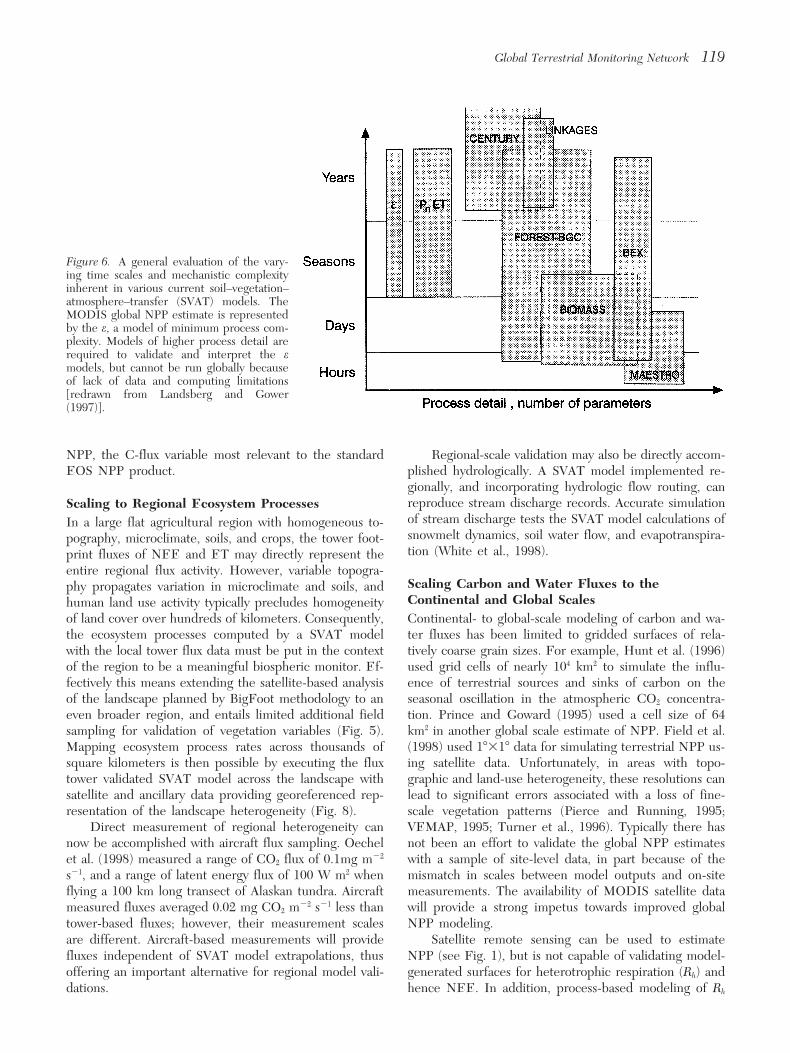
BigFoot will isolate and test three key factors— location). Likewise, stand water balance components,spatial resolution, land cover classification scheme, and (canopy interception, snowpack, soil water storage, evap-light use efficiency factors—that may contribute to dif- oration, and transpiration) must be explicitly computed.ferences between EOS-based and BigFoot NPP esti- All of the leading SVAT models incorporate some treat-mates. To evaluate the role of spatial resolution, the Big- ment of nutrient biogeochemistry interactions with car-Foot 25 m grids for input variables will be aggregated to bon and water processes. However, given these require-resolutions of 250 m, 500 m, and 1000 m using a variety ments, there are still many available and appropriateof standard and experimental algorithms. Model runs will SVAT models [see recent books by Landsberg andthen be made at each spatial resolution and comparisons Gower (1997) and Waring and Running (1998)]. What is

needed for a coordinated global program are some com-of simulated NPP at the different resolutions (includingmon protocols, of variables, units, timesteps, etc. that25 m) will be made with each other and with the EOS/would allow cooperation and intercomparisons amongMODIS 1 km NPP products. Results of these scaling ex-groups using different SVAT models in their space/timeercises over the range of biomes and land use patternsscaling. The 1-D SVAT models require meteorologicalincluded in BigFoot will test both SVAT models and sat-driving variables measured at the tower, the initializingellite-based NPP algorithms.biomass components of the vegetation, and certain soilphysical and chemical properties. All SVAT models have

SYSTEM INTEGRATION AND SCALING somewhat different specific requirements, but the gen-WITH MODELS eral list of inputs found in Table 2 covers most of them.To transform basic tower flux and flask data and global

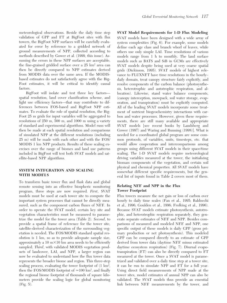
Relating NEE and NPP in the Fluxremote sensing into an effective biospheric monitoringTower Footprintprogram, three steps are now required. First, SVAT

models must be used at each tower site to compute the Flux towers measure the net gain or loss of carbon overhourly to daily time scales (Fan et al., 1995; Baldocchiimportant system processes that cannot be directly mea-

sured, such as the component carbon fluxes of NEE. In et al., 1996; Goulden et al., 1996; Frolking et al., 1996).Because SVAT models estimate photosynthesis, autotro-order to operate the SVAT model, certain key site and

vegetation characteristics must be measured to parame- phic, and heterotrophic respiration separately, they gen-erate separate estimates of NEE and NPP. Besides com-trize the model for the tower area (Table 2). Second, to

provide a spatial frame of reference for the tower site, parisons of measured and modeled NEE and NPP, onespecific output of these models is daily GPP (gross pri-satellite-derived characterization of the surrounding veg-

etation is needed. The EOS/MODIS standard spatial res- mary production or net photosynthesis). This modeledGPP can be compared directly to an estimate of GPPolution is 1 km, so as to provide adequate sample size,

approximately a 10 m310 km area needs to be efficiently derived from tower data (daytime NEE minus estimateddaytime ecosystem respiration) (Fig. 7). Diurnal evapo-sampled. Third, with validated MODIS vegetation prod-

ucts of landcover, LAI, and NPP, a larger region can transpiration (ET) can also be directly compared to ETmeasured at the tower. Once a SVAT model is parame-now be evaluated to understand how the flux tower data

represents the broader biome and region. This three-step trized and validated over a daily time step at a tower site,it can be run to simulate NPP and ET for a full year.scaling process, evaluating the tower footprint of (1 km2,

then the EOS/MODIS footprint of .100 km2, and finally Using direct field measurements of NPP made at thetower sites, model estimates of annual NPP can also bethe regional biome footprint of thousands of square kilo-

meters provide the scaling logic for global monitoring validated. The SVAT models thus provide an essentiallink between NEE measurements by the tower, and(Fig. 5).

118 Running et al.

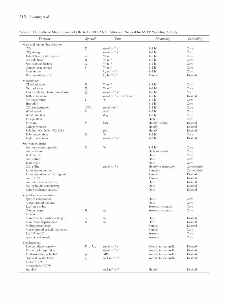
Table 2. The Suite of Measurements Collected at FLUXNET Sites and Needed for SVAT Modeling Activity

Variable Symbol Unit Frequency Criticality

Mass and energy flux densitiesCO2 Fc lmol m22 s21 1–2 h21 CoreCO2 storage lmol m22 s21 1–2 h21 CoreLatent heat (water vapor) kE W m22 1–2 h21 CoreSensible heat H W m22 1–2 h21 CoreSoil heat conduction G W m22 1–2 h21 CoreCanopy heat storage S W m22 1–2 h21 CoreMomentum kg m21 s22 1–2 h21 CoreDry deposition of N kg ha21 y21 Annual Desired

MeteorologyGlobal radiation Rg W m22 1–2 h21 CoreNet radiation Rn W m22 1–2 h21 CorePhotosynthetic photon flux density Qp lmol m22 s21 1–2 h21 CoreDiffuse radiation lmol m22 s21 or W m22 1–2 h21 DesiredAir temperature Ta 8C 1–2 h21 CoreHumidity 1–2 h21 CoreCO2 concentration [CO2] lmol mol21 1–2 h21 CoreWind speed U m s21 1–2 h21 CoreWind direction deg 1–2 h21 CorePrecipitation Daily CorePressure P kPa Hourly to daily DesiredCanopy wetness Hourly DesiredPollution (O3, NO2, NO, SO2) ppb Hourly DesiredBole temperature Tb 8C 1–2 h21 CoreLight transmission lmol m22 s21 1–2 h21 Desired

Soil characteristicsSoil temperature profiles Ts 8C 1–2 h21 CoreSoil moisture Daily to weekly CoreBulk density Once CoreSoil texture Once CoreRoot depth Once CoreCO2 efflux lmol m22 s21 Hourly to seasonally Core/desiredLitter decomposition Annually Core/desiredLitter chemistry (C, N, Lignin) Annual DesiredSoil (C, N) Annual DesiredSoil thermal conductivity Once DesiredSoil hydraulic conductivity Once DesiredCation exchange capacity Once Desired

Vegetation characteristicsSpecies composition Once CoreAbove-ground biomass Once CoreLeaf area index Seasonal to annual CoreCanopy height H m Seasonal to annual CoreAlbedoAerodynamic roughness length z0 m Once DesiredZero plane displacement D m Once DesiredMultispectral image Annual DesiredAbove-ground growth increment Annual CoreLeaf N and C Seasonal CoreSpecific leaf weight Seasonal Core

EcophysiologyPhotosynthetic capacity Vcmax, Jmax lmol m22 s21 Weekly to seasonally DesiredTissue dark respiration lmol m22 s21 Weekly to seasonally DesiredPredawn water potential w MPa Weekly to seasonally DesiredStomatal conductance gs mol m22 s21 Weekly to seasonally DesiredTissue 13C/12CAtmospheric 13C/12CSap flow mol m22 s21 Hourly Desired


Figure 6. A general evaluation of the vary-ing time scales and mechanistic complexityinherent in various current soil–vegetation–atmosphere–transfer (SVAT) models. TheMODIS global NPP estimate is representedby the e, a model of minimum process com-plexity. Models of higher process detail arerequired to validate and interpret the emodels, but cannot be run globally becauseof lack of data and computing limitations[redrawn from Landsberg and Gower(1997)].

NPP, the C-flux variable most relevant to the standard Regional-scale validation may also be directly accom-plished hydrologically. A SVAT model implemented re-EOS NPP product.gionally, and incorporating hydrologic flow routing, canreproduce stream discharge records. Accurate simulationScaling to Regional Ecosystem Processesof stream discharge tests the SVAT model calculations ofIn a large flat agricultural region with homogeneous to-snowmelt dynamics, soil water flow, and evapotranspira-pography, microclimate, soils, and crops, the tower foot-tion (White et al., 1998).print fluxes of NEE and ET may directly represent the

entire regional flux activity. However, variable topogra-Scaling Carbon and Water Fluxes to thephy propagates variation in microclimate and soils, andContinental and Global Scaleshuman land use activity typically precludes homogeneity

of land cover over hundreds of kilometers. Consequently, Continental- to global-scale modeling of carbon and wa-ter fluxes has been limited to gridded surfaces of rela-the ecosystem processes computed by a SVAT model

with the local tower flux data must be put in the context tively coarse grain sizes. For example, Hunt et al. (1996)used grid cells of nearly 104 km2 to simulate the influ-of the region to be a meaningful biospheric monitor. Ef-

fectively this means extending the satellite-based analysis ence of terrestrial sources and sinks of carbon on theseasonal oscillation in the atmospheric CO2 concentra-of the landscape planned by BigFoot methodology to an

even broader region, and entails limited additional field tion. Prince and Goward (1995) used a cell size of 64km2 in another global scale estimate of NPP. Field et al.sampling for validation of vegetation variables (Fig. 5).

Mapping ecosystem process rates across thousands of (1998) used 18318 data for simulating terrestrial NPP us-ing satellite data. Unfortunately, in areas with topo-square kilometers is then possible by executing the flux

tower validated SVAT model across the landscape with graphic and land-use heterogeneity, these resolutions canlead to significant errors associated with a loss of fine-satellite and ancillary data providing georeferenced rep-

resentation of the landscape heterogeneity (Fig. 8). scale vegetation patterns (Pierce and Running, 1995;VEMAP, 1995; Turner et al., 1996). Typically there hasDirect measurement of regional heterogeneity can

now be accomplished with aircraft flux sampling. Oechel not been an effort to validate the global NPP estimateswith a sample of site-level data, in part because of theet al. (1998) measured a range of CO2 flux of 0.1mg m22

s21, and a range of latent energy flux of 100 W m2 when mismatch in scales between model outputs and on-sitemeasurements. The availability of MODIS satellite dataflying a 100 km long transect of Alaskan tundra. Aircraft

measured fluxes averaged 0.02 mg CO2 m22 s21 less than will provide a strong impetus towards improved globalNPP modeling.tower-based fluxes; however, their measurement scales

are different. Aircraft-based measurements will provide Satellite remote sensing can be used to estimateNPP (see Fig. 1), but is not capable of validating model-fluxes independent of SVAT model extrapolations, thus

offering an important alternative for regional model vali- generated surfaces for heterotrophic respiration (Rh) andhence NEE. In addition, process-based modeling of Rhdations.

120 Running et al.

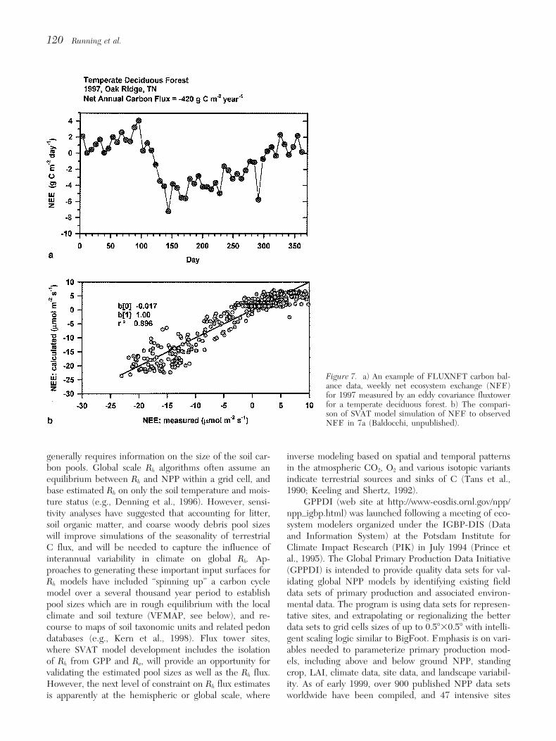
Figure 7. a) An example of FLUXNET carbon bal-ance data, weekly net ecosystem exchange (NEE)for 1997 measured by an eddy covariance fluxtowerfor a temperate deciduous forest. b) The compari-son of SVAT model simulation of NEE to observedNEE in 7a (Baldocchi, unpublished).

generally requires information on the size of the soil car- inverse modeling based on spatial and temporal patternsin the atmospheric CO2, O2 and various isotopic variantsbon pools. Global scale Rh algorithms often assume an

equilibrium between Rh and NPP within a grid cell, and indicate terrestrial sources and sinks of C (Tans et al.,1990; Keeling and Shertz, 1992).base estimated Rh on only the soil temperature and mois-

ture status (e.g., Denning et al., 1996). However, sensi- GPPDI (web site at http://www-eosdis.ornl.gov/npp/npp igbp.html) was launched following a meeting of eco-tivity analyses have suggested that accounting for litter,

soil organic matter, and coarse woody debris pool sizes system modelers organized under the IGBP-DIS (Dataand Information System) at the Potsdam Institute forwill improve simulations of the seasonality of terrestrial

C flux, and will be needed to capture the influence of Climate Impact Research (PIK) in July 1994 (Prince etal., 1995). The Global Primary Production Data Initiativeinterannual variability in climate on global Rh. Ap-

proaches to generating these important input surfaces for (GPPDI) is intended to provide quality data sets for val-idating global NPP models by identifying existing fieldRh models have included “spinning up” a carbon cycle

model over a several thousand year period to establish data sets of primary production and associated environ-mental data. The program is using data sets for represen-pool sizes which are in rough equilibrium with the local

climate and soil texture (VEMAP, see below), and re- tative sites, and extrapolating or regionalizing the betterdata sets to grid cells sizes of up to 0.5830.58 with intelli-course to maps of soil taxonomic units and related pedon

databases (e.g., Kern et al., 1998). Flux tower sites, gent scaling logic similar to BigFoot. Emphasis is on vari-ables needed to parameterize primary production mod-where SVAT model development includes the isolation

of Rh from GPP and Ra, will provide an opportunity for els, including above and below ground NPP, standingcrop, LAI, climate data, site data, and landscape variabil-validating the estimated pool sizes as well as the Rh flux.

However, the next level of constraint on Rh flux estimates ity. As of early 1999, over 900 published NPP data setsworldwide have been compiled, and 47 intensive sitesis apparently at the hemispheric or global scale, where


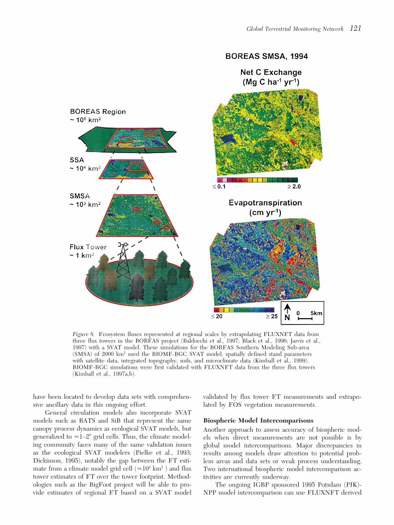
Figure 8. Ecosystem fluxes represented at regional scales by extrapolating FLUXNET data fromthree flux towers in the BOREAS project (Baldocchi et al., 1997; Black et al., 1996; Jarvis et al.,1997) with a SVAT model. These simulations for the BOREAS Southern Modeling Sub-area(SMSA) of 2000 km2 used the BIOME-BGC SVAT model, spatially defined stand parameterswith satellite data, integrated topography, soils, and microclimate data (Kimball et al., 1999).BIOME-BGC simulations were first validated with FLUXNET data from the three flux towers(Kimball et al., 1997a,b).

have been located to develop data sets with comprehen- validated by flux tower ET measurements and extrapo-lated by EOS vegetation measurements.sive ancillary data in this ongoing effort.

General circulation models also incorporate SVATBiospheric Model Intercomparisonsmodels such as BATS and SiB that represent the same

canopy process dynamics as ecological SVAT models, but Another approach to assess accuracy of biospheric mod-generalized to .1–28 grid cells. Thus, the climate model- els when direct measurements are not possible is bying community faces many of the same validation issues global model intercomparisons. Major discrepancies inas the ecological SVAT modelers (Pielke et al., 1993; results among models draw attention to potential prob-Dickinson, 1995), notably the gap between the ET esti- lem areas and data sets or weak process understanding.mate from a climate model grid cell (.104 km2 ) and flux Two international biospheric model intercomparison ac-tower estimates of ET over the tower footprint. Method- tivities are currently underway.ologies such as the BigFoot project will be able to pro- The ongoing IGBP sponsored 1995 Potsdam (PIK)-

NPP model intercomparison can use FLUXNET derivedvide estimates of regional ET based on a SVAT model

122 Running et al.

NPP estimates to test global NPP model estimates at lo- mate (current and projected under doubled CO2), atmo-spheric CO2, and mapped and model-generated vegeta-cations sampled by the network. The website is at http://

gaim.unh.edu/. The 1995 Potsdam NPP model inter- tion distributions. Maps of climate, climate changescenarios, soil properties, and potential natural vegetationcomparison project was an international collaboration that

produced single-year global NPP simulations (Cramer et were prepared as common boundary conditions and driv-ing variables for the models (Kittel et al., 1995). As aal., 1999). There were large discrepancies amongst mod-

els of NPP in northern boreal forests and seasonally dry consequence, differences in model results arose onlyfrom differences among model algorithms and their im-tropics. Over much of the global land surface, waterplementation rather than from differences in inputsavailability most strongly influenced estimates of NPP;(VEMAP, 1995). VEMAP is currently in the second phasehowever, the interaction of water with other multipleof model intercomparison and analysis. The objectives oflimiting resources influenced simulated NPP in a non-Phase 2 are to compare time-dependent ecological re-predictable fashion (Churkina and Running, 1998).sponses of biogeochemical and coupled biogeochemical–VEMAP (http://www.cgd.ucar.edu:80/vemap/) is an on-biogeographical models to historical and projected tran-going multi-institutional, international effort addressingsient forcings across the conterminous United States.the response of terrestrial biogeography and biogeo-Because the VEMAP project has no validation compo-chemistry to environmental variability in climate andnent, interaction with FLUXNET and EOS can provideother drivers in both space and time domains. The ob-direct model validations. (Schimel et al., 1997)jectives of VEMAP are the intercomparison of bio-

geochemistry models and vegetation distribution models(biogeography models) and determination of their sensi- INTERNATIONAL COORDINATIONtivity to changing climate, elevated atmospheric carbon AND IMPLEMENTATIONdioxide concentrations, and other sources of altered forc-ing. The completed Phase 1 of the project was structured Global validation and monitoring cannot be done without

international cooperation that transcends any nationalas a sensitivity analysis, with factorial combinations of cli-

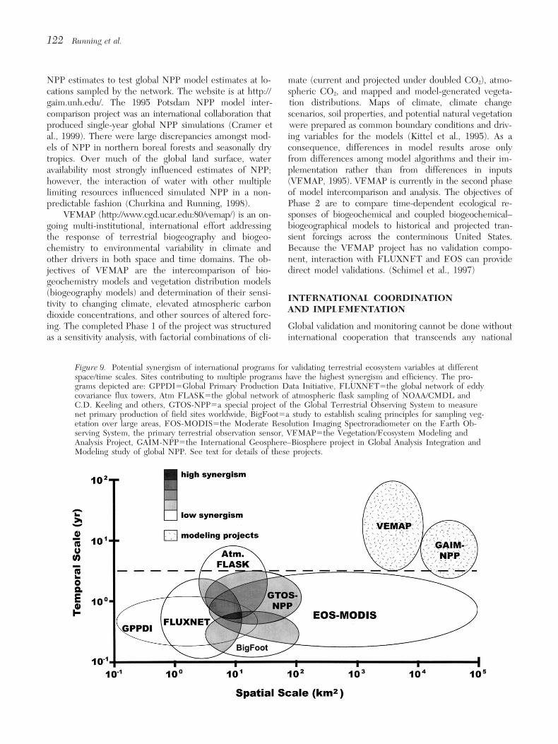
Figure 9. Potential synergism of international programs for validating terrestrial ecosystem variables at differentspace/time scales. Sites contributing to multiple programs have the highest synergism and efficiency. The pro-grams depicted are: GPPDI5Global Primary Production Data Initiative, FLUXNET5the global network of eddycovariance flux towers, Atm FLASK5the global network of atmospheric flask sampling of NOAA/CMDL andC.D. Keeling and others, GTOS-NPP5a special project of the Global Terrestrial Observing System to measurenet primary production of field sites worldwide, BigFoot5a study to establish scaling principles for sampling veg-etation over large areas, EOS-MODIS5the Moderate Resolution Imaging Spectroradiometer on the Earth Ob-serving System, the primary terrestrial observation sensor, VEMAP5the Vegetation/Ecosystem Modeling andAnalysis Project, GAIM-NPP5the International Geosphere–Biosphere project in Global Analysis Integration andModeling study of global NPP. See text for details of these projects.


Table 3. The IGBP Terrestrial Transects Currently Identified

Region Contributing Transects in Initial Set

Humid tropics Tropical forest and its agricultural derivativesAmazon Basin/MexicoCentral Africa/MiomboSoutheast Asia/Thailand

Semiarid tropics Forest–woodland–shrubland (the savannas)Savannas in the long term (West Africa)Kalahari (Southern Africa)Northern Australia Tropical Transect

Midlatitude semiarid Forest–grassland–shrublandGreat Plains (USA)ArgentinaNorth East China Transect

High latitudes Boreal forest–tundraAlaskaBoreal Forest Transect (Canada)ScandinaviaSiberia

agency (Fig. 9). When planning global networks, it is es- four key regions, with three or four existing, planned orproposed transects contributing to the set in each regionsential to recognize that not all facilities have equal levels

of scientific activity; however, all are needed to provide (Table 3).The GTOS-NPP project (website at http://www.fao.adequate global sampling. The Global Terrestrial Ob-

serving System (GTOS) and terrestrial components of org/GTOS/Home.htm) is being coordinated through theinternational U.S. Long Term Ecological Networkthe Global Climate Observing System GCOS have led in

designing consistent international measurements for vali- (LTER) office, http://lternet.edu/ilter/. The goal of theGTOS-NPP project is to distribute the 1km EOS NPPdation and monitoring work (GCOS, 1997). The strategy

for implementing the plan is being developed in con- and LAI products every 8 days to regional networks forevaluation, and after validation, translation of these stan-junction with the World Meteorological Organization

(WMO) and the International GeosphereBiosphere Pro- dard products to regionally specific crop, range, and for-est yield maps for land management applications. Thegramme (IGBP). The plan will provide the necessary

climate requirements for GTOS and the terrestrial re- project will also provide global validation points for landparamatrization in climate and carbon cycle models.quirements for GCOS. See http://www.wmo.ch/web/

gcos/gcoshome.html.Databases and ArchivingTwo core projects of IGBP have been instrumental

in developing coordinated terrestrial systems. BAHC is Establishing data archiving centers is also important forthe original project to suggest FLUXNET, and GCTE international distribution and long-term availability ofhas led in designing the IGBP Terrestrial Transects. data. Several long-term databases are currently beingBoth GAIM and IGAC now are supporting the continu- compiled at the Oak Ridge, Tennessee, USA, DAAC fa-ing development of a global validation and monitoring cility. This data archive facility is home for data fromsystem. Two internationally coordinated activities appear FLUXNET, BigFoot, and GPPDI projects, all that haveready to implement FLUXNET and biospheric monitor- been summarized here (Olson et al., 1999, this issue). Aing activities, the IGBP Transects, and the GTOS-NPP centralized permanently funded data center such as theproject. Oak Ridge DAAC insures continuity, consistency, and

The IGBP Terrestrial Transects, website at: http:// availability of data. However, the proliferation of In-gcte.org/LEMA-IGBP/LEMA-IGBP.html, are a set of in- ternet makes a more distributed array of data archivetegrated global change projects consisting of distributed facilities equally useful if permanent commitments ofobservational studies and manipulative experiments, cou- support are made.pled with modeling and synthesis activities organizedalong existing gradients of underlying global change pa-

CONCLUSIONSrameters, such as temperature, precipitation, and landuse. The IGBP Terrestrial Transects consist of a set of Each of the four monitoring scheme components de-study sites arranged along an underlying climatic gradi- scribed here—flux towers, flask sampling, ecosystement; of order 1000 km in length and wide enough to en- modeling, and EOS satellite data—are a source of con-compass the dimensions of remote sensing images. The sistency checks and validation to the other components.

For example, if [as suggested in Fan et al. (1998)] theinitial set of IGBP Terrestrial Transects are located in

124 Running et al.

Benson, B. J., and MacKenzie, M. D. (1995), Effects of sensorinverse modeling from the flask network suggested a Cspatial resolution on landscape structure parameters. Land-sink on the order of 1–2 Pg C y21 in temperate Northscape Ecol. 10:113–120.America, then results from a sample of flux tower sites

Black, T. A., den Hartog, G., Neumann, H. H., et al. (1996),in that region could confirm that specific sites were largeAnnual cycles of water vapor and carbon dioxide fluxes incarbon sinks, and results from a continental SVAT modeland above a boreal aspen forest. Global Change Biol.initialized and driven by satellite data would support the 2:219–229.

presence of the carbon sink. The achievement of consis- Churkina, G., and Running, S. W. (1998), Contrasting climatetent agreement between the annual global NEE estimate controls on the estimated productivity of global terrestrialfrom the flask network, and from a budget based on a biomes. Ecosystems 1:206–215.spatially distributed SVAT model driven by satellite data, Ciais, P., Tans, P. P., Trolier, M., White, J. W. C., and Francey,

R. J. (1995), A large northern hemisphere terrestrial CO2a spatially distributed model of marine sources and sinkssink indicated by 13C/12C of atmospheric CO2. Science 269:driven by satellite data, and an inventory of anthropo-1098–1102.genic sources, will be an important cross-check.

Cohen, W. B., Fiorella, M., Gray, J., Helmer, E., and Ander-Accurate monitoring of global scale changes in theson, K. (1998), An efficient and accurate method for map-terrestrial biosphere are more critical than ever before.ping forest clearcuts in the Pacific Northwest using LandsatThe Kyoto Protocol signals some of the huge socioeco-imagery. Photogramm. Eng. Remote Sens. 64:293–300.nomic and political decisions that lie ahead, and that will Cohen, W. B., Spies, T. A., and Fiorella, M. (1995), Estimating

rely heavily on quantitatively accurate measures of global the age and structure of forests in a multi-ownership land-biospheric changes. The development of daily satellite scape of western Oregon, U.S.A. Int. J. Remote Sens. 16:earth observations, automated field measurement devices 721–746.such as fluxtowers, powerful ecosystem models summa- Conway, T. J., Tans, P. P., Waterman, L. S., et al. (1994), Evi-

dence for interannual variability of the carbon cycle fromrizing process interactions and high-speed computer net-the National Oceanic and Atmospheric Administration/Cli-working makes a coordinated global biospheric moni-mate Monitoring and Diagnostics Laboratory global air sam-toring program more attainable than ever before. Allpling network. J. Geophys. Res. 99:22,831–22,856.components of the program outlined in this article cur-

Cramer, W., Kicklighter, D. W., Boned, A., et al., and Potsdamrently exist, and primarily need better coordination to95 (1999), Comparing global models of terrestrial net pri-become a global monitoring program. This article is de-mary productivity (NPP): overview and key results. Globalsigned to accelerate that coordination. Change Biol. 5(Suppl. 1):1–15.

Crawford, T. L., Dobosy, R. J., McMillen, R. T., Vogel, C. A.,The primary sponsors of this work have been the U.S. Depart- and Hicks, B. B. (1996), Air–surface exchange measurementment of Energy, National Aeronautics and Space Administra- in heterogeneous regions: extending tower observations withtion Earth Science Enterprise, National Oceanic and Atmo- spatial structure observed from small aircraft. Globalspheric Administration, and the National Science Foundation. Change Biol. 2:275–285.International scientific organizations that have sponsored the Denning, A. S., Fung, I. Y., and Randall, D. (1995), Latitudinalevolution of this program include the International Geosphere–

gradient of atmospheric CO2 due to seasonal exchange withBiosphere Program, and the Global Climate and Terrestrialland biota. Nature 376:240–243.Observing Systems programs of the World Climate Research

Dickinson, R. E. (1995), Land processes in climate models. Re-Program. An early version of this article was presented at themote Sensing Environ. 51:27–38.international FLUXNET meeting in Polson, Montana, USA on

3–5 June 1998. Denning, A. S., Collatz, G. J., Zhang, C., et al. (1996), Simula-tions of terrestrial carbon metabolism and atmospheric CO2

in a general circulation model. Part 1: Surface carbon fluxes.REFERENCES Tellus 48B:521–542.

Fan, S.-M., Goulden, M., Munger, J., et al. (1995), Environ-mental controls on the photosynthesis and respiration of aBakwin, P. S., Tans, P. P., Hurst, D. F., and Zhao, C. (1998),boreal lichen woodland: a growing season of whole-ecosys-Measurements of carbon dioxide on very tall towers: Resultstem exchange measurements by eddy correlation. Oeco-of the NOAA/CMDL program. Tellus 50B:401–415.logia 102:443–452.Baldocchi, D., Hicks, B. B., and Meyers, T. P. (1988), Measur-

Fan, S.-M., Gloor, M., Mahlman, J., et al. (1998), A large ter-ing biosphere–atmosphere exchanges of biologically relatedrestrial carbon sink in North America implied by atmo-gases with micrometeorological methods. Ecology 69:1331–spheric and oceanic CO2 data and models. Science 282:1340.442–446.Baldocchi, D., Valentini, R., Running, S., Oechel, W., and

Farquhar, G. D., Lloyd, J., Taylor, J. A., et al. (1993), Vegeta-Dahlman, R. (1996), Strategies for measuring and modelingtion effects on the isotope composition of oxygen in atmo-carbon dioxide and water vapour fluxes over terrestrial eco-spheric CO2. Nature 363:439–443.systems. Global Change Biol. 2:159–168.

Field, C. B., Behrenfield, M. J., Randerson, J. T., and Falkow-Baldocchi, D. D., Vogel, C. A., and Hall, B. (1997), Seasonalski, P. (1998), Primary production of the biosphere: Inte-variation in carbon dioxide exchange rates above and belowgrating terrestrial and oceanic components. Science 281:a boreal jack pine forest. Agric. Forest Meteorol. 83:147–

170. 237–240.


Field, C. B., Randerson, J. T., and Malmstrom, C. M. (1995), patterns in soil organic carbon pool size in the NorthwesternGlobal net primary production: combining ecology and re- United States. In Soil Processes and the Carbon Cycle (R.mote sensing. Remote Sens. Environ. 51:74–88. Lal, J. M. Kimball, R. Follett, and B. A. Stewart, Eds.),

Foley, J. A., Prentice, C., Namankutty, N., et al. (1996), An CRC Press, Boca Raton, FL, pp 29–43.integrated biosphere model of land surface processes, ter- Kimball, J. S., Thornton, P. E., White, M. A., and Running,restrial carbon balance and vegetation dynamics. Global Bio- S. W. (1997a), Simulating forest productivity and surface–geochem. Cycles 10:603–628. atmosphere carbon exchange in the BOREAS study region.

Frolking, S., Goulden, M. L., Wofsy, S. C., et al. (1996), Mod- Tree Physiol. 17:589–599.eling temporal variability in the carbon balance of a spruce/ Kimball, J. S., White, M. A., and Running, S. W. (1997b),moss boreal forest. Global Change Biol. 2:343–366. BIOME-BGC simulations of stand hydrologic processes for

Global Climate Observing System (GCOS) (1997), GCOS/ BOREAS. J. Geophys. Res. 102(D24):29,043–29,051.GTOS Plan for Terrestrial Climate-Related Observations, Kimball, J. S. Running, S. W., and Saatchi, S. S. (1999), Sensi-Version 2.0 GCOS-32, QMO/TD-No. 796, World Meteoro- tivity of boreal forest regional water flux and net primarylogical Organization, Geneva, Switzerland, 130 pp. production simulations to sub–grid scale landcover complex-

Goulden, M. L., Munger, J. W., Fan, S.-M., Daube, B. C., and ity. J. Geophys. Res., in press.Wofsy, S. C. (1996), Exchange of carbon dioxide by a decid- Kittel, T. G. F, Rosenbloom, N. A., Painter, T. H., Schimel,uous forest: response to interannual climate variability. Sci- D. S., and VEMAP Modeling Participants (1995), Theence 271:1576–1578. VEMAP integrated database for modeling United States

Gower, S. T., Kucharik, C. J., and Norman, J. M. (1999), Di- ecosystem/vegetation sensitivity to climate change. J. Bio-rect and indirect estimation of leaf area index, FAPAR and geogr. 22 (4–5):857–862.net primary production of terrestrial ecosystems. Remote Landsberg, J. J., and Gower, S. T. (1997), Applications of Phys-Sens. Environ. 70:29–51. iological Ecology to Forest Management, Physiological Ecol-

Hollinger, D. Y., Kelliher, F. M., Byers, J. N., Hunt, J. E., ogy Series, Academic, San Diego, CA.McSeveny, T. M., and Weir, P. (1994), Carbon dioxide ex- Lenschow, D. H. (1995), Micrometeorological techniques forchange between an undisturbed old-growth temperate for- measuring biosphere–atmosphere trace gas exchange. Inest and the atmosphere. Ecology 75:134–150. Trace Gases in Ecology (P. Matson and B. Harris, Eds.)

Hunt, E. R., Jr., Piper, S. C., Nemani, R., Keeling, C. D., Otto, Blackwell Science Ltd., Oxford, pp. 126–163.R. D., and Running, S. W. (1996), Global net carbon ex- Melillo, J. M., McGuire, A. D., Kicklighter, A. D., Moore, B.,change and intra-annual atmospheric CO2 concentrations

III, Vorosmarty, C. J., and Schloss, A. L. (1993), Global cli-predicted by an ecosystem process model and three-dimen-mate change and terrestrial net primary production. Na-sional atmospheric transport model. Global Biogeochem.ture 363:234–240.Cycles 10:431–456.

Moncrieff, J. B., Malhi, Y., and Leuning, R. (1996), The propa-IGBP Terrestrial Carbon Working Group (1998), The terres-gation of errors in long-term measurements of land–trial carbon cycle: implications for the Kyoto Protocol. Sci-atmosphere fluxes of carbon and water. Global Changeence 280:1393–1394.Biol. 2:231–240.Jarvis, P. G., Massheder, J. M., Hale, S. E., Moncreif, J. B.,

Moore, C. J. (1986), Frequency response corrections for eddyPayment, R., and Scott, S. L. (1997), Seasonal variation ofcorrelation systems. Boundary Layer Meteorol. 37:17–35.carbon dioxide, water vapor and energy exchanges of a bo-

Myneni, R. B., Keeling, C. D., Tucker, C. J., Asrar, G., andreal black spruce forest. J. Geophys. Res. 102(D24) 28,953–Nemani, R. R. (1997a), Increased plant growth in the north-28,966.ern high latitudes from 1981–1991. Nature 386:698–702.Justice, C. O., Vermote E., Townshend, J. R. G., et al. (1998),

Myneni, R. B., Nemani, R. R., and Running, S. W. (1997b),The Moderate Resolution Imaging Spectroradiometer (MO-Estimation of global leaf area index and absorbed par usingDIS): land remote sensing for global change research. IEEEradiative transfer models. IEEE Trans. Geosci. RemoteTrans. Geosci. Remote Sens. 36:1228–1249.Sens. 35:1380–1393.Keeling, C. D., Bacastow, R. B., Carter, A. F., et al. (1989), A

Oechel, W. C., Vourlitis, G. L., Brooks, S., Crawford, T. L.,three-dimensional model of atmospheric CO2 transportand Dumas, E. (1998), Intercomparison among chamber,based on observed winds, 1. Analysis of observational data.tower, and aircraft net CO2 and energy fluxes measured dur-In Aspects of Climate Variability in the Pacific and theing the Arctic System Science Land–atmosphere–Ice Inter-Western Americas (D. H. Peterson, Ed.), Geophys. Mo-actions (ARCSS-LAII) flux study. J. Geophys. Res. 103nogr., 55, American Geophysical Union, Washington, DC,(D22) 28,993–29,003.363 pp.

Olson, R. J., Biggs, J. M., Porter, J. H., Mah, G. R., andKeeling, C. D., Whorf, T. P., Wahlen, M., and v.d. Plicht, J.Stafford, S. G. (1999), Managing data from multiple disci-(1995), Interannual extremes in the rate of rise of atmo-plines, scales and sites to support synthesis and modeling.spheric carbon dioxide since 1980. Nature 375:666–670.Remote Sens. Environ. 70:99–107.Keeling, R. F., Piper, S. C., and Heimann, M. (1996), Global

Pielke, R. A., Schimel, D. S., Lee, T. J., Kittel, T. G. F., andand hemispheric CO2 sinks deduced from changes in atmo-Zeng, X. (1993), Atmosphere–terrestrial ecosystem interac-spheric O2 concentration. Nature 381:218–221.tions: implications for coupled modeling. Ecol. Model. 67:Keeling, R. F., and Shertz, S. R. (1992), Seasonal and interan-5–18.nual variations in atmospheric oxygen and implications for

Pierce, L. L., and Running, S. W. (1995), The effects of aggre-the global carbon cycle. Nature 358:723–727.Kern, J. S., Turner, D. P. and Dodson, R. F. (1998), Spatial gating sub-grid land surface variation on large-scale esti-

126 Running et al.

mates of net primary production. Landscape Ecol. 10: Tans, P. P., Bakwin, P. S., and Guenther, D. W. (1996), A fea-239–253. sible global carbon cycle observing system: a plan to deci-

Potosnak, M. J., Wofsy, S. C., Denning, A. S., Conway, T. J., pher today’s carbon cycle based on observations. GlobalNovelli, P. C., and Barnes, D. H. (1998), Influence of biotic Change Biol. 2:309–318.exchange and combustion sources on atmospheric CO2 con- Tans, P. P., Fung, I. Y., and Takahashi, T. (1990), Observa-centrations in New England from observations at a forest tional constraints on the global atmospheric CO2 budget.flux tower. J. Geophys. Res., in press. Science 247:1431–1438.

Prince, S. D. and Goward, S. T. (1995), Global primary pro- Thomlinson, J. R., Bolstad, P. V., and Cohen, W. B. (1999),duction: a remote sensing approach. J. Biogeogr. 22: Coordinating methodologies for scaling landcover classifica-815–835. tions from site-specific to global: steps toward validating

Prince, S. D., Olson, R. J., Dedieu, G., Esser, G., and Cramer, global map products. Remote Sens. Environ. 70:16–28.W. (1995), Global Primary Production Data Initiative Proj- Townshend, J. R. C., and Justice, C. O. (1988), Selecting theect description, IGBP-DIS Working Article No. 12, IGBP- spatial resolution of satellite sensors required for globalDIS, Toulouse, France. monitoring of land transformations. Int. J. Remote Sens.

Randerson, J. T., Thompson, M. V., Conway, T. J., Fung, I. Y., 9:187–236.and Field, C. B. (1997), The contribution of terrestrial Turner, D. P., Cohen, W. B., Kennedy, R. E., Fassnacht, K. S.,sources and sinks to trends in the seasonal cycle of atmo- and Briggs, J. M. (1999), Relationships between leaf areaspheric carbon dioxide. Global Biogeochem. Cycles 11: index and Landsat TM spectral vegetation indices across535–560. three temperate zone sites. Remote Sens. Environ. 70:52–68.

Reich, P. B., Turner, D., and Bolstad, P. (1999), An approach Turner, D. P., Dodson, R. D., and Marks, D. (1996), Compari-to spatially-distributed modeling of net primary production

son of alternative spatial resolutions in the application of a(NPP) at the landscape scale and its application in validatingspatially distributed biogeochemical model over complexEOS NPP products. Remote Sens. Environ. 70:69–81.terrain. Ecol. Model. 90:53–67.Ruimy, A., Saugier, B., and Dedieu, G. (1994), Methodology

VEMAP (1995), Vegetation/Ecosystem Modeling and Analysisfor the estimation of terrestrial net primary production fromProject: comparing biogeography and biogeochemistry mod-remotely sensed data. J. Geophys. Res. 99:5263–5283.els in a continental-scale study of terrestrial ecosystem re-Running, S. W. (1998), A blueprint for improved global changesponses to climate change and CO2 doubling. Global Bio-monitoring of the terrestrial biosphere. NASA Earth Obs.geochem. Cycling 9:407–437.10(1):8–11.

Waring, R. H., and Running, S. W. (1998), Forest Ecosystems:Running, S. W., Justice, C. O., Salmonson, V., et al. (1994),Analysis at Multiple Scales, 2nd ed., Academic, San Diego,Terrestrial remote sensing science and algorithms planned370 pp.for EOS/MODIS. Int. J. Remote Sens. 15: 3587–3620.

Waring, R. H., Law, B. E., Goulden, M. L., et al. (1995), Scal-Schimel, D. S. (1998), The carbon equation. Natureing gross ecosystem production at Harvard Forest with re-393:208–209.mote sensing: a comparison of estimates from a constrainedSchimel, D. S., VEMAP Participants, and Braswell, B. H.quantum-use efficiency model and eddy correlation. Plant(1997), Continental scale variability in ecosystem processes:Cell Environ. 18:1201–1213.Models, data, and the role of disturbance. Ecol. Monogr.

White, J. D., Running, S. W., Thornton, P. E., et al. (1998),67:251–271.Assessing simulated ecosystem processes for climate variabil-Tans, P. P. (1998), Oxygen isotopic equilibrium between car-

bon dioxide and water in soils. Tellus 50:163–178. ity at Glacier National Park, USA. Ecol. Appl. 8:805–823.


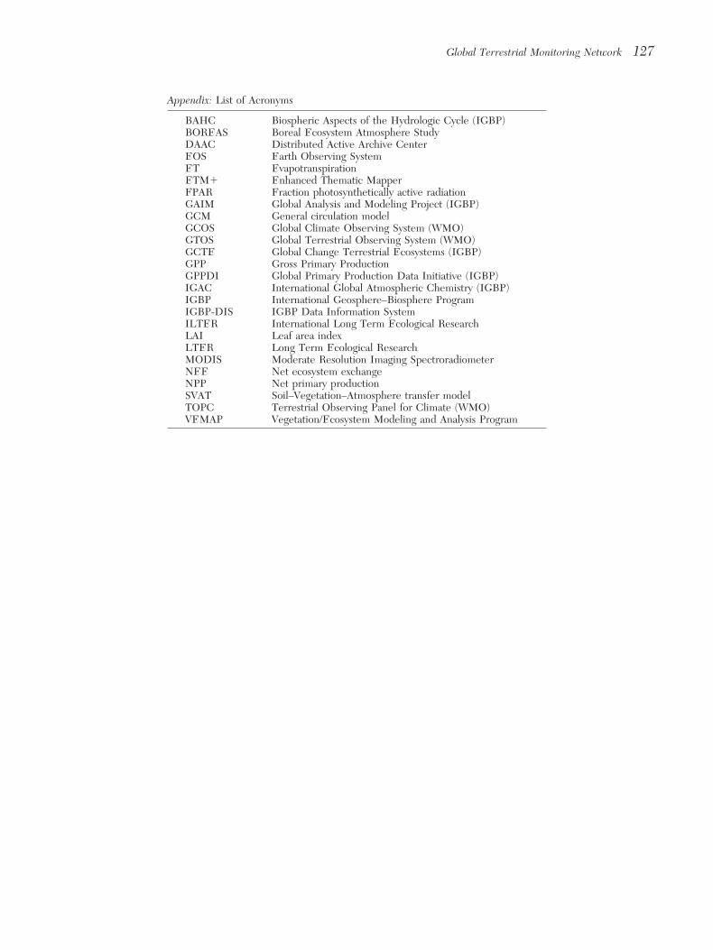
Appendix: List of Acronyms

BAHC Biospheric Aspects of the Hydrologic Cycle (IGBP)BOREAS Boreal Ecosystem Atmosphere StudyDAAC Distributed Active Archive CenterEOS Earth Observing SystemET EvapotranspirationETM1 Enhanced Thematic MapperFPAR Fraction photosynthetically active radiationGAIM Global Analysis and Modeling Project (IGBP)GCM General circulation modelGCOS Global Climate Observing System (WMO)GTOS Global Terrestrial Observing System (WMO)GCTE Global Change Terrestrial Ecosystems (IGBP)GPP Gross Primary ProductionGPPDI Global Primary Production Data Initiative (IGBP)IGAC International Global Atmospheric Chemistry (IGBP)IGBP International Geosphere–Biosphere ProgramIGBP-DIS IGBP Data Information SystemILTER International Long Term Ecological ResearchLAI Leaf area indexLTER Long Term Ecological ResearchMODIS Moderate Resolution Imaging SpectroradiometerNEE Net ecosystem exchangeNPP Net primary productionSVAT Soil–Vegetation–Atmosphere transfer modelTOPC Terrestrial Observing Panel for Climate (WMO)VEMAP Vegetation/Ecosystem Modeling and Analysis Program

a global terrestrial monitoring network integrating tower fluxes

Documents