No. 04‐7 

A General‐Equilibrium Asset‐Pricing Approach to the Measurement of Nominal and Real Bank Output 

J. Christina Wang, Susanto Basu, and John G. Fernald  

Abstract: This paper addresses the proper measurement of financial service output that is not priced explicitly.  It shows how to impute nominal service output from financial intermediaries’ interest income and how to construct price indices for those financial services.  We present an optimizing model with financial intermediaries that provide financial services to resolve asymmetric information between borrowers and lenders.  We embed these intermediaries in a dynamic, stochastic, general‐equilibrium model where assets are priced competitively according to their systematic risk, as in the standard consumption capital‐asset‐pricing model.  In this environment, we show that it is critical to take risk into account in order to measure financial output accurately.  We also show that even using a risk‐adjusted reference rate does not solve all the problems associated with measuring nominal financial service output.  Our model allows us to address important outstanding questions in output and productivity measurement for financial firms, such as: (1) What are the correct “reference rates” to use in calculating bank output?  In particular, should they take account of risk? (2) If reference rates need to be risk‐adjusted, does it mean that they must be ex ante rates of return?  (3) What is the right price deflator for the output of financial firms?  Is it just the general price index?  (4) When—if ever—should we count capital gains of financial firms as part of financial service output? 

JEL Codes: G2, G21, E01, E44  

J. Christina Wang is an Economist at the Federal Reserve Bank of Boston, Susanto Basu is Professor of Economics at the University of Michigan and Research Associate at the NBER, and John G. Fernald is Senior Economist and Economic Advisor at the Federal Reserve Bank of Chicago .  Their email addresses are christina.wang@bos.frb.org, sbasu@umich.edu, and jfernald@frbchi.org, respectively.  This paper, which may be revised, is available on the web site of the Federal Reserve Bank of Boston at http://www.bos.frb.org/economic/wp/index.htm.  The views expressed in this paper are solely those of the authors and do not reflect official positions of the Federal Reserve Bank of Boston or the Federal Reserve System.  This paper was prepared for the CRIW conference on Price Index Concepts & Measurement, Vancouver, June 28‐29, 2004.  We thank Erwin Diewert, Dennis Fixler, Charles Hulten, Alice Nakamura, Emi Nakamura, Marshall Reinsdorf, Paul Schreyer, Jack Triplett, and Kim Zieschang for helpful discussions and Felix Momsen for data.  This version: October 15, 2004         

2

In many service industries, measuring real output is a challenge because it is difficult to

measure quality-adjusted prices. Financial services, however, lack even an agreed-upon

conceptual basis for measuring nominal let alone real output. In this paper, we address this

problem and propose a resolution of some major long-standing debates on how to measure bank

output.1 We present a dynamic, stochastic, general equilibrium (DSGE) model in which nominal

and real values of bank output—and, hence, the price deflator—are clearly defined. We then

assess the adequacy of existing national accounting measures in a fully-specified DSGE setting.

Our model is a general-equilibrium extension of Wang’s (2003a) partial-equilibrium framework,

and it validates Wang’s proposed measure of real bank service flows.

Conceptually, the most vexing measurement issue arises because banks and other financial

service providers often do not charge explicit fees for services, but rather incorporate the charges

into an interest rate margin––the spread between the interest rates they charge and pay. The

System of National Accounts 1993 (SNA93) thus recommends measuring these “financial

intermediation services indirectly measured” (FISIM) using net interest: “the total property income

receivable by financial intermediaries minus their total interest payable, excluding the value of any

property income receivable from the investment of their own funds.”2 Theoretical basis for using

net interest is found in the so-called user-cost approach to banking, which interprets the interest

rate spread as banks’ unit income net of the “user cost” of money.3 As a practical matter, the SNA

approach thus more or less equates nominal output from FISIM with the net interest income that

flows through banks.

Wang (2003a), however, shows that the net interest contains not only the nominal

compensation for bank services but also the return to the systematic risk in bank loans. Wang

(2003a) then argues forcefully that the risk-related return should be excluded from bank output. In

particular, if one aims to account consistently for both banks’ real service flows and the output of

firms that borrow from banks or bond markets, then one should not count the risk premium as

1 For a recent sample, see chapter 7 in Triplett and Bosworth (forthcoming), the comment on that chapter by Fixler (2003), and the authors’ rejoinder. 2 SNA 1993, paragraph 6.125. 3 See, for example, Fixler and Zeischang (1992). Important contributors to the user-cost approach also include Diewert (1974, 2001), Barnett (1978), and Hancock (1985).

3

part of bank output. In essence, the user cost of money should be adjusted for risk, since modern

finance theories of asset pricing demonstrate that the required rate of return depends on risk. The

general-equilibrium model here verifies the partial-equilibrium conclusion reached by Wang

(2003a), as we show below.

The conclusion that one should not include the risk premium in bank output is fully

consistent with the user-cost approach. Both our model and Wang (2003a) work within the user-

cost framework, as both recognize that banks’ optimal choice of interest rates must cover the

opportunity cost of funds as well as the cost of the implicit services provided. The Wang “service

flow” measure of nominal bank output thus also reflects total income net of the opportunity cost of

funds—but it shows that the cost of funds must be adjusted for risk. Wang (2003a) pins down the

cost of funds by applying standard finance theories of asset pricing; the version of the user-cost

approach used in the banking literature by itself provides no theoretical guidance for determining

the opportunity cost of funds. Our general-equilibrium model further endogenizes the cost of

funds, which Wang (2003a) takes as exogenously given by financial markets. As such, both our

model and Wang’s (2003a) approach complement and extend the user-cost approach.

In implementation, SNA93 does not allocate the FISIM to specific sectors and thus does not

distinguish services to borrowers from services to depositors. As a refinement, the 2003 U.S.

National Income and Product Accounts (NIPA) benchmark revision divides banks’ overall

implicitly priced services between borrowers and depositors. The revised measure imputes the

nominal value of services to borrowers as the volume of interest -earning assets times the difference

between the (average) lending rate and a reference rate—the user cost of funds. Likewise, it

imputes nominal output of services to depositors as the volume of deposits times the difference

between a reference rate and the (average) deposit rate, that is, depositors’ foregone interest (Fixler

et al. 2003).

Clearly, the challenge concerning nominal output is to decide on the reference rates. NIPA

uses a risk-free rate for both borrower and depositor services. But our model shows that the

appropriate reference rate for borrowers is not a risk-free rate. Instead, as Wang (2003a) argues, it

is a rate that incorporates the systematic risk of a bank’s loan portfolio, since the cost of funds is

risk-dependent. The obverse is that the imputed value of banks’ implicit borrower services

4

excludes the risk premium. The premium represents compensation for bearing systematic risk,

and thus is part of the property income that flows through the bank to the bank’s shareholders and

certain debt-holders (for example, bondholders and, in countries without deposit insurance,

depositors).

It is intuitive that this risk-based income flow does not, conceptually, represent bank

output. Consider the issue from the point of view of borrowers. Suppose two firms seek to obtain

additional financing. They are identical except that, at the margin, one chooses to borrow in the

bond market whereas the other chooses to borrow from a bank. The bond-financed firm offers an

expected return equal to the risk-free rate plus a risk premium; if investors were risk-neutral or the

firm’s risk were entirely idiosyncratic, the risk premium would be zero and the bond would offer

just the risk-free rate. If there are no transactions costs, it is clear that this entire return represents

the value added of the borrower, not the value added of the financial sector.

Now consider the bank-financed firm. To keep things extremely simple, suppose that

banks hire no labor or capital to produce any services whatsoever. They are merely an accounting

device that records loans (perhaps funded by bank shareholder equity) to borrowers. Since they

provide no screening, monitoring, or other services, they charge the risk -free interest rate plus a

risk premium. Indeed, one would expect it to be the same risk premium as the bond-financed

firm, since the risk is the same and there is no arbitrage in equilibrium. (Note that in equilibrium,

bank shareholders are indifferent between holding shares in the bank or buying the bonds issued

by the bond-financed firm). But NIPA would attribute positive value added to a “bank” equal to

the risk premium times the face value of the loan, even though, by assumption, the bank does

nothing! (Indeed, the bank produces this “output” with no capital or labor input, so it appears

infinitely productive.)

Conceptually, one would want to treat these two firms symmetrically, since they are

identical apart from an arbitrary and (to the firm) irrelevant choice about the source of financing.

But under current accounting conventions, they appear to have different value added, inputs of

financial services, and productivities. In contrast, the approach we recommend would treat the

two firms symmetrically by excluding the risk premium from the bank’s nominal financial

5

output—a premium the borrowing firm must pay whether it is financed by a bank or through

bonds.

Thus, the national accounting measure generates inconsistent results even in the very

simplest of possible models, where banks produce no services that use labor and capital. Our

model, like Wang’s (2003a), shows that the conceptual inconsistency extends to a more realistic

case where banks provide actual services. Hence, our model provides a detailed counter-example

to the use of the entire interest margin as a general measure of bank output. As a special case, the

NIPA measure can arise in our model, but only when bank loans have no systematic risk.

Unfortunately, the special case seems unlikely to be empirically relevant.

The model also provides potential insight into measuring real output and, hence, the

banking price deflator. The U.S. accounts measure real bank output using indices of bank

activities as measured by the Bureau of Labor Statistics (Technical Note, 1998). Given data

limitations, these measures are, however, occasionally crude along some dimensions, for example,

number of loans and number of checks written. Again, given data limitations, these imperfect

measures are then weighted in a relatively ad hoc manner. The practical limitations include the

lack of data as well as the lack of clear conceptual guidance on how to weight different activities in

the absence of clearly attributable nominal shares in cost or revenue.

Quantitatively, the potential mismeasurement under the current system is large. In 2001,

commercial banks in the United States had nominal output of $187 billion.4 Of this total, about half

is final consumption; the other half is intermediate services provided to businesses. The results of

this paper imply that the measured figures overstate true output. Our paper is theoretical and can

only sign the bias, but the empirical implementation of similar concepts by Wang (2003b) suggests

that NIPA output measures for the banking industry may be about 20 percent too high. This

reflects both an overestimate of lending services provided to consumers (hence, an overstatement

of GDP) and an overestimate of intermediate services provided to firms (which does not overstate

GDP, but distorts measures of industry output and productivity).

These biases, while large in dollar terms, are obviously small relative to U.S. GDP or to the

4 Figures are from Fixler, Reinsdorf, and Smith (2003) and reflect the December 2003 comprehensive revisions.

6

total output of the industries that purchase banking services. However, similar considerations

apply to measuring the output of financial services more generally, so the full set of NIPA

corrections suggested by our paper is substantial. Furthermore, banking contributes a larger share

to GDP in some other countries. For example, banking services account for 37 percent of

Luxemburg’s exports, which in turn are 150 percent of GDP. Thus, our work suggests that

Luxemburg’s GDP could be overstated by about 11 percent—surely substantial by any measure.

In addition, growth rates are also biased by the likely time-varying nature of risk premia.

(See Wang, 2003b.) The growth-rate bias is exacerbated during transitions such as those taking

place now, when banks are securitizing an ever-larger fraction of their loans. For example, as

banks securitize more loans, they move the “risk premium” off their books, even if they continue

to provide substantially the same real services, for example, screening and monitoring loans.

Several studies find that financial services contributed importantly to the post-1995 U.S.

productivity growth revival, 5 so it is important to measure the growth as well as the level of these

sectors’ outputs correctly.

Our explicit DSGE model with an active banking sector also enables us to realize insights

that would be difficult to obtain in a less-completely-specified setting. In particular, our model

elucidates two other problems with using net interest income to measure nominal service flows,

which may further bias the national accounting measure of bank output. Being dynamic, our

model highlights the potential timing mismatch between when a service is performed (for

example, screening when a loan is originated) and when that service is compensated (with higher

interest payments over the lifetime of the loan). Being stochastic, the model points out that the

expected nominal output of monitoring services (services that are performed during the lifetime of a

loan, after it is originated) can be measured from ex ante interest rate spreads, but the actual

monitoring services produced are difficult to measure from ex post revenue flows.

In general, our use of a dynamic general equilibrium model, although relatively rare in the

measurement literature, offers several advantages for studying measurement issues. First, and

most generally, national income accounting is inherently an economy-wide activity, imposing a set

of adding-up constraints that must hold in the aggregate. General-equilibrium models impose the

5 Basu et al. (2003), among many others, come to this conclusion.

7

same restrictions, but also incorporate economic behavior that is optimized under these and other

constraints. By applying actual national income accounting procedures to the variables generated

by the model, we can ask whether and under what conditions the objects measured in the national

accounts correspond to the economic concepts we want to measure.

Second, and more specific to our current project, the study of banking intrinsically concerns

both goods- and asset-market interactions among different agents and thus inherently draws on

diverse economic concepts. Those interactions endogenously determine goods prices, quantities,

and interest rates. (See Kwark, 2002, for a similar model.) This nexus of economic connections is

best studied in a general-equilibrium setting, since it ensures the comprehensive consideration of

all the key elements of an economy. For example, one needs to specify an environment in which

intermediation is necessary: In the model, households cannot or will not lend directly to firms for

well-specified informational problems. We also need to specify how banks then produce real

intermediation services and what determines required rates of return on bank assets.

A major contribution of the DSGE model is to endogenize the risk premium of loans that

fund corporations’ capital, as well as the required rate of return on banks’ equity. Our model is

basically a real business-cycle model, augmented to take account of the information asymmetry

between the users and the suppliers of funds. It is thus along the line of models in Bernanke and

Gertler (1989) and Bernanke, Gertler, and Gilchrist (1999), among others. The special feature of our

setup is that we explicitly model both screening and monitoring activities by financial

intermediaries, both of which are needed to resolve the asymmetric information prob lem in the

investment process. The purpose is to highlight the proper measurement of bank service output in

both nominal and real terms. Hence, the model also provides a framework with which to think

about constructing price indices for banking services.

Furthermore, our service-flow perspective yields insights into the empirical microeconomic

literature on banking. That literature often takes as bank output the dollar value of interest-

bearing assets (loans plus market securities) on bank balance sheets deflated by some general price

index. The service-flow perspective takes bank output as the production of financial services, an

act that consumes real inputs of capital and labor. In our model, there is no definitive link between

bank services and the dollar value of interest -bearing assets. Thus, the model suggests that there is

8

no general theoretical foundation for using the book value of interest-bearing assets as a measure

of output. Think again of the bank that does nothing. By construction, this bank produces no

output; but since it holds loans, the micro approach would credit it with producing real output.

(Again, the bank will appear infinitely productive.)

To avoid unnecessary complexity, we abstract from various activities banks undertake

(mainly transactions services to depositors) as well as from realistic complications (for example,

deposit insurance and taxes). Many of these abstractions could be incorporated, and it seems

likely that most will not interact in important ways with the issues we address here.

For example, our approach extends naturally to valuing activities by banks other than

making loans and taking deposits, such as underwriting derivatives contracts and other exotic

financial instruments. We present one such example in the paper. Thus, our paper begins the

process of bringing measurement into line with the new roles that banks play in modern

economies, as discussed by Allen and Santomero (1998, 1999).

Nevertheless, the reader might be tempted to ask whether conclusions drawn from our

bare-bones model apply to the far more complex real world. But the real question is the opposite.

Our model provides a controlled setting where we know exactly what interactions take place and

what outcomes result. Even in this relative simple setting, current methods of measuring nominal

and real bank output generate inconsistent results that can be economically substantial. Then,

what chance is there that these methods will magically succeed in the far more complex world?

The paper is organized in four main sections. Sections I and II present the basic setup of

the model with minimal technicality, to build intuition for the economic reasoning behind our

conclusions. (We put the rigorous solution of the model in Appendix 1.) Section I solves the

model with symmetric information between borrowers and lenders and uses this simple setup to

show by example that existing proposals for measuring bank output are flawed. Section II

introduces asymmetric information, and assumes that banks and rating agencies have a

technological advantage in resolving such asymmetries. In this setting financial institutions

actually provide real services, and this section derives the correct, model-based measure of bank

output. Section III discusses implications of the model for the measurement of nominal and real

9

output of the financial sector. Section IV discusses several important extensions of the model.

Section V concludes, and suggests priorities for future research and data collection.

I. The Model with Symmetric Information

A. Overview

Our model has three central groups of agents: households, who supply labor and who

ultimately own the economy’s capital; entrepreneurs, who hire workers and buy capital to operate

projects; and competitive financial institutions (banks and rating agencies) that resolve information

problems between the owners and the final users of capital. It also has a bond market, in which

entrepreneurs can issue corporate debt.

Households are the only savers in this economy and thus the ultimate owners of all capital.

Their preferences determine the risk premium on all financial assets in the economy, and their

accumulated saving determines the amount of capital available for entrepreneurs to rent in a given

period.

Entrepreneurs operate projects that produce the economy’s final output. There is only one

homogeneous final good, sold in a competitive market, which can be consumed or invested.

Entrepreneurs’ projects differ from one another since the entrepreneurs differ in their ability levels

(or, equivalently, in the intrinsic productivity of their projects). The technology for producing final

goods in any project has constant returns to scale. Thus, without asymmetric information, the

social optimum would be to give all the capital to the most efficient project. But we assume that

entrepreneurs face a supply curve for funds that is convex in the amount borrowed. 6 As we

discuss below, we assume that entrepreneurs are born without wealth—they are the proverbial

impoverished geniuses, whose heads are full of ideas but whose purses hold only air—so that, one

way or another, they will need to obtain funds from households.

6 Given that all entrepreneurs are borrowing without collateral, this seems quite realistic. Our specific modeling assumption is that the cost of screening is convex in the size of the project, but other assumptions—such as leveraging each entrepreneur’s net worth with debt—would also lead to this result. See Bernanke, Gertler, and Gilchrist (1999).

10

The focus of this paper is on how the entrepreneurs obtain the funds for investment from

households, and the role of financial intermediaries in the process. A large literature on financial

intermediation explains (in partial equilibrium) financial institutions’ role as being to resolve

informational asymmetries between the ultimate suppliers of funds (that is, the households in our

model) and the users of funds (that is, the entrepreneurs who borrow to buy capital and produce).

We incorporate this result into our general-equilibrium model.7

In this paper, we consider both types of information asymmetry—hidden information and

hidden actions. Households face adverse selection ex ante as they try to select projects to finance:

They know less about the projects (for example, default probabilities under various economic

conditions) than entrepreneurs, who have an incentive to understate the risk of their projects.

Moral hazard arises ex post as savers cannot perfectly observe borrowers’ actions, which are often

detrimental to savers given the typical conflict between principals and agents. For instance, an

entrepreneur might appropriate project payoff for personal gains, or substitute a more risky project

that heightens the default probability while enhancing his expected residual payoff. Such

information asymmetries distort capital markets and result in deadweight loss, as in this model.

Thus, the third group of actors in our model are banks and bank-like institutions which

exist (in the model and, largely, in practice) in order to mitigate these information problems. 8 We

focus on two specific services provided by banks: They screen entrepreneurs to lessen (in our

model, to eliminate) entrepreneurs’ private information about the viability of their projects, and

they monitor outcomes to discover and curb entrepreneurs’ hidden actions. 9 To conduct screening

and monitoring, intermediaries engage in a production process that uses real resources of labor,

capital, and an underlying technology. The production process is qualitatively similar to

7 Most other general-equilibrium models (all on growth or business cycles) abstract from this issue: Implicitly, households own and operate the firms directly so that there are no principal-agent problems. 8 Financial institutions prevents market breakdown (such as in Akerlof, 1970), but cannot eliminate deadweight loss. Another major function of banks is to provide services to depositors, as discussed in the introduction. But we omit them from the formal model, since their measurement is less controversial and has no bearing on our conclusion about how to treat risk in measuring lending services. Yet, we note practical measurement issues about them in Section III. 9 Many studies, all partial-equilibrium analyses, analyze the nature and operation of such financial intermediaries. For example, Leland and Pyle (1977) model banks’ role as resolving ex ante adverse selection in lending; Diamond (1984) studies delegated monitoring through banks; Ramakrishnan and Thakor (1984) look at non-depository institutions.

11

producing other information services such as consulting and data processing.10

We would note that we call the financial intermediaries “banks” mainly for convenience,

even though the functions they perform have traditionally been central to the activities of

commercial banks. But the analysis is general, as we will show that loans subject to default are

equivalent to a risk-free bond plus a put option. So our analysis also applies to implicit bank

services associated with other financial instruments, as well as to other types of intermediaries,

such as rating agencies and finance companies.

We assume that banks and other financial-service providers are owned by households and

are not subject to informational asymmetries with respect to households. 11 Banks act as a

“conduit,” albeit an active one, channeling funds from households to entrepreneurs and the

returns back to households.

As suppliers of funds, households demand an expected rate of return commensurate with

the systematic risk of their assets. This is, of course, true in any reasonable model with investor

risk aversion, regardless of whether there are informational asymmetries. Banks thus must ensure

that the interest rate charged compensates their owners, the households, with the risk-adjusted

return in expectation. Banks must also ensure that they charge explicit or implicit fees to cover the

costs incurred by screening and monitoring.

The primary focus of this paper is to determine how to measure correctly the nominal and

real service output provided by these banks when the services are not charged for explicitly but

implicitly in the form of higher interest rates. Hence, we need to detail the nature of the contract

between entrepreneurs and banks, since that determines the interest rates banks charge. Indeed,

most of the complexity in the formal model in Appendix 1 comes from the complexity of

specifying the interest rate charged under the optimal debt contract and from decomposing total

interest income into compensation for bank services—screening and monitoring—and a risk-

10 Only a handful of studies analyze the effects of financial intermediaries on real activities in a general equilibrium framework. None of them, however, considers explicitly the issue of financial intermediaries’ output associated with the process of screening and monitoring, nor the properties of the screening and monitoring technology. 11 We could extend our model to allow for this two-tier information asymmetry, at the cost of considerable added complexity. We conjecture, however, that our qualitative results would be unaffected by this change.

12

adjusted return for the capital that households channel to firms through the bank. The payoff from

this complexity is that the model provides definite insights on key measurement issues.

For the most part, we try to specify the incentives and preferences of the three groups of

agents in a simple way, in order to focus on the complex interactions among the agents. We now

summarize the key elements of the incentives and preferences of each agent to give the reader a

working knowledge of the economic environment. We then derive the key first -order conditions

for the optimal pricing of risky assets, which must hold in any equilibrium, to draw implications

from the model that are crucial for measurement purposes. At the end of this section, the reader

may proceed to the detailed discussion of the model that follows in Appendix 1, or proceed to

Section III to study the implications for measurement.

B. Households

We assume households are infinitely lived and risk averse. For most of the paper, we

assume that households can invest their wealth only through a financial intermediary, because

they lack the ability to resolve information asymmetries with entrepreneurs directly. In contrast,

households own and have no informational problems with respect to the intermediaries. All

households are identical, and they maximize the expected present value of life-time utility—here

expressed in terms of a representative household:

( )0,1s H

t t s t ssE V C Nρ

∞+ +=

− ∑ (1)

subject to the budget constraint: HtC = WtNt + Πt + 1

HtR +

% Xt – Xt+1. (2)

HtC is the household’s consumption, Nt is its labor supply, and ρ is the discount factor. Et(.) is the

expectation given the information set at time t. We assume that the utility function V(.) is concave

and that (0)V ′ = ∞ . Wt is the wage rate, Xt represents the household’s total assets (equal to the

capital stock in equilibrium), and Πt is pure economic profit received from ownership of financial

intermediaries (equal to zero in equilibrium, since we assume that this sector is competitive). 1HtR +

%

is the ex post gross return on the household’s asset portfolio (real capital, lent to various agents to

enable production in the economy). Corresponding to the ex post return is an expected return—the

13

required rate of return on risky assets, which we denote 1HtR + . This is a key interest rate in the

following sections, so we discuss it further.

The consumer’s intertemporal first-order condition for consumption (the Euler equation) is:

( ) ( )1 1 1,1 E ,1H H HC t t t C t t tV C N V C N Rρ + + + − = −

% , (3)

where VC is the partial derivative of utility with respect to consumption. The economic meaning is

that the loss in utility from reducing consumption at time t must equal the gain from investing that

saving in the asset and enjoying the payoff at time t+1. Since future returns and consumption are

unknown, the gain is expected.

Define the intertemporal pricing kernel (also called the stochastic discount factor), mt+1, as

( )( )

1 11

,1

,1

HC t t

t HC t t

V C Nm

V C N

ρ + ++

−≡

−. In this notation, equation (3) implies the basic asset-pricing equation of

the Consumption-based Capital Asset Pricing Model (CCAPM):

( )1 1 1Ht t tE m R+ + =% . (4)

Now suppose a one-period asset whose return is risk-free because it is known in advance.

Clearly, for this asset, the rate of return 1f

tR + satisfies ( ) ( )1 1 1 1 1f ft t t t t tE m R R E m+ + + += = . So,

( )11

1.f

tt t

RE m+

+

= (5)

As is standard in a CCAPM model, the Euler equation (3) allows us to derive the risk-free rate even

if no such asset exists—which is the case in our economy, where the only asset is risky capital. 12

From (4) and (5), the gross required (expected) rate of return on the risky asset, 1HtR + , is:

( ) ( )1 1 1 1 11 cov ,H H f Ht t t t t t tR E R R m R+ + + + + ≡ = −

% % , (6)

12 Any asset-pricing model derives the price of an asset, and thus its implied rate of return, from the equilibrium condition that the net demand for an asset—the amount of the asset demanded minus the amount issued by economic agents—must equal the existing supply. In the case of an asset that does not exist, the supply is zero—which implies that the price must be precisely chosen so that the net demand is also zero. This proposition is easily proved by contradiction. If the risk-free return were higher than this implied rate, every consumer would want to buy such an asset, and if it were lower, every consumer would issue it, and neither situation can be an equilibrium. Assets are qualitatively different from other goods in that economic agents can create them costlessly at will, so the fact that the initial supply is zero does not lead to any pathology. For more discussion, see Cochrane (2001, ch. 2).

14

where covt is the covariance conditional on the information set at time t. The risk premium then

equals

( )1 1 1 1 1cov ,H f f Ht t t t t tR R R m R+ + + + +− = − % .

Thus, given an expected time path for consumption, equation (6) defines the required

return for the portfolio of risky assets that households own. As in the standard CAPM, what

matters is the covariance of the asset return with an aggregate or systematic factor.13 In general,

equation (6) says that assets whose returns covary positively with consumption should have

higher average (required) returns (since they will covary negatively with the marginal utility of

consumption). To provide a concrete example, suppose ( ) ( ) ( ),1 ln ln 1H Ht t t tV C N C Nζ− = + − . In

this log utility case, 11

EHt

t t Ht

Cm

Cρ

++

≡

. It is easy to verify that an asset whose return covaries

positively with consumption has a negative covariance with m, and thus by equation (6) must offer

a rate of return exceeding the risk-free rate. 14

Note that when 1HtR + is the required rate of return on risky debt (for example, loans), that is,

subject to a probability that borrowers will default, there is a subtle but important conceptual

difference between 1HtR + and the interest rate that is charged on loans—the rate that a borrower must

pay if he is not in default. To illustrate in a simple example, suppose there is probability p that a

borrower will pay the interest rate charged (call it 1tR + ), and probability (1 – p) otherwise, in which

case lenders get nothing. Then 1tR + must satisfy

( )1 1 1 11 0 / .H Ht t t tp R p R R R p+ + + ++ − = ⇒ =i i

So 1tR + exceeds the required return 1HtR + ; the margin 1 1

Ht tR R+ +− is the so-called default premium.

Thus, 1tR + differs from the risk -free rate for two reasons. First, there is the default premium. The

13 However, the standard CAPM simply assumes that the relevant factor is the return on the market portfolio. But deriving the relationship from first principles shows that what should matter is the covariance of the return with the marginal utility of consumption, since people ultimately care about welfare, not wealth. (Note that the risk “premium” can in fact be negative in the case of a “negative-beta” asset.) 14 An interesting implication of (6) is that an asset whose return is volatile but uncorrelated with consumption should yield just the risk-free rate! The reason is that the volatility does not represent systematic risk—the risk in holding that asset can be diversified away—and thus it is not risky in the sense of being correlated with marginal utility.

15

borrower repays nothing in bad states of the world, so he must pay more in good states to ensure

an adequate average return. Second, there is a risk premium, as above. The risk premium exists if

the probability of default is correlated with consumption (or more precisely, with the marginal

utility of consumption). If defaults occur when consumption is already low, then they are

particularly costly in utility terms. Thus, the consumer requires an extra return, on average, to

compensate for bearing this systematic, non-diversifiable risk.

In addition to the intertemporal Euler equation, consumer optimization requires a static

tradeoff between consumption and leisure within a period:

( ) ( ),1 ,1H Ht C t t N t tW V C N V C N− = − − . (7)

In equilibrium, households’ assets equal the total capital stock of the economy: Xt = Kt.

The capital stock evolves in the usual way:

( )1 1t t tK K Iδ+ = − + .

Capital is used by intermediaries to produce real financial services, or is bought by firms for

production.15

C. Entrepreneurs

Each entrepreneur owns and manages a non-financial firm that invests in one project,

producing the single homogeneous final good and selling it in a perfectly competitive market. So

entrepreneur, firm, and project are all equivalent and interchangeable in this model.

Entrepreneurs are a set of agents distinct from households in that each has a lifespan of only two

periods, coinciding with the duration of a project. Thus, there are two overlapping generations of

entrepreneurs in each period. The same number of entrepreneurs are born and die each period, so

the fraction of entrepreneurs is constant in the total population of agents.

The reason for having short-lived entrepreneurs in the economy is to create a need for

external financing and thus for screening and monitoring by financial intermediaries. Long-lived

entrepreneurs could accumulate enough assets to self-finance all investment, without borrowing

15 Since we have assumed identical households, we abstract from lending among households (for example, home mortgages).

16

from households. In addition, by having each borrower interact with lenders only once, we avoid

complex supergame Nash equilibria where entrepreneurs try to develop a reputation for being

“good risks” in order to obtain better terms from lenders.

We assume that entrepreneurs, like households, are risk averse. 16 But we abstract from the

issue of risk sharing and assume that the sole income an entrepreneur receives is the residual

project return, if any, net of debt repayment.17 That also means entrepreneurs have no initial

endowment.18 In choosing project size in the first period, entrepreneurs seek to maximize their

expected utility from consumption in the second period, which is the only period when they

consume. Thus, the utility of entrepreneur i born at time t is

( ) ( ),1 , where 0, 0, and 0 0.E i

tU C U U U+ ′ ′′> < = (8)

We denote entrepreneurs’ aggregate consumption by EtC , which is the sum over i of ,E i

tC .

Firms differ only in their exogenous technology parameters. Denote the parameter 1itA + , for

a firm i created in period t, since the owner produces in the second period—t+1. We assume that

1itA + = 1

i itz A + , where At+1 is the stochastic aggregate technology level in period t+1, and zi is i’s

idiosyncratic productivity level, drawn at time t when the owner is born. zi is assumed to be i.i.d.

across firms and time, with bounded support, and independent of At+1, with E(zi) = 1. Conditional

on zi, the firm borrows to buy capital from the households at the end of period t. In keeping with

our desire to study banking operation in detail, we assume that lenders offer borrowers a standard

debt contract. (We discuss the borrowing process, first under symmetric information and then

under asymmetric information, in the next several sub-sections.)

16 If entrepreneurs were risk-neutral, they would insure the households against all aggregate shocks, leading to a degenerate—and counterfactual—outcome where lenders of funds would face no aggregate risk. 17 In fact, this model implicitly allows for the sharing of project-specific risk (that is, zi below) across entrepreneurs (for example, through a mutual insurance contract covering all entrepreneurs), as all the results would remain qualitatively the same. The model assumes that there is no risk sharing between entrepreneurs and households, because the only contract that lenders offer borrowers is a standard debt contract. Given our desire to study banks, this assumption is realistic. 18 The assumption of zero endowment is mainly to simplify the analysis. Introducing partial internal funds, for example, with entrepreneurs’ own labor income, affects none of the model’s conclusions. One potential problem with zero internal funds is that it gives entrepreneurs incentive to take excessive risk (that is, adopting projects with a high payoff when successful but possibly a negative net present value), but we rule out such cases by assumption. The usual principal-agent problem between shareholders and managers does not arise here because entrepreneurs are the owners-operators.

17

The aggregate technology level ( 1tA + ) is revealed at the start of period t+1, and it determines

1itA + (= 1

itz A + ). But since 1tA + is unknown when the capital purchase decision is made, there is a risk

involved for both the borrower and the lender. Conditional on 1itA + and the precommitted level of

capital input, the firm hires the optimal amount of labor at time (t+1)’s going wage, and production

takes place. Entrepreneurs then pay their workers, sell their capital back to households, pay the

agreed-upon interest, and consume all the output left over. See Figure 1 for a time line laying out

the sequence of events across two periods.

If a bad realization of 1tA + leaves an entrepreneur unable to cover the gross interest on his

borrowed funds, he declares bankruptcy. The lenders (households) seize all of the assets and

output of the firm left over after paying the workers, which will be shown to be less than what the

lenders are owed and expect to consume. Entrepreneurs are left with zero consumption, less than

what they expected, as well. The risk to both borrowers and lenders is driven by the aggregate

uncertainty of the stochastic technology, A.

D. Equilibrium with Symmetric Information

In order to make an important point about the SNA93 method for measuring nominal bank

output, we first consider a case where households can costlessly observe all firms’ idiosyncratic

productivity, zi.

We assume that the production function of each potential project has constant returns to

scale (CRS): 1( ) ( )i i i i

t t t tY A z K Nα α−= . (9)

Given CRS production, households will want to lend all their capital only to the

entrepreneur with the highest level of z—or, to paraphrase in market terms, the highest-

productivity entrepreneur will be willing and able to outbid all the others and hire all the capital in

the economy. (We assume that he will act competitively, taking prices as given, rather than acting

as a monopolist or as a monopsonist.)

18

Define { }maxi iz z= .19 Then the economy’s aggregate production function will be (that of

z ’s): 1

t t t tY A zK Nα α−= .

The entrepreneur with the z level of productivity will hire capital at time t to maximize

( )11 1 1 1 1 1 1( )H

t t t t t t t tE U A z K N R K W Nα α δ−+ + + + + + +− + − . (10)

The labor choice will be based on the realization of At+1 and the market wage, and will be

1

11 1

1

(1 ) tt t

t

z AN K

W

αα +

+ ++

−=

. (11)

Production, capital and labor payments, and consumption will take place as outlined in the

previous sub-section. Note that producing at the highest available level of z does not mean that

bankruptcy will never take place, or even that it will necessarily be less likely. Ceteris paribus, a

higher expected productivity of capital raises the expected return 1HtR + , but does not eliminate the

possibility of bankruptcy conditional on that higher required return.20 Thus, debt will continue to

carry a risk premium relative to the risk-free rate.

The national income accounts identity in this economy is H E

t t t tY C C I= + + .

E. The Bank that Does Nothing

In the economy summarized in the previous sub-section, there is no bank, nor any need for

one. Households lend directly to firms, at a required rate of return 1HtR + . Suppose, however, a bank

is formed, simply as an accounting device. In this setup, households transfer their capital stock to

banks, and in return own bank equity. The bank sells the capital to the one most productive firm

at the competitive market price.

19 The maximum is finite because we have assumed that z has a bounded support. 20 Let us assume, as in Section II below, that a continuum of entrepreneurs is born every period, so that we are guaranteed that z is always the upper end of the support of zi. Then, all that happens by choosing the most productive firm every period is that the mean level of technology is higher than if we chose any other firm, for example, the average firm. But nothing in our derivations turns on the mean of A; it is simply a scaling factor for the overall size of the economy, which is irrelevant for considering the probability of bankruptcy.

19

Since households see through the “veil” of the bank to the underlying assets the bank

holds—risky debt issued by the entrepreneur—they will demand the same return ( 1HtR + ) on bank

equity as they did on the debt in the economy without a bank. Since the bank acts competitively

(and thus makes zero profit), it will lend the funds at marginal cost ( 1HtR + ) to the firm, which will

thus face the same cost of capital as before.

However, applying the standard calculation for FISIM (SNA, 1993) to our model economy,

the value added of bank lending (the only thing the bank does in our model) would be calculated

as

( )H ft t tR R K− .

Kt is the value of bank assets as well as the economy-wide capital stock.21 Thus, by using

the risk-free rate as the opportunity cost of funds instead of the correct risk -adjusted interest rate,

the current procedure attributes positive value added to the bank that, in fact, produces nothing.

At the same time, from the expenditure side the value of national income will be

unchanged—still equal to Yt—because the bank output (if any) is used as an intermediate input of

service by firms producing the final good. 22 But industry value added is mismeasured: For a given

aggregate output, the productive sector has to have lower value added, to offset the value added

incorrectly attributed to the banking industry. Clearly, the production sector’s true value added is

all of tY , but it will be measured, incorrectly, as:

( )H ft t t tY R R K− − .

Thus, the general lesson from this example is that whenever banks make loans that incur

aggregate risk (that is, risk that cannot be diversified away), then the current national accounting

approach attributes too much of aggregate value added to the banking industry, and too little to

the firms that borrow from banks. This basic insight carries over to the more realistic cases below,

where banks do in fact produce real services.

We shall also argue later that our simplifying assumption of a fully equity-funded bank is

21 FISIM also imputes a second piece of bank output, which is the return on depositor services. But since bank deposits are zero in our model, FISIM would correctly calculate this component of output to be zero. 22 Mismeasuring banking output would distort GDP if banks’ output were used as a final good (for example, lending and depository services to consumers or, perhaps more importantly, net exports).

20

completely unessential to the result. The reason is that in our setting, the theorem of Modigliani

and Miller (1958) applies to banks. The MM theorem proves that a firm’s cost of capital is

independent of its capital structure. Thus, the bank that does nothing can finance itself by issuing

debt (taking deposits) as well as equity, without changing the previous result in the slightest,

either qualitatively or quantitatively.23

Even in more realistic settings, the lesson in this sub-section is directly relevant for one

issue in the measurement of bank output. Banks buy and passively hold risky market assets, as in

the example here. Even though banks typically hold assets with relatively low risk, such assets

(for example, high-grade corporate bonds) still offer rates of return that exceed the risk-free rate,

sometimes by a nontrivial margin. Whenever a bank holds market securities that offer an average

return higher than the current reference rate, it creates a cash flow—the difference between the

securities’ return and the safe return, multiplied by the market value of the securities held—that

the current procedure improperly classifies as bank output.

II. Asymmetric Information and a Financial Sector that Produces Real Services A. Resolving Asymmetric Information I: Non-Bank Financial Institutions

Now we assume, more realistically, that information is in fact asymmetric. Entrepreneurs

know their idiosyncratic productivity and actual output, but households cannot observe them

directly. In this case, as we know from Akerlof (1970), the financial market will become less

efficient, and may break down altogether.

We introduce two new institutions into our model. The first is a “rating agency.” It screens

potential borrowers and monitors those who default, to alleviate the asymmetric information

problems. The other is a bond market, that is, a portfolio of corporate debt. The two combined

fulfill the function of channeling funds from households to entrepreneurs so that the latter can

23 Assuming there is no deposit insurance. See Wang (2003a) for a full treatment of banks’ capital structure with risk and deposit insurance. Of course, in the real world taxes and transactions costs break the pure irrelevance result of Modigliani-Miller. But the basic lesson—that the reference rate must take risk into account—is unaffected by these realistic but extraneous considerations.

21

invest. Both institutions have real-world counterparts, which will be important when we turn to

our model’s implications for output measurement.

The purpose of introducing these two new institutions will become clear in the next sub-

section when we compare them with banks. There we will show that a bank can be decomposed

into a rating agency plus a portfolio of corporate debt and that the real output of banks—

informational services—is equivalent to the output of the agency alone. Thus, it makes sense to

understand the two pieces individually before studying the sum of the two. Understanding the

determination of bond market interest rates is particularly important when we discuss

measurement, because we shall argue that corporate debt with the same risk-return characteristics

as bank loans provides the appropriate risk -adjusted reference rate for measuring bank output.

We discuss rating agencies first. These are institutions with specialized technology for

assessing the quality (that is, productivity) of prospective projects, and they are also able to assess

the value of assets if a firm goes bankrupt. Thus, these institutions are similar to the real rating

agencies found in the world, such as Moody’s and Standard and Poor’s, which not only rate new

issues of corporate bonds but also monitor old issues.

The technology of each rating agency for screening (S) and monitoring (M) is as follows:

1( ) ( )J JJA J JA JA

t t t tY A K Nβ β−= , J = M or S. (12)

We use the superscript “A” to denote prices and output of the agency. JAtK and JA

tN are the capital

and labor, respectively, used in the two activities. MtA and S

tA differ when the pace of

technological progress differs between the two activities. A difference between the output

elasticities of capital Mβ and Sβ means that neither kind of task can be accomplished by simply

scaling the production process of the other task.

We assume there are many agencies in a competitive market, so the price of their services

equals the marginal cost of production. The representative rating agency solves the value

maximization problem below:

E0{ 1

0 0( ) [ )]

t SV SA SA MA MA A At t t t t t tt

R f Y f Y W N Iττ

∞ −

= =+ − −∑ ∏ }, (13)

SAtY = 1( ) ( )

S SS SA SAt t tA K Nβ β− , (14)

MAtY = 1( ) ( )

M MM MA MAt t tA K Nβ β− , and 0

MAY = 0, (15)

22

A SA MAt t tN N N= + , and A SA MA

t t tK K K= + , (16)

1 (1 )A A At t tK K Iδ+ = − + . (17)

In (13), SAtY and MA

tY are the rating agency’s respective output of screening and monitoring

services. Stf and M

tf are the corresponding prices (mnemonic: fees) and, as assumed, equal to the

respective marginal costs. Wt is the real wage rate, and AtN the agency’s total labor input. (14) and

(15) are the production functions for screening and monitoring, respectively, with the inputs

defined as in (12). Total labor and capital inputs are given in (16). (17) describes the law of motion

for the agency’s total capital.

The agency is fully equity-funded. Stockholders’ returns must satisfy the asset-pricing

equation:

( )1 1 1 1 1 1 11

1

11

SA SA MA MA A At t t t t t t

t t At

f Y f Y W N KE m

Kδ+ + + + + + +

++

+ − + −=

i . (18)

The denominator is the agency’s capital used in production at time t+1, funded by its equity

holders at time t. The numerator is the return on that capital, which consists of the operating

profits of the agency (revenue minus labor costs), plus the return of the depreciated capital lent by

the stockholders at time t.24

The appropriate discount rate for the agency’s value maximization problem, SVtR (“SV”

standing for services), is the required rate of return on its equity and, according to the pricing

equation (18), equals

( )1 1 1 1 1 1 11 1 1

1

11 cov ,

SA SA MA MA A At t t t t t tSV f

t t t t At

f Y f Y W N KR R m

Kδ+ + + + + + +

+ + ++

+ − + −= −

. (19)

That is, the discount rate for the agency’s total future cash flow is the required rate of return on the

cash flow to stockholders, which in turn is determined by the systematic risk of that cash flow.

Note that the relationship between the ex post gross return in the asset-pricing equation (18) and

24 The payoff to the shareholder depends, of course, on the marginal product of capital. The assumption of constant-returns and Cobb-Douglas production functions allows us to express the result in terms of the more intuitive average return to capital. Note that the capital return in equation (18) is actually an average of the marginal revenue products of capital in screening and monitoring, with the weights being the share of capital devoted to each activity.

23

the ex ante required return in (19) is exactly the same as the relationship between 1HtR +

% and 1HtR + in

equations (4) and (6).

Even though the agency is paid contemporaneously for its services, the fact that it must

choose its capital stock a period in advance creates uncertainty about the cash flow accruing to the

owners of its capital. This uncertainty arises fundamentally because the demand for screening and

monitoring is random, driven by the stochastic process for aggregate technology, At+1. Thus, the

implicit rental rate of physical capital in period t for this agency is ( )1SVtR δ− + 25, where SV

tR will

generally differ from the risk-free rate.

Since a rating agency is of little use unless one can borrow on the basis of a favorable rating,

we assume that a firm can issue bonds of the appropriate interest rate in the bond market once it is

rated. That is, on receipt of the screening fee, the agency evaluates the project of a firm that

requests a rating and then issues a certificate that reveals the project’s type (that is, zi ). Armed

with this certificate, the firm sells bonds to households in the market, offering a contractual rate of

interest 1itR + that vary according to the firm’s risk rating. 1

itR + depends on households’ required

rate of return on risky debt, but 1itR + is not the required return per se. The two differ by the default

premium, as discussed in Section I.B. (Determining the appropriate interest rate to charge an

entrepreneur of type i is a complex calculation, in part because the probability of default is

endogenous to the interest rate charged. We thus defer this derivation to Appendix 1.)

There is an additional complication: Since entrepreneurs are born without wealth, they are

unable to pay their screening fees up front. Instead, they must borrow the fee from the bond

market, in addition to the capital they plan to use for production next period, and dash back to the

rating agency within the period to pay the fee they owe. In the second period, they must pay the

bondholders a gross return on the borrowed productive capital, plus the same rate of return on the

fee that was borrowed to pay the agency.

In the second period of his life, after his productivity has been determined by the

realization of At+1, an entrepreneur may approach his bondholders and inform them that his project

was unproductive and that he is unable to repay his debt with interest. The households cannot

25 Recall that all Rs are gross interest rates, so the net interest rate r = R – 1.

24

assess the validity of this claim directly. Instead, they must engage the services of the rating

agency to value the firm (its output plus residual capital). The agency charges a fee equal to its

marginal cost, as determined by the maximization problem in equations (13) through (17). We

assume that the agency can assess the value of the firm perfectly. Whenever a rating agency’s

services are engaged, the bondholders get to keep the entire value of the project, after paying the

agency its monitoring fee. 26 The entrepreneur gets nothing. Under these circumstances, the

entrepreneur always tells the truth, and only claims to be bankrupt when that is, in fact, the case.

Note that in this asymmetric-information environment, entrepreneurs require additional

inputs of real financial services from the agencies to obtain capital. The production function for

gross output for a firm of type i is still given by (9). But now entrepreneurs have two additional

costs. In the first period, when they borrow capital, they must buy certain units of “certification

services.” The amount of screening varies with the size of the project. (See Appendix 1 for a

detailed discussion of the size-dependence of these information processing costs.) A project of size itK needs 1( )S i

t tKυ + units of screening services. Then, in the second period, a firm is required to pay

for 1 1( )M M it t tZ Kυ+ + units of monitoring services, where ZM equals 1 if the firm defaults and 0

otherwise. Functions υS(.) and υM(.) determine how many units of screening and, possibly,

monitoring are needed for a project of size Ki. Either υS(.) or υM(.) is strictly convex, and this leads

firms effectively to have diminishing returns to scale. 27 Thus, it is no longer optimal to put all the

capital at the most productive firm, and the equilibrium involves production by a strictly positive

measure of firms.

Given these two additional costs, firm i producing in period t+1 maximizes

( )11 1 1 1 1 1 1 1 1 1( ) ( ) ( ) ( ) ( )i i i Ki i i S i M M i

t t t t t t t t t t t t tE U A z K N R K W N K Z Kα α δ υ υ−+ + + + + + + + + +− + − − − .

1KitR + is the ex post gross return on capital for the project. That is, ( ) *

1 1 1 1 1 11Ki i i i it t t t t tR K Y W N Kδ+ + + + + +− = − − ,

that is, the project’s total output net of labor cost and depreciation, where *1

itN + is the optimal

quantity of labor.

26 We assume that a project always has a gross return large enough to pay the fee. This assumption seems reasonable—even Enron’s bankruptcy value was high enough to pay similar costs (amounting to over a billion dollars). 27 A convex cost of capital is needed to obtain finite optimal project scale; we discuss this issue further in Appendix 1.

25

Thus, the ex ante required rate of return on the bonds issued by firm i, 1LitR + , is the required

return implied by the asset-pricing equation

( )( ) ( ) ( )( )( )

1 1 1 1 1 1 1 1 1

11 1

11

i i S S i Mi Ki i M M i Mit t t t t t t t t t

t t i S S it t t

R K f K Z R K f K ZE m

K f K

υ υ

υ+ + + + + + + + +

++ +

+ − + − = +

i . (20)

So, as usual, 1LitR + depends on the conditional covariance between the cash flow and the stochastic

discount factor. The expression in the numerator of the fraction is the state-contingent payoff to

bondholders. If the realization of technology (At+1) is sufficiently favorable, then the project will

not default (that is, ZM = 0), and the bondholders will receive the contractual interest promised by

the bond— ( )( )1 1 1 .i i S S it t t tR K f Kυ+ + ++ Otherwise, if the realization of technology is bad enough, the

firm will have to declare bankruptcy, and bondholders will receive the full value of the firm net of

the monitoring cost— ( )1 1 1 1 .Ki i M M it t t tR K f Kυ+ + + +− The contracted interest rate on the bond issued by a

project ( 1itR + ) depends on its ex ante required rate of return 1

LitR + , which in turn depends on the risk-

return characteristics of that project. For details, see Appendix 1.

The denominator of (20) is the total amount of resources the firm borrows from households.

1itK + is the capital used for production, while ( )1

S S it tf Kυ + is the screening fee. As discussed above,

entrepreneurs need to borrow to pay the screening fees because they have no endowments in the

first period of their lives.

In general, households will hold a portfolio of bonds, not just one. For comparison in the

next subsection with the case of a bank, it will be useful to derive the required return on this

portfolio. Since each bond return must satisfy (20), we can write the return to the portfolio as a

weighted average of the individual returns. Then, for a large portfolio of infinitesimal projects, the

required rate of return is set by the equation

( )( ) ( ) ( )( )( )

1

1

1 1 1 1 1 1 1 1 1: 01

1 1: 0

11

it

it

i i S S i Mi Ki i M M i Mit t t t t t t t t ti K

t t i S S it t ti K

R K f K Z R K f K ZE m

K f K

υ υ

υ+

+

+ + + + + + + + +>+

+ +>

+ − + − = +

∫∫

i , (21)

where the integral is taken over all firms whose bonds are in the investor’s portfolio. 28

28 To illustrate the derivation, consider an example of discrete projects. Suppose a lender holds bonds from N firms. Equation (20) holds for every firm i, and can be rearranged by pulling the denominator

26

B. Resolving Asymmetric Information II: Banks that Produce Real Services

We are finally ready to discuss bank operations. Now the banking sector performs real

services, unlike the accounting device in sub-section I.E. We assume that banks assess the credit

risk of prospective borrowers, lend them capital, and, if a borrower claims to be unable to repay,

banks investigate, liquidate the assets, and keep the proceeds. That is, in our model—and in the

world—banks perform the functions of rating agencies and the bond market under one roof. As

importantly, especially for measurement purposes, note that banks, rating agencies, and the bond

market all co-exist, both in the model and in reality.

Our banks are completely equity-funded. 29 They issue stocks in exchange for households’

capital. Part of the capital is used to generate screening and monitoring services, with exactly the

same technology as in (12). The rest of the capital is lent to qualified entrepreneurs. At time t, a

bank must make an ex ante decision to split its total available capital into “in-house capital” (used

by the bank for producing services in period t+1, denoted 1BtK + ) and “loanable capital” (lent to

entrepreneurs and used to produce the final good in period t+1). Since the banking sector is

competitive, banks price their package of services at marginal cost.

The exact statement of the bank’s value maximization problem is tedious and yields little

additional insight, so it too is deferred to Appendix 1. In summary, entrepreneurs are shown to be

indifferent between approaching the bank for funds or going to a rating agency and then to the

( )1 1

i S S it t tK f Kυ+ ++ outside the expectations sign, since it is known at time t, Then multiply each firm’s

equation (20) by the firm’s share in the aggregate resources borrowed, that is, ( )( )

1 1

1 11[ ]

i S S it t t

N i S it t ti

K f K

K f K

υ

υ+ +

+ +=

+

+∑, and

add up the N resulting equations. The right-hand side clearly sums up to 1, while ( )1 11[ ]

N i S it t ti

K f Kυ+ +=+∑

becomes the common denominator for the left-hand side. Consequently, we find that

( )( )( ) ( )( )( )

1 1 1 1 1 1 1 1 11

1

1 11

11

[ ]

N i i S S i Mi Ki i M M i Mit t t t t t t t t ti

t t N i S it t ti

R K f K Z R K f K ZE m

K f K

υ υ

υ

+ + + + + + + + +=

+

+ +=

+ − + − = +

∑∑

i . That is, the weighted average

of the N firms’ conditions equals the sum of the numerators over the sum of the denominators. 29 Again, our assumption that the bank does not issue debt is irrelevant for our results. See the discussion of the Modigliani-Miller (1958) theorem at the end of Section I.E.

27

bond market,30 given that banks have the same screening and monitoring technology as the agency

(production functions (14) and (15)).

Instead, in the rest of the section, we illustrate the intuition of the model’s conclusion—a

bank’s cash flow is equivalent to that of a rating agency plus that of a bond portfolio—and the

implication of this conclusion for measuring bank output.

First, we describe a bank’s total cash flow. At any time t, banks cannot charge explicit fees

for the service of screening young entrepreneurs’ applications for funds, since the applicants have

no initial wealth. Instead, banks have to allow the fees to be paid in the next period, and obtain

additional equity in the current period to finance the production costs of screening. Upon

concluding the screening process, banks will lend the appropriate amount of capital to each firm.

The firm must repay the service fees and the productive capital with interest in period t+1 or

declare bankruptcy. In case of a default, the bank monitors the project and takes all that is left after

deducting fees, exactly as if the firm had defaulted on a bond. At the same time, the bank also gets

the fees, so unlike a bondholder, a bank truly gets the full residual value of the project!

Next, it is illuminating to partition the bank’s cash flow as if it were produced by two

divisions. The first, which we term the service division, does the actual production of screening

and monitoring services, using capital chosen in the previous period ( 1BtK + ) and labor hired in the

current period. Monitoring services are paid by firms that have declared bankruptcy. But since

the entrepreneurs have no resources in the first period of life, the fees for the screening services are

paid by the other part of the bank, which we call the loan division. (Ultimately, of course, the bank

will have to obtain these resources from its shareholders, as we will show below.) Once the

screening is done, the loan division lends to entrepreneurs the funds it received as equity capital.

The cash inflow of the loan division comes solely from returns on loans—either their contractual

interest, or the bankruptcy value of the firm net of monitoring costs—exactly as in the case of

bondholders. See Figure 2.C for a diagram showing the cash flows through a bank in any pair of

periods.

30 We assume that in equilibrium both the banking sector and agencies/the bond market get the same quality of applicants on average. In equilibrium, entrepreneurs will be indifferent about which route they should take to obtain their capital, so assigning them randomly is an innocuous assumption.

28

Now, the key to understanding our decomposition of a bank’s cash flow is to realize that

each period the bank’s shareholders must be paid the full returns on their investment in the

previous period. The intuition is the no-arbitrage condition as follows: Suppose an investor

chooses to hold the bank’s stock for only one period, then he must be fully compensated for his

entire initial investment when he sells the stock at the end of the period. 31 Since investors always

have the option of selling out after one period, this condition must hold even when investors keep

the stock for multiple periods, otherwise arbitrage would be possible.

This principle of shareholders receiving the full return on their investment every period is

most important for understanding the cash flow associated with screening. At time t, a group of

investors invest in a bank’s equity, conditional on the expected return at time t+1. It is these time-t

shareholders who implicitly pay the fees for the bank’s screening of new projects at time t, because

screening enables them to invest in worthy projects and thus earn the returns at time t+1. More

importantly, part of the screening fees (that is, net of payments to labor, and thus equal to the

payoff to capital) paid by time-t shareholders goes to compensate time-(t–1) shareholders, who, by

the same logic, expect to be compensated at time t. It is these investors at time t–1 who put up the

capital that enables production (screening and monitoring) at time t. (Likewise, bank capital put

up by investors at time t enables production at time t+1, and so on.)

We now demonstrate the equivalence between a bank and a rating agency plus a bond

portfolio. We use a superscript “B” to denote bank decision variables. Denote by RH the rate of

return that households require in order to hold a bank’s equity. Then RH will be determined by the

following asset-pricing equation

( ){ } ( )( )( ) ( )( ){ }( )

1

1

1 1 1 1 1 1 1 1 1 1 1 1 1 1 1 1: 01

1 1 1: 0

1 11

it

it

SB SB MB MB B B Bi i SB S i Mi Ki i MB M i Mit t t t t t t t t t t t t t t t ti K

t t B i SB S it t t ti K

f Y f Y W N K R K f K Z R K f K ZE m

K K f K

δ υ υ

υ+

+

+ + + + + + + + + + + + + + + +>+

+ + +>

+ − + − + + − + − = + +

∫∫

i

(22)

31 Alternatively, one can think of the bank paying off the full value of its equity each period—returning the capital that was lent the previous period, together with the appropriate dividends—and then issuing new equity to finance its operations for the current period. Of course, in practice most of the bank’s shareholders at time t+1 are the same as the shareholders at time t, but the principle remains the same.

29

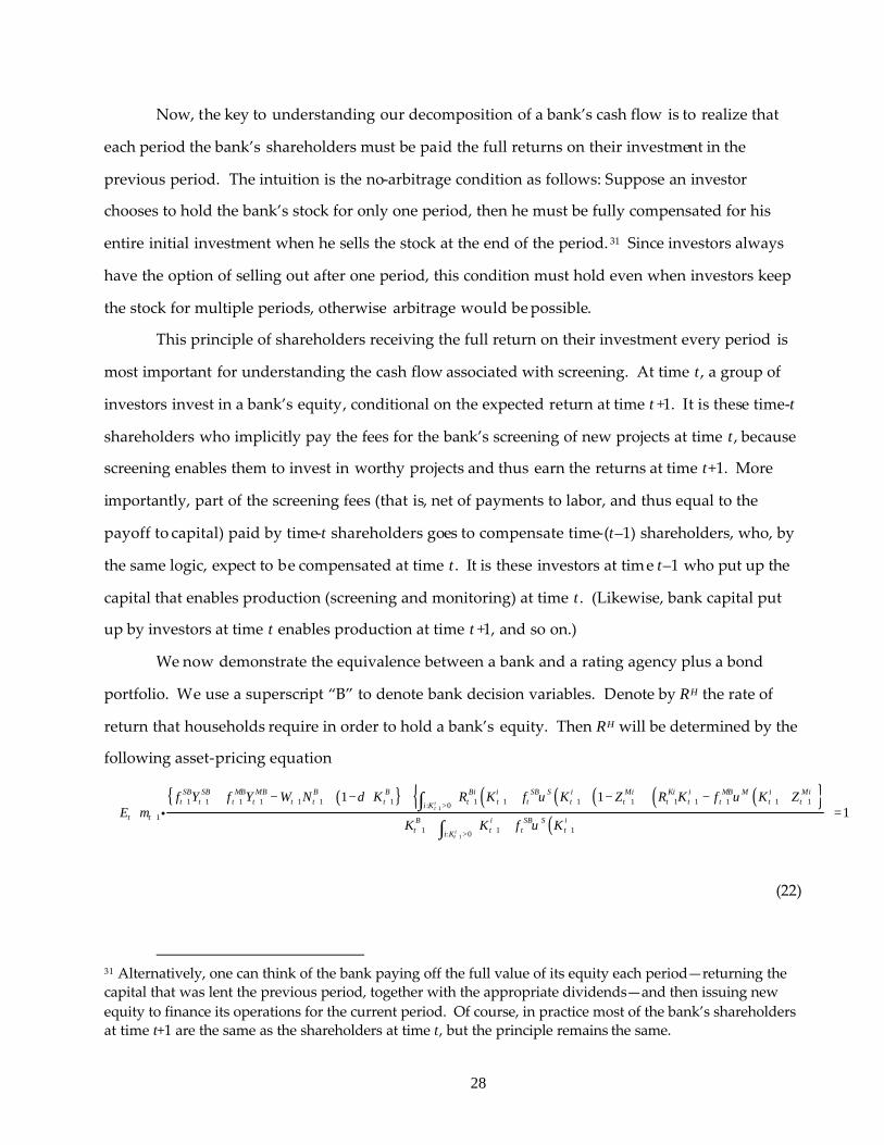
The numerator equals the bank’s total cash flow in period t+1. It is organized into two parts (in

braces {}) to correspond to the cash flows of the two hypothetical divisions, in order to facilitate the

comparison of a bank with a rating agency plus a bond portfolio. The first part is the cash flow of

the service division, which does all the screening and monitoring; every term there is defined

similarly to its counterpart in the numerator of (18)—the cash flow for the rating agency. The

second part is the cash flow of the loan division, equal to the interest income, summed over all the

entrepreneurs to whom the bank has made loans, net of the monitoring costs. Every term is

defined similarly to its counterpart in (21), which is the return on a diversified portfolio of many

bonds, each of which has a payoff similar to the numerator of (20).

The denominator of (22) is the sum of bank capital—comprising the amount the bank uses

for screening and monitoring (KB), the amount it lends to entrepreneurs, and the screening fees put

up by this period’s shareholders—best conceptualized as a form of intangible capital.32

Note that, in order to derive the respective cash flows of the two divisions in the

numerator, we deliberately add monitoring income YMB to the first term and subtract monitoring

costs MB M Mif Zυ∫ from the second. But this manipulation on net leaves the bank’s overall cash

flow unchanged, because

( )1

1 1 1 1: 0it

MB MB M i Mit t t ti K

Y f K Zυ+

+ + + +> = ∫ . (23)

The reason is that the monitoring services produced generate income for the service division, and

those are exactly the services the loan division must buy in order to collect from defaulting

borrowers.

We have so far accounted for all of the cash inflow and outflow of the loan division and the

cash inflow corresponding to the provision of monitoring services for the service division. The

next component is the cash inflow from providing screening services by the service division.

According to the logic of fully compensating shareholders every period (discussed earlier), these

screening services are implicitly paid for by time-t+1 shareholders, and the fees constitute part of

time-t shareholders’ return. They are the analogue of the screening fees in the denominator, which

32 That is, even though not recorded on balance sheets, the screening fees are nonetheless part of the overall investment funded by these investors today, and these investors expect to benefit from the payoff on that investment in the subsequent period.

30

amount to SB SBt tf Y (for a reason similar to (23)), and were paid by time-t shareholders to

compensate time-(t–1) shareholders. The final component of the capital return for the service

division is the return of the depreciated capital to shareholders. (Depreciated capital is in the

capital return of the loan division implicitly since we use gross rates of return in that part of the

numerator.)

C. Equilibrium with Asymmetric Information

The general equilibrium of the model requires the following conditions: (i) Households

optimally choose their consumption, labor supply, holdings of bonds, and holdings of equity in

banks and rating agencies; (ii) Firms in the second period of their existence hire labor optimally

and pay the prevailing wage; (iii) Firms in the first period of their existence choose capital

investment optimally, given the prevailing interest rates; (iv) Banks and rating agencies hire the

optimal amount of labor and produce the optimal amounts of screening and monitoring services,

given that those services are priced at marginal cost; (v) Banks lend capital to firms at the optimal

interest rate, given the riskiness of each firm and the rate of return that households require on bank

loans; (vi) Entrepreneurs in the second period of their lives who are not bankrupt pay off their

loans/bonds and then consume the remaining income from their projects, whereas those who are

bankrupt transfer the output and residual assets of their projects to their creditors; (vii) The sum of

labor demand by banks, agencies, and firms equals the supply by households; and (viii) The sum

of capital demand by banks, agencies, and bond-issuing firms equals the supply by households.

We do not solve explicitly for the full set of equilibrium outcomes for all the variables because we

need only a subset of the equilibrium conditions to make the important points regarding bank

output measurement. A major use of general equilibrium in our model is that it allows us to derive

asset prices (and risk premia) endogenously in terms of the real variables (in particular, the

marginal utility of consumption). Thus, in the context of this model, it is clear where everything

“comes from” in the environment facing banks.

The first step toward proving the nature of the equilibrium is to note that the cash flow of

any bank can be thought of as coming from two assets that households can choose to hold

separately, each corresponding to equity claims on just one division of the bank. Recall that for the

31

purpose of valuing an asset, it is immaterial whether or not the asset actually exists. (See footnote

12.) Thus, it is immaterial whether the bank actually sells separate claims on the different streams

of cash flows coming from its different operations; no bank does. But investors will still value the

overall bank as the sum of two separate cash flows, each discounted by its own risk-based required

rate of return. To take an analogy, Ford’s shareholders in the United States certainly make

different forecasts for the earnings of its Jaguar, Volvo, and domestic divisions and know that

exchange-rate risk applies to earnings from the first two, but not to the third. Shareholders then

add these individual discounted components to arrive at their valuation of the entire company.

It is important to note that no asset-pricing theory implies a unique way to split up a

banks’—or, indeed, any firm’s—cash flow, generated by its various operations. Investors can

choose to think of a bank as comprising the sum of any combination of its operations that adds up

to the entire bank’s cash flow. The crucial point is that the asset-pricing equation (4) must apply to

any and all subsets of a bank’s overall cash flow. Therefore, while it is true that investors can view

a bank as a combination of the service and the loan divisions, im plying that equations (24) and (25)

below must both hold, investors could also divide a bank in many other ways, leading to many

other asset-pricing equations. But we argue that the service vs. loan division is the most

meaningful way of partitioning a bank’s operations for the purpose of understanding real bank

output, because it separates the bank’s production of real output from its holding of assets on

behalf of its investors. Moreover, this division generates two entities that both have real-world

counterparts (that is, rating agencies and bond markets). Therefore, this division is the most useful

both for understanding and for measuring bank output. (See our discussion of measurement

below.)

The asset-pricing equation for valuing the equity of just the service division is:

( )1 1 1 1 1 1 11

1

11.

SB SB MB MB B Bt t t t t t t

t t Bt

f Y f Y W N KE m

Kδ+ + + + + + +

++

+ − + −=

i (24)

The denominator is 1BtK + , since it is the capital used in screening and monitoring. The numerator is

the same as the terms in the first curly bracket in (22), discussed extensively above.

The equation for valuing the equity of just the loan division thus is:

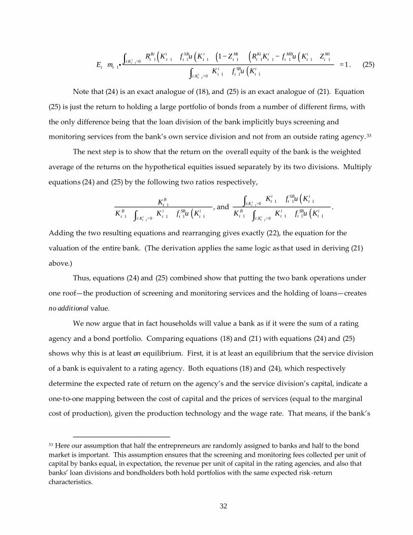
32

( )( ) ( ) ( )( )( )

1

1

1 1 1 1 1 1 1 1 1 1: 01

1 1 1: 0

11

it

it

Bi i SB i Mi Ki i MB i Mit t t t t t t t t ti K

t t i SB it t ti K

R K f K Z R K f K ZE m

K f K

υ υ

υ+

+

+ + + + + + + + + +>+

+ + +>

+ − + − = +

∫∫

i . (25)

Note that (24) is an exact analogue of (18), and (25) is an exact analogue of (21). Equation

(25) is just the return to holding a large portfolio of bonds from a number of different firms, with

the only difference being that the loan division of the bank implicitly buys screening and

monitoring services from the bank’s own service division and not from an outside rating agency.33

The next step is to show that the return on the overall equity of the bank is the weighted

average of the returns on the hypothetical equities issued separately by its two divisions. Multiply

equations (24) and (25) by the following two ratios respectively,

( )1

1

1 1 1 1: 0it

Bt

B i SB it t t ti K

KK K f Kυ

+

+

+ + + +> + + ∫

, and ( )

( )1

1

1 1 1: 0

1 1 1 1: 0

it

it

i SB it t ti K

B i SB it t t ti K

K f K

K K f K

υ

υ+

+

+ + +>

+ + + +>

+ + +

∫∫

.

Adding the two resulting equations and rearranging gives exactly (22), the equation for the

valuation of the entire bank. (The derivation applies the same logic as that used in deriving (21)

above.)

Thus, equations (24) and (25) combined show that putting the two bank operations under

one roof—the production of screening and monitoring services and the holding of loans—creates

no additional value.

We now argue that in fact households will value a bank as if it were the sum of a rating

agency and a bond portfolio. Comparing equations (18) and (21) with equations (24) and (25)

shows why this is at least an equilibrium. First, it is at least an equilibrium that the service division

of a bank is equivalent to a rating agency. Both equations (18) and (24), which respectively

determine the expected rate of return on the agency’s and the service division’s capital, indicate a

one-to-one mapping between the cost of capital and the prices of services (equal to the marginal

cost of production), given the production technology and the wage rate. That means, if the bank’s

33 Here our assumption that half the entrepreneurs are randomly assigned to banks and half to the bond market is important. This assumption ensures that the screening and monitoring fees collected per unit of capital by banks equal, in expectation, the revenue per unit of capital in the rating agencies, and also that banks’ loan divisions and bondholders both hold portfolios with the same expected risk -return characteristics.

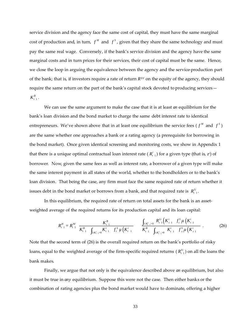
33

service division and the agency face the same cost of capital, they must have the same marginal

cost of production and, in turn, Mf and Sf , given that they share the same technology and must

pay the same real wage. Conversely, if the bank’s service division and the agency have the same

marginal costs and in turn prices for their services, their cost of capital must be the same. Hence,

we close the loop in arguing the equivalence between the agency and the service-production part

of the bank; that is, if investors require a rate of return RSV on the equity of the agency, they should

require the same return on the part of the bank’s capital stock devoted to producing services—

1BtK + .

We can use the same argument to make the case that it is at least an equilibrium for the

bank’s loan division and the bond market to charge the same debt interest rate to identical

entrepreneurs. We’ve shown above that in at least one equilibrium the service fees ( Mf and Sf )

are the same whether one approaches a bank or a rating agency (a prerequisite for borrowing in

the bond market). Once given identical screening and monitoring costs, we show in Appendix 1

that there is a unique optimal contractual loan interest rate ( 1itR + ) for a given type (that is, zi) of

borrower. Now, given the same fees as well as interest rate, a borrower of a given type will make

the same interest payment in all states of the world, whether to the bondholders or to the bank’s

loan division. That being the case, any firm must face the same required rate of return whether it

issues debt in the bond market or borrows from a bank, and that required rate is 1LitR + .

In this equilibrium, the required rate of return on total assets for the bank is an asset-

weighted average of the required returns for its production capital and its loan capital:

( )( )( )( )

1

1 1

1 1 1 1: 011 1

1 1 1 1 1 1 1 1: 0 : 0

.it

i it t

Li i S iB t t t ti KH SV t

t t B i S i B i S it t t t t t t ti K i K

R K f KKR R

K K f K K K f K

υ

υ υ+

+ +

+ + + +>++ +

+ + + + + + + +> >

+ = + + + + +

∫∫ ∫

(26)

Note that the second term of (26) is the overall required return on the bank’s portfolio of risky

loans, equal to the weighted average of the firm-specific required returns ( 1LitR + ) on all the loans the

bank makes.

Finally, we argue that not only is the equivalence described above an equilibrium, but also

it must be true in any equilibrium. Suppose this were not the case. Then either banks or the

combination of rating agencies plus the bond market would have to dominate, offering a higher

34

rate of return for any given level of systematic risk. It is easy to show that neither of the two

possibilities can be true. If either banks could dominate rating agencies plus the bond market, or

vice versa, then either group would do so at every level of operation, since there are constant

returns to scale. But then it cannot be an equilibrium at any time for banks to offer the same rate of

return as the weighted average return to investing in rating agencies plus the bond market. But we

have just shown that such an equilibrium exists. Thus, there cannot be equilibria in which the

overall risk-adjusted return to banks exceeds the return to rating agencies plus the bond market, or

vice versa.

In conclusion, in any equilibrium, the service division of the bank must have a required rate

of return on capital of RSV, and each loan that the bank makes must have the same required return,

RLi, as it would have were it made in the bond market.34

D. Banks Are Mutual Funds!

We have presented the essential features of a simple DSGE model with financial

intermediation. The model shows that since banks perform several functions under one roof,

investors view a bank as a collection of assets—a combination of a bond mutual fund (of various

loans) and a stock mutual fund (one that holds the equities of rating agencies). Investors value the

bank by discounting the cash flow from each asset with the relevant risk-adjusted required rate of

return for that asset. But in general all of the cash flows will have some systematic risk, and thus

none of the required rates will be the risk-free interest rate.

In the context of the model, it is clear that proper measurement of nominal and real bank

output requires that we identify the actual services banks provide (and are implicitly compensated

for) and recognize that these services are qualitatively equivalent to the (explicitly priced) services

provided by rating agencies. So, it is logical to treat bank output the same as the explicit output of

those alternative institutions.

34 We have shown that, in any equilibrium that exists, households demand the same rate of return on each division of the bank as the rate on the rating agency and the bond portfolio, respectively. We have not claimed that an equilibrium must exist in this model, or that the equilibrium described above is unique—there may be multiple equilibria, with different asset prices associated with each one.

35

Another benefit of our approach—and a different intuition for its validity—is that the

measure of bank output it implies is invariant to alternative modes of operation in banks. The

prime example is the securitization of loans, which has become increasingly popular in recent

years, where banks originate loans (mostly residential mortgages) and then sell pools of such loans

to outside investors, who hold them as they would bonds. In this case a bank turns itself into a

rating agency, receiving explicit fees for screening (and servicing over the lifetime of the loan

pool). Securitization should not change a reasonable measure of bank output, since banks perform

the same services whether or not a loan is securitized. Our model, which counts service provision

as the only real bank output, indeed will generate the same measure of bank output regardless of

whether loans are securitized. But if one follows SNA93, then a bank that securitizes loans will

appear to have lower output on average, since it will not be credited with the “output” that is

really the transfer of the risk premium to debt-holders. Thus, under SNA93, an economy with

increasing securitization will appear to have declining bank output, even if all allocations and

economic decisions are unchanged.

E. Different Capital Structures for Banks

The above sub-sections of Section II have all assumed that banks are 100 percent equity

financed. This is unusual in that we are used to thinking of banks as being financed by debt (that

is, deposits). But we will show below that the Modigliani-Miller (MM 1958) theorem holds in our

model, so all our previous conclusions are completely unaffected by introducing debt (deposit)

finance. Of course, there is a large literature in corporate finance discussing how differential tax

treatment of debt and equity causes the MM theorem to break down. But we have deliberately

avoided such complications in order to exposit the basic intuition of our approach. Once that

intuition is clear, it will be simple to extend the model to encompass such real-world

complications.

We have an environment where information is symmetric between banks and households,

so there is no need for screening and monitoring when banks raise funds (that is, sell equity

shares) from households. We thus reasonably assume there are no transaction costs of any kind

between banks and households. We also assume that interest payments and dividends receive the

36

same tax treatment. In this setting, banks’ capital structure is irrelevant, in that the required rate of

return on banks’ total assets is the same with or without debt. When banks are leveraged, the

required rates of return on the bank’s debt and equity are determined by the risk of the part of the

cash flow promised, respectively, to the debtholders and the shareholders. Since debtholders have

senior claim on the bank’s cash flow, the ex ante rate of return they require is almost always lower

than the rate required by shareholders. But the rate of return on the bank’s total assets is the

weighted average of the return on debt and equity, and it equals the return on the assets of an

unlevered, that is, all-equity, bank. This result is a simple application of the Modigliani and Miller

(1958) theorem.

Without deposit insurance, bank deposits are liabilities that are qualitatively the same as

firms’ debt. So, the expected payoff to depositors has the same profile as firms’ debt described in

equation (A14), only without the information processing costs. Households’ Euler equation (4)

determines the expected rate of return on deposits. Applying the MM theorem, the expected rate

of return on the bank’s asset portfolio remains the same regardless of its deposit-to-equity ratio.

Hence, it should set the same interest rate on its loans, ceteris paribus. The implication is that all the

above analysis of the imputation of implicit bank service output remains valid even when banks

are funded partly by deposits. We discuss the extension to deposit insurance in Section III.B; this

issue is analyzed in depth in Wang (2003a).

Armed with this overview of the model and the intuition for the key results, the reader is

now equipped to understand the detailed discussion of the model in Appendix 1.35 Alternatively,

a reader more interested in the measurement implications will now be able to understand the

theoretical background for the measurement discussion that follows in Section III.

35 The main issues we address in detail in Appendix 1 are (i) the exact nature of the debt contract for entrepreneurs’ projects (including the contractual interest rate charged) that come out of the banks’ profit maximization decision; and, (ii) the optimal choice of capital and labor for entrepreneurs, given the terms available on the debt contract.

37

III. Implications for Measuring Bank Output and Prices

This model yields one overarching principle for measurement: Focus on the flow of actual

services provided by banks. This principle applies equally to measuring both nominal and real

banking output—and, by implication, to measuring the implicit price deflator for financial

services. Although the details of the formal model (for example, the contracting problem in

Appendix 1) are sometimes complex, the setup and the results are intuitively sensible. We

assumed that financial intermediaries provide screening and monitoring services, which mitigate

asymmetric information problems between potential borrowers and investors. The model then

implies that the SNA93 recommendations for how to measure implicit financial services—as well

as the recent implementation in the NIPA2003 benchmark revisions—generally do not accurately

capture actual service flows. Since screening and monitoring services capture essential aspects of

actual financial market activities, we would want any measure of bank output to be consistent with

them. Hence, the model highlights several conceptual shortcomings of the SNA/NIPA

framework.

Three main issues arise. First, the model shows that the appropriate “reference rate” for

measuring nominal bank lending services must incorporate the borrower’s risk -premium; that is,

the borrower’s risk-premium is not part of bank output. Intuitively, the borrowing firm must pay

that premium regardless of whether the funds flow through a bank. For example, the firm could

in principle issue bonds (after getting certified by a credit rating agency) or issue some equity

directly to households (if the screening/monitoring needs are not too severe; or if a mutual fund

provides the screening/monitoring services to the household for a fee). The return on those risky

assets reflects the capital return to the firm and is income to households.

Second, the model shows that the timing of bank cash flows will often not match the timing

of actual bank service output, since screening is typically done before the loan generates income.

This problem does not necessarily disappear even when the origination fees are explicitly paid up

front (ruled out in the model), since Generally Accepted Accounting Principles (GAAP) often

require banks to artificially smooth these revenues over the lifetime of the loan, thus inadvertently

reinstating the problem.

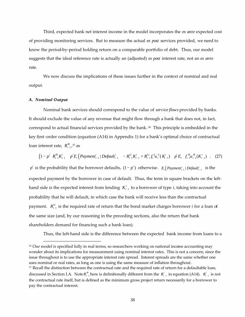
38

Third, expected bank net interest income in the model incorporates the ex ante expected cost

of providing monitoring services. But to measure the actual ex post services provided, we need to

know the period-by-period holding return on a comparable portfolio of debt. Thus, our model

suggests that the ideal reference rate is actually an (adjusted) ex post interest rate, not an ex ante

rate.

We now discuss the implications of these issues further in the context of nominal and real

output.

A. Nominal Output

Nominal bank services should correspond to the value of service flows provided by banks.

It should exclude the value of any revenue that might flow through a bank that does not, in fact,

correspond to actual financial services provided by the bank. 36 This principle is embedded in the

key first -order condition (equation (A14) in Appendix 1) for a bank’s optimal choice of contractual

loan interest rate, 1BitR + ,37 as

( ) ( )1 1 1 1 1 1 1 1 1 1 11 | ( ) ( )i Bi i i i i Li i Li S S i i M M it t t t t t t t t t t t t t tp R K p E Payment Default R K R f K p E f Kυ υ+ + + + + + + + + + +

− + − = + . (27)

ip is the probability that the borrower defaults, (1 )ip− otherwise. ( )1 1|i it t tE Payment Default+ + is the

expected payment by the borrower in case of default. Thus, the term in square brackets on the left-

hand side is the expected interest from lending 1itK + to a borrower of type i, taking into account the

probability that he will default, in which case the bank will receive less than the contractual

payment. 1LitR + is the required rate of return that the bond market charges borrower i for a loan of

the same size (and, by our reasoning in the preceding sections, also the return that bank

shareholders demand for financing such a bank loan).

Thus, the left-hand side is the difference between the expected bank income from loans to a

36 Our model is specified fully in real terms, so researchers working on national income accounting may wonder about its implications for measurement using nominal interest rates. This is not a concern, since the issue throughout is to use the appropriate interest rate spread. Interest spreads are the same whether one uses nominal or real rates, as long as one is using the same measure of inflation throughout. 37 Recall the distinction between the contractual rate and the required rate of return for a defaultable loan, discussed in Section I.A. Note 1

BitR + here is definitionally different from the 1

itR + in equation (A14). 1

itR + is not

the contractual rate itself, but is defined as the minimum gross project return necessarily for a borrower to pay the contractual interest.

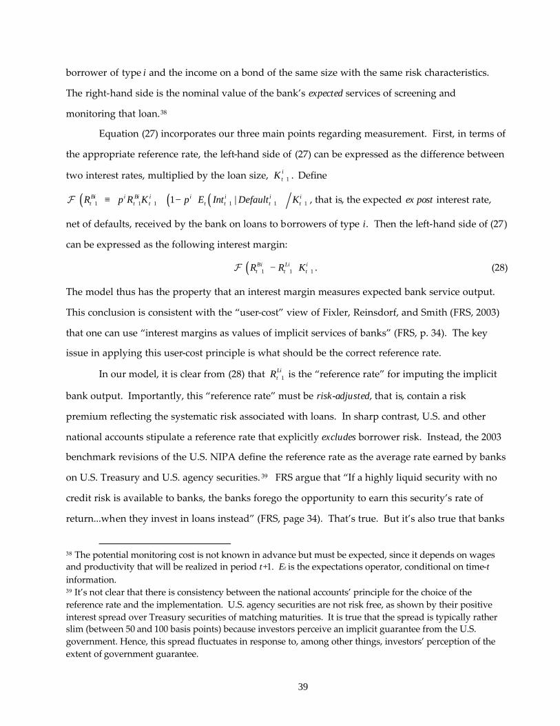
39

borrower of type i and the income on a bond of the same size with the same risk characteristics.

The right-hand side is the nominal value of the bank’s expected services of screening and

monitoring that loan.38

Equation (27) incorporates our three main points regarding measurement. First, in terms of

the appropriate reference rate, the left-hand side of (27) can be expressed as the difference between

two interest rates, multiplied by the loan size, 1itK + . Define

( ) ( ) ( )1 1 1 1 1 11 |Bi i Bi i i i i it t t t t t tR p R K p E Int Default K+ + + + + + ≡ + − F , that is, the expected ex post interest rate,

net of defaults, received by the bank on loans to borrowers of type i. Then the left-hand side of (27)

can be expressed as the following interest margin:

( )1 1 1Bi Li it t tR R K+ + + − F . (28)

The model thus has the property that an interest margin measures expected bank service output.

This conclusion is consistent with the “user-cost” view of Fixler, Reinsdorf, and Smith (FRS, 2003)

that one can use “interest margins as values of implicit services of banks” (FRS, p. 34). The key

issue in applying this user-cost principle is what should be the correct reference rate.

In our model, it is clear from (28) that 1LitR + is the “reference rate” for imputing the implicit

bank output. Importantly, this “reference rate” must be risk-adjusted, that is, contain a risk

premium reflecting the systematic risk associated with loans. In sharp contrast, U.S. and other

national accounts stipulate a reference rate that explicitly excludes borrower risk. Instead, the 2003

benchmark revisions of the U.S. NIPA define the reference rate as the average rate earned by banks

on U.S. Treasury and U.S. agency securities. 39 FRS argue that “If a highly liquid security with no

credit risk is available to banks, the banks forego the opportunity to earn this security’s rate of

return...when they invest in loans instead” (FRS, page 34). That’s true. But it’s also true that banks

38 The potential monitoring cost is not known in advance but must be expected, since it depends on wages and productivity that will be realized in period t+1. Et is the expectations operator, conditional on time-t information. 39 It’s not clear that there is consistency between the national accounts’ principle for the choice of the reference rate and the implementation. U.S. agency securities are not risk free, as shown by their positive interest spread over Treasury securities of matching maturities. It is true that the spread is typically rather slim (between 50 and 100 basis points) because investors perceive an implicit guarantee from the U.S. government. Hence, this spread fluctuates in response to, among other things, investors’ perception of the extent of government guarantee.

40

forego the opportunity to invest in high-risk/high-yielding junk bonds! Thus, in a world with risk,

the opportunity-cost argument alone provides little theoretical guidance in setting the required

rate of return (that is, opportunity cost) of funds, let alone suggesting that one should arbitrarily

define the opportunity cost in terms of a risk -free rate.

Our model clarifies the apparent ambiguity inherent in the “opportunity cost” argument,

by incorporating modern asset pricing theories (the consumption CAPM, specifically). Indeed, by

combining theories of asset pricing and financial intermediation, our model (as well as Wang’s

(2003a, b) partial-equilibrium models that we build upon) can be construed as extending and

generalizing the user-cost framework to take account of uncertainty and asymmetric information.

The central tenet of these asset pricing theories is that an asset’s required rate of return

depends (increasingly) on its systematic risk. In two special cases, the required return equals the

risk-free rate: if there is no systematic risk (that is, only idiosyncratic risk, which creditors can

diversify away) or if investors are risk -neutral. The clear implication is that the correct reference

rate (that is, opportunity cost of funds) for imputing bank lending services should be systematic-

risk-adjusted, except in those special cases. But those cases do not seem to describe the world,

where there are clearly risk premia. Thus, our model makes it clear that the current NIPA

implementation of the user-cost approach—with a risk-free reference rate for lending services—is

unlikely to be appropriate in the realistic world with uncertainty.

To see the intuition for risk-adjusted reference rates, first consider a bank’s point of view.

The loan rate it charges covers both the services it provides and the riskiness of the loan (which

depends on the covariance of the loan’s return with the marginal utility of consumption). In

equilibrium, the loan interest rate, net of implicit service fees, must exactly compensate the

ultimate suppliers of funds (bank shareholders-households in this model) for the risk they bear.

Otherwise, bank shareholders would prefer to hold other assets, for example, bonds or mutual

funds. Conversely, from the borrower’s point of view, he could (at least conceptually) go to a

rating agency and get certified and then borrow from the bond market at the risk -adjusted rate.

After all, virtually no borrowers other than the U.S. government or government agencies can

borrow at the “risk free” rate. Thus, the risk-adjusted rate preserves neutrality with respect to

41

economically-identical institutional arrangements for obtaining external funds; a risk-free rate

would not.40

Securitization further illustrates the rationale for risk -adjusted reference rates. Securitized

loans are now standard in residential mortgages and consumer loans, and are increasingly

common for business lending.41 Under securitization, banks receive explicit payments for their

services, so one measures nominal bank lending output by this service revenue.

Securitization therefore provides a useful conceptual benchmark for indirectly measuring

the implicitly priced output of services in traditional banking. Following the principle of

preserving neutrality among economically -identical lending arrangements, real bank output

should be invariant whether loans are securitized or held on banks’ books. Otherwise, measured

bank output will be inconsistent across time as the fraction of securitized loans changes, even if

there is no real economic change. In fact, NIPA’s use of a risk-free reference rate does make the

current measure of bank output inconsistent over time, because firms are increasingly substituting

bonds for bank loans. Our model effectively supplies a roadmap for imputing implicit bank

service output according to the same decision rules as in securitization: decompose total bank

interest income into partial flows with relative risk profiles that match their securitized

counterparts.

Furthermore, the model implies that the NIPAs mismeasure the opportunity cost of banks’

“own funds” (the difference between assets and liabilities). The model derives the measure of

implicit bank service output—interest income net of the required return on funds—with no

restrictions on a bank’s capital structure. Hence, its conclusions accord in spirit with SNA93’s

40 A similar inconsistency would arise if one applied SNA93’s recommendations for FISIM to a mutual fund that raised funds from investors and bought equity stakes in firms. The SNA93 banking method implies that the nominal output of the mutual fund is the difference between the return on the fund’s portfolio and the potential return were the funds invested in Treasury securities. This clearly seems inappropriate. Indeed, suppose the mutual fund did nothing more than basic bookkeeping and so the fund shareholders were indifferent between owning shares in the fund and owning the underlying firms’ stocks directly. Then the fund’s existence should not alter the underlying firms’ output. But the SNA93 method would count the return due to equities’ risk premium as part of the mutual fund’s output––in turn part of intermediate services purchased by the underlying firms––not as part of the firms’ cost of capital and in turn value added. That is, mutual funds’ output rises at the expense of those firms whose equities they own. 41 By the end of 2003, over 80 percent of residential mortgage loans were sold on the secondary markets and 30 percent of consumer credit were securitized (Flow of Funds, Federal Reserve Board).

42

recommendation that the opportunity cost of a bank’s own funds be netted out of its imputed

service output. But the 2003 NIPA revision explicitly uses the risk-free rate as the user cost of

banks’ own funds. (See FRS, page 36.) The model makes clear that the opportunity cost of funds

for a loan should be risk-adjusted according to the same asset pricing theories whether the lending

is financed by “intermediation” (deposit taking) or by banks’ “own funds.”

Counting the risk premium as part of bank output also overstates GDP. In the model, GDP

is not mismeasured since financial services to the borrowing non-financial firms are an

intermediate input. An SNA93-based measure would just misallocate some part of firms’ value

added to banks. But the logic of the model obviously also applies to loans to households (for

example, mortgages and credit cards), since they also involve risk and require similar risk -

assessment services. Thus, to avoid overstating GDP, we should not incorporate the risk premium

into the consumption of financial services by the household sector.

The second general issue concerning the measurement of bank output highlighted by

equation (27) is the timing mismatch between the cash inflow and the provision of screening

services. In the model, banks screen potential borrowers in period t, but these services are not

compensated until period t+1. As a result, the bank demands a repayment of 1 1( )Li S S it t t tR f Kυ+ + for its

screening services, and this amount exceeds its nominal expenditure on services ( 1( )S S it t tf Kυ + ) by

the gross interest margin. Ideally, one would attribute the value of these services to period t rather

than period t+1.42 To get the timing right, we must attribute the services to the period when the

screening takes place—that is, when the bank originates the loans.

In principle, if banks charge explicit origination fees upfront—rather than rolling these fees

into the interest rate—then the timing mismatch becomes less important. Indeed, firms in practice

often do pay some explicit origination fee when borrowing from banks. However, GAAP

accounting requires that banks amortize the origination fee over the life of a loan instead of fully

recognizing the entire fee as revenue in the period it is generated. So the reported income stream

is artificially smoothed and does not coincide with the actual timing of the production. As a result,

depending on how variable the true screening services are from period to period, nominal bank

42 On the borrowing side, we may think of the screening fee as a cost firms must pay when they purchase and install capital goods in advance, well before the capital begins producing output.

43

output measured based on accounting data may bear little relation to the true output in that

particular period. Hence, accounting data must be used with care to ensure correct timing.

The third general point illuminated by equation (27) is that actual monitoring output differs

from expected monitoring output (that is, 1 1 1( )i M M it t t tp E f Kυ+ + + on the right-hand side of (27)), the

cost of which is incorporated into the expected interest margin (that is, the left-hand side of (27)).

That is, the contractual rate covers expected monitoring services based on the ex ante probability of

default, but monitoring takes place only when a borrower actually defaults ex post. So actual

services rendered differ from expected.

Note that this problem of mismeasuring monitoring services is not simply that the ex ante

interest margin does not equal the ex post interest margin. Instead, neither ex ante nor ex post

interest margin matches the actual services. Broadly speaking, under the still-common banking

practice of charging for services implicitly, we suspect that in good times, banks do less monitoring

than expected while enjoying higher-than-expected interest margins; in bad times, they do more

monitoring than expected while suffering lower-than-expected interest margins. Thus, in a boom,

ex post interest margins exceed the value of banks’ actual service flows. In a recession, ex post

interest margins fall short of the actual value of service flows. (See Appendix 2 for more detailed

technical derivation of this outcome.)

Thus, accurate measurement of the nominal value of bank services requires that we adjust

the ex post interest margin for the actual rate of default. Given considerable data on bank costs,

such adjustments can, in fact, be implemented. For example, using bank holding company data,

Wang (2003b) adjusts the ex post interest income for the realization of defaults to reduce the gap

between imputed and actual output.43

Note also that even when one averages over a large number of loans, the realized

monitoring output is likely to differ from the expected, since the bank cannot diversify away

aggregate risk. This non-diversifiable deviation of actual from expected cash flow is negatively

correlated with shareholders’ marginal utility of consumption, which is precisely the reason why

there is a risk premium incorporated into returns on banks’ loans. That is, in good times, when

43 Going forward, more relevant data are likely to be generated in the coming implementation of the Basel II accord for capital requirement, which encourages banks to develop internal risk management systems.

44

output and consumption are high and so marginal utilities are low, banks generate a lot of residual

cash flow that accrues to shareholders; in bad times, when output and consumption are low, banks

generate less residual cash flow.

We conclude this section by discussing how to extend the model to measure bank depositor

services (for example, direct transaction and payment services, safe deposit boxes, trust services,

etc.). They are not formally analyzed in the model because, conceptually, they raise fewer

complications than lending services, especially regarding the treatment of risk. A straightforward

application of the model yields the same output measure as that in the national accounts—nominal

depositor services equal to the margin between the interest paid and the interest imputed based on

a risk-free reference rate. This is because, without the service component, deposits are simply

fixed-income securities. Given deposit insurance in the United States and elsewhere, the expected

rate of return on the funds in deposit accounts should just be the risk-free rate for all the balances

covered by the insurance. For those balances not covered or without deposit insurance, however,

depositors would demand a higher expected return on their debt stake in the bank. That rate

depends on the default risk of a bank’s asset portfolio and its capital structure. In other words, the

risk-free reference rate for deposits is appropriate only if there is deposit insurance. The same

measure is unlikely to remain correct for countries without deposit insurance, such as New

Zealand.

B. Is Risk Assumption a Service?

In our model, the services that banks produce with their capital and labor are screening and

monitoring loans. One interpretation of NIPA conventions, however, is that they construe this risk

bearing as an additional service provided by banks.44 Although such services are not in our model,

one can, as a matter of accounting, presumably write down many complete, internally consistent

accounting systems that are consistent with any given economic model. Thus, we propose an

accounting system where the provision of risk bearing is not treated as a service. But one can

44 For example, Fixler, Reinsdorf, and Smith (2003) say that “The spread between the reference rate of return and the lending rate is the implicit price that the bank receives for providing financial services to borrowers, which includes the cost of bearing risk”.

45

perhaps also write down another accounting system, also internally consistent, where the

provision of risk-bearing is treated as service output in all transactions. 45

Nevertheless, at least two intuitive criteria help in choosing between different, internally -

consistent accounting frameworks. First, one wants to choose an accounting framework where the

quantities measured have natural economic interpretation. Second, the framework should treat

identical market transactions identically. The system we propose meets these two criteria. The

current system, in contrast, does not.

We’ve already discussed several examples that illustrate these criteria. For example, if

firms are indifferent between borrowing from banks or from the bond market, then we would

want to treat them identically with respect to their marginal decisions. The current national

accounts do not do so.

More generally, the current system does not treat “risk -bearing” consistently across

alternative market arrangements. Indeed, the current accounting system leads to very peculiar

outcomes when applied outside banks narrowly defined. Consider mutual funds. The account

holders of mutual funds are owners of the assets—shareholders. Since the current system credits

bank shareholders with the premium for assum ing risk, mutual fund shareholders should be

treated in the same way. Thus, the NIPA framework would seem to imply that the mutual fund

industry should be credited with producing services equal to actual asset returns in excess of the

risk-free return (multiplied by the market value of the assets).

We do not think it is appropriate to credit the mutual fund industry with producing

trillions of dollars of value added corresponding to the difference between average stock returns

and risk-free interest rates. Our framework would say that we should credit mutual funds only

with providing the services that people think they are buying from mutual funds—transactions

and book-keeping services, and sometimes stock-picking talent as well as more general financial

advice. We think this corresponds much more closely to the economic reality.

Finally, counting risk assumption services as output of the bank causes serious conceptual

difficulties when using the resulting measure of output for productivity studies. Suppose we have

45 We are not aware of any fully-worked-out models that explore the full implications of treating risk assumption as a service output.

46

two banks, one that turns down very risky loans, and one that actively seeks out high-risk projects

and lends to them at high interest rates. Suppose that both banks provide exactly the same

processing services, such as screening and monitoring, and so have the same output by our

definition. It seems undesirable to say that the bank that makes more risky loans—which the other

bank could have made but declined to make—is in fact the more productive bank, solely because of

the riskiness of its loan portfolio.

C. Real Output

The model aims to measure real output as the actual service flow provided by the banking

system. To focus on the issue of risk in bank output measurement, the model considers just bank

lending activities, which essentially involve processing information—specifically financial and

credit data. These services are qualitatively similar to other information services such as

accounting and consulting.

In the model, banks provide two real service outputs: screening and monitoring. Screening

output depends on the number of new loans issued, not the number of outstanding loans. In

contrast, monitoring output depends on the number of outstanding loans (in the model, inherited

from last period). Importantly, the model recognizes that screening and monitoring are

heterogeneous activities, since factors along multiple dimensions affect the risk of a loan and in

turn the procedure and amount of effort needed to evaluate it.46 The model represents those

factors by the single attribute of loan size. In a sense, those factors can be thought of as

determinants of the “quality” and thus affect relative prices (assumed to equal marginal cost) of

various lending services. These relative prices then serve as the weights for computing total

screening (monitoring) output, which should be defined as a Divisia or chain-linked aggregate of

the amount of screening (monitoring) done for different classes of loans.

Measuring the real value of monitoring services presents the same difficulty as that which

affects the nominal value measurement: Measured output (assuming both the risk premium and

46 For example, a loan’s denomination, the borrower’s industry and geographic location, as well as her previous interaction with the bank are all relevant factors. In practice, such risk-driven heterogeneities in screening and monitoring are most pronounced for C&I loans and less so for securitized residential mortgage and consumer loans.

47

the cost of screening are properly accounted for) generally differs from both the actual and the

expected value of monitoring. As noted above, ex post interest margins tend to overstate the actual

amount of monitoring done in good times, and understate in bad times. If we derived the real

value by simply deflating the ex post interest margin by a reasonable proxy for the price of

monitoring (for example, from some estimates of the (marginal) costs associated with a bankruptcy

of a particular size), then measured real output would be similarly biased.

We particularly note one implication of the potential bias in the monitoring output imputed

using realized interest margins. In a downturn, productivity analysts would see a banking sector

experiencing lower imputed output than the norm despite absorbing as much (if not more)

primary or intermediate inputs. Thus, measured banking total factor productivity (TFP) would fall

sharply in a downturn, even if actual TFP did not change.

One way to overcome this difficulty is to measure real monitoring services using direct

indicators. For instance, one can make use of the number of loans overdue or delinquent in each

period to gauge the actual amount of monitoring done; one may be able to collect data on the

associated costs of restructuring and foreclosure to estimate the relative prices of monitoring

different loans.

How do these conceptual issues relate to what the national accounts actually measure (or

try to measure)? The national accounts base their estimates of real output on a real index of

banking services calculated by the Bureau of Labor Statistics (BLS). In terms of lending activities,

BLS (Technical Note 1998) explains that the BLS tries to measure activities such as the number of

loans of various types (commercial, residential, credit card, and so forth). Within these categories,

different loans are weighted by interest rates, the presumption being that loans that bear a higher

interest rate involve more real services. Across categories of services, output is then aggregated

using employment weights.

As the BLS technical note makes clear, limitations on the availability of appropriate data

force many of their choices. Conceptually, at least, we highlight a few of the issues suggested by

the model.

First, one clearly should try to distinguish new loans (which involve screening services)

from the stock of old loans. Second, interest rates are probably not the right weights to use within

48

each loan category. Relative interest rates include the compensation for (i) systematic risk, (ii)

screening services, and (iii) expected monitoring services (tied to expected default probability).

Thus, the relative-interest -rate weights are probably correlated with the proper weights, but

imperfectly. Ideally, one would also try to separate the screening from the monitoring services,

since the timing of undertaking the services differs. Third, in terms of weights across categories,

employment weights can probably be improved on by considering all costs—capital as well as

labor. Last, as noted above, one probably should try to measure real monitoring output more

directly. Even using the number of outstanding loans—as the BLS does, on the grounds that

existing as well as new loans require some services—will not capture the likely counter-cyclical

pattern of actual monitoring services. (In fact, the number of outstanding loans is more likely to be

pro-cyclical.)

D. Price Deflators for Bank Output

Conceptually, what do we mean by the “price” of financial services? We use what seems to

be a natural definition of the price deflator: the nominal value divided by the real quantity index.

This definition has the expected property that the (index of the) quantity of financial services times

the deflator for financial services yields the nominal value of these services. Therefore, having

already discussed both nominal and real measures, we have implicitly discussed how to derive an

appropriate price deflator for banking services.

It’s important to note that our definition, although natural and intuitive, does not

correspond to the way the term “financial market prices” is often used. The interest rate itself (or

an interest rate spread) is often referred to as a price. For example, one might say “the interest rate

is the price of money,” or speak of banks setting an appropriate interest rate as “pricing a loan.”

Similarly, the user-cost literature refers to the interest rate spread between the lending rate and a

reference rate as the “user-cost price” of an asset.

This sometimes loose way of discussing financial market “prices” is appropriate in certain

contexts. But the model makes clear that the interest rate itself, or the interest rate spread, is not

the price for financial services per se, even when the cost of the services is embedded indirectly in

the loan interest rate (or spread). For the same reason, the book value of loans is not the right

49

quantity measure of lending services. (This highlights a conceptual problem with micro studies of

bank cost or profit efficiencies that treat loans’ book value as the quantity of bank output and

interest rate as the price.) Besides, the interest rate also contains the risk premium, which is not

even part of nominal bank services. Hence, in terms of standard national accounting conventions,

it would be inappropriate and unorthodox to refer to the interest rate itself or the interest rate

spread as the price of the financial services.

As an explicit example, consider depositor services. Depositors pay implicitly for the

services they receive by accepting a lower interest rate. Suppose a depositor decides to move his

deposits from a conventional bank to an Internet bank because the latter offers a higher interest

rate. Quite naturally, we would describe this situation as one in which the depositor has decided

to purchase fewer financial services; that is, the nominal quantity of services falls because the real

quantity of services falls. It would clearly be mistaken from the point of view of measuring the

price of financial services to refer to this as a situation in which nominal output falls because the

price (that is, the interest rate spread) falls while the quantity stays fixed.

As an alternative to using interest rates, the general price deflator is often used to deflate

financial output, as in many micro efficiency studies of banks. The model shows that this is not

generally appropriate since the price of financial services output relative to final output need not

be constant. As in any model with multiple sectors, the relative price of two competitive sectors

will not be constant unless the sectors have the same rate of technological change, face the same

factor prices, and have the same factor shares. Since these conditions are probably not true in

general in the world, we have not imposed them in our model. Thus, the relative price of financial

services may change over time.

In summary, the model implies the proper price of financial services by providing

theoretical guidance for measuring the nominal and real values of such services. As importantly,

we now discuss how to meet the practical challenges of implementing the model’s implied

nominal and real output measures.

50

E. Implementing the Model’s Recommendations in Practice

The main steps involve drawing on information available from existing financial market

securities as well as from the measurement that banks already undertake of their own activities

(and the risks associated with those activities). Indeed, Basel II requires that banks assess their

risks even more carefully than they already do—offering an opportunity for improving national

accounts measures.

To measure the value of nominal bank services properly, we must first estimate the risk

premium on bank loans, since that is not part of bank financial services and should be removed

from total interest margin. The risk premium on comparable market securities (for example,

commercial paper and certain corporate bonds), which are subject to the same systematic risk,

serves as a good proxy. Such proxies are readily available, given the depth and breadth of fixed-

income securities markets. Wang (2003b) suggests some securities one may use, and indeed,

provides a preliminary estimate of bank service output free of the risk-premium. (Her estimate

suggests that on average, the risk premium may amount to 20 to 25 percent of imputed bank

service output.)

Second, we need the timing of measuring output—screening in particular—to match the

timing of rendering of the services rather than the timing of revenue generation from the services.

National accountants can collect cash-based accounting data on total origination income, and then

estimate the true screening output by deflating the income with explicit origination fees, which

also serve as proxies for similar charges that are implicit.47 Or national accounts can use direct

indicators, such as total number of new loans made, with the number of new loans in each loan

category weighted by the mean origination fee for that category.

Third, to address the issue that actual monitoring services (both nominal and real) are

47 Demand-side factors may also affect the relative price of lending services. They are tied to the definition of markets, as well as to the degree and form of competition in a market. The scope of a lending market is likely to differ across classes of loans. Making C&I loans to large corporations is likely to be a national market, whereas lending to medium and especially small companies is more localized and thus poses the greatest challenge to the construction of an aggregate price index. Indeed, banks have chosen to specialize in lending to such companies in response to continuing encroachment from the commercial paper and bond markets.

51

likely to differ from both their expected and measured values, one can make use of bank data on

actual loan default rates, as noted above. Alternatively, since the correct reference rate equals the

rate of return on market securities (for example, commercial paper) with risk-return characteristics

comparable to those of bank loans, one may use ex ante and ex post returns on such “matched”

fixed-income market securities to infer bank service flows.

Measuring real services raises the further issue of how to weight various screening and

monitoring activities, given cross-category differences in costs. A carefully designed survey of

banks should provide information on how the characteristics of loans (for example, size, type, etc.)

and borrowers (for example, past credit history with the lending bank) affect processing costs—

both labor and capital. Such information could then indicate how to weight different categories of

lending in constructing an index of the actual financial services rendered.

For example, it seems likely that borrowers’ characteristics have very little impact on the

cost of screening and monitoring securitized real estate and consumer loans, since the process is

rather standardized. Indeed, government-sponsored enterprises (GSEs) such as Fannie Mae

specify a standard set of attributes for (so-called “conforming”) residential mortgages they would

purchase and sell on the secondary markets. Credit scoring systems largely standardize the

origination of auto and credit card loans that are subsequently securitized. Securitization also

standardizes the paperwork involved in servicing—including monitoring—these loans over their

lifetime. These developments imply that originating any conforming mortgage loan can be

reasonably considered a single product, and servicing a securitized mortgage loan is another

product. The same applies to originating or servicing a securitized auto loan or credit card loan.

In contrast , the form and intensity of screening and monitoring most likely vary

substantially across different types of C&I loans. Each screening production function, and to a

lesser extent each monitoring function, probably applies only to a narrowly defined type of loans.

For example, loans corresponding to the same screening function may share such features as

having face values within a certain range (for example, from one to two million dollars), applying

to a specific industry and geographic area, or going to borrowers in good standing with a bank for

a certain length of time (for example, one to two years). So, C&I loans reported within one broad

category will ideally be disaggregated into multiple screening categories.

52

Finally, consider depositor services. It seems easier to define a product for depositor

services than for lending services, since depositor services are more homogeneous, both across

banks and in terms of product characteristics (fewer dimensions). Conceptually, each distinct type

of transaction should be viewed as one depositor service output.48 Each ATM or teller-assisted

transaction is then ideally a composite good of several distinct activities. For practical reasons, we

can define each visit to an ATM or a teller as one unit of a service product, since there is evidence

that each ATM or teller visit is reasonably similar in complexity. Similarly, without data on the

number of each distinct type of transaction, we can treat maintaining each account of a given type

as one product and use the number of deposit accounts of different types to measure output. That

amounts to assuming each account of a given type requires the same amount of bookkeeping,

payment processing, etc., every period. 49

Demand-side factors may be particularly relevant for influencing relative prices across

different types of depositor services. Markets for depositor services have a significant

geographical dimension. Convenience (for example, access to nearby branches and extensive ATM

networks) is a central consideration for consumers when choosing where to establish accounts.

Naturally, the degree and form of competition in a local market influences the relative prices.

More-competitive local markets mean lower prices, ceteris paribus.50 Taking into account the

demand factors can help one estimate relative prices for deriving an index of aggregate depositor

service output.

We conclude this section by noting briefly that financial instruments other than loans, from

which we abstract in the model, raise measurement issues similar to those concerning lending, as

discussed above. Thus, our model’s implication for output measurement applies as well to these

48 For instance, safe deposit box rentals are a homogeneous activity, so are wire transfers, money orders, and cash withdrawals. To a lesser degree, so are cashing a check and opening an account of a specific type. 49 Existing studies use the dollar balance of deposits to measure the output of depositor services, implicitly assuming that the service flow is in proportion to the account balance. But Wang (2003a) has shown that the relationship between the quantity of services and the account balance is likely to be highly non-linear and time-varying. 50 A number of studies find, among other things, that markets with lower concentration or more mobile households seem more competitive. See, for example, Calem and Carlino (1991), Cohen and Mazzeo (2004), and Dick (2003).

53

more exotic financial instruments and so do our recommendations for implementing the output

measure in practice.

IV. Further Implications for Measurement

The general framework of the model is helpful for clarifying several other issues in the

literature on measuring bank output. These include the widespread use of assets and liabilities

themselves as measures of bank output; the question of whether to include capital gains as part of

bank output; and how to measure “other” financial services and instruments provided by banks.

First, the model provides no theoretical support for the widespread practice of using the

dollar value of interest-bearing assets (loans plus market securities) on bank balance sheets

deflated by, for example, the GDP deflator, as real bank output. This practice is standard in the

empirical microeconomic literature on bank cost functions and productivity.51 Our model suggests

a simple counterexample, in the spirit of the bank that does nothing. Suppose a bank has

accumulated a loan portfolio by doing prior screening and monitoring, but originates no new loans

and does not need to monitor any old ones at a particular point in time. Then our model makes it

clear that the bank has zero service output in that period. But the micro literature would conclude

that the bank’s output is arbitrarily large, depending on the size of its existing loan portfolio.

Second, although the model does not explicitly consider capital gains, it provides a guiding

principle for determining whether capital gains should be counted in banking or financial output.

Capital gains and interest income are two often interchangeable ways of receiving asset returns,

with the former related more often to unexpected returns and the latter more often to expected

returns. If interest income is often employed as implicit compensation for financial services

provided without explicit charge, then in principle capital gains can be used in place of interest for

the same purpose. By design, such capital gains will be expected gains, since the service provider

expects to be compensated. These gains should be recognized as implicit compensation for real

financial services. Otherwise, capital gains should not be recognized.

51 See for example, Berger and Mester (1997) and Berger and Humphrey (1997), for surveys of the literature and the approaches commonly used.

54

To illustrate this principle, we use the same example of screening services in lending.

Suppose, instead of holding loans on its balance sheet, a bank sells them after its shareholders have

put up the initial funding, consisting of both the productive capital lent to the firms and the

screening fees. Also, assume that the bank records only the value of the capital lent, but not the

screening fees, as assets on its balance sheet.52 Accordingly, the loans’ contractual interest rates are

quoted with respect to just the capital lent, although the expected value of the interest will cover

the screening fees as well. Then, when the bank sells those loans, that is, debt claims on the firms’

cash flows, it will enjoy a capital gain equal to the value of the screening fees, since the present

value of those claims exceeds the book value by exactly the amount of the fees. Clearly, the capital

gain in this case is qualitatively the same as the extra interest income banks receive in

compensation for their services. So this capital gain should be counted as bank output.

On the other hand, following the same principle, we argue that capital gains or losses

purely due to the random realization of asset returns, that is, unexpected gains or losses, should

not be counted as financial output. This can be seen in the model from the fact that the ideal

reference rate is an ex post rate. The economic intuition is fairly clear, although it is best illustrated

with multi-period debts. Suppose we modify the model so that entrepreneurs and their projects

last three periods. Then firms would borrow two-period debt, which would be screened and

monitored in the usual way. Suppose also that aggregate technology is serially correlated. Then a

favorable realization of technology would lead to a capital gain on all bonds and bank loans that

have yet to mature, since a good technology shock today raises the probability of good technology

in the next period, which reduces the probability of bankruptcy in that period. But these capital

gains do not reflect any provision of bank services—in fact, loans one period from maturity would

be past the screening phase, and would not yet require monitoring—and thus the capital gains

should not be counted as part of output. Intuitively, the only exception to this rule would come if

the capital gains on the loans were due to the provision of some banking service. For example, if

banks provide specialized services to firms that make these firms more productive, leading to an

52 This is a quite likely scenario, since the fees are like intangible assets, which are often poorly or simply not accounted for on balance sheets.

55

appreciation in the value of their assets, one should count some of that gain. This seems unlikely

in the context of banks, but it may be realistic for venture capital firms.

Third, our model and its implied measure of bank output can be readily applied to valuing

implicit services generated by banks when they create financial instruments other than loan

contracts. Our method, therefore, can also be used to measure implicit services generated by other

financial institutions, and these institutions create a wide variety of financial instruments that are

more complex than loans.

The general applicability of our method stems from the fact that a loan (that is, a bond)

subject to default risk is equivalent to a default-free loan combined with a short position in a put

option.53 Denote the contractual interest rate as Ri, and a project’s actual rate of payoff as RK. Then

the payoff on a defaultable loan equals min [Ri, RK]; a lender receives either the promised interest

or the project’s actual payoff, whichever is less. This is because a borrowing firm has only limited

liability: Its owners cannot be forced to pay its losses from their private assets. We can rewrite the

risky loan’s payoff as:

min [Ri, RK] = Ri – max [0, Ri – RK]. (29)

The first term describes the payoff from a riskless loan––guaranteed to pay Ri, while the

second term (max[.]) is exactly the same payoff as a put option on the project with a strike price of

Ri. That is, when the project pays less than Ri, the option holder will exercise the option––sell the

project and receive Ri ––and earn a net return of Ri – RK; when the project pays more than Ri, the

option holder will not exercise the option and thus earn a net return of zero. The negative sign in

front of the second term means the lender of the defaultable loan is shorting (that is, selling to the

borrower) the put option. Equation (29) describes an understanding well-known in corporate

finance, which is that bondholders of a firm in essence write a put option to shareholders of the

firm.

In the case of banks, this means that issuing a loan is qualitatively the same as writing (that

is, holding a short position in) a put option to the borrower. The processing costs incurred should

be the same as well, since all the risk in a defaultable loan lies in the embedded put option. So

53 Put options in general offer the holder the option to sell an asset (real or financial) at a pre-specified price, to the party that wrote (that is, shorted) the option.

56

screening and monitoring is needed only for that risky component, whereas the other

component—the riskless loan—should be virtually costless to process. Therefore, the implicit

services that banks produce in the process of underwriting a loan can be viewed as equivalent to

services generated in the process of creating a financial derivatives contract. This means that the

measure of implicit bank services implied by our model can be applied equally well to similar

services that financial institutions generate in the process of creating other types of financial

instruments. The general principle is the same: apply asset pricing theories to price the financial

instrument by itself; the difference between that value and the security’s actual value yields the

nominal value of the implicit services.

V. Conclusions

In this paper, we develop a dynamic stochastic general equilibrium model to address

thorny issues in the measurement of financial service output. The model focuses on financial

institutions’ role in resolving asymmetric information––performing necessary screening and

monitoring services. We show that understanding the model’s equilibrium conditions for asset

pricing helps resolve some of the perplexing conceptual questions present in the literature. In the

model, measuring real output involves measuring the flow of actual services produced by financial

institutions; measuring nominal output requires measuring the payments that correspond to these

services.

The economic intuition for our main results comes from the fact that one wants to measure

the output of economically similarly institutions the same way. In the model and in the world, the

services that banks provide to borrowers in essence combine the services of a rating agency with

funding through the bond market. But the “bond market” is clearly just a conduit for transferring

funds from households to firms; equally clearly, the return on those funds, including any risk

premium, is not the output of the rating agency! Instead, those funds are properly considered part

of the value added of the borrowing firm (that is, a return on its capital). Analogously, we want to

count the services provided by banks (screening and monitoring) as bank output; but we do not

57

want to include as bank output the risk premium––the part of the cash flow that simply represents

the transfer of capital income from the borrower to the household.

Furthermore, our model and its implied output measure satisfy the intuitive principle that

a firm’s output is invariant with regard to its source of external funding—bond issues or bank

loans in particular—as long as its liabilities have the same risk-return profile and incur the same

amount of informational services. This makes intuitive sense, since the firm would have to pay the

same risk premium and the same service charges (implicit or explicit) no matter whether the funds

flowed through a bank or through the bond market.

The model thus highlights the conceptual shortcoming in the exist ing national accounting

measure of bank output. By counting the risk premium as part of nominal bank output, the

current SNA93 and NIPA measures treat economically identical alternative funding institutions

differently and alter the output of the borrowing firm depending on its source of funding. At the

same time, the model makes clear that the book value of financial assets on banks’ balance sheet,

commonly used as the measure of bank output in the large literature of micro banking studies,

generally does not correspond to the true bank output, nominal or real.

In addition, the model highlights two main practical problems with measuring bank output

accurately. First, the timing of cash flows will often not match the timing of actual bank services,

since actual screening is often done in a period before a loan generates income for its originating

bank. Second, expected bank net interest income in the model incorporates the ex ante expected

cost of providing monitoring services; but ex post, the actual quantity and nominal value of these

services do not match the actual net interest income of the bank. We have discussed how one can

address these shortcomings in the existing measures.

More generally, we advocate a model-based approach to measurement for conceptually

challenging areas of financial services and insurance. 54 In these areas, we suggest that researchers

write down an explicit model of what each firm/industry does, and then base measurement on the

model. Too often researchers focus from the very beginning on what data are available, instead of

asking what data are needed, even in principle, to answer measurement questions fully and

54 For recent studies, see, for example, Schreyer and Stauffer (2003), who consider an extensive set of services provided by financial firms; Triplett and Bosworth (forthcoming, chapter 6) discuss the measurement of insurance output.

58

accurately. Hence, we advocate using the model to clarify what we want to measure, and thus

what the ideal data set is. Only after we know how to do measurement in principle can we begin

to compromise in practice. And if the shadow costs of the data availability constraints are too

high, the measurement community can call for additional data collection projects. To do so, it is

essential that it know what kinds of new data have the highest priority, and why.

Our approach suggests several priorities for extending the theory and collecting data. On

the theory side, our method applies directly to bank services produced in the process of generating

financial instruments other than loans (for example, derivatives). Likewise, our model applies to

the production of financial services by non-bank intermediaries. Thus, our work serves as a

template for measuring financial services output of the financial sector in general. Also, our

method connects the financial measurement literature to the vast amount of research on asset

pricing and corporate finance. Thus, although we have deliberately excluded some real-world

complexities (for example, realistic tax treatment of interest and capital gains), large literatures

work these issues out in detail, and their conclusions can be readily incorporated into our

framework. Some of these issues, such as the effects of deposit insurance, are analyzed in depth in

Wang (2003a).

On data collection, we noted the need to measure the risk profiles of banks’ assets, and

suggested that the reporting requirements of Basel II can generate data useful for this purpose.

Also, constructing an index of real bank output requires better survey data than are now available.

For example, data on how marginal costs of originating and monitoring loans vary with size and

other characteristics would be useful.

We conclude by summarizing the answers that our model implies for the four questions

posed in the Abstract; these questions received detailed treatment in the paper. First, the correct

reference rate must incorporate risk. Second, one does not in fact want to use an ex ante measure of

the risk premium on bank funds in the reference rate—using an ex post holding return on bonds of

comparable riskiness comes closer to measuring the production of actual bank services. But the

timing mismatch and other problems mean that in general no single reference rate provides a

perfect measurement of the nominal value of implicit service output. Third, the price deflator for

financial services is not generally the overall price level. Financial services are a kind of

59

information product, qualitatively similar to other information processing services (for example,

consulting); in general, the price of financial services relative to final output will not be constant.

Fourth, we should count capital gains as part of financial services output only if the return is

implicit compensation for actual services provided.

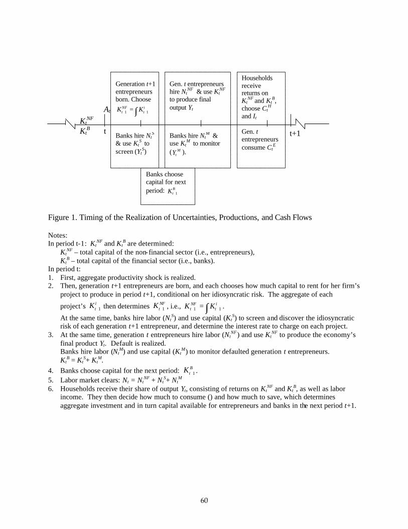
Figure 1. Timing of the Realization of Uncertainties, Productions, and Cash Flows Notes: In period t-1: Kt

NF and KtB are determined:

KtNF – total capital of the non-financial sector (i.e., entrepreneurs),

KtB – total capital of the financial sector (i.e., banks).

In period t: 1. First, aggregate productivity shock is realized. 2. Then, generation t+1 entrepreneurs are born, and each chooses how much capital to rent for her firm’s

project to produce in period t+1, conditional on her idiosyncratic risk. The aggregate of each

project’s 1itK + then determines 1

NFtK + , i.e., 1 1

NF it tK K+ += ∫ .

At the same time, banks hire labor (NtS) and use capital (Kt

S) to screen and discover the idiosyncratic risk of each generation t+1 entrepreneur, and determine the interest rate to charge on each project.

3. At the same time, generation t entrepreneurs hire labor (NtNF) and use Kt

NF to produce the economy’s final product Yt. Default is realized. Banks hire labor (Nt

M) and use capital (KtM) to monitor defaulted generation t entrepreneurs.

KtB = Kt

S+ KtM.

4. Banks choose capital for the next period: 1BtK + .

5. Labor market clears: Nt = NtNF + Nt

S+ NtM

6. Households receive their share of output Yt, consisting of returns on KtNF and Kt

B, as well as labor income. They then decide how much to consume () and how much to save, which determines aggregate investment and in turn capital available for entrepreneurs and banks in the next period t+1.

At

Generation t+1 entrepreneurs born. Choose

1 1NF it tK K+ += ∫

Households receive returns on Kt

NF and KtB,

choose CtH

and It Gen. t entrepreneurs consume Ct

E

t t+1 Kt

NF Kt

B Banks hire NtS

& use KtS to

screen (YtS)

Gen. t entrepreneurs hire Nt

NF & use KtNF

to produce final output Yt

Banks hire NtM &

use KtM to monitor

( MtY ).

Banks choose capital for next period: 1

BtK +

60

Figure 2.A Cash Flows for the Assessment Agency’s Shareholders Who Invest in 1

AtK +

Notes: 7. t: the end of period t ,

t +1: the end of period t +1. 8. Cash inflows are represented by upward arrows, and outflows by downward arrows. 9. The agency’s shareholders invest in 1

AtK + at the end of period t, and 1

AtK + is used in production in

period t+1. 10. From the agency’s operation (i.e., screening generation-t+1 and monitoring generation-t projects), the

shareholders receive a variable profit of 1 1 1 1SA SA MA MA

t t t tf Y f Y+ + + ++ – 1 1A

t tW N+ + .

11. The shareholders invest 1AtI + , and if they were to sell their claims at the end of period t +1, they would

receive 2AtK + . 2

AtK + – 1

AtI + = 1(1 ) A

tKδ +− , i.e., the initial capital net of depreciation. Figure 2.B Cash Flows for Bondholders Who Invest in Generation-t Firm i’s Capital Notes: 1. At the end of period t, bondholders pay for both generation-t firm i’s productive capital 1

itK + and the

associated screening fee 1( )SA S it tf Kυ + .

2. At the end of period t+1, bondholders either receive the contracted interest rate 1itR + , or pay the

necessary monitoring fee ( )1 1MA M i

t tf Kυ+ + and receive all the residual payoff.

1AtI +

1 1A

t tW N+ +

t t+1

1A

tK +

2AtK +

1 1 1 1SA SA MA MA

t t t tf Y f Y+ + + ++

t

1 1( )i SA S it t tK f Kυ+ ++

( )( ) ( )( )( )

1 1 1 1

1 1 1 1 1

1i i SA S i MAit t t t t

Ki i MA M i MAit t t t t

R K f K Z

R K f K Z

υ

υ

+ + + +

+ + + + +

+ −

+ −

t+1

61

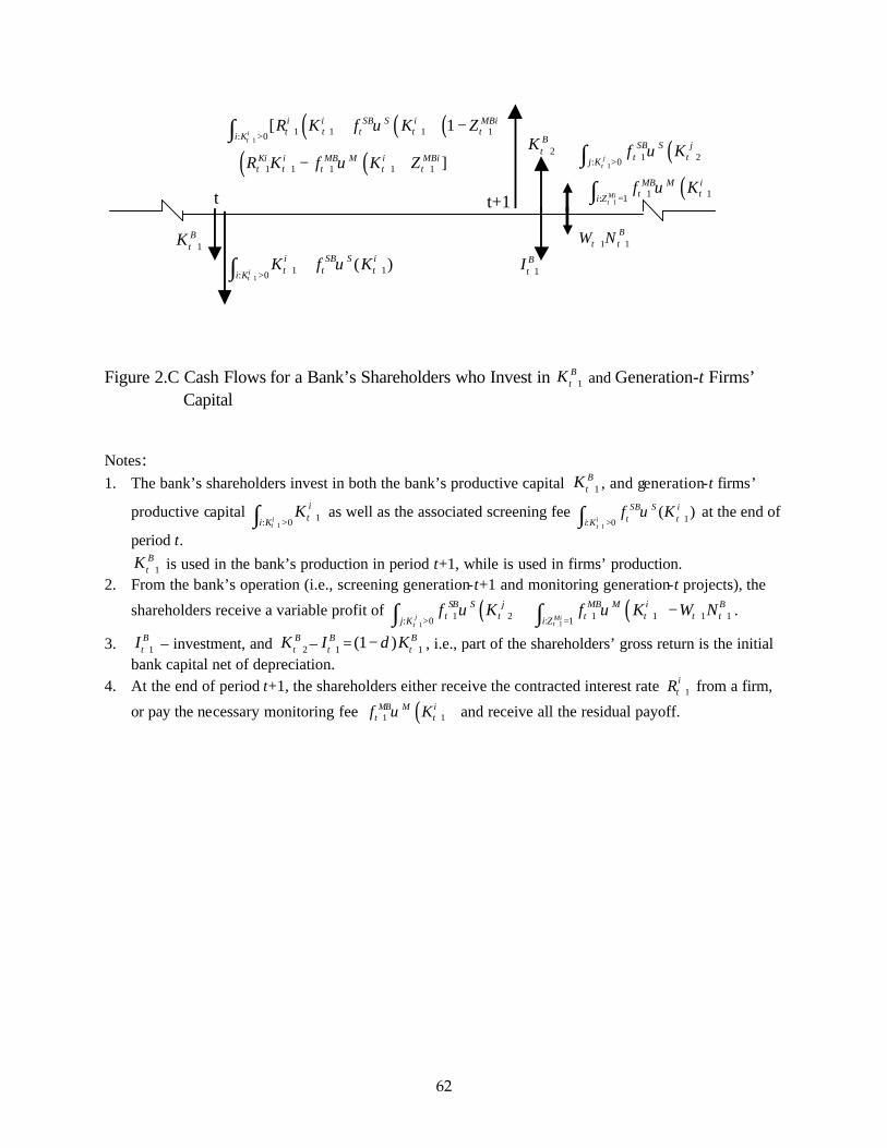
Figure 2.C Cash Flows for a Bank’s Shareholders who Invest in 1

BtK + and Generation-t Firms’

Capital Notes: 1. The bank’s shareholders invest in both the bank’s productive capital 1

BtK + , and generation-t firms’

productive capital 1

1: 0it

iti K

K+

+>∫ as well as the associated screening fee 1

1: 0( )

it

SB S it ti K

f Kυ+

+>∫ at the end of

period t.

1BtK + is used in the bank’s production in period t+1, while is used in firms’ production.

2. From the bank’s operation (i.e., screening generation-t+1 and monitoring generation-t projects), the

shareholders receive a variable profit of ( ) ( )11

1 2 1 1 1 1: 0 : 1j Mitt

SB S j MB M i Bt t t t t tj K i Z

f K f K W Nυ υ++

+ + + + + +> =+ −∫ ∫ .

3. 1BtI + – investment, and 2

BtK + – 1

BtI + = 1(1 ) B

tKδ +− , i.e., part of the shareholders’ gross return is the initial bank capital net of depreciation.

4. At the end of period t+1, the shareholders either receive the contracted interest rate 1itR + from a firm,

or pay the necessary monitoring fee ( )1 1MB M i

t tf Kυ+ + and receive all the residual payoff.

1BtI +

1 1B

t tW N+ +

t

11 1: 0

( )it

i SB S it t ti K

K f Kυ+

+ +>+∫

2BtK + ( )

( )1

1

1 2: 0

1 1: 1

jt

Mit

SB S jt tj K

MB M it ti Z

f K

f K

υ

υ+

+

+ +>

+ +=+

∫∫

t+1

1BtK +

( )( )( )( )( )

11 1 1 1: 0

1 1 1 1 1

[ 1

]

it

i i SB S i MBit t t t ti K

Ki i MB M i MBit t t t t

R K f K Z

R K f K Z

υ

υ

++ + + +>

+ + + + +

+ −

+ −

∫

62

References Akerlof, G. (1970). “The Market for ‘Lemons’: Quality Uncertainty and the Market Mechanism.”

Quarterly Journal of Economics 84(3): 488-500. Allen, Franklin and Anthony M. Santomero. (1997). “The Theory of Financial Intermediation.” Journal

of Banking and Finance 21(11-12): 1461-1485. Allen, Franklin and Anthony M. Santomero. (1999). “What Do Financial Intermediaries Do?” Journal

of Banking and Finance 25(2): 271-294. Basu, Susanto, John G. Fernald, Nicholas Oulton, and Sylaja Srinivasan. (2003). “The Case of the

Missing Productivity Growth: Or, Does Information Technology Explain why Productivity Accelerated in the US but not the UK?” In NBER Macroeconomics Annual 2003, ed. Mark Gertler and Kenneth Rogoff. Cambridge, MA: MIT Press.

Barnett, W. A. (1978). “The User Cost of Money,” Economic Letters 1(2), p. 145-49. Berger, A. N. and D. B. Humphrey. (1997). “Efficiency of Financial Institutions: International Survey

and Directions for Future Research.” European Journal of Operational Research 98(2): 175-212. Berger, A. N. and L. J. Mester. (1997). “Inside the Black Box: What Explains Differences in the

Efficiencies of Financial Institutions?” Journal of Banking and Finance 21(7): 895-947. Bernanke, Ben and Mark Gertler. (1989). "Agency Costs, Net Worth, and Business Fluctuations."

American Economic Review 79(1): 14-31. Bernanke, Ben S., Mark Gertler, and Simon Gilchrist. (1999). “The Financial Accelerator in a

Quantitative Business Cycle Framework.” In Handbook of Macroeconomics,15(1C), eds. Ben S. Bernanke, Mark Gertler, and Simon Gilchrist. New York: Elsevier Science, North-Holland. 1341-1393.

Bureau of Labor Statistics. (1998). “Technical Note on Commercial Banks—SIC 602: Output

Components and Weights.” Manuscript, December. Calem, Paul S. and Gerald A. Carlino. (1991). “The Concentration/Conduct Relationship in Bank

Deposit Markets.” Review of Economics and Statistics 73(2): 268-276. Carlson, Mark and Roberto Perli. (2003). “Profits and Balance Sheet Developments at U.S. Commercial

Banks in 2002.” Federal Reserve Bulletin 89(6): 243-270. Cochrane, John, H. (2001). Asset Pricing. Princeton:Princeton University Press.

63

Cohen, Andrew M. and Michael Mazzeo. (2004). “Market Structure and Competition Among Retail

Depository Institutions.” FEDS Working Paper 2004-04, Federal Reserve Board of Governors. Diamond, D. W. (1984). “Financial Intermediation and Delegated Monitoring.” Review of Economic

Studies 51(3): 393-414. Diamond, D. W. (1991). “Monitoring and Reputation: The Choice between Bank Loans and Privately

Placed Debt.” Journal of Political Economy 99(4): 688-721. Dick, Astrid A. (2003). “Nationwide Branching and its Impact on Market Structure, Quality and Bank

Performance.” FEDS Working Paper 2003-35, Federal Reserve Board of Governors. Also forthcoming in the Journal of Business.

Diewert, W. E. (1974) “Intertemporal Consumer Theory and the Demand for Durables.” Econometrica

42(3): 497-516. Diewert, W. E. (2001), “Measuring the Price and Quantity of Capital Services Under Alternative

Assumptions.” Discussion Paper 01-24, Department of Economics, University of British Columbia. Fixler, D. J. and K. D. Zieschang. (1992). “User Costs, Shadow Prices, and the Real Output of Banks.”

In Studies in Income and Wealth (56), eds. Z. Griliches. NBER. Fixler, D. J., M. B. Reinsdorf, and G. M. Smith. (2003). “Measuring the Services of Commercial Banks

in the NIPAs - Changes in Concepts and Methods.” Survey of Current Business 83(9): 33-44. Fixler, D. J. (2004). “Discussion of the Finance and Insurance Output Measurement.” In Services

Productivity in the United States: New Sources of Economic Growth, eds. Jack. E. Triplett and Barry P. Bosworth. Forthcoming.

Froot, K. A. and J. C. Stein. (1998). “Risk Management, Capital Budgeting and Capital Structure

Policy for Financial Institutions: An Integrated Approach.” Journal of Financial Economics 47(1): 55-82.

Hancock, D. (1985). “The Financial Firm: Production with Monetary and Nonmonetary Goods.” Journal of Political Economy 93(5): 859-880.

Kwark, Noh-Sun. (2002). “Default Risks, Interest Rate Spreads, and Business Cycles: Explaining the

Interest Rate Spread as a Leading Indicator.” Journal of Economic Dynamics and Control 26 (2): 271-302.

64

Leland, H. E. and D. H. Pyle. (1977). “Informational Asymmetries, Financial Structure, and Financial Intermediation.” Journal of Finance 32(2): 371-387.

Modigliani, F. F. and M. H. Miller. (1958). “The Cost of Capital, Corporation Finance, and the Theory of Investment.” American Economic Review (48): 261-297.

Ramakrishnan, R. and A. V. Thakor. (1984). “Information Reliability and A Theory of Financial

Intermediation.” Review of Economic Studies 51(3): 415-432. Schreyer, P. and Stauffer, P. (2003). “Financial Services in National Accounts: Measurement Issues

and Progress.” OECD Task Force on Financial Services in the National Accounts.

System of National Accounts 1993. (1993). Published jointly by the Commission of the European Communities/Eurostat, the International Monetary Fund, the Organization for Economic Co-operation and Development, the Statistics Division of the former Department for Economic and Social Information and Policy Analysis and the regional commissions of the United Nations Secretariat, and the World Bank.

Townsend, R. M. (1979). “Optimal Contracts and Competitive Markets with Costly State

Verification.” Journal of Economic Theory 21(1): 265-293. Triplett, Jack. E. and Barry P. Bosworth. (2004). “Price, Output, and Productivity of Insurance:

Conceptual Issues,” Chapter 6 in Services Productivity in the United States: New Sources of Economic Growth. Brookings Institution Press. Forthcoming.

–––– (2004). “Measuring Banking and Finance: Conceptual Issues.” Chapter 7 in Services Productivity

in the United States: New Sources of Economic Growth. Brookings Institution Press. Forthcoming. Wang, J. C. (2003a). “Loanable Funds, Risk, and Bank Service Output.” Working Paper 03-4, Federal

Reserve Bank of Boston. Wang, J. C. (2003b). “Service Output of Bank Holding Companies in the 1990s, and the Role of Risk.”

Working Paper 03-6. Federal Reserve Bank of Boston. Wang, J. C. (2004). “Determinants of the Interest Rates on Bank Loans: Implicit Service Charges,

Deposit Insurance, and Subordinated Debt.” unpublished manuscript, Federal Reserve Bank of Boston.

65

Appendix 1.

Financial Intermediation under Asymmetric Information and Bank Output This Appendix details the optimization problem that banks face, and solves for the optimal

contractual interest rate that banks charge for each loan based on that borrower’s risk profile and

other factors. In particular, since borrowers have no internal funds, banks can eventually recover

all service fees only through the interest they earn, so they must charge a higher contractual rate to

recoup such fees. We also solve for each borrowing firm's optimal demand for capital, which is

shown to be jointly determined with the optimal loan interest rate.

This Appendix thus derives the analytical expressions underlying the logic, explained

intuitively in Section I, for obtaining the measurement of implicit bank output by decomposing a

bank's overall cash flow. It also provides the analytical results underlying the measurement issues

that are discussed further in Section III. Although this Appendix focuses on a bank’s optimal

lending decision, its results carry over directly to the determination of bond interest rates and

firms’ optimal borrowing in the bond market, since we have shown in Section I that a bank is

equivalent to the combination of a rating agency and a bond market for corporate debt. We

consider mostly the simple case where financial intermediaries are fully funded by equity claims

held by households, since it is shown in Sections I and II that the same qualitative conclusions

continue to hold in the more realistic case where banks are funded by both debt and equity.

1.A Screening and Monitoring

As explained in Section I, all the funding to entrepreneurs takes the form of debt. Banks’

first function in the lending process is to uncover the credit risk of a potential borrower, so that a

proper loan interest rate, conditional on the risk, can be charged. Then, at the end of a project’s

life, banks monitor the borrower if necessary. As in most other studies, monitoring in this model

takes the form of post-default auditing. We adopt the “costly state verification” setup, that is,

assuming that a project’s realized return is costlessly observable only to the owner-entrepreneur,

while anyone else must conduct a costly audit to find out the true ex post return. (See, for example,

66

Townsend, 1979.)55 That means monitoring per se does not change the intrinsic risk profile of the

projects that banks fund. This setup enables us to consider all the major conceptual issues

concerning the measurement of bank output with a more tractable model. 56

The consideration of screening enables this model to represent bank operation much more

realistically than a model with only auditing-cum-monitoring, as in many previous studies.

Besides, screening and monitoring are quite different activities; they have different production

functions, and each gives rise to a distinct problem with important implications for the

measurement of bank output. Screening highlights the timing issue, discussed in detail in Section

III: Credit screening is done only in the origination phase, before banks start to receive interest

income and sometimes even before banks dispense the funds, as in the case of loan commitments.

Monitoring highlights the deviation of realized bank output from both the expected and the

imputed output: the interest rate charged on a loan provides for the expected monitoring cost,

which almost certainly deviates from the realized cost. (Again, see Section III.) Furthermore,

broadly construed, screening plus monitoring represents well banks’ role in the credit market in

general: analyzing financial data to assess the risk profile of a financial claim. Hence, this model’s

analysis and its implied measure of bank output can be readily adapted to study (implicit) bank

output generated in the process of creating other financial instruments, such as derivatives

contracts.

To incorporate both screening and monitoring, the model assumes that each project,

operated by a firm owned by an entrepreneur, spans two periods. 57 A potential project is screened

by a bank in the first period. We assume that banks’ screening technology can fully discern a

55 So, monitoring here involves activities such as analyzing financial statements to value a borrower’s assets and administering sales of the assets, for example, auctioning off used equipment. Dealers, brokers, or investment bankers are often hired for the asset sale, and legal services are purchased. 56 The monitoring here thus differs from what Diamond (1991), among other studies, calls “monitoring”: banks’ periodic inspection that can either mitigate the moral hazard problem by altering borrowers’ incentives and in turn intrinsic risk, or detect cheating by borrowers. That kind of monitoring renders a bank’s optimization problem more complex, as the bank must then trade the gain of a lower default probability against the additional monitoring cost to decide its optimal monitoring effort. 57 Having finitely lived entrepreneurs enables the model to abstract from the long-term lending relationship, which can lead to bilateral bargaining inconsistent with the assumption of perfect competition in the markets for lending services.

67

project’s type, denoted θ i, to avoid unnecessary complications. 58 Since entrepreneurs have no

initial wealth, banks price the fee into the interest charged, to be paid the next period. This is

equivalent to having bank shareholders pay the fee upfront and demand repayment later, as

Section I shows, since the alternative arrangement leaves a bank’s total cash flow unchanged. We

adopt this alternative depiction in describing a bank’s problem in this section, for clarity of

exposition. After the credit check, banks dispense the funds, which firms immediately use to

purchase capital. In the second period, each firm uses the capital to produce the single

homogeneous final product of the economy and is liquidated at the end of the period. The lending

bank takes no further action unless a firm defaults, in which case the bank audits the firm,

incurring an auditing cost in the process, and extracts all the residual payoff. In summary,

banking service output consists of screening the new projects born in each period and monitoring

the old projects that fail. The given set of old projects in the very first period is assumed to produce

no cash flow.

1.B Bank Cost Functions for Screening and Monitoring

The terms of a loan contract depend in part on the cost of screening and monitoring by

banks. So we first detail properties of bank cost functions dual to the production functions for

screening and monitoring, as outlined in Section I. Banks have the same production technology as

the rating agency (described by equation (12)). Recall that both screening and monitoring are

assumed to have constant returns to scale, that is, a constant marginal cost of processing each

additional loan of given attributes. (See the discussion of loan characteristics below.)59 We allow the

production functions of screening (S) and monitoring (M) to differ in both the technology

parameter ( JtA , J = S, M) and output elasticities ( J

tβ ). Recall that the bank’s, as well as the rating

agency’s, production functions are as follows (omitting the superscript “B”):

1( ) ( )J JJ J J J

t t t tY A K Nβ β−= , J = S, M. (A1)

58 Varying degrees of partial resolution of borrowers’ private information will not change the conclusion about bank output measurement but simply complicate the model greatly. 59 The degree of returns to scale does not matter for our purpose—deriving the correct measure of bank output.

68

JtK and J

tN are the capital and labor, respectively, used in the two banking activities.

Intuitively, the natural quantity measures for MtY and S

tY are the per-period number of loans

audited and screened, respectively. But, as discussed at length in Section III, loan and borrower

attributes affect how much work is needed to monitor and screen a loan. So, processing different

types of loans constitutes different bank output. The aggregate output is a weighted sum of

individual screening (monitoring) services, whose relative prices serve as the weights. 60 A proper

numeraire service should be screening (monitoring) loans that require the same processing

function—represented by a specific set of characteristics.

The cost of screening or monitoring a loan is most likely non-linear in the loan’s

characteristics. It seems intuitive that, being essentially auditing, the marginal cost of monitoring

efforts should grow less than proportionally to loan size. For example, a $10 million loan costs

much less to monitor than ten times a $1 million loan. To capture such a non-linear relationship

simply, we represent loan attributes along the single dimension of size. Then the numeraire

service is defined as monitoring loans of a given size (denoted L0), and monitoring loans of a

different size is achieved by simply scaling the production of the numeraire. The scaling factor is

an increasing and concave function of loan size (Li, relative to L0).61 The quantity of each output—

monitoring loans of a certain size Li—equals the number of size-Li loans monitored times the

scaling factor. Thus, aggregate output of monitoring is a weighted sum of the number of loans of

each size monitored, with the weights being the scaling factors.

Denote the number of size-L loans monitored as ( )MtY L , and its weight in aggregate

monitoring output as υM(L). That is, relative to monitoring a loan of the numeraire size, it takes

υM(L) times labor and capital to monitor a size-L loan, and υM(L0)=1. Then, the total number of

loans monitored, regardless of size, is 0

( )MtY L dL

∞

∫ , while the “quality-adjusted” aggregate output

of monitoring is

60 The discussion here about aggregation is in levels, but it carries over directly to aggregation in growth rates, since the functions υM(L) and υS(L) are time invariant. See Section III for more discussion. 61 This differs from most other studies, such as Bernanke, Gertler, and Gilchrist (1999), which assume that auditing cost is proportional to the size of the project’s worth. But our assumption is probably closer to the actual technology, especially since the liquidation process is well established.

69

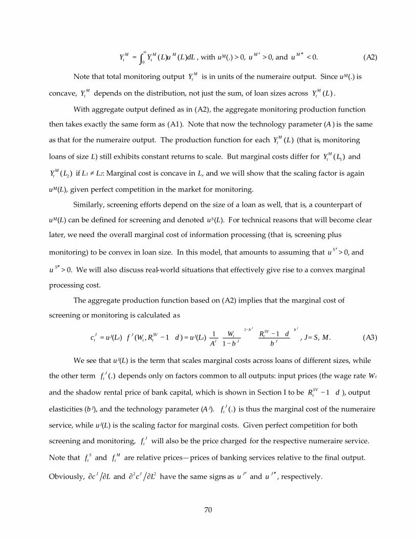
MtY =

0( ) ( )M M

tY L L dLυ∞

∫ , with υM(.) > 0, Mυ ′ > 0, and Mυ ′′ < 0. (A2)

Note that total monitoring output MtY is in units of the numeraire output. Since υM(.) is

concave, MtY depends on the distribution, not just the sum, of loan sizes across ( )M

tY L .

With aggregate output defined as in (A2), the aggregate monitoring production function

then takes exactly the same form as (A1). Note that now the technology parameter (A) is the same

as that for the numeraire output. The production function for each ( )MtY L (that is, monitoring

loans of size L) still exhibits constant returns to scale. But marginal costs differ for 1( )MtY L and

2( )MtY L if L1 ≠ L2: Marginal cost is concave in L, and we will show that the scaling factor is again

υM(L), given perfect competition in the market for monitoring.

Similarly, screening efforts depend on the size of a loan as well, that is, a counterpart of

υM(L) can be defined for screening and denoted υS(L). For technical reasons that will become clear

later, we need the overall marginal cost of information processing (that is, screening plus

monitoring) to be convex in loan size. In this model, that amounts to assuming that Sυ ′ > 0, and

Sυ ′′ > 0. We will also discuss real-world situations that effectively give rise to a convex marginal

processing cost.

The aggregate production function based on (A2) implies that the marginal cost of

screening or monitoring is calculated as

Jtc = υJ(Lt)⋅ ( , 1 )J SV

t tf W R δ− + = υJ(Lt)⋅1

111

JJSV

t tJ J J

W RA

ββδ

β β

− − + −

, J = S, M. (A3)

We see that υJ(L) is the term that scales marginal costs across loans of different sizes, while

the other term (.)Jtf depends only on factors common to all outputs: input prices (the wage rate Wt

and the shadow rental price of bank capital, which is shown in Section I to be 1SVtR δ− + ), output

elasticities (β J), and the technology parameter (AJ). (.)Jtf is thus the marginal cost of the numeraire

service, while υJ(L) is the scaling factor for marginal costs. Given perfect competition for both

screening and monitoring, Jtf will also be the price charged for the respective numeraire service.

Note that Stf and M

tf are relative prices—prices of banking services relative to the final output.

Obviously, Jc L∂ ∂ and 2 2Jc L∂ ∂ have the same signs as Jυ ′ and Jυ ′′ , respectively.

70

1.C Terms of the Loan Contract for Entrepreneurs’ Projects

We now describe terms of the loan contract, which will enter a bank’s optimization

problem in the subsection. For a penniless entrepreneur i born in period t (called generation-t) to

purchase capital 1itK + for his project, he must borrow 1

itK + plus the screening fee ( )1

S S it tf Kυ + . The

relative price of capital is 1, since there is one homogeneous good and no capital adjustment cost.

The subscript of 1itK + denotes the period in which the capital is used in production. S

tf and

( )1S i

tKυ + are as defined above: the unit fee and the amount of screening needed for a project of size

Ki. The entrepreneur then pays back ( )1 1i S S it t tK f Kυ+ ++ plus interest in period t+1. In effect, with no

internal funds, firms can compensate banks for the screening only by paying the fee (future value)

eventually at the end of period two from their projects’ payoffs.

The return on each project is subject to both project-specific and aggregate risk. Project i

arriving in period t pays 1i K

tRθ + for every unit of investment, where θ i is i’s idiosyncratic return,

and 1KtR + is the average ex post gross return across all potential projects, realized in period t +1. θi is

the project-specific risk parameter (that is, type) uncovered by bank screening process. θ i will be

shown to depend on i’s random draw from the distribution of project productivities, zi. So, θ i is

i.i.d. across time and projects and assumed to have a differentiable c.d.f. G(θ) over a non-negative

and bounded support, with E(θ) = 1. 1KtR + represents the aggregate risk and thus depends on the

realization of the aggregate productivity shock in period t +1, that is, At+1.62 What is relevant for

decision making in period t is the conditional distribution of 1KtR + , which depends on At’s serial

correlation. Denote the conditional c.d.f. simply as F( 1KtR + ), which is assumed to be differentiable

over a non-negative support. θ i is uncorrelated with 1KtR + , since zi and At+1 are uncorrelated.

62 Since RK depends on an aggregate risk, technically we need project-specific idiosyncratic noise for monitoring to be necessary in addition to screening. We can introduce an idiosyncratic shock ωi so that a project’s realized return becomes 1

i i KtRω θ + . ωi summarizes all the random disturbances that are uncorrelated

across projects and time. But for the purpose of determining the interest rate to charge on a loan, ωi is redundant because it has a symmetric effect to 1

KtR + . So the presence of ωi changes none of the qualitative

results regarding the terms of the loan contract (see the relevant discussion below for more details) and the measurement of bank output, but only increases the complexity of the model. Thus, we omit idiosyncratic risk in the model, and simply assume that liquidating bankrupt projects requires real resources.

71

The default probability is endogenous, depending on the interest rate charged on a loan.

There is a one-to-one mapping between the gross interest rate a solvent borrower i is supposed to

pay (call it 1itZ + ) and a threshold value of the aggregate risk 1

KtR + , call it 1

itR + , such that

( )1 1 1[ ]i i S S it t t tZ K f Kυ+ + ++ = 1 1

i i it tR Kθ + + .63

So 1( )itF R + is the default probability, that is, the borrower is solvent when 1

KtR + ≥ 1

itR + , and

defaults otherwise. 64 It is intuitive for borrowers to express the contractual interest rate using 1itR + ,

since the payoff from the project is his sole source of income for repayment. The project’s expected

return to lenders, gross of any informational cost, is 1 1( )i i it tR Kθ+ +F , where the expected rate of

return is ? ( 1itR + )≡ 1

1 1 1 10[1 ( )] ( )

itRi i K K

t t t tF R R R dF R+

+ + + +− + ∫ .

1.D Financial Intermediaries’ Optimization Problem

In this subsection, we solve for banks’ optimal production plan and pricing of loans. We

first consider banks that are fully funded by equity. The representative bank’s objective is to

maximize the present value of its cash flows, by choosing 1itR + (conditional on 1

itK + ), S

tN , MtN , and

BtI :

0BV =E0{ ( ) ˆ1

1 1 1 1 1 1 2ˆ1 0 01

{ [ ( )] ( ) ( ) ( )t H i K M M i i i i

t t t t t t tt

R K R f K dG K R dG K dGθ

ττ θθ υ θ θ θ θ

∞ − ∞ ∞

+ + + + + + +==

− + −∑ ∏ ∫ ∫ ∫{ { {

ˆ

1 2 1 1 1 1 10 0( ) ( ) ( ) ( ) }S S i M M i B B

t t t t t t tf K dG f K dG W N Iθ

υ θ υ θ∞

+ + + + + + ++ + − −∫ ∫{ { }, (A4)

subject to the constraints:

1 1ˆ( )i K

t tR Rθ+ += , (A5)

10( ) ( )S i

tK dGυ θ∞

+∫ = 1( ) ( )S SS S S

t t tA K Nβ β− , (A6)

ˆ

10( ) ( )M i

tK dGθυ θ+∫ = 1

1 1 1( ) ( )M MM M M

t t tA K Nβ β−+ + + , (A7)

63 Note the 1

itR + here is defined differently than the 1

itR + in Section I, which actually corresponds to 1

itZ + here.

64 It is easy to show that, with an idiosyncratic risk ωi, there remains a one-to-one mapping between a loan’s interest rate and its default probability as well as its expected gross return, even though the cutoff level can be defined only for the product of ωi and RK, but not for either separately.

72

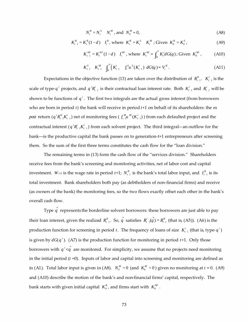
B S Mt t tN N N= + , and 0

MN = 0, (A8)

1 (1 )B B Bt t tK K Iδ+ = − + , where B S M

t t tK K K= + ; Given 0 0B SK K= , (A9)

1 (1 )NF NF NFt t tK K Iδ+ = − + , where NF

tK = 0

( )itK dG θ

∞

∫ ; Given 0NFK , (A10)

( )1 1 1 10( ) ( )S M i S S i

t t t t tK K K f K dGυ θ∞

+ + + ++ + +∫ = BtV . (A11)

Expectations in the objective function (13) are taken over the distribution of 1KtR + . 1

itK + is the

scale of type- iθ projects, and 1i i

tRθ + is their contractual loan interest rate. Both 1itK + and 1

itR + will be

shown to be functions of iθ . The first two integrals are the actual gross interest (from borrowers

who are born in period t) the bank will receive in period t+1 on behalf of its shareholders: the ex

post return ( 1 1i K i

t tR Kθ + + ) net of monitoring fees ( 1 1( )M M it tf Kυ+ + ) from each defaulted project and the

contractual interest ( 1 1i i i

t tR Kθ + + ) from each solvent project. The third integral—an outflow for the

bank––is the productive capital the bank passes on to generation-t+1 entrepreneurs after screening

them. So the sum of the first three terms constitutes the cash flow for the “loan division.”

The remaining terms in (13) form the cash flow of the “services division.” Shareholders

receive fees from the bank’s screening and monitoring activities, net of labor cost and capital

investment. Wt+1 is the wage rate in period t+1; 1BtN + is the bank’s total labor input, and 1

BtI + is its

total investment. Bank shareholders both pay (as debtholders of non-financial firms) and receive

(as owners of the bank) the monitoring fees, so the two flows exactly offset each other in the bank’s

overall cash flow.

Type θ̂ represents the borderline solvent borrowers: these borrowers are just able to pay

their loan interest, given the realized 1KtR + . So, θ̂ satisfies 1 1

ˆ( )i Kt tR Rθ+ += (that is, (A5)). (A6) is the

production function for screening in period t. The frequency of loans of size 1itK + (that is, type- iθ )

is given by dG( iθ ). (A7) is the production function for monitoring in period t+1. Only those

borrowers with iθ <θ̂ are monitored. For simplicity, we assume that no projects need monitoring

in the initial period (t =0). Inputs of labor and capital into screening and monitoring are defined as

in (A1). Total labor input is given in (A8). 0 0MN = (and 0 0MK = ) given no monitoring at t = 0. (A9)

and (A10) describe the motion of the bank’s and non-financial firms’ capital, respectively. The

bank starts with given initial capital 0BK , and firms start with 0

NFK .

73

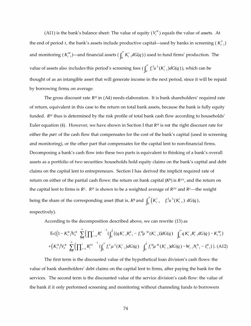
(A11) is the bank’s balance sheet: The value of equity ( BtV ) equals the value of assets. At

the end of period t, the bank’s assets include productive capital––used by banks in screening ( 1StK + )

and monitoring ( 1MtK + )––and financial assets ( 10

( )itK dG θ

∞

+∫ ) used to fund firms’ production. The

value of assets also includes this period’s screening fees ( 10( ) ( )S S i

t tf K dGυ θ∞

+∫ { ), which can be

thought of as an intangible asset that will generate income in the next period, since it will be repaid

by borrowing firms, on average.

The gross discount rate RH in (A4) needs elaboration. It is bank shareholders’ required rate

of return, equivalent in this case to the return on total bank assets, because the bank is fully equity

funded. RH thus is determined by the risk profile of total bank cash flow according to households’

Euler equation (4). However, we have shown in Section I that RH is not the right discount rate for

either the part of the cash flow that compensates for the cost of the bank’s capital (used in screening

and monitoring), or the other part that compensates for the capital lent to non-financial firms.

Decomposing a bank’s cash flow into these two parts is equivalent to thinking of a bank’s overall

assets as a portfolio of two securities: households hold equity claims on the bank’s capital and debt

claims on the capital lent to entrepreneurs. Section I has derived the implicit required rate of

return on either of the partial cash flows: the return on bank capital (KB) is RSV, and the return on

the capital lent to firms is RL. RH is shown to be a weighted average of RSV and RL––the weight

being the share of the corresponding asset (that is, KB and ( )1 10( ) ( )i S S i

t t tK f K dGυ θ∞

+ ++∫ ,

respectively).

According to the decomposition described above, we can rewrite (13) as

E0{ ( ) ( ) ˆ1

1 0 1 1 1 1 1 1 2ˆ1 01

1 { [( ( )] ( ) ( ) }tB B L i K M M i i i NF

t t t t t t tt

K V R K R f K dG K R dG Kθ

ττ θθ υ θ θ θ

∞ − ∞

+ + + + + + +==

− − + −∑ ∏ ∫ ∫{ {

+ ( ) ( ) ˆ1

1 0 1 2 1 1 1 1 11 0 01

{ ( ) ( ) ( ) ( ) }tB B SV S S i M M i B B

t t t t t t tt

K V R f K dG f K dG W N Iθ

ττυ θ υ θ

∞ − ∞

+ + + + + + +==

+ − −∑ ∏ ∫ ∫{ { }. (A12)

The first term is the discounted value of the hypothetical loan division’s cash flows: the

value of bank shareholders’ debt claims on the capital lent to firms, after paying the bank for the

services. The second term is the discounted value of the service division’s cash flow: the value of

the bank if it only performed screening and monitoring without channeling funds to borrowers

74

and households. 65 Then,

1S

tY + = 20( ) ( )S i

tK dGυ θ∞

+∫ { and 1M

tY + =ˆ

10( ) ( )M i

tK dGθυ θ+∫ {

are the implicit outputs of screening and monitoring services, respectively. 1S

tf + and 1M

tf + are the

respective shadow prices (that is, fee per numeraire loan), equal to the corresponding marginal

cost given perfect competition. RSV is determined by the risk of the service division, while RL is

determined by the risk of the loan division. Since services have the senior claim on total bank

income, RSV < RH < RL. In fact, RSV is lower than the risk free rate because 1M

tY + is negatively

correlated with 1KtR + and in turn the pricing kernel mt+1.

The implicit assumption behind the partition of total bank cash flow in (A12) is that bank

services are paid for first, before shareholders receive the residual as interest on their lending to

firms. We have explained in Section I that such a partition exactly maps into a rating agency plus a

bond issue. More importantly, this partition also maps into an activity common in today’s bank

operation––securitization. (A12) is essentially the same arrangement of cash flows as in a

securitization: Banks receive origination fees up front for screening borrowers and servicing fees

for payment transactions over the lifetime of loans in the loan pool. Investors in the loan pool then

receive the residual gross interest payments. Securitization provides a useful conceptual

benchmark for indirectly measuring the implicitly priced output of services in traditional banking.

Furthermore, it provides estimates of the fees of bank informational services which can be used

practically to impute the value of implicit bank output. See Section III for further discussion.

The realization of the aggregate technology shock At+1 determines the credit-worthiness of

generation-(t+1) firms and the defaults of generation-t firms. This in turn determines banks’

screening ( 1S

tY + ) and monitoring ( 1M

tY + ) outputs and the respective derived demand for labor, written

as follows:

1JtN + =

1 ( 1 )

1

1 1( )

J

J

Jt

J Jt t

Y

A K

β

β

−

+

+ +

, J = S and M.

The pre-chosen bank capital 1BtK + is allocated optimally between screening and monitoring:

65 Banks would become identical to rating agencies in this case, and firms would issue bonds directly.

75

1S

tMP+ = 1 1

1

S S St t

St

f YKβ+ +

+

= 1M

tMP+ = 1 1

1

M M Mt t

Mt

f YKβ+ +

+

, and 1 1 1B S Mt t tK K K+ + += + .

1.E The Determination of the Contractual Interest Rate

The loan division’s problem (the first component in (A12)) provides the decision rule for

setting the contractual interest rate on a loan. It contains all the relevant cash flows for the

debtholders, as it has internalized all the (expected) processing costs associated with a debt

contract. It expresses the condition that the interest rate the bank charges must generate an

expected return (net of the monitoring cost) that is no less than the ex ante rate of return required

by households on their investment (the capital rented by firms plus the screening fee), depending

on the systematic risk of the realized net cash flow. This condition must hold for every loan, to

avoid arbitrage. So, the choice of contractual interest rate (corresponding to the cutoff value 1itR +

for the aggregate risk) on a loan to a generation-t entrepreneur (i) must satisfy:

1

1 1 1 1 1 1 t 1 1 1 1 1 10[1 ( )] ( ) E [ ] ( ) ( ) [ ( )]

itRi i i i i K i K M M i i Li i S S i

t t t t t t t t t t t t tF R R K R K dF R f K F R R K f Kθ θ υ υ+

+ + + + + + + + + + + +− + − ≥ +∫ . (A13)

Note that the relevant discount rate for the risky debt return is RLi, but not RHi, that is, it is

the expected return on the partial cash flow corresponding to shareholders’ debt claim on firms,

but not a bank’s total cash flow. Note also that 1M

tf + is not known when 1itR + is chosen in period t,

so Et[ 1M

tf + ] is used in setting 1itR + . Since households are competitive in supplying capital for firms to

rent, (A13) holds with equality in equilibrium. Let 1Mi

tf + ≡ t 1 1E [ ] ( )M M it tf Kυ+ + and Si

tf ≡ 1( )S S it tf Kυ + ; then

1itR + satisfies:

1

1 1 1 1 1 1 1 1 1 10{[1 ( )] ( )} ( )

itRi i i i K K Mi i Li Si Li i

t t t t t t t t t t tK F R R R dF R f F R R f R Kθ+

+ + + + + + + + + +− + − − =∫ . (A14)

This is the key first-order condition from the bank’s maximization problem set up in (A4) to

(A11). The LHS of (A14) is the expected net return a lender will receive in period t+1 for funding

project i (denoted , 1ei tΠ + ). Evidently, information processing costs (that is, Si

tf and 1Mi

tf + ) depress

investment, since they raise the threshold of required intrinsic returns, for any given 1LitR + , and thus

shrink the set of profitable projects.

Note that, if measured in period t+1, bank screening reduces , 1ei tΠ + by 1

Li Sit tR f+ , which

76

exceeds Sitf by the time value, because Si

tf must be borrowed by the firm up front (that is, in

period t) and paid back at the end of the project (t+1). So the payment is in future va lue terms.

This mismatch of timing creates a problem for the measurement of true bank output, discussed in

detail in Section III.

An increase in 1itR + has two opposite effects on a lender’s return: It raises the marginal

return by 1 1[1 ( )]i i it tF R Kθ+ +− through a higher non-default payoff, and it also raises the cost by

1 1( )Mi it tf f R+ + because of a higher default probability. For a given project, these two effects exactly

offset at a cutoff level 1itR + , with 1( )i

th R + = 1 1i i Mi

t tK fθ + + , where ( ) ( ) [1 ( )]K K Kh R f R F R≡ − is the

hazard rate. If we restrict F( KR ) to satisfy

( )Kh R′ > 0, (A15)

then there is a unique interior solution of 1itR + , which maximizes lenders’ expected return.

Condition (A15) is weak and is satisfied by a number of common distributions such as the normal.

We limit our analysis to cases where 1itR + ≤ 1

itR + , in which range the expected return is increasing

and concave in the contractual interest rate. We also assume that the parameter values are such

that all the projects that are funded in an equilibrium are above the relevant minimum scales. 66

Neither restriction is central for our conclusions.

As intuition would suggest, condition (A14) implies that the higher banks’ costs of

processing information (that is, fMi and fSi), the higher the cutoff level 1itR + :

1

1

itMi

t

Rf

+

+

∂∂

= 1

1 1 1 1

( )[1 ( )] ( )

it

i i i Mi it t t t

F RF R K f f Rθ

+

+ + + +− −> 0, and 1

1

itSi

t

Rf

+

+

∂∂

= 1

1 1 1 1[1 ( )] ( )

Lit

i i i Mi it t t t

RF R K f f Rθ

+

+ + + +− −> 0, (A16)

since the identical denominator for both is positive, given the assumption 1itR + < 1

itR + . Also

intuitively, (A14) implies that the better a project’s type, the lower the cutoff level 1itR + , that is,

1 1i it tR θ+ +∂ ∂ < 0. By comparison,

1

1

itit

RK

+

+

∂∂

= 1 1 1 1

1 1 1 1

(1 ( ) ) ( ) ( ) ( )[1 ( )] ( )

Li Si Mi i i it t t t t

i i i Mi it t t t

R f f F R RF R K f f R

θθ

+ + + +

+ + + +

′ ′+ + −− −

F , (A17)

where 1( )Mitf +

′ ≡ 1 1Mi i

t tf K+ +∂ ∂ and ( )Sitf ′ ≡ 1

Si it tf K +∂ ∂ . So the sign of 1 1

i it tR K+ +∂ ∂ depends on the

numerator. Using (A14) to substitute for 1( )i itR θ+F , the numerator can be written as

66 See Wang (2004) for the definition of the relevant minimum scale and a detailed analysis of its properties.

77

1 1 1 1 1 1[( ) ] ( )[( ) ]Li Si Si i i Mi Mi it t t t t t t tR f f K F R f f K+ + + + + +

′ ′− + − . (A18)

Most likely, 1 1 1( )Mi i Mit t tf K f+ + +

′− > 0 and 1 ( )Si i Sit t tf K f+

′− > 0 for any 1itK + beyond a certain scale.

This is because 1 1 1 1[ ( ) ]Ji i Ji it t t tf K f K+ + + +

′∂ − ∂ > 0 (J = M, S), and it seems likely that monitoring

(screening) even a small loan involves a (fixed) cost that is greater than the extra cost of monitoring

(screening) a marginally bigger loan, that is, f Ji(ε) > (f Ji(ε))' for a small positive ε. If so, then (A18) is

always negative, and so

1 1i it tR K+ +∂ ∂ < 0, (A19)

meaning a lower contractual interest rate is needed to generate an expected rate of return of 1LitR +

for a larger loan-project.

Result (A19) is the opposite of that found in most other theoretical studies, which conclude

that, for a given borrower, ceteris paribus, the larger the loan size, the higher the interest rate. 67 The

derivations hitherto have made it clear that 1 1i it tR K+ +∂ ∂ > 0, because external funds cannot arise

from costs of standardized information processing, for which it is reasonable to assume that

( )Sitf ′′ < 0 and 1( )Mi

tf +′′ < 0. Other forms of costs are needed to yield 1 1

i it tR K+ +∂ ∂ > 0, which is a

necessary condition for a finite optimal Ki . (See Wang 2004, section 1.6.) Within the context of this

model, we can show that two realistic situations can generate a positive 1 1i it tR K+ +∂ ∂ : 1) if

entrepreneurs divert funds to unprofitable uses, and only bank monitoring can curb misuses, but

the marginal cost of reducing the fraction of funds misappropriated is increasing, or 2) if the effort

of entrepreneurs is an increasing but concave function of the intensity of bank monitoring. Since

the exact mechanism is unimportant for this model, we just assume that ( )Sitf ′′ >0 so that

1( )Si Si it t tf f K +

′ − > 0, and 1 1 1 1( ) ( )Si Si i Mi Mi it t t t t tf f K f f K+ + + +

′ ′− > − − . Then, (A18) is guaranteed to be

positive because Ri > 1 while F(Ri) < 1, and so 1 1i it tR K+ +∂ ∂ > 0.

1itR + also depends on the distribution of 1

KtR + , and the higher the mean project return, the

lower 1itR + . Denote the mean of 1

KtR + as 1

etR + , and define 1

Ktu + = 1

KtR + - 1

etR + and substitute for 1

KtR + .

67 Those studies obtain convex cost for external funds by introducing positive net worth for entrepreneurs, who then borrow against their net worth to invest. One exception is Froot and Stein (1998), who implicitly obtain the cost of funds as a decreasing function of project size, but an increasing function of the project’s leverage.

78

Then we can derive68

1

1

itet

RR

+

+

∂∂

= 1 1 1 1

1 1 1 1

( ) ( )[1 ( )] ( )

i i i Mi it t t t

i i i Mi it t t t

F R K f f RF R K f f R

θθ

+ + + +

+ + + +

+−− −

< 0, (A20)

since both the numerator and the denominator are positive.

1.F Optimal Choice of Capital by Non-Financial Firms

Given the debt contract described above, firm i chooses 1itK + to maximize the expected

utility of the owner-entrepreneur’s residual return, subject to the constraint (A14):

max Et( 1Uit + ) =

11 1 1 1max U[( ) ] ( )

it

K i i i Kt t t tR

R R K dF Rθ+

∞

+ + + +−∫ , (A21)

where U(.) is the utility function of entrepreneurs, with U(0) = 0, U′ > 0, and U′′ < 0. Clearly, 1itR +

and 1itK + are jointly determined by the bank and the firm’s optimization problems. Taking into

account that 1itR + is an implicit function of 1

itK + as defined by (A14), the first-order condition for

1itK + is:

11 1 1 1 1 1U (.)[( ) ( ) ] ( )

it

K i i i i i Kt t t t t tR

R R R K K dF Rθ+

∞

+ + + + + +′ − − ∂ ∂∫ = 0. (A22)

Equation (A22) makes it clear that, given any 1( )KtF R + , 1 1

i it tR K+ +∂ ∂ > 0 is a necessary

condition for a finite optimal 1itK + , since otherwise the left hand side (that is, t 1 1E (U )i i

t tK+ +∂ ∂ )

would always be positive, meaning all entrepreneurs would want to invest in projects as large as

possible.

Furthermore, since the production technology has constant returns to scale, the supply

curve for funds must be upward sloping (that is, 1 1i et tK R+ +∂ ∂ > 0) in order for an individual project

to have a finite scale. Fully differentiating (A22) with respect to 1itK + and 1

etR + yields

1

1

itet

KR

+

+

∂∂

= 2

1 1 1

1 1 1 1 1 12

1 1 12

1 1 1 1 1

(UR) ( U )1 1 1

( U ) (UR)1 1 1

( ) ( ) (U)

( ) (2 ) (U)

i i ii it t t

e i e e e it t t t t t

i i ii it t ti i i i it t t t t

R R Ri i i it t tR K R R R K

R R Ri i i it t tK K K K K

R K K

R K K

+ + +

+ + + + + +

+ + +

+ + + + +

′ ′∂ ∂ ∂∂ ∂+ + +∂ ∂ ∂ ∂ ∂ ∂

′ ′∂ ∂ ∂∂ ∂+ + +∂ ∂ ∂ ∂ ∂

′− + − +

′+ − + +,

where ( U )i′ ≡1

1 1U ( ) ( )it

KtR

r dF R+

∞

+′∫ , (UR)i′ ≡1

1 1 1U ( ) ( )it

K Kt tR

r R dF R+

∞

+ +′∫ , and 1 1 1 1( )K i i it t tr R R Kθ+ + +≡ − . Substituting

1Ktu + for 1

KtR + , and applying the above results for 1 1

i it tR K+ +∂ ∂ and 1 1

i et tR R+ +∂ ∂ , we can show

68 As defined, 1

Ktu + only differs from 1

KtR + in mean but does not change the variance of the distribution.

79

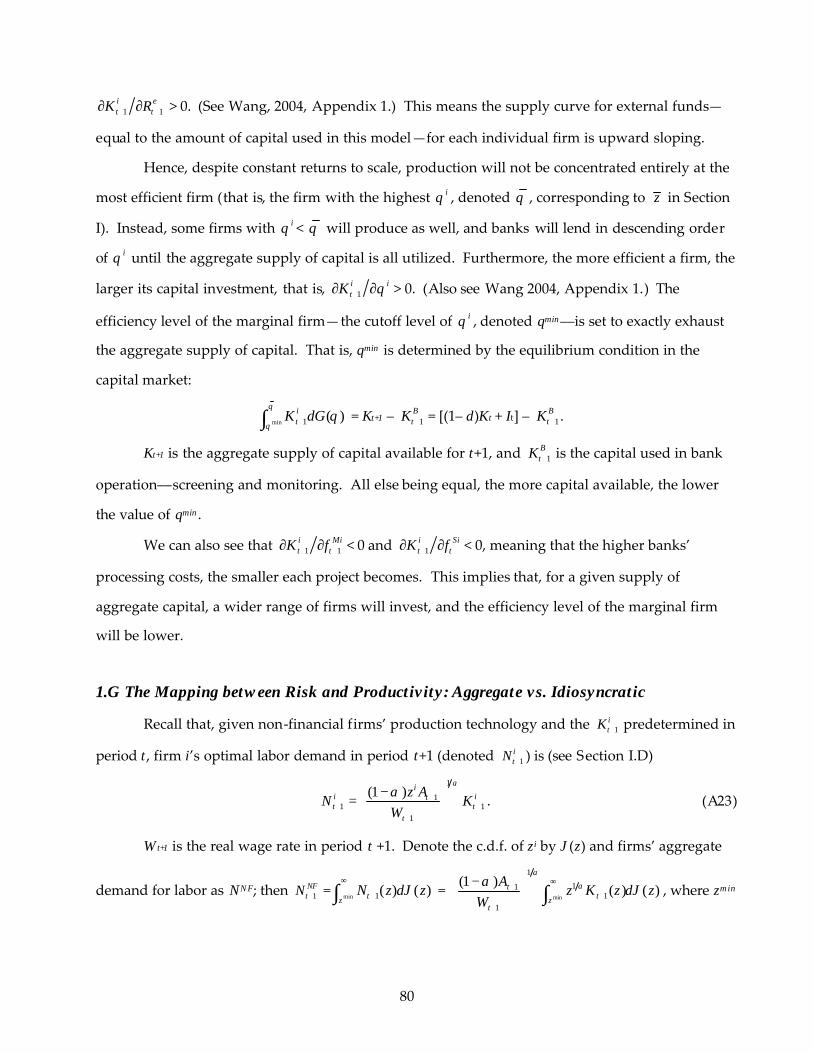
1 1i et tK R+ +∂ ∂ > 0. (See Wang, 2004, Appendix 1.) This means the supply curve for external funds—

equal to the amount of capital used in this model—for each individual firm is upward sloping.

Hence, despite constant returns to scale, production will not be concentrated entirely at the

most efficient firm (that is, the firm with the highest iθ , denoted θ , corresponding to z in Section

I). Instead, some firms with iθ < θ will produce as well, and banks will lend in descending order

of iθ until the aggregate supply of capital is all utilized. Furthermore, the more efficient a firm, the

larger its capital investment, that is, 1i itK θ+∂ ∂ > 0. (Also see Wang 2004, Appendix 1.) The

efficiency level of the marginal firm—the cutoff level of iθ , denoted θmin––is set to exactly exhaust

the aggregate supply of capital. That is, θmin is determined by the equilibrium condition in the

capital market:

min 1 ( )itK dG

θ

θθ+∫ = Kt+1 – 1

BtK + = [(1– δ)Kt + It] – 1

BtK + .

Kt+1 is the aggregate supply of capital available for t+1, and 1BtK + is the capital used in bank

operation––screening and monitoring. All else being equal, the more capital available, the lower

the value of θmin.

We can also see that 1 1i Mit tK f+ +∂ ∂ < 0 and 1

i Sit tK f+∂ ∂ < 0, meaning that the higher banks’

processing costs, the smaller each project becomes. This implies that, for a given supply of

aggregate capital, a wider range of firms will invest, and the efficiency level of the marginal firm

will be lower.

1.G The Mapping between Risk and Productivity: Aggregate vs. Idiosyncratic

Recall that, given non-financial firms’ production technology and the 1itK + predetermined in

period t, firm i’s optimal labor demand in period t+1 (denoted 1itN + ) is (see Section I.D)

1

11 1

1

(1 ) ii itt t

t

z AN K

W

αα +

+ ++

−=

. (A23)

Wt+1 is the real wage rate in period t +1. Denote the c.d.f. of zi by ϑ(z) and firms’ aggregate

demand for labor as NNF; then 1NFtN + = min 1( ) ( )tz

N z d zϑ∞

+∫ = min

1

111

1

(1 )( ) ( )t

tzt

Az K z d z

W

α

ααϑ

∞+

++

−

∫ , where zmin

80

is the idiosyncratic productivity level of the marginal firm that has positive investment. We will

show that this firm has θ =θmin.

Denote aggregate labor supply in period t+1 as Nt+1; then equilibrium in the labor market

requires that 1NFtN + + 1

StN + + 1

MtN + = Nt+1, that is,

min

1

111

1

(1 )( ) ( )t

tzt

Az K z d z

W

α

ααϑ

∞+

++

−

∫ + 1 ( 1 )

1

1 1( )

J

J

JM tJ S J J

t t

Y

A K

β

β

−

+=

+ +

∑ = Nt+1, (A24)

(A24) indicates that Wt+1 is a function of At+1, 1StA + , and 1

MtA + , and thus is stochastic as well.

Then, firm i’s ex post return on capital, that is, 1i K

tRθ + in above section 1.C, can be expressed as

1 1i KtRθ δ+ − + = 1 1 1

1

i it t t

it

Y W NK

+ + +

+

− =1 11

11

1( )i

tt

z AW

αα αα

−

++

−

≡1

( )iz α ϒ , (A25)

where ϒ ≡

111

11

1( )t

t

AW

αα α

α−

++

−

. So, there is a one-to-one monotonic mapping between zi and iθ ,

which we express as ( )i izθ θ= , and so zmin corresponds to θmin. It is intuitive that firm-specific

technology shock (zi) is the sole source for the idiosyncratic risk ( iθ ), whereas aggregate shocks

At+1, 1StA + , and 1

MtA + drive 1

KtR + .

We can now write the aggregate production function of the non-financial sector as follows,

where Yt+1 is aggregate output:

min

11 1 1 1[ ( ( ))] [ ( ( ))] ( )t t t tz

Y zA K z N z d zα αθ θ ϑ∞ −

+ + + += ∫ . (A26)

Then, the ex post rental rate of capital for the non-financial sector as a whole equals

1 1KtR δ+ − + = 1 1 1

1

NFt t t

NFt

Y W NK

+ + +

+

− =min

min

1111

1

11 1

[ ( ( ))] ( )1

[ ( ( ))] ( )

tzt

t tz

z K z d zA

W K z d z

αα

αθ ϑα

αθ ϑ

∞−+

+ ∞+ +

−

∫∫

. (A27)

The non-financial sector’s total capital stock 1NFtK + = min 1[ ( ( ))] ( )tz

K z d zθ ϑ∞

+∫ . Combining (A25) and

(A27), we obtain

1

( ) (1 )(1 )

ii z α δ

θκ δ

ϒ + −=

ϒ + −, where κ ≡ min

11 1( )i NF

t tzz K d z Kα ϑ

∞

+ +∫ , and ϒ is as defined above.

81

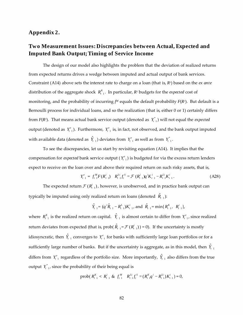
Appendix 2.

Two Measurement Issues: Discrepancies between Actual, Expected and Imputed Bank Output; Timing of Service Income

The design of our model also highlights the problem that the deviation of realized returns

from expected returns drives a wedge between imputed and actual output of bank services.

Constraint (A14) above sets the interest rate to charge on a loan (that is, Ri) based on the ex ante

distribution of the aggregate shock 1KtR + . In particular, Ri budgets for the expected cost of

monitoring, and the probability of incurring fM equals the default probability F(Ri). But default is a

Bernoulli process for individual loans, and so the realization (that is, either 0 or 1) certainly differs

from F(Ri). That means actual bank service output (denoted as *1tY + ) will not equal the expected

output (denoted as 1e

tY + ). Furthermore, 1e

tY + is, in fact, not observed, and the bank output imputed

with available data (denoted as 1t̂Y + ) deviates from 1e

tY + as well as from *1tY + .

To see the discrepancies, let us start by revisiting equation (A14). It implies that the

compensation for expected bank service output ( 1e

tY + ) is budgeted for via the excess return lenders

expect to receive on the loan over and above their required return on such risky assets, that is,

1e

tY + = 1 1 1 1 1 1 1( ) ( )M i Li S i i i Li it t t t t t t tf F R R f R K R Kθ+ + + + + + ++ = −F . (A28)

The expected return 1( )itR +F , however, is unobserved, and in practice bank output can

typically be imputed using only realized return on loans (denoted 1t̂R + ):

1t̂Y + = 1 1 1ˆ( )i L i

t t tR R Kθ + + +− , and 1t̂R + = min{ 1KtR + , 1

itR + },

where 1KtR + is the realized return on capital. 1t̂Y + is almost certain to differ from 1

etY + , since realized

return deviates from expected (that is, prob( 1t̂R + = 1( )itR +F ) = 0). If the uncertainty is mostly

idiosyncratic, then 1t̂Y + converges to 1e

tY + for banks with sufficiently large loan portfolios or for a

sufficiently large number of banks. But if the uncertainty is aggregate, as in this model, then 1t̂Y +

differs from 1e

tY + regardless of the portfolio size. More importantly, 1t̂Y + also differs from the true

output *1tY + , since the probability of their being equal is

prob( 1KtR + < 1

itR + & 1 1 1 1 1( )M Li S K i Li i

t t t t t tf R f R R Kθ+ + + + ++ = − ) = 0,

82

as monitoring will be performed only when default occurs.

In fact, 1t̂Y + and *1tY + are likely to be negatively correlated in reality, as in this model. In the

model, lenders’ ex post return is high while no monitoring is performed, and vice versa.

Specifically, when a loan is repaid, lenders receive a return exceeding expected costs of funds plus

processing, and so 1t̂Y + is relatively high ( 1t̂Y + > 1e

tY + ). At the same time, actual bank output is

relatively low ( *1tY + < 1

etY + ), since only screening is performed and no monitoring is necessary.

Conversely, when a borrower defaults, the return lenders receive is most likely less than expected

costs of funds plus processing, and so 1t̂Y + is relatively low.69 But *1tY + (> 1

etY + ) is relatively high since

monitoring must be conducted, given the default.70 Overall, the relationship among 1t̂Y + , *1tY + , and

1e

tY + can be summarized as follows:

Table A.1 Relationship between True Bank Output, and Imputed and Expected Bank Output

a) when 1KtR + ≥ 1

itR + ,

1t̂Y + > 1e

tY + > *1tY + .

b) when 1KtR + < 1

itR + , if b.1) 1

itR + > 1

ˆ itR + , then for i) 1

KtR + ∈ [ 1

ˆ KtR + , 1

itR + ),

1t̂Y + > *1tY + > 1

etY + .

ii) 1KtR + ∈ [ 1

KtR + , 1

ˆ KtR + ), *

1tY + > 1t̂Y + > 1e

tY + .

iii) 1KtR + < 1

KtR + , *

1tY + > 1e

tY + > 1t̂Y + .

if b. 2) 1itR + < 1

ˆ itR + , then for i) 1

KtR + ∈ [ 1

KtR + , 1

itR + ), *

1tY + > 1t̂Y + > 1e

tY + .

ii) 1KtR + < 1

KtR + , *

1tY + > 1e

tY + > 1t̂Y + .

69 It is possible that 1t̂Y + > 1

etY + even when 1

KtR + < 1

itR + , since 1

itR + > 1( )i

tR +F . Denote 1KtR + = 1( )i

tR +F , then for

1KtR + ∈ ( 1

KtR + , 1

itR + ], 1t̂Y + > 1

etY + .

70 If 1t̂Y + > 1e

tY + when a borrower defaults, then the relationship between 1t̂Y + and *1tY + depends. Define 1

ˆ KtR + as

the value of 1KtR + that satisfies 1 1 1 1 1 1

ˆ K i i Li i Mi Li Sit t t t t t tR K R K f R fθ+ + + + + += + + , that is, 1

ˆ KtR + covers both screening and

monitoring costs. In order to have 1ˆ K

tR + < 1itR + , at least 1

itR + should be sufficient to cover both fS and fM. Denote

such an 1itR + as 1

ˆ itR + , then 1

ˆ itR + satisfies 1

ˆ

1 1 1 10ˆ( ) ( )

itRi i i K K

t t t tK R R dF Rθ +

+ + + +−∫ = 1 1ˆ[1 ( )]i Mi

t tF R f+ +− . The relationship

between 1ˆ K

tR + and 1itR + can be derived by rewriting (A14) as 1 1 1 1 1

ˆ[ ( )] [1 ( )]K i i i i Mit t t t tR R K F R fθ+ + + + +− = −F . So

1 1 1 1 1 1ˆ [1 ( )] ( )K i i i i Mi i

t t t t t tR R F R K f f Rθ+ + + + + +∂ ∂ = − − > 0, and 2 21 1

ˆ K it tR R+ +∂ ∂ < 0. (See discussions of , 1

ei tΠ + earlier.) This

implies 1ˆ K

tR + > 1itR + when 1

itR + < 1

ˆ itR + , and vice versa , because 1

ˆ KtR + = 1

itR + at 1

ˆ itR + . Then, when 1

itR + > 1

ˆ itR + , for

realized returns 1KtR + ∈ [ 1

ˆ KtR + , 1

itR + ], even though the borrower defaults, 1t̂Y + is still greater than *

1tY + , that is, lenders realize a positive net return.

83

To diminish 1t̂Y + ’s deviation from *1tY + , some suggest using the average return on loans over

time instead of 1KtR + . That amounts to using 1

etY + instead of 1t̂Y + to approximate *

1tY + , since the

average loan return over time should converge to 1( )itR +F , assuming stationary 1

KtR + . But is the

implicit assumption | 1e

tY + - *1tY + | < | 1t̂Y + - *

1tY + | true? The summary of relationships among 1t̂Y + , *1tY + ,

and 1e

tY + shows that the assumption is true in only three of the six cases. Mapped into the real

world, Case a) seems to correspond best to the boom phase of business cycles, whereas Case b.1)

corresponds to recessions, since 1itR + depends negatively on average 1

KtR + , which tends to be low

during recessions. So, only when economic conditions are either particularly good (Case a) or bad

(Case b.1.iii) is 1e

tY + a better proxy for *1tY + than 1t̂Y + . That is, using the time-series average return on

loans does not necessarily generate a uniformly more accurate output value.

Another issue that may lead to errors in the measured bank output is the timing of income

receipts. This model describes an apparent misalignment between the production of bank services

and the receipt of compensation. Screening is conducted in the first period, but expenses are not

ultimately paid for until the second period. In order to recoup the unconditional screening cost

( Sitf ) incurred in the first period, banks in expectation charge 1

Li Sit tR f+ in the second period, which

includes the time value of Sitf that is proportional to the expected holding-period rate of return on

risky assets. If we measure bank output of screening services in the second period based on

1Li Sit tR f+ , we will not only face a mismatch between output and inputs but also overstate bank

output, unless the price index of screening services exactly offsets the bias. This measurement

error in output levels can be ignored if growth rates (calculated as log differences) are the variables

of interest, but in reality output growth rates may be subject to errors as well, to the extent that 1LitR +

is time-varying and the variation is not fully offset by the deflator for screening services.

Even if the timing issue may be alleviated in lending nowadays as banks increasingly

charge explicit origination fees upfront, it may potentially arise in other less-traditional banking

activities. Banking organizations (for example, bank holding companies) have been expanding

their scope and now engage in increasingly diverse financial activities. Similar timing problems

arise whenever information-processing services are compensated for implicitly together with risk-

based charges. For instance, subsidiaries of bank holding companies underwrite numerous

84

derivatives contracts (of varied terms and formats but mostly tied to changes in interest rates),71

and they typically charge a single fee for both the service and the risk-based value of a contract.

Similarly, investment banks typically charge a single underwriting fee to cover both their

operating expenses and their risk exposure to uncertain demand for the security underwritten and

to the security’s uncertain returns on the market.

71 By the end of 2002, the absolute fair market value of derivatives held by the commercial banking industry totaled over $3 billion, compared with $231 billion of net interest income. See Carlson and Perli (2003).

85