a fluid-structure interaction simulation capability using the

1 2010 SIMULIA Customer Conference

A Fluid-Structure Interaction Simulation Capability Using the Co-Simulation Engine

Eric L. Blades1, Edward A. Luke2, Albert G. Kurkchubashe3, Eric M. Collins2, and R. Scott Miskovish1

1ATA Engineering, Inc., San Diego, CA 92130 2Mississippi State University, Starkville, MS 39762 3Dassault Systèmes, SIMULIA, Fremont, CA 94538

Abstract: A multiphysics simulation capability suitable for fluid-structure interaction is presented that uses the Abaqus nonlinear structural dynamics solver and the Loci/CHEM computational fluid dynamics solver. The coupling is achieved using SIMULIA’s Co-Simulation Engine technology. The Co-Simulation Engine is a software component that allows the coupling of multiple simulation domains by coupling solvers in a synchronized manner. Keywords: aeroelasticity, co-simulation engine, computational fluid dynamics, coupled analysis, fluid-structure interaction, flutter.

1. Introduction

The design of hypersonic vehicles represents a very challenging problem and requires simultaneous integration from multiple disciplines in order to achieve an efficient design. The hypersonic heating environment creates severe technology challenges for materials and structures that not only carry the aerodynamic loads but also repeatedly sustain high thermal loads, requiring long life and durability while minimizing weight. The severe heating environment encountered during hypersonic flight dictates the shape of the vehicle. Boundary layer transition and turbulence at hypersonic speeds are especially significant because of the large differences in heating rates between laminar and turbulent flows. Shock-shock interaction, for example, the interaction of the bow shock with inlet shocks, and shock-boundary layer interaction can lead to local enhancement of heating at the impingement point. Thus, the accurate definition and characterization of the hypersonic environment is of paramount importance. With the difficulty and expense of replicating the hypersonic environment using ground-based facilities, there is a great emphasis on developing suitable computational tools to define the environment. Accurate computational tools are needed for vehicle design using a physics-based multidisciplinary approach. The overarching purpose of this effort is to develop a multiphysics framework suitable for hypersonics analysis and the design of hypersonic vehicles. The focus of this paper is to describe the SIMULIA Co-Simulation Engine, with validation of the fluid-structure coupling. Note, however, that due to the high temperatures involved in hypersonic flow, the hypersonics multiphysics framework will require the inclusion of thermal effects and involve fluid-thermal-structural coupling. The multiphysics simulation is conducted using a loosely coupled but tightly


integrated domain decomposition approach. In a domain decomposition approach, the governing equations of motion for each domain (e.g., the fluid domain and the solid or structural domain) are solved using approaches or methods most appropriate for that domain. A computational fluid dynamics (CFD) code is integrated with a nonlinear computational structural dynamics (NLCSD) code in a fully coupled, fluid-structure interaction form. The CFD code to be coupled is Loci/CHEM and the NLCSD code is Abaqus/Explicit. The coupling of the CFD and NLCSD codes is done using SIMULIA’s Co-Simulation Engine (CSE) software. The Co-Simulation Engine is a software component that enables co-simulation and consists of a runtime environment that synchronizes the applications, coordinates communication, and provides spatial and temporal mapping at the domain interface.

2. SIMULIA Co-Simulation Engine

In an effort to inject more realism into simulation, SIMULIA has commenced on a multiphysics initiative to bring multiple physical representations into simulations in order to capture the real-world phenomena. As part of this initiative, SIMULIA is building the Co-Simulation Engine (CSE), a software component for enabling co-simulation between discrete and continuum systems. Examples of such coupled simulation include fluid-structure interaction and cyber-physical systems. The development is a multiyear effort in which the Co-Simulation Engine is delivered in stages with increasing complexity. SIMULIA is working closely with select partners and customers who are providing early feedback and design validation. ATA Engineering, Inc., and Mississippi State University are using this early form for coupling Loci/CHEM with Abaqus/Explicit for supersonic fluid-structure interactions. The CSE consists of several software components. The controller is a customizable state machine in charge of marshaling the clients, negotiating time, and ensuring that the physics fields are exchanged in a synchronized manner. Currently, the CSE supports explicit coupling schemes, both serial (Gauss-Seidel type) and concurrent (Jacobi type). Future versions will support coupling schemes for stronger coupled physics, including iterative schemes. The mapper provides both spatial and temporal mapping of the physics fields. Spatial mapping includes surface-based coupling in which the domains remain distinct and are coupled through a common surface, and volume-based mapping in which the physical domains overlap. Discrete data (e.g., signals between sensors and actuators) may also be exchanged between logical and physical systems. The spatial mapping between the domains is conservative. For example, Loci/CHEM may provide traction vectors on triangular cell centers that are then interpolated to nodal forces on a quadrilateral interface mesh on the Abaqus model. Furthermore, the CFD model may use a much finer discretization than the computational solid mechanics (CSM) model, which is more appropriate to its numerical treatment. The only restriction is that both the models need to be co-located in space. The communication layer is in charge of communicating both control and data messages between the controller and the clients. The CSE uses separate communication channels for control and bulk data. Bulk data are communicated directly between the clients (the “solvers”). Finally, the application programming interface (API) layer provides the interface to the client. The API is a C language interface providing a flexible, easy-to-use interface that allows C, C++, and FORTRAN clients to be integrated. From the clients’ perspective, the API is general and


transparent—that is, clients are unaware of the codes involved in the employed co-simulation and coupling algorithm.

2.1 Fluid-structure interaction coupling

In a domain-decomposition approach to a coupled fluid-structure interaction (FSI) problem, the CFD code will compute the pressure or traction vector at the fluid-structure interface (or wetted surface), and the NLCSD code will compute the resulting structural displacements due to those loads. The overall procedure for a typical FSI problem is illustrated in Figure 1 and is as follows when the CFD code leads:

1. Obtain the CFD solution at time level, n, and compute the nodal traction vector, ( )nfwT ,r

, acting on the fluid interface, f .

2. Map the nodal traction vector, ( )nfwT ,r

, from the nodes of the fluid interface to a nodal

force vector, ( )nswF ,r

, at the nodes of the solid interface, s, in a conservative manner.

3. Obtain the NLCSD solution to compute the displacements of the elastic body.

4. Map the displacements, ( )1, +nswxr , from the nodes of the solid interface to the nodes of the

fluid interface, ( )1, +nfwxr , in a conservative manner.

5. Move the interior CFD computational domain to reflect the structural deformation (i.e., volume grid adaptation).

6. Repeat for time level n+1.

Figure 1. Fluid-structure co-simulation data mapping procedure.

Since we are utilizing a domain-decomposition approach, each domain will be suitably discretized for the appropriate solver. As such, the interface between the two domains will almost certainly be discretized differently and will not match. The data transfer at the wetted surface interface is done using the mapping tools provided by the Co-Simulation Engine. Once the CFD wetted surface is moved to conform to the structural deformations, the flow solver adapts the volume grid to reflect these changes. The volume grid adaption is discussed in Section 4.2.


As previously mentioned, the hypersonic multiphysics simulation will involve fluid-thermal-structural coupling. In addition to the transferring and mapping the fluid (traction) and structural (displacement) quantities, thermal information such as heat flux and temperature will also be transferred at the interface.

2.2 Controlling the co-simulation

The Co-Simulation Engine provides various options for coupling the physical domains. To date, the most common explicit coupling schemes—the Gauss-Seidel and Jacobi methods—are being implemented. These schemes are appropriate for problems that exhibit weak to moderate coupling strength between the physics domains, as is expected for the application between Abaqus/Explicit and Loci/CHEM presented in this paper. When choosing a Gauss-Seidel algorithm, the solvers are run in tandem. Here the user has the option to select whether the CFD or the CSM code leads the simulation. When selecting the Jacobi algorithm, both solvers execute in parallel. The Jacobi algorithm has the advantage of utilizing the computing resources when both applications are run on different processors. However, in general, the Jacobi coupling scheme is less stable than the Gauss-Seidel algorithm. The Jacobi coupling scheme may be appropriate when coupling two solvers that use explicit time integrations, such as Abaqus/Explicit and Loci/CHEM. The rendezvousing schemes define the frequency of how often data are exchanged. The target time—when fields exchange between the clients—is negotiated with the input of both clients’ preferred increment sizes. The user has the option of selecting a constant coupling step size or using the minimum, maximum, or one of the client’s preferred coupling step sizes to determine the next target time. The client may subcycle, i.e., take increments/time steps smaller than the coupling step size, to reach the target time. One can also enforce a lockstep behavior in which the client’s increment/time step size needs to adhere to the coupling step size dictated by the CSE. When subcycling, the CSE provides suggested increment sizes such that the target time can be reached with a uniform size increment equal to or smaller than that preferred by the client.

3. Abaqus Unified Finite Element Analysis Suite

The Abaqus Unified finite element analysis (FEA) product suite offers powerful and complete solutions for both routine and sophisticated engineering problems covering a vast spectrum of industrial applications. Abaqus/Standard employs solution technology ideal for static and low-speed dynamic events where highly accurate stress solutions are critically important. Abaqus/Explicit is a finite element analysis product that is particularly well suited to simulating brief transient dynamic events. Both products provide nonlinear analysis that supports nonlinear materials, large displacements, finite rotations, and general contact. The solvers are parallel and run on shared memory and distributed memory clusters. Abaqus/Explicit and Abaqus/Standard are supported within the Abaqus/CAE modeling environment for all common pre- and postprocessing needs.

4. CHEM CFD Code

The Loci/CHEM code is a modern multiphysics simulation code that is capable of modeling chemically reacting multiphase high- and low-speed flows. CHEM is written in the Loci


framework (Luke, 2005) and is a Reynolds-averaged Navier-Stokes, finite-volume flow solver for generalized or arbitrary polyhedra, developed at Mississippi State University. CHEM (Luke, 2007a) uses density-based algorithms and employs high-resolution approximate Riemann solvers to solve finite-rate chemically reacting viscous turbulent flows. It supports adaptive mesh refinement (Luke, 2008), simulations of complex equations of state including cryogenic fluids (Luke, 2007b), multiphase simulations of dispersed particulates (Tong, 2005) using both Lagrangian and Eulerian approaches, conjugate heat transfer through solids (Liu, 2005), and non-gray radiative transfer associated with gas and particulate phases (Rani, 2008). Loci is a novel software framework that has been applied to the simulations of nonequilibrium flows. The Loci system uses a rule-based approach to automatically assemble the numerical simulation components into a working solver. This technique enhances the flexibility of simulation tools, reducing the complexity of CFD software induced by various boundary conditions, complex geometries, and varied physical models. Loci plays a central role in building flexible goal-adaptive algorithms that can quickly match numerical techniques with various physical modeling requirements. Loci, with its sophisticated automatic parallelizing framework, and Loci/CHEM have demonstrated scalability to problems in size exceeding one hundred million cells and have demonstrated production scalability to nearly one thousand processors. The Loci/CHEM CFD code is a library of Loci rules (fine-grained components) and provides: primitives for generalized grids, including metrics; operators, such as gradient; chemically reacting physics models, such as equations of state, inviscid flux functions, and transport functions (viscosity, conduction, and diffusion); a variety of time and space integration methods; linear system solvers; and more. Moreover, it is a library of reusable components that can be dynamically reconfigured to solve a variety of problems involving generalized grids by changing the given fact database, adding rules, or changing the query.

4.1 Integration of the CSE API

The coupling of domain-specific solvers to the SIMULA Co-Simulation Engine is accomplished through calls to CSE API. These calls provide mechanisms for synchronization and data transfer between two or more solvers running concurrently. A specific sequence of API calls must be made to establish the connection between the running solver instances and to manage the subsequent data transfer events. Since the CHEM CFD solver is implemented in the Loci framework, there is no explicit flow control available to manage this sequence. Rather, the sequence of execution is controlled by data dependencies. That is to say that if value C depends on A and B, (C A, B), then the rule that describes the computation of C will not be executed by Loci until the rules that compute A and B have completed. The proper ordering for the CSE API calls is established within CHEM by utilizing a series of rules that compute dummy variables. By providing these variables with appropriate data dependencies, the correct ordering of synchronization and data transfer events is assured. In the current implementation, the CHEM CFD solver leads the ABAQUS solid mechanics solver. First, CHEM signals the CSE that it is about to begin a fluid solution step. The fluid flow solution about the current geometry configuration is then obtained for a given time step. From this solution, the traction force vectors are computed from the momentum flux expressions on the fluid-solid boundary interface. These traction vectors are then transferred to Abaqus through the CSE, and CHEM signals that it has completed the fluid solution step. Abaqus solves the solid mechanics


equations of motion and returns to CHEM a set of displacements for the nodes on the fluid-structure interface. CHEM then performs a mesh adaptation step in which the nodes in the fluid domain are moved in response to the boundary displacement in such a way as to preserve desirable mesh spacings, such as for high-aspect-ratio boundary layer meshes that are typically used to resolve the fluid physics in the boundary layer. CHEM then signals that it is ready to begin the next solve step and the above process is repeated.

4.2 Volume grid deformation approach

To accomplish the goal of deforming the mesh, there are several methods available that fall roughly into two categories of approaches: ones that utilize the existing mesh connectivity, and ones that move each point based on an interpolation/extrapolation of deformations at boundary surfaces. The techniques that move the mesh based on mesh connectivity usually rely on physical analogs such as torsional springs (Farhat, 1998) (Degand, 2002) or elastic deformation (Stein, 2003), while the interpolation techniques involve simple use of distance weighted averages (Witteveen, 2009) or sophisticated radial basis function techniques (de Boer, 2007). Torsional springs and elastic deformation analogies are similar in structure, and both require solving a large sparse linear system. Elastic deformation approaches can have difficulties maintaining valid cells when using high aspect ratio cells unless care is taken to ensure that the solution to the linear system is adequately converged. Due to the high aspect ratio, this typically requires convergence criteria on the order of machine zero and is computationally expensive. High aspect ratio cells are typically used in high Reynolds number simulations in order to minimize the cell count. A simple interpolation-based approach is utilized to mesh deformation, which uses reciprocal distance weighed averages of rotation and displacements of surface nodes. Rotations of the surface about local nodes are computed using a nonlinear least squares method; the resulting deformation in the volume is computed using the equation

( ) ( ) ( )( )∑

∑=rw

rsrwrs

i

iir

rrr

(1)

where rr is the position vector, ( )rsir

is the displacement field about surface mesh point i , and

( )rwir

is the weight assigned to the mesh point given by

( )⎥⎥⎦

⎤

⎢⎢⎣

⎡⎟⎟⎠

⎞⎜⎜⎝

⎛−

+⎟⎟⎠

⎞⎜⎜⎝

⎛−

=b

i

defa

i

defii rr

Lrr

LArw

||||||||* rrrr

r α (2)

The sum given in equation (1) is evaluated approximately using a tree-code-based method that reduces the cost of the mesh deformation to ( )nnO log . We have been able to show that this method is able to produce large mesh deformations with good mesh quality while also maintaining mesh spacing and orthogonality in the highly anisotropic viscous mesh region.


5. Aeroelastic Validation Cases

A description of the two aeroelastic validation cases is described in the following sections. The first is a static aeroelastic case for which there are experimental data that can be used for validation; the second is a dynamic case for which computational data are available for validation.

5.1 Static aeroelastic validation case

The first fluid-structure interaction validation case is a static aeroelastic case using the ARW-2 wing-body configuration (Sandford, 1989) (Sandford, 1994) (Byrdsong, 1990). The ARW-2 was the second in a series of aeroelastic research wings developed at NASA Langley Research Center to experimentally study transonic steady and unsteady phenomenon in the Transonic Dynamics Tunnel. This research wing has an aspect ratio of 10.3, a leading edge sweep angle of 28.85°, and supercritical airfoil sections. The test configuration consisted of the ARW-2 high-mounted on a rigid half-body fuselage. Further details about the configuration can be found in (Sandford, 1989). The experimental study consisted of an enormous number of test conditions (Sandford, 1994) (Byrdsong, 1990). These test conditions studied variations in free-stream Mach number, angle of attack, dynamic pressure, and control surface deflections. Furthermore, tests were conducted in both a heavy gas and an air medium. The results presented herein correspond to a free-stream Mach number of 0.8, a dynamic pressure of 102.5 psf, with an air medium, and at a single angle of attack. The Reynolds number was Re = 2.1x106 based on a root chord of 38.9 inches. Control surface deflections were not considered.

5.1.1 Structural model

The ARW-2 wind tunnel test model represents a complex built-up structure that includes a composite fiberglass skin. The wing bending (EI) and torsional stiffness (GJ) properties are specified as equivalent beam properties along the elastic axis of the wing (Sandford, 1989). Therefore, a simple beam model along the elastic axis is used to represent the wing. It should be noted that it is well established that the deformation of high-aspect-ratio wings are consistent with classical beam theory and thus is a reasonable modeling assumption. The measured total wing weight is 156.25 lb; however, the mass distribution data are not provided (Sandford, 1989). Therefore, the weight of the wing will be accounted for by deflecting the wing due to a 1 g loading, i.e., the deflection of the wing due to its own weight. This deflected configuration is referred to as the wind-off position (WOP) and is the measured position of the wing when the tunnel is not in operation. This will be the starting configuration for the fluid-structure interaction cases. An ABAQUS finite element model (FEM) of the ARW-2 wing is shown in Figure 2 and illustrates the elastic axis beam model and the virtual computational structural dynamics (CSD) wetted surface. A total of 56 beam B31 elements was used to model the wing. Since the wing is modeled structurally using beam elements, a virtual CSD wetted surface is needed to facilitate the force and displacement transfer between the CSD and CFD models. The virtual wetted surface was constructed using ABAQUS surface elements (SFM3D4), which have no inherent mass or stiffness. The virtual surface was created by generating a structured surface grid, with the same spanwise point distribution as the wing elastic axis beam model. In order for the CSD virtual


surface to follow the deflection of the elastic axis beam model, the nodes on the virtual wetted surface are connected to the nodes on the elastic axis using kinematic coupling elements. At each spanwise location, all the points on the virtual CSD wetted surface are connected via kinematic coupling elements to the corresponding grid point on the elastic axis. Connecting the virtual surface to the beam in this manner enforces the assumption from beam theory that plane sections remain plane. After the CFD forces are mapped to the CSD wetted surface, the forces on the virtual surface are transferred to the elastic axis via modeling the kinematic coupling elements. For these fluid-structure interaction cases, the fuselage is assumed to be rigid and will be held fixed; thus, no structural representation is needed.

Figure 2. Finite element model and wetted surface for the ARW-2.

5.1.2 CFD model

A representative view of the CFD surface grid for the ARW-2 wing-body configuration is shown in Figure 3. The surface mesh for the wing wetted surface contains 61,646 nodes and 123,138 triangular boundary faces. SolidMesh (Gaither, 2000) was used to create the geometry and CFD surface mesh for the ARW-2 test configuration. The wind tunnel walls were not explicitly represented. Instead, a symmetry plane and a hemispherical far-field boundary (located a distance of ten semi-spans away from the body) were used to represent the boundaries of the domain. Both inviscid and viscous volume meshes were generated using the advancing-front/local-reconnection (AFLR) technique (Marcum, 2001), and the same surface mesh was used for each. The inviscid volume mesh consists of 1.3M nodes and 7.3M tetrahedra. The viscous volume mesh contains 4.0M nodes and 2.7M tetrahedra and nearly 7.0M prism elements in the boundary layer region. The normal spacing of the first grid point from the body was 4.0x10-4 inches and resulted in a y+ distribution of less than 1.0 over the wing and fuselage—thus indicating good viscous sublayer resolution.


The inviscid flux formulation used for the results presented here is based on an adaptive approximate Riemann solver (Quirk, 1992). The viscous simulations used Menter’s model (Menter, 1994), which utilizes the κ – ω model in the near wall region and gradually switches to the κ – ε model away from the wall. The turbulence model includes compressibility corrections for high-speed shear flows (Wilcox, 1998).

(a) (b)

Figure 3. ARW-2 CFD surface mesh (a) and detailed view (b).

5.1.3 ARW-2 results

Static aeroelastic analyses were conducted at the aforementioned test conditions for angles of attack varying from -2.0 to +4.0°. The results presented here are for the 0° case. For each angle of attack, steady state solutions were obtained for the rigid wing in the wind-off position, and the coupled aeroelastic solutions were restarted from these rigid wing solutions. The convergence criterion was defined to be less than a 0.01% change in the normal force (predominantly lift) over each of the last 100 iterations, and convergence was usually obtained in less than 1000 iterations. A comparison of experimentally measured and computed pressure coefficient data is shown in Figure 4 for two spanwise stations. The results from the viscous solution compare quite well with the measured data. As expected, the inviscid solution overestimates the pressure on the suction side and results in a higher lift force. The inviscid solution also tends to overpredict the strength of the shock on the upper surface. A comparison of the front and rear spar deflection is shown in Figure 5. The spar locations for the WOP are also included to help quantify the deflections; the measured tip deflection is approximately 2.9 inches. Very good agreement is obtained with the viscous solution with a difference of about 3.5% at the wing tip. Due to the estimation of the lift, the inviscid solution results in significantly higher displacements. At the tip, the inviscid deflection is 3.89 inches, resulting in a difference of 33%.


(a)

(b)

Figure 4. Comparison of measured and predicted pressure coefficient distribution at 55.9% (a) and 87.1% (b) span locations.


Figure 5. Comparison of measured and predicted spar deflections.

5.2 Dynamic aeroelastic validation case As opposed to the first test case, which was a steady state problem, the second test case is a two-dimensional elastic airfoil involving unsteady flow. The unsteady flow induces vibration of the airfoil and, depending upon the air speed, the response is either stable (damped), unstable (undamped), or neutrally stable. The NACA 64A010 airfoil has two structural degrees of freedom; it is allowed to pitch about a given elastic axis and plunge vertically and simulates the bending and torsion motion of a wing cross section. The model is shown in Figure 6a. The elastic axis is located a distance ba from the mid-chord position, and the center of gravity is located a distance bxα from the mid-chord position; note that if a is positive, then the elastic axis is located aft of the mid-chord, and if a is negative the elastic axis is located forward of the mid-chord. This is true for the center of gravity location as well.

Figure 6. Schematic of the Isogai elastic wing model and CFD mesh.


5.2.1 Elastic airfoil governing equations and finite element model

The governing equations for the two-dimensional elastically mounted airfoil can be written as

ea

h

MKIhS

LKShm

=++

−=++

ααα

α

α

α&&&&

&&&& (3)

where m is the airfoil mass per unit span, αS is the static mass moment (per unit span) about the

elastic axis, αI is the rotational mass moment of inertia (per unit span) about the elastic axis, hK

is the bending spring stiffness, αK is the torsional spring stiffness, L is the lift per unit span

(positive up), eaM is the moment per unit span about the elastic axis (positive nose up), and h and α are the plunging (positive down) and pitching (positive leading edge up) coordinates, respectively. The equations of motion can be nondimensionalized by using the uncoupled natural frequency of the torsional spring as the time scale, taωτ = , and the semi-chord b as the reference length. The resulting nondimensional mass and stiffness matrices are given by

M[ ]=1 xα

xα rα2

⎡

⎣ ⎢

⎤

⎦ ⎥ , K[ ]=

ωh

ωα

⎛

⎝ ⎜

⎞

⎠ ⎟

2

0

0 rα2

⎡

⎣

⎢ ⎢ ⎢

⎤

⎦

⎥ ⎥ ⎥ (4)

where mbSx α

α = is the dimensionless static unbalance and represents the coupling of pitch

and plunge degrees of freedom, rα = Iαmb2 is the dimensionless radius of gyration, hω is

the uncoupled natural bending frequency, αω is the uncoupled natural torsional frequency,

μ =m

πρb2 is the airfoil mass ratio, kc =ωcU∞

is the reduced frequency or Strouhal number, ρ is

the air density, c is the airfoil chord, and ∞U is the free-stream velocity.

The elastic model uses the following structural parameters corresponding to the Isogai wing model case A (Isogai, 1979): αx = 1.8, 2

αr = 3.48, a = -2.0, hω = 100 rad/sec, αω = 100 rad/sec, and μ = 60. These parameters are representative of an outboard section of a sweptback wing where the elastic axis is half of a chord length ahead of the leading edge of the airfoil. For this choice of parameters, the airfoil exhibits a dramatic reduction in the flutter speed in the transonic region, often referred to as the “transonic dip.” User-defined elements were employed to define the dimensional mass and stiffness matrices explicitly. Similar to the ARW-2 case, a virtual surface is needed to facilitate the force and displacement transfer between the CSD and CFD models. The virtual wetted surface was


constructed using ABAQUS rigid elements (R3D4), which have no inherent mass or stiffness. The virtual surface was defined to be a rigid body and connected to the pitch and plunge degrees of freedom.

5.2.2 Isogai CFD model

NACA 64A010 airfoil is used for the wing section. The inviscid volume mesh consists of 58,416 nodes and 76,884 prisms and was constructed by extruding the surface mesh shown in Figure 6b into a volume mesh that is two elements thick. The far-field boundary extends ten chord lengths from the airfoil. It should ne noted that the mesh for the CSD virtual wetted surface is the same as that used for the CFD surface mesh. No viscous simulations were conducted for the Isogai airfoil case.

5.2.3 Isogai airfoil results

The airfoil response was computed for different Mach numbers and different values of the flutter

speed index, which is defined as μωαb

UVF∞= . Similar to the ARW-2 cases, the aeroelastic

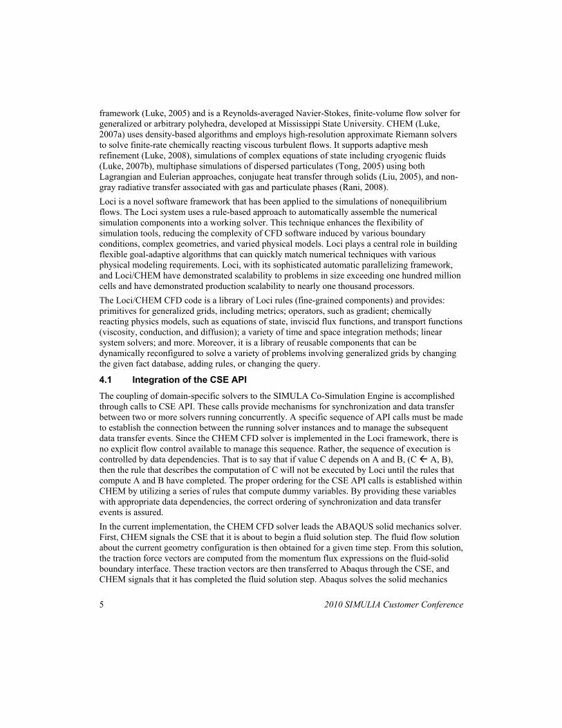
solutions were started from a steady state solution representing a specified altitude. Due to the symmetric nature of the airfoil, an initial perturbation was applied by specifying an angular velocity. The binary flutter mechanism represented by this system is a stability problem. At low values of the speed index, the system is stable and the response due to the initial perturbation damps out. As a speed index increases, the system becomes less and less stable until one or both of the degrees of freedom begins to increase in amplitude, and the response diverges and the system becomes unstable. In between these two conditions, there is a particular point where the system is neutrally stable, i.e., the flutter point. This process is repeated for each Mach number to define the flutter boundary. Once a stable and an unstable condition are identified, a simple bisection method is used to estimate the neutral point. Multiple cases are examined to compute each point on the boundary in order to determine a neutral or zero damping response. A comparison of the calculated flutter boundary with those of previous references is shown in Figure 7 (Blades, 2007), (Alonso, 1994), (Liu, 2001), (Chen, 2004), (Edwards, 1983). Overall, the present results compare very well and are able to predict the “transonic dip” phenomenon. The Mach number at the bottom of the transonic dip is 0.875 with a speed index of 0.45 and is consistent with results from the aforementioned cited literature.


Figure 7. Computed flutter boundary for the Isogai aeroelastic model.

6. Conclusions

A multiphysics simulation capability suitable for fluid-structure interaction problems has been presented that uses the Abaqus nonlinear structural dynamics code and the Loci/CHEM computational fluid dynamics code. The coupling is achieved using Simulia’s Co-Simulation Engine technology. The CSE is a software infrastructure that allows the coupling of multiple simulation codes and handles the code synchronization and information transfer between the different domains. Static and dynamic aeroelastic test cases were presented to validate the multiphysics capability; good agreement was obtained for each case.

7. Acknowledgements

This work was completed with SBIR funding from Wright-Patterson AFB, contract FA8650-09-M-3930, Dr. S. Michael Spottswood, Program Manager. The authors would like to acknowledge that these results were obtained in part through the use of computing facilities at the U.S. Army Engineer Research and Development Center DoD Supercomputing Resource Center.

8. References

1. Alonso, J. J., and Jameson, A., “Fully-Implicit Time-Marching Aeroleastic Solutions,” AIAA-94-0056, AIAA Aerospace Sciences Meeting and Exhibit, 1994.

2. Blades, E. L., and Newman, J. C., III, “Computational Aeroelastic Analysis of an Unmanned Aerial Vehicle using U2NCLE,” AIAA-2007-2237, 2007.


3. Chalasani, S., Senguttuvan, V., Thompson, D., and Luke, E., “On the use of general elements in fluid dynamics simulations,” Communications in Numerical Methods in Engineering, vol. 24, no. 6, 2008.

4. 27. Chen, X., Zha, G., Hu, Z., and Yang, M., “Flutter Prediction Based on Fully Coupled Fluid-Structural Interactions,” National Turbine Engine High Cycle Fatigue Conference, 2004.

5. de Boer, A., van der Schoot, M., and Bijl, H., “Mesh Deformation Based on Radial Basis Function Interpolation,” Computers and Structures, vol. 85, no. 11–14, 2007.

6. Byrdsong, T.A., Adams, R.R., and Sandford, M.C., “Close-Range Photogrammetric Measurements of Static Deflections for an Aeroelastic Supercritical Wing,” NASA TM-4194, 1990.

7. Degand, C. and Farhat, C., “A Three-Dimensional Torsional Spring Analogy Method for Unstructured Dynamic Meshes,” Computation and Structures, vol. 80, no. 3–4, 2002.

8. Edwards, J. W., Bennett, R. M., Whitlow, W., Jr., Seidel, D. A., “Time-Marching Transonic Flutter Solutions Including Angle-of-Attack Effects,” J. of Aircraft, vol. 20, no. 11, 1983.

9. Farhat, C., Degrand, C., Koobus, B., and Lesoinne, M., “Torsional Springs for Two-Dimensional Dynamic Unstructured Fluid Meshes,” Computational Methods in Applied Mechanics and Engineering, vol. 163, no. 1–4, 1998.

10. Gaither, J. A., Marcum, D. L., and Mitchell, B., “SolidMesh: A Solid Modeling Approach to Unstructured Grid Generation,” International Conference Num Grid Gen in Comp Field Simulations, 2000.

11. Isogai, K., “On the Transonic-Dip Mechanism of Flutter of a Sweptback Wing,” AIAA Journal, vol. 17, no. 7, 1979.

12. Liu, F., Cai, J., and Zhu, Y., “Calculation of Wing Flutter by a Coupled Fluid-Structure Method,” Journal of Aircraft, vol. 38, no. 2, 2001.

13. Liu, Q., Luke, E., and Cinnella, P., “Coupling Heat Transfer and Fluid Flow Solvers for Multi-Disciplinary Simulations,” AIAA J of Thermo and Heat Transfer, vol. 19, no. 4, 2005.

14. Luke, E., “On Robust and Accurate Arbitrary Polytope CFD Solvers (Invited),” AIAA 2007-3956, AIAA Computational Fluid Dynamics Conference, 2007.

15. Luke, E., and Cinnella, P., “Numerical Simulations of Mixtures of Fluids Using Upwind Algorithms,” Computers and Fluids, vol. 36, 2007.

16. Luke, E. and George, T., “Loci: A Rule-Based Framework for Parallel Multidisciplinary Simulation Synthesis,” Journal of Functional Programming, vol. 15, no. 3, 2005.

17. Marcum, D. L., “Efficient Generation of High-Quality Unstructured Surface and Volume Grids,” Engineering with Computers, vol. 17, 2001.

18. Menter, F. F., “Two-Equation Eddy-Viscosity Turbulence Models for Engineering Applications,” AIAA Journal, vol. 32, no. 8, 1994.

19. Quirk, J., “A Contribution to the Great Riemann Debate,” ICASE Report 92-64, 1992. 20. Rani, S., and Luke, E., “Advanced Non-Gray Radiation Module in the Loci Framework for

Combustion CFD,” AIAA-2008-5253, AIAA Joint Propulsion Conference, 2008. 21. Sandford, M. C., Seidel, D. A., Eckstrom, C. V., and Spain, C. V., “Geometric and Structural

Properties of an Aeroelastic Research Wing (ARW-2),” NASA TM-4110, 1989.


22. Sandford, M. C., Seidel, D. A., and Eckstrom, C. V., “Steady Pressure Measurements on an Aeroelastic Research Wing (ARW-2),” NASA TM-109046, 1994.

23. Stein, K., Tezduyar, T., and Benney, R., “Mesh Moving Techniques for Fluid-Structure Interactions with Large Displacements,” Journal of Applied Mechanics, vol. 70, no. 1, 2003.

24. Tong, X-L., and Luke, E., “Eulerian Simulations of Icing Collection Efficiency Using a Singularity Diffusion Model,” AIAA-2005-01246, AIAA Aerospace Sciences Meeting, 2005.

25. Wilcox, D. C., Turbulence Modeling for CFD, DCW Industries, 1998. 26. Witteveen, J. and Bijl, H., “Explicit Mesh Deformation Using Inverse Distance Weighting

Interpolation,” AIAA 2009-3996, AIAA Computational Fluid Dynamics Conference, 2009. 27. Yates, E. C., Jr., “AGARD Standard Aeroelastic Configurations for Dynamic Response:

Candidate Configuration I-Wing 445.6,” NASA TM-100492, 1987.

a fluid-structure interaction simulation capability using the

Documents