a fiber bragg grating-based dynamic tension detection
TRANSCRIPT
sensors
Article
A Fiber Bragg Grating-Based Dynamic TensionDetection System for Overhead TransmissionLine Galloping
Guo-ming Ma 1,*, Ya-bo Li 1, Nai-qiang Mao 1, Cheng Shi 1, Bo Zhang 2 and Cheng-rong Li 1
1 State Key Laboratory of Alternate Electrical Power System with Renewable Energy Sources,North China Electric Power University, Beijing 102206, China; [email protected] (Y.L.);[email protected] (N.M.); [email protected] (C.S.); [email protected] (C.L.)
2 Henan Electric Power Research Institute, State Grid, Zhengzhou 450000, China; [email protected]* Correspondence: [email protected]; Tel.: +86-010-6177-3826
Received: 12 December 2017; Accepted: 25 January 2018; Published: 26 January 2018
Abstract: Galloping of overhead transmission lines (OHTLs) may induce conductor breakage andtower collapse, and there is no effective method for long distance distribution on-line gallopingmonitoring. To overcome the drawbacks of the conventional galloping monitoring systems, such assensitivity to electromagnetic interference, the need for onsite power, and short lifetimes, a noveloptical remote passive measuring system is proposed in the paper. Firstly, to solve the hysteresisand eccentric load problem in tension sensing, and to extent the dynamic response range, an ‘S’ typeelastic element structure with flanges was proposed. Then, a tension experiment was carried outto demonstrate the dynamic response characteristics. Moreover, the designed tension sensor wasstretched continuously for 30 min to observe its long time stability. Last but not the least, the sensorwas mounted on a 70 m conductor model, and the conductor was oscillated at different frequencies toinvestigate the dynamic performance of the sensor. The experimental results demonstrate the sensoris suitable for the OHTL galloping detection. Compared with the conventional sensors for OHTLmonitoring, the system has many advantages, such as easy installation, no flashover risk, distributionmonitoring, better bandwidth, improved accuracy and higher reliability.
Keywords: optical fiber sensors; tension; remote sensing; galloping measurement; overheadtransmission lines
1. Introduction
Overhead transmission lines (OHTLs) are an important part of a power grid which easily sufferfrom the impact of complex meteorological and geographical conditions [1–3]. Many online monitoringsystems were developed to improve the reliability of OHTLs, such as temperature monitoring [4],sag monitoring [5], and degraded compression and bolted joints monitoring [6,7]. Galloping ofoverhead transmission lines is a common wind-induced vibration with a low frequency and highamplitude, which occurs in both single and bundle conductors. The galloping may reduce the airgap clearances between conductors, occasionally leading to flashover, and repeated power supplyinterruptions [8]. Moreover, the galloping of the iced conductor and the corresponding weight increasemay also stress the conductor joints/splices and, as a consequence, may lead to the conductor breakageand tower collapse [9]. CIGRE summarized 192 reports on galloping from 28 countries, and tens ofmillions dollars have been spent to repair the lost electrical infrastructure [3]. Thus, this is an importantdesign and operational problem for electric utilities.
The phenomenon has been investigated for many years from the theoretical and experimentviewpoints, and many measures have been developed [10,11]. However, as galloping occurs in
Sensors 2018, 18, 365; doi:10.3390/s18020365 www.mdpi.com/journal/sensors

Sensors 2018, 18, 365 2 of 13
different situations, the anti-galloping devices that may work well on one site might actually increasethe probability of occurrence of galloping at another site [3]. The key problem is that the gallopingbehaviors of transmission lines in different situations have not been obtained accurately. Becauseexperiments are useful to investigate a mathematical model of conductor galloping or perform anexperimental validation of devices to prevent flashovers [11,12], an effective on-line remote gallopingmonitoring system is extremely needed, especially for OHTLs located in mountains where gallopingoften happens.
Video, acceleration sensors and voltage sensors have been tried for field galloping observation.(1) Video cameras are installed in remote locations to monitor galloping. Motions of the imageof the conductor across the video screen are detected and transmitted by a GPRS network [13].However, as the span of the OHTL is usually 100 m to 500 m, the video is not able to cover a completespan, and the lifetime of the cameras is limited in the harsh environment. (2) Acceleration sensorsare mounted the phase conductor. For example, ten acceleration sensors are installed separatelyon 400 m span. Beside the difficulty of the field installation, the galloping behaviors cannot becalculated accurately based on the acceleration data due to the fact the conductor may rotate during thegalloping. In addition, the acceleration sensors are powered by batteries that limits their working time.(3) Tensions can be used to obtain the galloping behaviors of phase conductors [3], and conventionalvoltage sensors based on strain gauges are located between insulators and towers [14]. However, themethod still has some disadvantages for long-term monitoring. Firstly, because of lack of the fieldpower, the sensors are often solar powered, but the solar electric charger may fail after continuousice days when the galloping is severe. Secondly, the sensors are easily disturbed by the strongelectromagnetic field as they are installed beside the high voltage transmission lines. Thirdly, fieldexperiences indicate that the lifetime of the sensors is not as good as expected.
In our research, we wanted to develop a novel optical remote passive galloping measuring system.In China, many optical fiber composite overhead ground wires (OPGWs) have been installed abovephase conductors, especially on the high voltage transmission lines. In our research, an optical tensionsensor is developed to replace the conventional voltage sensor. The optical tension sensor is installedon the electric tower, and the interrogator is put in the substation that tens kilometers away. The opticalsignal is transmitted in a fiber in the OPGW. Thus, the power supply, electromagnetic interferences,and lifespan problems mentioned above all can be solved.
To date, sensors based on fiber Bragg gratings have been successfully developed for many areas,such as monitoring infrastructure, composite materials, pipelines, biochemical and electrochemicalexperiments and many other aspects [15–21]. Thus, we investigated the galloping sensor basedon the FBG principle. For the on-line monitoring of overhead transmission lines, Bjerkaninvestigated vibrations of overhead lines by gluing a FBG strain sensor on the phase conductors [22],and Huang et al. clamped a FBG strain sensor on the phase conductor to measure its tension [23].These studies are instructive, but both the two sensors are too fragile to be used in the field and hardto install. Hao et al. developed a distributed on-line temperature and strain fiber sensing systembased on the combined Brillouin optical time domain reflectometry (BOTDR) and fiber Bragg grating(FBG) technology [24], and distribution measurement was achieved with the system, but the BOTDR isonly used to measure the temperature of the OPGW, as a steel tube is used to protect the fiber andthe purpose is to reduce the tension of the inner fiber of OPGW. The load of the OPGW could not betransferred to the inner fiber and the BOTDR technique cannot be used to measure the tension alongthe OPGW [24]. Besides that, the galloping behaviors of OPGW and phase conductor are different,including frequencies, vibration modes and amplitudes [25].
In the paper, a FBG tension sensor is designed to measure force variations caused by galloping.Firstly, the measurement principle and sensor design is introduced in detail. Secondly, under thewind force, the phase conductor with ice gallops fast. Observations in the field indicate that the highfrequency cut-off frequency of galloping is about 3 Hz [3]. Thus, a tension experiment is carriedout using a high force electromechanical tester to demonstrate the dynamic response characteristics

Sensors 2018, 18, 365 3 of 13
from 0.2 Hz to 3 Hz (sensor bandwidth). Then, the designed tension sensor is mounted on a fatiguetesting machine and stretched continuously for 30 min (1800 times) for observing its long time stability.Finally, to verify the feasibility of the proposed on-line monitoring system, a series of experiments havebeen carried out at the State Grid Key Laboratory of Power Overhead Transmission Line Galloping(Zhengzhou, China). Different vibration patterns were generated by the galloping testing machineduring the experiments. The experimental results demonstrate the sensor is suitable for OHTLgalloping detection. Compared with the conventional electric sensors, the advantages of the proposedsensor are anti-electromagnetic interference, no power supply requirement, distribution measurementand long life in a humid environment. Different from sensors developed in [22,23], the proposedsensor is mounted on the zero potential conductor other than a high voltage conductor. Thus, to thebest of authors’ knowledge, the proposed sensors can be installed without the line power being off, atleast in China [26], making the installation process much easier. On the other hand, the accuracy andreliability of the developed sensor is higher because of the special structure design. Besides that, if wewant to link the sensors in [22,23] with an OPGW for remote and distribution sensing, an optical fibermust be located near the insulator surface which reduces the flashover voltage of the insulator andmay induce an interruption of power supply. As the sensor proposed is located on the zero potentialtower, there is no insulation risk. Compared with the sensor described in [24], the accuracy of theproposed sensor is much higher, because an elastic element structure with flanges was designed tosolve the hysteresis and eccentric load problem in traditional tension sensors of the column type, andto extend the dynamic response range.
2. Measurement Principle of Optical Tension Sensor
A dynamic tension detection system was developed to detect the overhead transmission linegalloping. The system composes of FBG tension sensors, an optical fiber composite overhead groundwire (OPGW) and a wavelength interrogator. A schematic diagram of the system is shown in Figure 1.
1
Figure 1
Figure 1. The mounting position of the optical tension sensor.
The FBG tension sensor was designed to measure the dynamic tension of a phase conductor,and it is installed between an electric tower and an insulator string which is used to hang the phaseconductor. Then, an optical signal of the sensor is transmitted back to the wavelength interrogatorthrough a fiber in the OPGW. Finally, wavelengths shifts of FBGs caused by the dynamic tension aredemodulated by the wavelength interrogator, and then the tension between the tower and the insulatorstrings is calculated based on the output wavelength. With the Wave-Division Multiplexing (WDM),
Sensors 2018, 18, 365 4 of 13
the system can simultaneously measure the galloping occurred at different spans. In the future, basedon the wavelength scanning time division multiplexing technique of ultra-weak fiber Bragg gratings(FBG) [27], the galloping behaviors of a tens kilometers overhead transmission line can be detectedand presented.
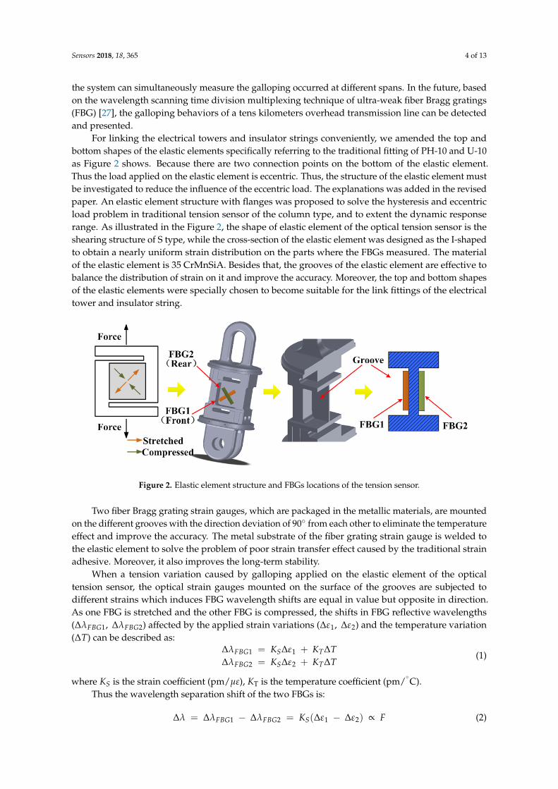
For linking the electrical towers and insulator strings conveniently, we amended the top andbottom shapes of the elastic elements specifically referring to the traditional fitting of PH-10 and U-10as Figure 2 shows. Because there are two connection points on the bottom of the elastic element.Thus the load applied on the elastic element is eccentric. Thus, the structure of the elastic element mustbe investigated to reduce the influence of the eccentric load. The explanations was added in the revisedpaper. An elastic element structure with flanges was proposed to solve the hysteresis and eccentricload problem in traditional tension sensor of the column type, and to extent the dynamic responserange. As illustrated in the Figure 2, the shape of elastic element of the optical tension sensor is theshearing structure of S type, while the cross-section of the elastic element was designed as the I-shapedto obtain a nearly uniform strain distribution on the parts where the FBGs measured. The materialof the elastic element is 35 CrMnSiA. Besides that, the grooves of the elastic element are effective tobalance the distribution of strain on it and improve the accuracy. Moreover, the top and bottom shapesof the elastic elements were specially chosen to become suitable for the link fittings of the electricaltower and insulator string.
2
Figure 2 Figure 2. Elastic element structure and FBGs locations of the tension sensor.
Two fiber Bragg grating strain gauges, which are packaged in the metallic materials, are mountedon the different grooves with the direction deviation of 90◦ from each other to eliminate the temperatureeffect and improve the accuracy. The metal substrate of the fiber grating strain gauge is welded tothe elastic element to solve the problem of poor strain transfer effect caused by the traditional strainadhesive. Moreover, it also improves the long-term stability.
When a tension variation caused by galloping applied on the elastic element of the opticaltension sensor, the optical strain gauges mounted on the surface of the grooves are subjected todifferent strains which induces FBG wavelength shifts are equal in value but opposite in direction.As one FBG is stretched and the other FBG is compressed, the shifts in FBG reflective wavelengths(∆λFBG1, ∆λFBG2) affected by the applied strain variations (∆ε1, ∆ε2) and the temperature variation(∆T) can be described as:
∆λFBG1 = KS∆ε1 + KT∆T∆λFBG2 = KS∆ε2 + KT∆T
(1)
where KS is the strain coefficient (pm/µε), KT is the temperature coefficient (pm/◦C).
Thus the wavelength separation shift of the two FBGs is:
∆λ = ∆λFBG1 − ∆λFBG2 = KS(∆ε1 − ∆ε2) ∝ F (2)
Sensors 2018, 18, 365 5 of 13
As indicated in (2), the wavelength separation shift of two FBGs is independent from thetemperature but proportional to the tension caused by galloping. The cross-sensitivity of FBGsto temperature variation is overcome by using the built-in differential structure.
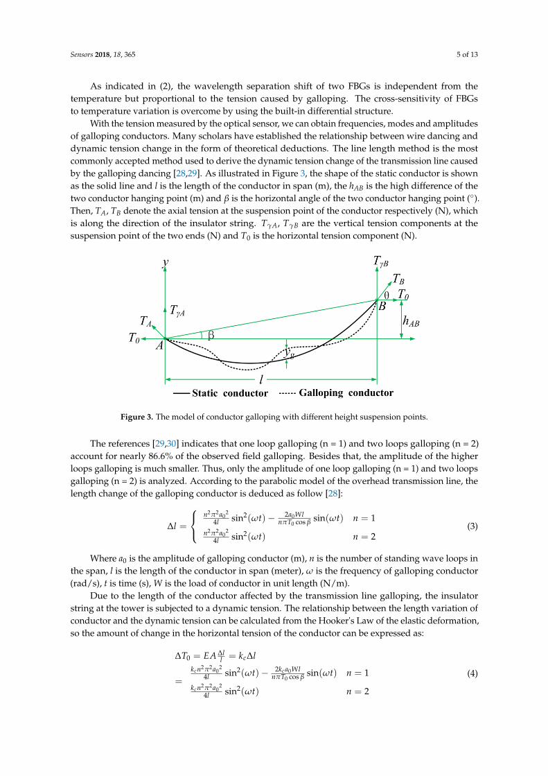
With the tension measured by the optical sensor, we can obtain frequencies, modes and amplitudesof galloping conductors. Many scholars have established the relationship between wire dancing anddynamic tension change in the form of theoretical deductions. The line length method is the mostcommonly accepted method used to derive the dynamic tension change of the transmission line causedby the galloping dancing [28,29]. As illustrated in Figure 3, the shape of the static conductor is shownas the solid line and l is the length of the conductor in span (m), the hAB is the high difference of thetwo conductor hanging point (m) and β is the horizontal angle of the two conductor hanging point (◦).Then, TA, TB denote the axial tension at the suspension point of the conductor respectively (N), whichis along the direction of the insulator string. TγA, TγB are the vertical tension components at thesuspension point of the two ends (N) and T0 is the horizontal tension component (N).
Sensors 2018, 18, 365 5 of 13
Thus the wavelength separation shift of the two FBGs is:
1 2 1 2 = FBG FBG SK F (2)
As indicated in (2), the wavelength separation shift of two FBGs is independent from the
temperature but proportional to the tension caused by galloping. The cross-sensitivity of FBGs to
temperature variation is overcome by using the built-in differential structure.
With the tension measured by the optical sensor, we can obtain frequencies, modes and
amplitudes of galloping conductors. Many scholars have established the relationship between wire
dancing and dynamic tension change in the form of theoretical deductions. The line length method
is the most commonly accepted method used to derive the dynamic tension change of the
transmission line caused by the galloping dancing [28,29]. As illustrated in Figure 3, the shape of
the static conductor is shown as the solid line and l is the length of the conductor in span (m), the
hAB is the high difference of the two conductor hanging point (m) and is the horizontal angle of the
two conductor hanging point ( ). Then, TA, TB denote the axial tension at the suspension point of
the conductor respectively (N), which is along the direction of the insulator string. TA, TB are the
vertical tension components at the suspension point of the two ends (N) and T0 is the horizontal
tension component (N).
Figure 3. The model of conductor galloping with different height suspension points.
The references [29,30] indicates that one loop galloping (n = 1) and two loops galloping (n = 2)
account for nearly 86.6% of the observed field galloping. Besides that, the amplitude of the higher
loops galloping is much smaller. Thus, only the amplitude of one loop galloping (n = 1) and two
loops galloping (n = 2) is analyzed. According to the parabolic model of the overhead transmission
line, the length change of the galloping conductor is deduced as follow [28]:
2 2 220 0
0
2 2 220
2sin ( ) sin( ) =1
4 cos
sin ( ) =24
n a a Wlt t n
l n Tl
n at n
l
(3)
Where a0 is the amplitude of galloping conductor (m), n is the number of standing wave loops
in the span, l is the length of the conductor in span (meter), is the frequency of galloping
conductor (rad/s), t is time (s), W is the load of conductor in unit length (N/m).
Due to the length of the conductor affected by the transmission line galloping, the insulator
string at the tower is subjected to a dynamic tension. The relationship between the length variation
of conductor and the dynamic tension can be calculated from the Hooker's Law of the elastic
Figure 3. The model of conductor galloping with different height suspension points.
The references [29,30] indicates that one loop galloping (n = 1) and two loops galloping (n = 2)account for nearly 86.6% of the observed field galloping. Besides that, the amplitude of the higherloops galloping is much smaller. Thus, only the amplitude of one loop galloping (n = 1) and two loopsgalloping (n = 2) is analyzed. According to the parabolic model of the overhead transmission line, thelength change of the galloping conductor is deduced as follow [28]:
∆l =
n2π2a0
2
4l sin2(ωt)− 2a0WlnπT0 cos β sin(ωt) n = 1
n2π2a02
4l sin2(ωt) n = 2(3)
Where a0 is the amplitude of galloping conductor (m), n is the number of standing wave loops inthe span, l is the length of the conductor in span (meter), ω is the frequency of galloping conductor(rad/s), t is time (s), W is the load of conductor in unit length (N/m).
Due to the length of the conductor affected by the transmission line galloping, the insulatorstring at the tower is subjected to a dynamic tension. The relationship between the length variation ofconductor and the dynamic tension can be calculated from the Hooker's Law of the elastic deformation,so the amount of change in the horizontal tension of the conductor can be expressed as:
∆T0 = EA ∆ll = kc∆l
=
kcn2π2a02
4l sin2(ωt)− 2kca0WlnπT0 cos β sin(ωt) n = 1
kcn2π2a02
4l sin2(ωt) n = 2
(4)

Sensors 2018, 18, 365 6 of 13
where kc = EA/l, E is the Young modulus of the conductor (N/mm2), A is the cross-sectional area ofthe conductor (mm2).
The amplitude is determined from the tension and Equation (4). Firstly, the parameters about thespecific transmission line is obtained from the design company or the power utility. Then, the tensionand the frequency of galloping conductor is calculated based on the sensor measurement result.
Thirdly, the number of standing wave loops can be estimated with the amplitude spectrum oftension measured. For one loop galloping (n = 1), because sin2 (ωt) = (1−cos2ωt)/2, there are twodominant oscillation frequencies in the amplitude spectrum of tension measured, and one oscillationfrequency is twice the frequency of the other (as indicated in Equation (4)). For two loops galloping(n = 2), there is only one oscillation frequency. The estimation procedure of the number of standingwave loops are also explained in the section about the experiment result. Finally, with the parametersobtained in the above three procedures, the amplitude of the galloping can be calculated based onEquation (4).
3. Dynamic Experiment of Tension Sensor
3.1. Tension Sensor Dynamic measurement
Under wind forces, phase conductors with ice may gallop. As mentioned in the Introduction, theworking range requirement of the system is 0.2–3 Hz. Obviously, a static experiment is not enoughto investigate the performance of the developed tension sensor in the field galloping monitoring.Therefore, the developed tension sensor was stretched at different frequencies using a high forceelectromechanical tester to examine the dynamic output characters. The experimental setup is shownin Figure 4.
Sensors 2018, 18, 365 6 of 13
deformation, so the amount of change in the horizontal tension of the conductor can be expressed
as:
0
2 2 220 0
0
2 2 220
2sin ( ) sin( ) =1
4 cos
sin ( ) =24
c
c c
c
lT EA k l
l
k n a k a Wlt t n
l n T
k n at n
l
(4)
where kc = EA/l, E is the Young modulus of the conductor (N/mm2), A is the cross-sectional area of
the conductor (mm2).
The amplitude is determined from the tension and Equation (4). Firstly, the parameters about
the specific transmission line is obtained from the design company or the power utility. Then, the
tension and the frequency of galloping conductor is calculated based on the sensor measurement
result.
Thirdly, the number of standing wave loops can be estimated with the amplitude spectrum of
tension measured. For one loop galloping (n = 1), because sin2 (t) = (1cos2t)/2, there are two
dominant oscillation frequencies in the amplitude spectrum of tension measured, and one
oscillation frequency is twice the frequency of the other (as indicated in Equation (4)). For two loops
galloping (n = 2), there is only one oscillation frequency. The estimation procedure of the number of
standing wave loops are also explained in the section about the experiment result. Finally, with the
parameters obtained in the above three procedures, the amplitude of the galloping can be
calculated based on Equation (4).
3. Dynamic Experiment of Tension Sensor
3.1. Tension Sensor Dynamic measurement
Under wind forces, phase conductors with ice may gallop. As mentioned in the Introduction,
the working range requirement of the system is 0.2–3 Hz. Obviously, a static experiment is not
enough to investigate the performance of the developed tension sensor in the field galloping
monitoring. Therefore, the developed tension sensor was stretched at different frequencies using a
high force electromechanical tester to examine the dynamic output characters. The experimental
setup is shown in Figure 4.
(a) The overall layout of the experiment (b) The tension sensor installation
Figure 4. The setup of the dynamic stretched experiment. Figure 4. The setup of the dynamic stretched experiment.
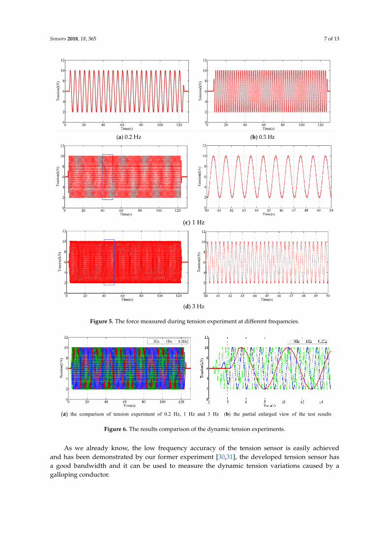
The proposed sensor was stretched in the form of sinusoidal waves at the frequencies from 0.2 Hzto 3 Hz, using the force amplitudes from 2 kN to 10 kN. The tension experiment at different singlefrequency lasted for 2 min. The tensions measured during the experiments at the different frequenciesare shown in Figures 5 and 6. The results of the experiments indicate that the output of the developedtension sensor is stable in the frequency range 0.2 Hz to 3 Hz.
Sensors 2018, 18, 365 7 of 13
Sensors 2018, 18, 365 7 of 13
The proposed sensor was stretched in the form of sinusoidal waves at the frequencies from 0.2
Hz to 3 Hz, using the force amplitudes from 2 kN to 10 kN. The tension experiment at different
single frequency lasted for 2 min. The tensions measured during the experiments at the different
frequencies are shown in Figures 5 and 6. The results of the experiments indicate that the output of
the developed tension sensor is stable in the frequency range 0.2 Hz to 3 Hz.
(a) 0.2 Hz (b) 0.5 Hz
(c) 1 Hz
(d) 3 Hz
Figure 5. The force measured during tension experiment at different frequencies.
(a) the comparison of tension experiment of 0.2 Hz, 1 Hz and 3 Hz (b) the partial enlarged view of the test results
Figure 6. The results comparison of the dynamic tension experiments.
As we already know, the low frequency accuracy of the tension sensor is easily achieved and
has been demonstrated by our former experiment [30,31], the developed tension sensor has a good
bandwidth and it can be used to measure the dynamic tension variations caused by a galloping
conductor.
Figure 5. The force measured during tension experiment at different frequencies.
Sensors 2016, 16, x 7 of 13
The proposed sensor was stretched in the form of sinusoidal waves at the frequencies from 0.2 Hz to 3 Hz, using the force amplitudes from 2 kN to 10 kN. The tension experiment at different single frequency lasted for 2 min. The tensions measured during the experiments at the different frequencies are shown in Figures 5 and 6. The results of the experiments indicate that the output of the developed tension sensor is stable in the frequency range 0.2 Hz to 3 Hz.
(a) 0.2 Hz (b) 0.5 Hz
(c) 1 Hz
(d) 3 Hz
Figure 5. The force measured during tension experiment at different frequencies.
(a) the comparison of tension experiment of 0.2 Hz, 1 Hz and 3 Hz (b) the partial enlarged view of the test results
Figure 6. The results comparison of the dynamic tension experiments.
As we already know, the low frequency accuracy of the tension sensor is easily achieved and has been demonstrated by our former experiment [30,31], the developed tension sensor has a good bandwidth and it can be used to measure the dynamic tension variations caused by a galloping conductor.
Figure 6. The results comparison of the dynamic tension experiments.
As we already know, the low frequency accuracy of the tension sensor is easily achievedand has been demonstrated by our former experiment [30,31], the developed tension sensor hasa good bandwidth and it can be used to measure the dynamic tension variations caused by agalloping conductor.
Sensors 2018, 18, 365 8 of 13
3.2. Tension Sensor Fatigue Experiment
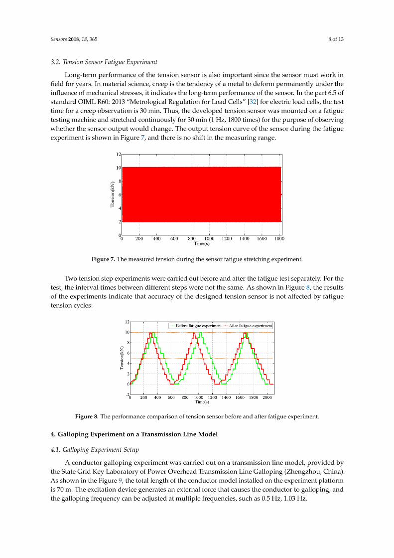
Long-term performance of the tension sensor is also important since the sensor must work infield for years. In material science, creep is the tendency of a metal to deform permanently under theinfluence of mechanical stresses, it indicates the long-term performance of the sensor. In the part 6.5 ofstandard OIML R60: 2013 “Metrological Regulation for Load Cells” [32] for electric load cells, the testtime for a creep observation is 30 min. Thus, the developed tension sensor was mounted on a fatiguetesting machine and stretched continuously for 30 min (1 Hz, 1800 times) for the purpose of observingwhether the sensor output would change. The output tension curve of the sensor during the fatigueexperiment is shown in Figure 7, and there is no shift in the measuring range.
Sensors 2018, 18, 365 8 of 13
3.2. Tension Sensor Fatigue Experiment
Long-term performance of the tension sensor is also important since the sensor must work in
field for years. In material science, creep is the tendency of a metal to deform permanently under
the influence of mechanical stresses, it indicates the long-term performance of the sensor. In the part
6.5 of standard OIML R60: 2013 “Metrological Regulation for Load Cells” [32] for electric load cells,
the test time for a creep observation is 30 min. Thus, the developed tension sensor was mounted on
a fatigue testing machine and stretched continuously for 30 min (1 Hz, 1800 times) for the purpose
of observing whether the sensor output would change. The output tension curve of the sensor
during the fatigue experiment is shown in Figure 7, and there is no shift in the measuring range.
Two tension step experiments were carried out before and after the fatigue test separately. For
the test, the interval times between different steps were not the same. As shown in Figure 8, the
results of the experiments indicate that accuracy of the designed tension sensor is not affected by
fatigue tension cycles.
Figure 7. The measured tension during the sensor fatigue stretching experiment.
Figure 8. The performance comparison of tension sensor before and after fatigue experiment.
4. Galloping Experiment on a Transmission Line Model
4.1. Galloping Experiment Setup
A conductor galloping experiment was carried out on a transmission line model, provided by
the State Grid Key Laboratory of Power Overhead Transmission Line Galloping (Zhengzhou,
China). As shown in the Figure 9, the total length of the conductor model installed on the
experiment platform is 70 m. The excitation device generates an external force that causes the
conductor to galloping, and the galloping frequency can be adjusted at multiple frequencies, such
as 0.5 Hz, 1.03 Hz.
Figure 7. The measured tension during the sensor fatigue stretching experiment.
Two tension step experiments were carried out before and after the fatigue test separately. For thetest, the interval times between different steps were not the same. As shown in Figure 8, the resultsof the experiments indicate that accuracy of the designed tension sensor is not affected by fatiguetension cycles.
Sensors 2018, 18, 365 8 of 13
3.2. Tension Sensor Fatigue Experiment
Long-term performance of the tension sensor is also important since the sensor must work in
field for years. In material science, creep is the tendency of a metal to deform permanently under
the influence of mechanical stresses, it indicates the long-term performance of the sensor. In the part
6.5 of standard OIML R60: 2013 “Metrological Regulation for Load Cells” [32] for electric load cells,
the test time for a creep observation is 30 min. Thus, the developed tension sensor was mounted on
a fatigue testing machine and stretched continuously for 30 min (1 Hz, 1800 times) for the purpose
of observing whether the sensor output would change. The output tension curve of the sensor
during the fatigue experiment is shown in Figure 7, and there is no shift in the measuring range.
Two tension step experiments were carried out before and after the fatigue test separately. For
the test, the interval times between different steps were not the same. As shown in Figure 8, the
results of the experiments indicate that accuracy of the designed tension sensor is not affected by
fatigue tension cycles.
Figure 7. The measured tension during the sensor fatigue stretching experiment.
Figure 8. The performance comparison of tension sensor before and after fatigue experiment.
4. Galloping Experiment on a Transmission Line Model
4.1. Galloping Experiment Setup
A conductor galloping experiment was carried out on a transmission line model, provided by
the State Grid Key Laboratory of Power Overhead Transmission Line Galloping (Zhengzhou,
China). As shown in the Figure 9, the total length of the conductor model installed on the
experiment platform is 70 m. The excitation device generates an external force that causes the
conductor to galloping, and the galloping frequency can be adjusted at multiple frequencies, such
as 0.5 Hz, 1.03 Hz.
Figure 8. The performance comparison of tension sensor before and after fatigue experiment.
4. Galloping Experiment on a Transmission Line Model
4.1. Galloping Experiment Setup
A conductor galloping experiment was carried out on a transmission line model, provided bythe State Grid Key Laboratory of Power Overhead Transmission Line Galloping (Zhengzhou, China).As shown in the Figure 9, the total length of the conductor model installed on the experiment platformis 70 m. The excitation device generates an external force that causes the conductor to galloping, andthe galloping frequency can be adjusted at multiple frequencies, such as 0.5 Hz, 1.03 Hz.

Sensors 2018, 18, 365 9 of 13Sensors 2018, 18, 365 9 of 13
Figure 9. The setup of galloping experiment on transmission line model.
During the experiment, the horizontal dynamic tensions produced by the transmission line
model galloping were recorded by an electronic tension sensor and the optical tension sensor. We
installed the optical tension sensor at one end of the transmission line model, which was connected
in series with the electronic tension sensor, which are illustrated in Figure 10. The sampling
frequency in the experiment was set to 20 Hz.
Figure 10. The connection diagram of tension sensors.
4.2. Experiment Results and Discussion
At the beginning of the galloping experiment, we recorded the initial wavelengths of the
optical strain gauges mounted on the tension sensor, which were 1554.983 pm and 1549.889 pm.
Then, the experiment platform was powered to make the transmission line model galloping.
Experience shows that the inherent resonant frequency of the OHTL model is near 1 Hz, below
which the conductor is prone to large-scale galloping. Thus, in the first test, the drive frequency of
the experiment platform was set to 1.02 Hz. The whole process of the first galloping test included
two procedures of start and stop, the tension is plotted in Figures 11 and 12.
As shown in Figure 12, the output of the optical tension sensor is basically consistent with that
of the electronic tension sensor, which proves that the optical tension sensor has good dynamic
measurement characteristics.
The fast Fourier transform (FFT) was applied to obtain the amplitude spectrum of tension
measured. Figure 13 indicates that the dominant oscillation frequency is near 1 Hz, which is
consistent with the drive frequency set in the experiment. The frequency is close to the natural
oscillation frequency of the experimental transmission line model.
Figure 9. The setup of galloping experiment on transmission line model.
During the experiment, the horizontal dynamic tensions produced by the transmission line modelgalloping were recorded by an electronic tension sensor and the optical tension sensor. We installedthe optical tension sensor at one end of the transmission line model, which was connected in serieswith the electronic tension sensor, which are illustrated in Figure 10. The sampling frequency in theexperiment was set to 20 Hz.
Sensors 2018, 18, 365 9 of 13
Figure 9. The setup of galloping experiment on transmission line model.
During the experiment, the horizontal dynamic tensions produced by the transmission line
model galloping were recorded by an electronic tension sensor and the optical tension sensor. We
installed the optical tension sensor at one end of the transmission line model, which was connected
in series with the electronic tension sensor, which are illustrated in Figure 10. The sampling
frequency in the experiment was set to 20 Hz.
Figure 10. The connection diagram of tension sensors.
4.2. Experiment Results and Discussion
At the beginning of the galloping experiment, we recorded the initial wavelengths of the
optical strain gauges mounted on the tension sensor, which were 1554.983 pm and 1549.889 pm.
Then, the experiment platform was powered to make the transmission line model galloping.
Experience shows that the inherent resonant frequency of the OHTL model is near 1 Hz, below
which the conductor is prone to large-scale galloping. Thus, in the first test, the drive frequency of
the experiment platform was set to 1.02 Hz. The whole process of the first galloping test included
two procedures of start and stop, the tension is plotted in Figures 11 and 12.
As shown in Figure 12, the output of the optical tension sensor is basically consistent with that
of the electronic tension sensor, which proves that the optical tension sensor has good dynamic
measurement characteristics.
The fast Fourier transform (FFT) was applied to obtain the amplitude spectrum of tension
measured. Figure 13 indicates that the dominant oscillation frequency is near 1 Hz, which is
consistent with the drive frequency set in the experiment. The frequency is close to the natural
oscillation frequency of the experimental transmission line model.
Figure 10. The connection diagram of tension sensors.
4.2. Experiment Results and Discussion
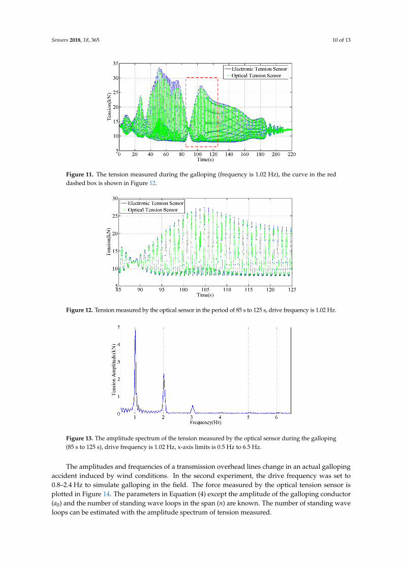
At the beginning of the galloping experiment, we recorded the initial wavelengths of the opticalstrain gauges mounted on the tension sensor, which were 1554.983 pm and 1549.889 pm. Then, theexperiment platform was powered to make the transmission line model galloping. Experience showsthat the inherent resonant frequency of the OHTL model is near 1 Hz, below which the conductor isprone to large-scale galloping. Thus, in the first test, the drive frequency of the experiment platformwas set to 1.02 Hz. The whole process of the first galloping test included two procedures of start andstop, the tension is plotted in Figures 11 and 12.
As shown in Figure 12, the output of the optical tension sensor is basically consistent withthat of the electronic tension sensor, which proves that the optical tension sensor has good dynamicmeasurement characteristics.
The fast Fourier transform (FFT) was applied to obtain the amplitude spectrum of tensionmeasured. Figure 13 indicates that the dominant oscillation frequency is near 1 Hz, which is consistentwith the drive frequency set in the experiment. The frequency is close to the natural oscillationfrequency of the experimental transmission line model.
Sensors 2018, 18, 365 10 of 13
3
Figure 11 Figure 11. The tension measured during the galloping (frequency is 1.02 Hz), the curve in the red
dashed box is shown in Figure 12.
4
Figure 12 Figure 12. Tension measured by the optical sensor in the period of 85 s to 125 s, drive frequency is 1.02 Hz.
Sensors 2018, 18, 365 10 of 13
Figure 11. The tension measured during the galloping (frequency is 1.02 Hz), the curve in the red
dashed box is shown in Figure 12.
Figure 12. Tension measured by the optical sensor in the period of 85 s to 125 s, drive frequency is
1.02 Hz.
Figure 13. The amplitude spectrum of the tension measured by the optical sensor during the
galloping (85 s to 125 s), drive frequency is 1.02 Hz, x-axis limits is 0.5 Hz to 6.5 Hz.
The amplitudes and frequencies of a transmission overhead lines change in an actual galloping
accident induced by wind conditions. In the second experiment, the drive frequency was set to
0.8–2.4 Hz to simulate galloping in the field. The force measured by the optical tension sensor is
plotted in Figure 14. The parameters in Equation (4) except the amplitude of the galloping
Figure 13. The amplitude spectrum of the tension measured by the optical sensor during the galloping(85 s to 125 s), drive frequency is 1.02 Hz, x-axis limits is 0.5 Hz to 6.5 Hz.
The amplitudes and frequencies of a transmission overhead lines change in an actual gallopingaccident induced by wind conditions. In the second experiment, the drive frequency was set to0.8–2.4 Hz to simulate galloping in the field. The force measured by the optical tension sensor isplotted in Figure 14. The parameters in Equation (4) except the amplitude of the galloping conductor(a0) and the number of standing wave loops in the span (n) are known. The number of standing waveloops can be estimated with the amplitude spectrum of tension measured.

Sensors 2018, 18, 365 11 of 13
Zoomed tensions and their amplitude spectrums are illustrated in the Figure 15. Between 130 s to150 s, the force measured and its amplitude spectrum are shown in Figure 15a. There are two dominantoscillation frequencies, 1 Hz and 2 Hz, in the measured amplitude spectrum of the tension, and oneoscillation frequency (2 Hz) is twice the frequency of the other (1 Hz). According to the analysis before,it is a one loop galloping, n = 1.
Between 290 s to 295 s, the force measured and its amplitude spectrum are shown in Figure 15b.There is only one oscillation frequency span, According to the analysis before, it is a two loopsgalloping, n = 2.
The standing wave loops estimation procedures are illustrated by the video provided in theSupplementary Material of this manuscript, 15 s (n = 1) and 50 s (n = 2).
The developed optical tension sensor can accurately distinguish the characteristic frequencyand mode of the conductor galloping, the amplitude can be determined from the tension based onEquation (4). The performance of the developed sensor is demonstrated by the dynamic measurements.
Sensors 2018, 18, 365 11 of 13
conductor (a0) and the number of standing wave loops in the span (n) are known. The number of
standing wave loops can be estimated with the amplitude spectrum of tension measured.
Zoomed tensions and their amplitude spectrums are illustrated in the Figure 15. Between 130 s
to 150 s, the force measured and its amplitude spectrum are shown in Figure 15a. There are two
dominant oscillation frequencies, 1 Hz and 2 Hz, in the measured amplitude spectrum of the
tension, and one oscillation frequency (2 Hz) is twice the frequency of the other (1 Hz). According
to the analysis before, it is a one loop galloping, n = 1.
Between 290 s to 295 s, the force measured and its amplitude spectrum are shown in Figure 15b.
There is only one oscillation frequency span, According to the analysis before, it is a two loops
galloping, n = 2.
The standing wave loops estimation procedures are illustrated by the video provided in the
Supplementary Material of this manuscript, 15 s (n = 1) and 50 s (n = 2).
The developed optical tension sensor can accurately distinguish the characteristic frequency
and mode of the conductor galloping, the amplitude can be determined from the tension based on
Equation (4). The performance of the developed sensor is demonstrated by the dynamic
measurements.
Figure 14. The dynamic tension results in the second galloping experiment, in which different drive
frequencies were used.
(a) Between 130 s to 150 s.
(b) Between 290 s to 295 s.
Figure 15. Measured tension and its amplitude spectrum (x-axis limits is 0.5 Hz to 6.5 Hz) during
the galloping frequency variation experiment.
Figure 14. The dynamic tension results in the second galloping experiment, in which different drivefrequencies were used.
Sensors 2018, 18, 365 11 of 13
conductor (a0) and the number of standing wave loops in the span (n) are known. The number of
standing wave loops can be estimated with the amplitude spectrum of tension measured.
Zoomed tensions and their amplitude spectrums are illustrated in the Figure 15. Between 130 s
to 150 s, the force measured and its amplitude spectrum are shown in Figure 15a. There are two
dominant oscillation frequencies, 1 Hz and 2 Hz, in the measured amplitude spectrum of the
tension, and one oscillation frequency (2 Hz) is twice the frequency of the other (1 Hz). According
to the analysis before, it is a one loop galloping, n = 1.
Between 290 s to 295 s, the force measured and its amplitude spectrum are shown in Figure 15b.
There is only one oscillation frequency span, According to the analysis before, it is a two loops
galloping, n = 2.
The standing wave loops estimation procedures are illustrated by the video provided in the
Supplementary Material of this manuscript, 15 s (n = 1) and 50 s (n = 2).
The developed optical tension sensor can accurately distinguish the characteristic frequency
and mode of the conductor galloping, the amplitude can be determined from the tension based on
Equation (4). The performance of the developed sensor is demonstrated by the dynamic
measurements.
Figure 14. The dynamic tension results in the second galloping experiment, in which different drive
frequencies were used.
(a) Between 130 s to 150 s.
(b) Between 290 s to 295 s.
Figure 15. Measured tension and its amplitude spectrum (x-axis limits is 0.5 Hz to 6.5 Hz) during
the galloping frequency variation experiment. Figure 15. Measured tension and its amplitude spectrum (x-axis limits is 0.5 Hz to 6.5 Hz) during thegalloping frequency variation experiment.
Sensors 2018, 18, 365 12 of 13
5. Conclusions
A novel optical passive measuring system is proposed for monitoring the galloping of overheadtransmission lines by using the OPGW transmission. The benefits of the optical detection method areanti-electromagnetic interference, no power supply requirement and long life in humid environments.
An ‘S’ type elastic element structure with flanges is proposed to solve the hysteresis and eccentricload problems, and to extent the dynamic response range. The tension experiments carried outusing a high force electromechanical tester demonstrate the dynamic response characteristics. Fatigueexperiments verified the long term stability of the sensor.
To examine the feasibility of the proposed on-line monitoring system operated on a phaseconductor, different patterns galloping were generated in a 70 m conductor model, and theexperimental results demonstrated that the sensor is suitable for OHTL galloping detection.
Compared with the optical sensors for OHTL monitoring, the system has many advantages,such as easy installation, no flashover risk, distribution monitoring, better bandwidth, improvedaccuracy and higher reliability.
Supplementary Materials: The supplementary materials are available online at www.mdpi.com/1424-8220/18/02/365/s1.
Acknowledgments: This work was supported in part by National Natural Science Foundation of China (GrantNo. 51677070), Beijing Natural Science Foundation (3182036), Fundamental Research Funds for the CentralUniversities (JB2015RCY02), “111” Project (B08013) and Young Elite Scientists Sponsorship Program by CAST.
Author Contributions: Guo-ming Ma and Cheng-rong Li conceived and designed the experiments; Nai-qiang Mao,Ya-bo Li, Cheng Shi and Bo Zhang performed the experiments; Guo-ming Ma and Nai-qiang Mao analyzed the data;Guo-ming Ma, Ya-bo Li and Nai-qiang Mao wrote the paper.
Conflicts of Interest: The authors declare no conflict of interest.
References
1. CIGRE Working Group B2.29. Systems for Prediction and Monitoring of Ice Shedding, Anti-Icing and De-Icing forOverhead Lines (TB 438); CIGRE: Paris, France, 2010; pp. 9–15.
2. CIGRE Working Group B2.06. Big Storm Events-What We Have Learned (TB 344); CIGRE: Paris, France, 2008;pp. 52–56.
3. CIGRE Technical Brochure B2.11.06. State of The Art of Conductor Galloping (TB 322); CIGRE: Paris, France,2007; pp. 29–74.
4. Douglass, D.; Chisholm, W.; Davidson, G.; Grant, I.; Lindsey, K.; Lancaster, M.; Lawry, D.; McCarthy, T.;Nascimento, C.; Pasha, M.; et al. Real-time overhead transmission-line monitoring for dynamic rating.IEEE Trans. Power Deliv. 2016, 31, 921–927. [CrossRef]
5. Zangl, H.; Bretterklieber, T; Brasseur, G. A feasibility study on autonomous online condition monitoring ofhigh-voltage overhead power lines. IEEE Trans. Instrum. Meas. 2009, 58, 1789–1796. [CrossRef]
6. De Paulis, F.; Olivieri, C.; Orlandi, A.; Giannuzzi, G. Detectability of degraded joint discontinuities in HVpower lines through TDR-like remote monitoring. IEEE Trans. Instrum. Meas. 2016, 12, 2725–2733. [CrossRef]
7. De Paulis, F.; Olivieri, C.; Orlandi, A.; Giannuzzi, G.; Bassi, F.; Morandini, C.; Fiorucci, E.; Bucci, G. Exploringremote monitoring of degraded compression and bolted joints in HV power transmission lines. IEEE Trans.Power Deliv. 2016, 5, 2179–2187. [CrossRef]
8. Farzaneh, M. Ice accretions on high–voltage conductors and insulators and related phenomena. Philos. Trans.A Math. Phys. Eng. Sci. 2000, 358, 2971–3005. [CrossRef]
9. Nigol, O.; Buchan, P.G. Conductor Galloping Part I: Den Hartog Mechanism. IEEE Trans. Power App. Syst.1981, 100, 699–707. [CrossRef]
10. Lu, M.L.; Popplewell, N.; Shah, A.H.; Chan, J.K. Hybrid Nutation Damper for Controlling Galloping PowerLines. IEEE Trans. Power Deliv. 2007, 22, 450–456. [CrossRef]
11. Wang, J.; Lilien, J.-L. Overhead electrical transmission line galloping: A full multi-span 3-DOF model, someapplications and design recommendations. IEEE Trans. Power Deliv. 1998, 13, 909–916. [CrossRef]
12. Dyke, P.V.; Laneville, A. Galloping of a single conductor covered with a D-section on a high-voltage overheadtest line. J. Wind Eng. Ind. Aerod. 2008, 96, 1141–1151. [CrossRef]

Sensors 2018, 18, 365 13 of 13
13. Stephen, J.M. Fiber Bragg Grating Sensors for Harsh Environments. Sensors 2012, 12, 1898–1918. [CrossRef]14. Lilien, J.; Erpicum, M.; Wolfs, M. Overhead line galloping. Field experience during one event in Belgium on
last February 13th, 1997. Atmos. Icing Struct. 1998, 293–299. [CrossRef]15. Weraneck, K.; Heilmeier, F.; Lindner, M.; Graf, M.; Jakobi, M.; Volk, W.; Boths, J.; Koch, A.W. Strain
Measurement in Aluminium Alloy during the Solidification Process Using Embedded Fibre Bragg Gratings.Sensors 2016, 16, 1853. [CrossRef] [PubMed]
16. Wang, J.; Zhao, L.; Liu, T.; Li, Z.; Sun, T.; Grattan, K.T.V. Novel Negative Pressure Wave-based Pipeline LeakDetection System Using Fiber Bragg Grating-based Pressure Sensors. J. Lightwave Technol. 2017, 35, 3366–3373.[CrossRef]
17. Zhang, Q.; Wang, Y.; Sun, Y.; Gao, L.; Zhang, Z.; Zhang, W.; Zhao, P.; Yue, Y. Using custom fiber Bragggrating-based sensors to monitor artificial landslides. Sensors 2016, 16, 1417. [CrossRef] [PubMed]
18. Ma, G.; Li, C.; Luo, Y.; Mu, R.; Wang, L. High sensitive and reliable fiber Bragg grating hydrogen sensor forfault detection of power transformer. Sens. Actuat. B-Chem. 2012, 169, 195–198. [CrossRef]
19. Guo, T. Fiber Grating Assisted Surface Plasmon Resonance for Biochemical and Electrochemical Sensing.J. Lightwave Technol. 2017, 35, 3323–3333. [CrossRef]
20. Song, X.; Zhang, Y.; Liang, D. Load Identification for a Cantilever Beam Based on Fiber Bragg GratingSensors. Sensors 2017, 17, 1733. [CrossRef] [PubMed]
21. Ma, G.; Li, C.; Jiang, J.; Liang, J.; Luo, Y.; Cheng, Y. A passive optical fiber anemometer for wind speedmeasurement on high-voltage overhead transmission lines. IEEE Trans. Instrum. Meas. 2012, 2, 539–544.[CrossRef]
22. Bjerkan, L. Application of fiber-optic bragg grating sensors in monitoring environmental loads of overheadpower transmission lines. Appl. Opt. 2000, 39, 554–560. [CrossRef] [PubMed]
23. Huang, Q.; Zhang, C.H.; Liu, Q.Y.; Ning, Y.; Cao, Y.X. New type of fiber optic sensor network for smart gridinterface of transmission system. In Proceedings of the 2010 IEEE in Power and Energy Society GeneralMeeting, Providence, RI, USA, 25–29 July 2010; pp. 1–5. [CrossRef]
24. Luo, J.B.; Hao, Y.P.; Ye, Q.; Hao, Y.Q.; Li, L.C. Development of Optical Fiber Sensors Based on BrillouinScattering and FBG for On-Line Monitoring in Overhead Transmission Lines. J. Lightwave Technol. 2013,31, 1559–1565. [CrossRef]
25. China Central Television. Video of an Overhead Line Transmission Line Maintained without Power off.Available online: https://www.youtube.com/watch?v=PHVwPwwkud8 (accessed on 17 November 2011).
26. Zhou, L.; Yan, B.; Zhang, L.; Zhou, S. Study on galloping behavior of iced eight bundle conductortransmission lines. J. Sound Vib. 2016, 362, 85–110. [CrossRef]
27. Wang, Y.; Gong, J.; Dong, B.; Wang, D.Y.; Shillig, J.; Wang, A. A Large Serial Time-Division Multiplexed FiberBragg Grating Sensor Network. J. Lightwave Technol. 2012, 30, 2751–2756. [CrossRef]
28. Wang, S.H.; Jiang, X.L.; Sun, C.X. Characteristics of Icing Conductor Galloping and Induced Dynamic TensileForce of the Conductor. Trans. China Electrotech. Soc. 2010, 25, 159–166.
29. Baenziger, M.A.; James, W.D.; Wouters, B.; Li, L. Dynamic loads on transmission line structures due togalloping conductors. IEEE Trans. Power Deliv. 1994, 9, 40–49. [CrossRef]
30. Rawlins, C.B. Analysis of conductor galloping field observations-single conductors. IEEE Trans. PowerAppar. Syst. 1981, 8, 3744–3753. [CrossRef]
31. Ma, G.; Li, C.; Quan, J.; Jiang, J.; Cheng, Y. A fiber Bragg grating tension and tilt sensor applied to icingmonitoring on overhead transmission lines. IEEE Trans. Power Deliv. 2011, 4, 2163–2170. [CrossRef]
32. OIML TC 9. Metrological Regulation for Load Cells; International Organisation of Legal Metrology: Lindfield,Australia, 2013.
© 2018 by the authors. Licensee MDPI, Basel, Switzerland. This article is an open accessarticle distributed under the terms and conditions of the Creative Commons Attribution(CC BY) license (http://creativecommons.org/licenses/by/4.0/).