a few data on the calculation of beam-column joints … · 2018-01-19 · and column and joints as...

\

Acta Technica Napocensis: Civil Engineering & Architecture Volume 60, No. 2, (2017)

Journal homepage: http://constructii.utcluj.ro/ActaCivilEng

ISSN 1221-5848

A Few Data on the Calculation of Beam-Column Joints of Moment

Resisting Frames by the Methods of “Theory of Elasticity” (I)

Liviu H. CUCU*1, Ironim MARŢIAN

2, Daniel I. SUCIU

3

1,2,3Technical University of Cluj-Napoca, Faculty of Civil Engineering.

28 Memorandumului Str., 400114, Cluj-Napoca, Romania

(Received 2 May 2017; Accepted 24 December 2017)

Abstract

In this paper, the authors aim to analyze the state of stress in the beam-column joints of moment

resisting frames by accepting two cases: joints as intersection of two bars (frame corners), beam

and column and joints as intersection of three bars, two collinear columns and a beam, the latter

case being possible to be extended to the joints created as intersection of a column and two

collinear beams. The first case has been analyzed either in the “Strength of materials”, or in the

“Theory of elasticity” as a plane problem in polar coordinates. In the second case, two variants

have been taken into consideration: the beam transmits only bending moment and the beam

transmits both bending moment and shear force. In both variants, the state of plane stress that

results in the beam-column joint of the moment resisting frame has been analytically determined

based on the stress formulation, depending on the ratio of the height of the column cross section

to that of the beam. In this way, the state of stress provided in the works [2] and [5] has been

corrected.

Rezumat

În prezenta lucrare, autorii îşi propun să analizeze starea de tensiune în nodurile de cadre

acceptând două cazuri: noduri ca intersecţie a două bare (colţuri de cadre), montant (stâlp) şi

riglă, şi noduri ca intersecţie a trei bare, doi montanţi în prelungire şi riglă, acest din urmă caz

fiind posibil de extins şi la nodurile ca intersecţie a unui montant şi două rigle în prelungire.

Primul caz este tratat fie în „Rezistenţa materialelor”, fie în „Teoria elasticităţii”, ca problemă

plană în coordonate polare. În al doilea caz, se consideră două variante: rigla transmite numai

moment încovoietor şi rigla transmite atât moment încovoietor, cât şi forţă tăietoare. În ambele

variante, starea de tensiune plană care se naşte în nodul de cadru se determină analitic pe baza

formulării în tensiuni, în funcţie de raportul dintre înălţimea secţiunii montantului şi cea a riglei.

În acest fel, se corectează stările de tensiune date în lucrările [2] şi [5].

Keywords: beam-column joint, joint calculation, stress function, state of plane stress

* Corresponding author: Tel./ Fax.: 0722-878769

E-mail address: [email protected]

Cucu L.H. et al. / Acta Technica Napocensis: Civil Engineering & Architecture Vol. 60 No 2 (2017) 46-60

47

1. Overview

In the process of calculating and performing the connections between the beams and the columns of

multi-storey reinforced concrete or steel moment resisting frames, but also in the case of short

cantilevers, a special attention must be paid to the joints. In terms of calculations, the state of stress

of these joints is complex and will be determined by the methods of “Theory of elasticity”, based on

the accepted fundamental hypotheses, then the way in which the stresses are dispersed (principal

stress trajectories) from the beams to the columns (and vice-versa) is established, in the idea of a

proper member reinforcement. Usually, the joints are rigid points, which ensure the kinematic

stability, especially in the case of the frames, consisting only of beams and columns. From the

practical point of view, in order to obtain a proper beam-column connection, a part of the beam’s

reinforcement must be inserted in the column and a part of the column’s reinforcement must be

inserted into the beam. Thus, agglomerations of reinforcing bars can be produced in the beam-

column joints, which may lead to inappropriate concreting. Generally, a good detailing of the beam-

column joint consists of ensuring appropriate anchorage lengths, avoiding stress concentrations by

using haunched connections and easy concreting of these joints [1].

The determination of internal forces on the adjacent bars, which become actions on the beam-

column joints, has been done by the “Structural Analysis” methods, depending on the type of the

structure (determinate or indeterminate), mainly by imposing compatibility conditions of

deformations, eliminating the rigid body displacements in the first case and obtaining the unknown

reactions in the second case.

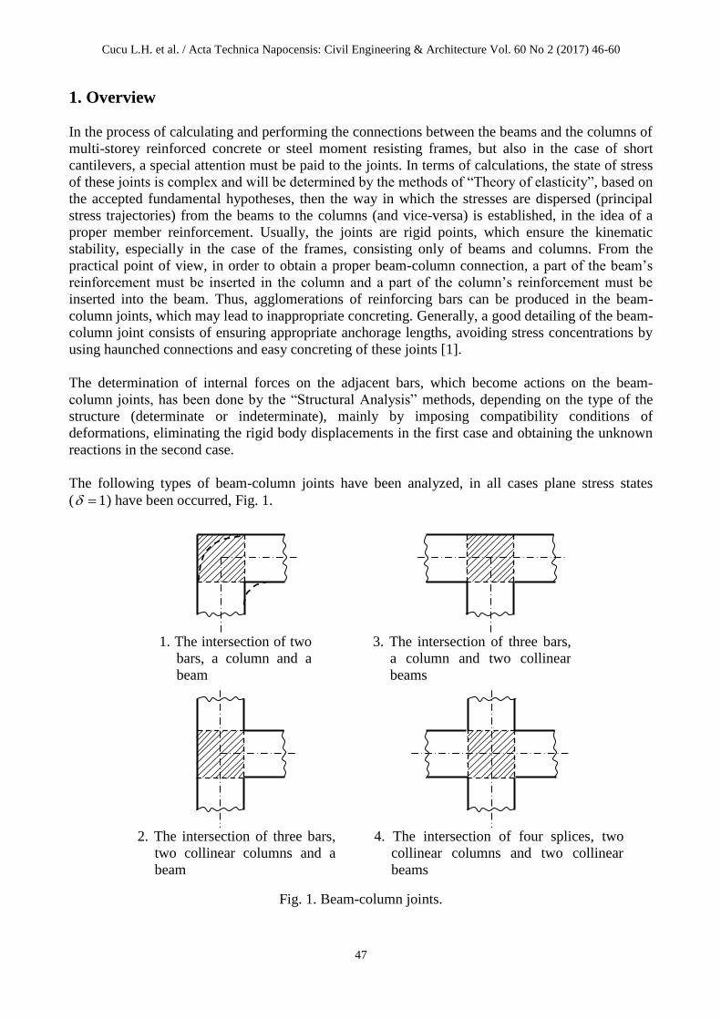
The following types of beam-column joints have been analyzed, in all cases plane stress states

( 1 ) have been occurred, Fig. 1.

Fig. 1. Beam-column joints.

1. The intersection of two

bars, a column and a

beam

2. The intersection of three bars,

two collinear columns and a

beam

3. The intersection of three bars,

a column and two collinear

beams

4. The intersection of four splices, two

collinear columns and two collinear

beams


48

2. The simple beam-column joint of moment resisting frames

In the first case (1), the state of stress can be determined, for example, from 0M (pure bending),

considered positively (tends to increase the radius of curvature), by the methods of “Strength of

materials”, accepting the validity of Bernoulli hypothesis, assuming instead of the joint a circular

curved bar with large curvature (small radius of curvature), using the relationship

yR

y

S

M

oz 0 , (1)

where is the normal stress at any point on the cross-sectional area situated at a distance y from

the neutral axis, oR is the neutral fiber’s radius of curvature, zS is the first moment of area about the

neutral axis; based on the “Theory of elasticity”, in polar coordinates, the state of stress that is

independent from the angle and the material continuously undistributed around the pole, with the

help of the relationships

,lnlnln4

;lnlnln4

2222

2

22

0

22

2

22

0

abr

aa

b

rb

r

ba

a

b

t

M

r

aa

b

rb

r

ba

a

b

t

Mr

(2)

where r is the radial stress (tensile stress), is the hoop stress on the cross section of the

circular curve bar; a is the radius of the internal side fiber and b is the radius of the external side

fiber, with the following notation:

2

22222 ln4

a

bbaabt .

For the particular case ab 2 , the extreme normal stresses given by relationships (1) and (2) are

acceptable within ±5% limits. The diagrams of r and are shown in Fig. 2 [3], [4].

Fig. 2. The diagrams of r and for the case ab 2 .

Multiplicator 2

0

a

M

7,75525

4,91702

0,64458

1,06986

r

b

a

O

2

ba

1,35955a

0M

0M


49

3. Two variants for the intersection of three bars in the beam-columns joints In the second case (2), two variants are considered: I. the beam transmits only bending

moment bPM 20 , which determines in the column the shear forces P (Fig. 3,a) ; II. the beam

transmits both bending moment 0M and shear force P , which leads to the tensile axial force P in

the column; thus, the bending moment in the beam will be PaM 0 , while the internal forces in the

column will be PT 3 and PaM 2 , where b

a , a and b being the dimensions of the joint

considered as a rectangular diaphragm (Fig. 3,b).

Fig. 3. Two variants for the intersection of three bars in the beam-columns joints.

In the first variant (I), the state of stress in the beam-column joint is determined using the

biharmonic stress function (Airy) under the form [2], [5]

yxyxbyxyxaybaxyxabba

baPyxF 32223222232

33 3

5332535

40

1, , (3)

in normalized coordinates a

x ,

b

y resulting, in the absence of the body forces

.1315

1

8

3

;15

32

4

3

;124

3

22222

222

2

2

2

2

2

a

P

yx

F

a

P

x

F

a

P

y

F

xy

y

x

(4)

The aforementioned relationships for the computation of stresses remain valid only if 0M and P ,

acting on the contour, are replaced by mechanically/statically equivalent system of forces,

continuously distributed, in accordance with the boundary conditions (Barré de Saint Venant’s

Principle); thereby x determines a linear diagram for the normal loading (Navier),

a

P

W

Mx 30

min

max , while yxxy determines a parabolic diagram (Jurawski) for the tangential

O

a)

1 ; b

a

bPM 20

P

a

b

b

a

P

x

y

O

P

M

T

M

b)

aPM 0

T

a

b

b

a

P

x

y


50

loading, a

P

a

Pyx

4

3

212

3max

, but since the result of the third relationship (4) is

21040

3max

a

Pyx , it means that the maximum values are approximately equal only if takes

small values 5,0 (Fig. 4). On the 1 boundary, the resultant of the normal stresses y is:

1

1

1

1

2 05

3

2

3

1

dPday . (5)

Fig. 4. The state of stress on the joint’s contour-Variant I.

Depending on the values of the ratio between the dimensions of the middle plane of a beam

subjected to a plane state of stress, there are three cases: 1. 2 , that of a straight ordinary beam;

2. 25,0 , that of a deep beam; 3. 5,0 , that of a short beam (short cantilevers), where the

influence of the shear force is considerable in comparison to the bending moment influence. In the

latter case, Barré de Saint Venant’s Principle can no longer be applied, because by substituting

mechanically/statically equivalent systems of forces with others, in order to satisfy the boundary

conditions, their effects are not identified anymore. In this last case, the principle of Barré de Saint

Venant can no longer apply, since, by replacing certain force systems, equivalent from the

mechanical/static point of view, with others, for satisfying the boundary conditions, their effects are

not identified anymore. However, such a classification is not categorical, by more rigorous

calculations provided by the “Theory of elasticity”, a delimitation much closer to reality being

possible.

Therefore, if, for instance, 5,0 , then a

P

a

P

a

P

a

Pyx 75,0

4

376875,05,010

40

3 2

max .

In the second variant (II), the biharmonic stress function is given by [2]

2322222

3238

16, xbyxabaxay

ab

PyxF , (6)

the state of stress, keeping the same notations, being

yx

a

y

x

2

10max 10

40

3

a

Pyx

yx

a

b

b

a

Px 3

11max

a

Px 3

11max

O

0

;0

xy

x


51

.8131218

;216388

;18

3

22222

3222

2

2

22

2

2

a

P

yx

F

a

P

x

F

a

P

y

F

xy

y

x

(7)

Fig. 5. The state of stress on the joint’s contour-Variant II.

From the condition a

T

a

T

a

Pyx

4

3

212

3

4

3 3

max

, it actually results that PT 3 , and from the

a

T

a

Pyx

4

3

4

3 3

max

10

a

Pxy

4

3

01

max

a

Px

2

max2

3

11

a

Px

2

min2

3

11

a

Py

2

max

11

a

Py

2

min

2

11

a

Py

4

2

10

2

1

2

21 2

min

11

a

Py

a

Py

2

41 2

max

11

2

4

2 2

10

a

Py

x

yx

xy

0

0

xy

x

b

b

a a

O

yx

y


52

equation of moment equilibrium about point O, 022 PabTPaM , PabTM 2 is

deducted, the force projection equations of the joint being identically satisfied.

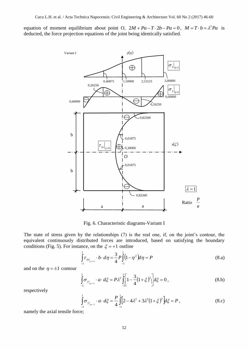
Fig. 6. Characteristic diagrams-Variant I

The state of stress given by the relationships (7) is the real one, if, on the joint’s contour, the

equivalent continuously distributed forces are introduced, based on satisfying the boundary

conditions (Fig. 5). For instance, on the 1 outline

1

1

1

1

214

3

1

PdPdbxy

(8.a)

and on the 1 contour

1

1

1

1

22 014

31

1

dPday , (8.b)

respectively

1

1

1

1

222 134241

PdP

day

, (8.c)

namely the axial tensile force;

Variant I

1 x

3,00000

2,53125

1,50000

0,46875

1 y

0,60000

0,60000

0,26250

0,26250

0 xy

0,82500

0,82500

0,01875

0,01875

0,30000

O

x

y

1

a

P Ratio

b

b

a

a


53

1

1

1

1

2222 134241

MPadPa

daay

, (8.d)

1

1

1

1

323

41141

TPdP

dayx

, (8.e)

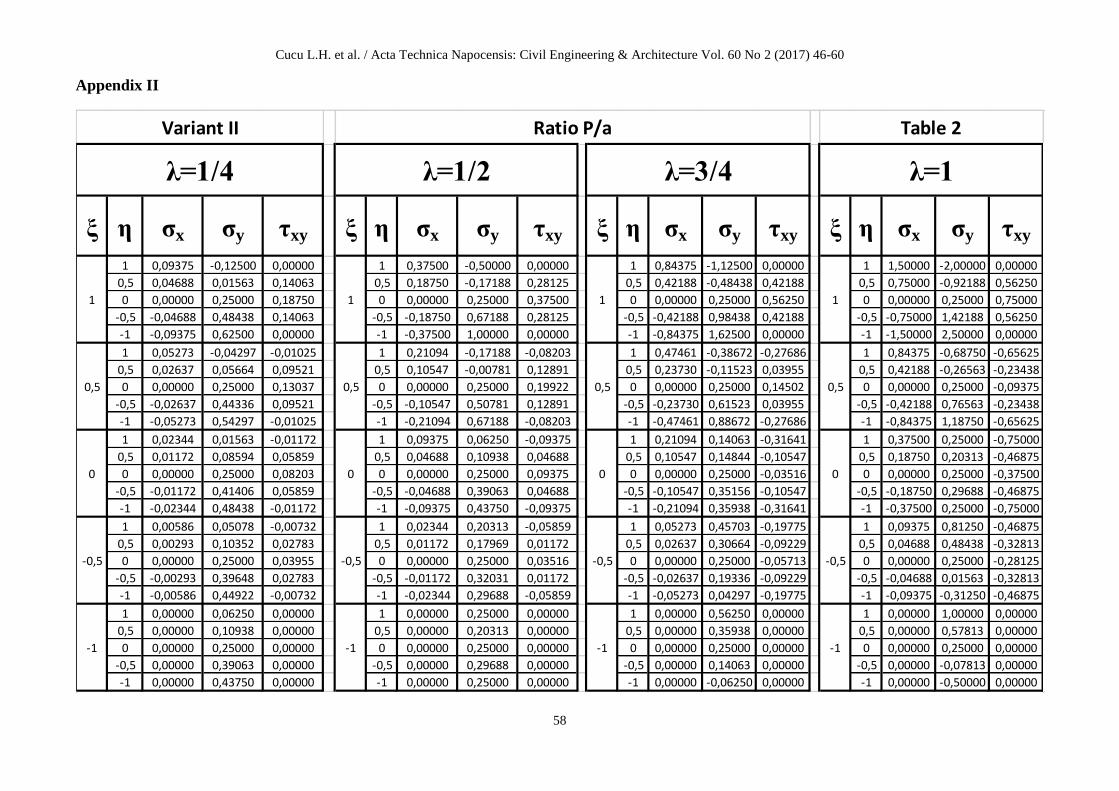
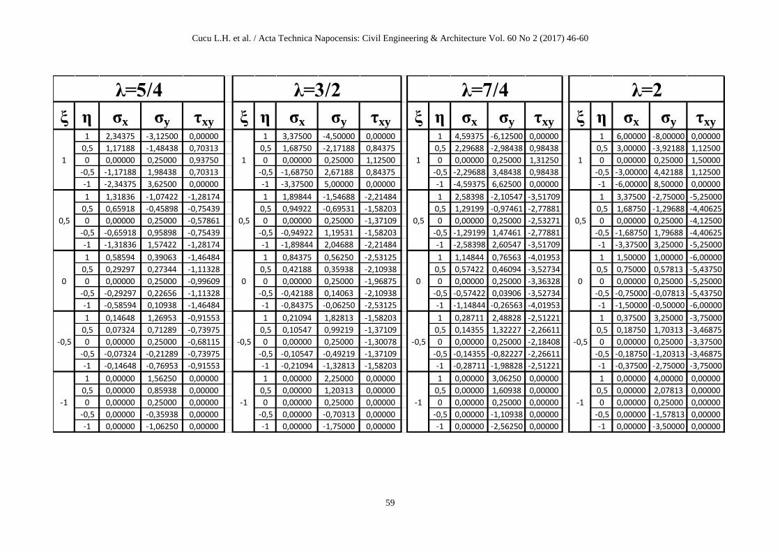
hence, the shear force. Several characteristic diagrams for the two variants, are shown in Fig. 6 and

7 and further details are given in Appendix I and II respectively.

Fig. 7. Characteristic diagrams-Variant II

4. Conclusions

In this way, the polynomial expressions of the biharmonic function yxF , 04 F given in [2]

and [5] are corrected, also the correct loading of the joint in the second variant is introduced; the

states of stress are properly determined in Tables 1 and 2 depicted in the Appendix I and II

respectively.

1

Factor

a

P

Variant II

1 x

1,50000

0,84375

0,37500

0,09375

0 xy

0,75000

0,75000

0,46875

0,46875

0,37500

0 xy

0,75000

0,09375

0,37500

0,28125

1 y

2,00000

2,50000

0,92188

1,42188

0,25000

y

x O

b

b

a

a


54

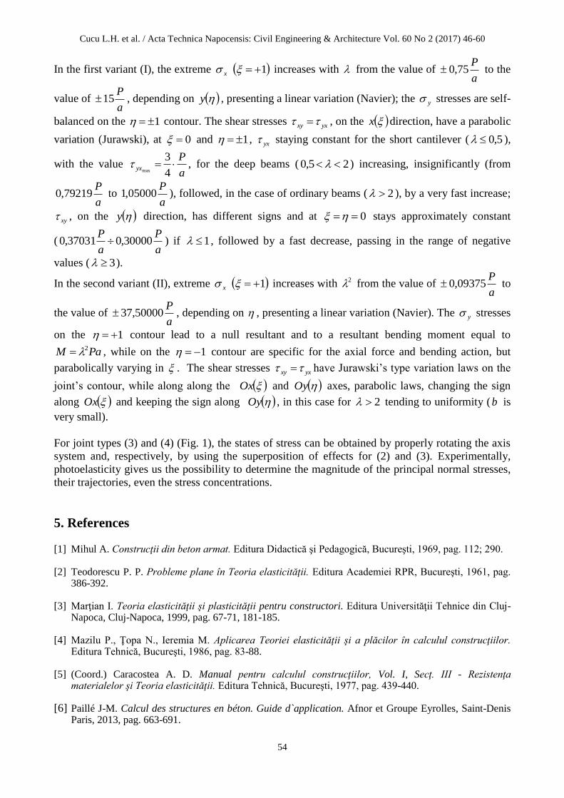
In the first variant (I), the extreme x 1 increases with from the value of a

P75,0 to the

value of a

P15 , depending on y , presenting a linear variation (Navier); the y stresses are self-

balanced on the 1 contour. The shear stresses yxxy , on the x direction, have a parabolic

variation (Jurawski), at 0 and 1 , yx staying constant for the short cantilever ( 5,0 ),

with the value a

Pyx

4

3max

, for the deep beams ( 25,0 ) increasing, insignificantly (from

a

P79219,0 to

a

P05000,1 ), followed, in the case of ordinary beams ( 2 ), by a very fast increase;

xy , on the y direction, has different signs and at 0 stays approximately constant

(a

P

a

P30000,037031,0 ) if 1 , followed by a fast decrease, passing in the range of negative

values ( 3 ).

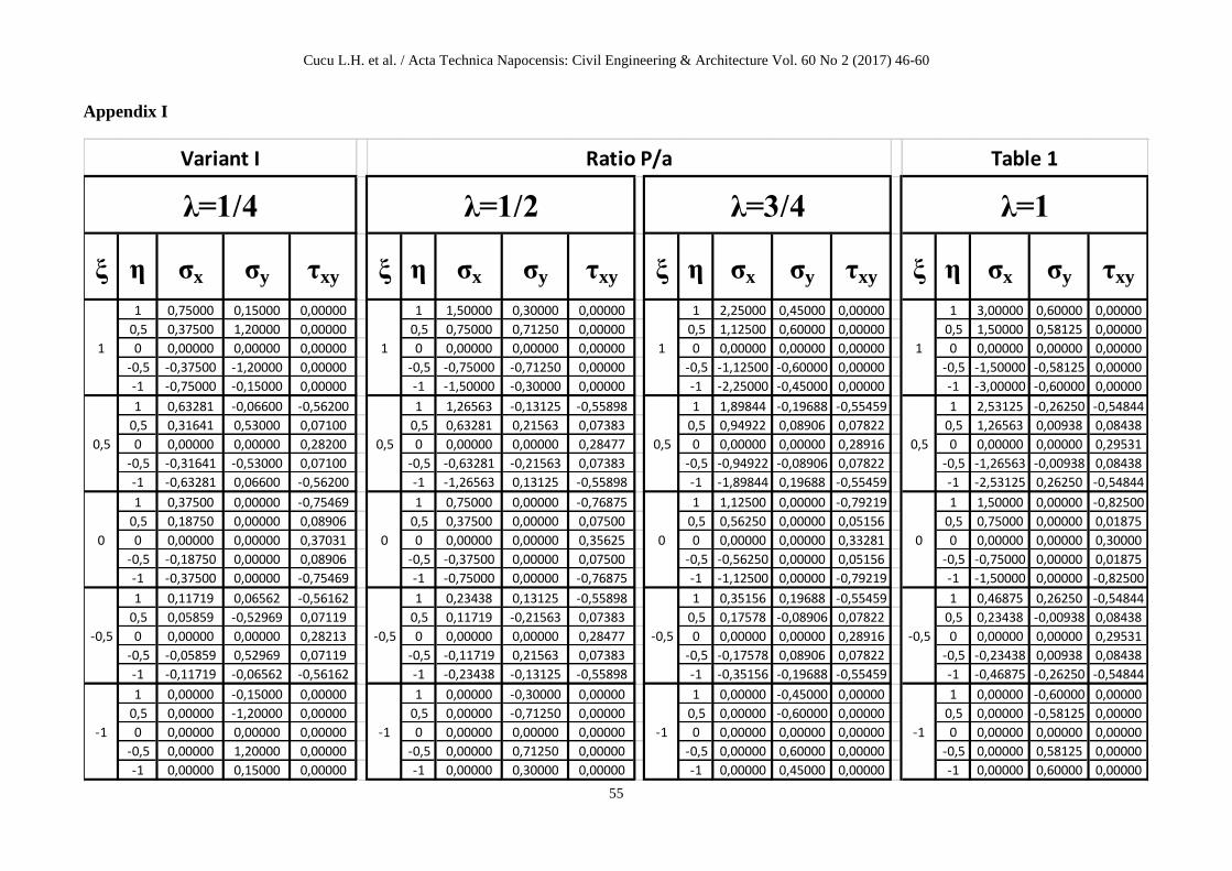
In the second variant (II), extreme x 1 increases with 2 from the value of a

P09375,0 to

the value of a

P50000,37 , depending on , presenting a linear variation (Navier). The y stresses

on the 1 contour lead to a null resultant and to a resultant bending moment equal to

PaM 2 , while on the 1 contour are specific for the axial force and bending action, but

parabolically varying in . The shear stresses yxxy have Jurawski’s type variation laws on the

joint’s contour, while along along the Ox and Oy axes, parabolic laws, changing the sign

along Ox and keeping the sign along Oy , in this case for 2 tending to uniformity (b is

very small).

For joint types (3) and (4) (Fig. 1), the states of stress can be obtained by properly rotating the axis

system and, respectively, by using the superposition of effects for (2) and (3). Experimentally,

photoelasticity gives us the possibility to determine the magnitude of the principal normal stresses,

their trajectories, even the stress concentrations.

5. References [1] Mihul A. Construcţii din beton armat. Editura Didactică şi Pedagogică, Bucureşti, 1969, pag. 112; 290.

[2] Teodorescu P. P. Probleme plane în Teoria elasticităţii. Editura Academiei RPR, Bucureşti, 1961, pag.

386-392. [3] Marţian I. Teoria elasticităţii şi plasticităţii pentru constructori. Editura Universităţii Tehnice din Cluj-

Napoca, Cluj-Napoca, 1999, pag. 67-71, 181-185. [4] Mazilu P., Ţopa N., Ieremia M. Aplicarea Teoriei elasticităţii şi a plăcilor în calculul construcţiilor.

Editura Tehnică, Bucureşti, 1986, pag. 83-88.

[5] (Coord.) Caracostea A. D. Manual pentru calculul construcţiilor, Vol. I, Secţ. III - Rezistenţa materialelor şi Teoria elasticităţii. Editura Tehnică, Bucureşti, 1977, pag. 439-440.

[6] Paillé J-M. Calcul des structures en béton. Guide d`application. Afnor et Groupe Eyrolles, Saint-Denis

Paris, 2013, pag. 663-691.


55

Appendix I

ξ η σx σy τxy ξ η σx σy τxy ξ η σx σy τxy ξ η σx σy τxy

1 0,75000 0,15000 0,00000 1 1,50000 0,30000 0,00000 1 2,25000 0,45000 0,00000 1 3,00000 0,60000 0,00000

0,5 0,37500 1,20000 0,00000 0,5 0,75000 0,71250 0,00000 0,5 1,12500 0,60000 0,00000 0,5 1,50000 0,58125 0,00000

0 0,00000 0,00000 0,00000 0 0,00000 0,00000 0,00000 0 0,00000 0,00000 0,00000 0 0,00000 0,00000 0,00000

-0,5 -0,37500 -1,20000 0,00000 -0,5 -0,75000 -0,71250 0,00000 -0,5 -1,12500 -0,60000 0,00000 -0,5 -1,50000 -0,58125 0,00000

-1 -0,75000 -0,15000 0,00000 -1 -1,50000 -0,30000 0,00000 -1 -2,25000 -0,45000 0,00000 -1 -3,00000 -0,60000 0,00000

1 0,63281 -0,06600 -0,56200 1 1,26563 -0,13125 -0,55898 1 1,89844 -0,19688 -0,55459 1 2,53125 -0,26250 -0,54844

0,5 0,31641 0,53000 0,07100 0,5 0,63281 0,21563 0,07383 0,5 0,94922 0,08906 0,07822 0,5 1,26563 0,00938 0,08438

0 0,00000 0,00000 0,28200 0 0,00000 0,00000 0,28477 0 0,00000 0,00000 0,28916 0 0,00000 0,00000 0,29531

-0,5 -0,31641 -0,53000 0,07100 -0,5 -0,63281 -0,21563 0,07383 -0,5 -0,94922 -0,08906 0,07822 -0,5 -1,26563 -0,00938 0,08438

-1 -0,63281 0,06600 -0,56200 -1 -1,26563 0,13125 -0,55898 -1 -1,89844 0,19688 -0,55459 -1 -2,53125 0,26250 -0,54844

1 0,37500 0,00000 -0,75469 1 0,75000 0,00000 -0,76875 1 1,12500 0,00000 -0,79219 1 1,50000 0,00000 -0,82500

0,5 0,18750 0,00000 0,08906 0,5 0,37500 0,00000 0,07500 0,5 0,56250 0,00000 0,05156 0,5 0,75000 0,00000 0,01875

0 0,00000 0,00000 0,37031 0 0,00000 0,00000 0,35625 0 0,00000 0,00000 0,33281 0 0,00000 0,00000 0,30000

-0,5 -0,18750 0,00000 0,08906 -0,5 -0,37500 0,00000 0,07500 -0,5 -0,56250 0,00000 0,05156 -0,5 -0,75000 0,00000 0,01875

-1 -0,37500 0,00000 -0,75469 -1 -0,75000 0,00000 -0,76875 -1 -1,12500 0,00000 -0,79219 -1 -1,50000 0,00000 -0,82500

1 0,11719 0,06562 -0,56162 1 0,23438 0,13125 -0,55898 1 0,35156 0,19688 -0,55459 1 0,46875 0,26250 -0,54844

0,5 0,05859 -0,52969 0,07119 0,5 0,11719 -0,21563 0,07383 0,5 0,17578 -0,08906 0,07822 0,5 0,23438 -0,00938 0,08438

0 0,00000 0,00000 0,28213 0 0,00000 0,00000 0,28477 0 0,00000 0,00000 0,28916 0 0,00000 0,00000 0,29531

-0,5 -0,05859 0,52969 0,07119 -0,5 -0,11719 0,21563 0,07383 -0,5 -0,17578 0,08906 0,07822 -0,5 -0,23438 0,00938 0,08438

-1 -0,11719 -0,06562 -0,56162 -1 -0,23438 -0,13125 -0,55898 -1 -0,35156 -0,19688 -0,55459 -1 -0,46875 -0,26250 -0,54844

1 0,00000 -0,15000 0,00000 1 0,00000 -0,30000 0,00000 1 0,00000 -0,45000 0,00000 1 0,00000 -0,60000 0,00000

0,5 0,00000 -1,20000 0,00000 0,5 0,00000 -0,71250 0,00000 0,5 0,00000 -0,60000 0,00000 0,5 0,00000 -0,58125 0,00000

0 0,00000 0,00000 0,00000 0 0,00000 0,00000 0,00000 0 0,00000 0,00000 0,00000 0 0,00000 0,00000 0,00000

-0,5 0,00000 1,20000 0,00000 -0,5 0,00000 0,71250 0,00000 -0,5 0,00000 0,60000 0,00000 -0,5 0,00000 0,58125 0,00000

-1 0,00000 0,15000 0,00000 -1 0,00000 0,30000 0,00000 -1 0,00000 0,45000 0,00000 -1 0,00000 0,60000 0,00000

-0,5

-1

λ=1

1

0,5

0

-0,5

-1

0

λ=1/4 λ=1/2 λ=3/4

1

0,5

1

0,5

-0,5

-1

1

0,5

0

-0,5

-1

Variant I Ratio P/a Table 1

0


56


1 3,75000 0,75000 0,00000 1 4,50000 0,90000 0,00000 1 5,25000 1,05000 0,00000 1 6,00000 1,20000 0,00000

0,5 1,87500 0,60000 0,00000 0,5 2,25000 0,63750 0,00000 0,5 2,62500 0,68571 0,00000 0,5 3,00000 0,74063 0,00000

0 0,00000 0,00000 0,00000 0 0,00000 0,00000 0,00000 0 0,00000 0,00000 0,00000 0 0,00000 0,00000 0,00000

-0,5 -1,87500 -0,60000 0,00000 -0,5 -2,25000 -0,63750 0,00000 -0,5 -2,62500 -0,68571 0,00000 -0,5 -3,00000 -0,74063 0,00000

-1 -3,75000 -0,75000 0,00000 -1 -4,50000 -0,90000 0,00000 -1 -5,25000 -1,05000 0,00000 -1 -6,00000 -1,20000 0,00000

1 3,16406 -0,32813 -0,54053 1 3,79688 -0,39375 -0,53086 1 4,42969 -0,45937 -0,51943 1 5,06250 -0,52500 -0,50625

0,5 1,58203 -0,05156 0,09229 0,5 1,89844 -0,10313 0,10195 0,5 2,21484 -0,14933 0,11338 0,5 2,53125 -0,19219 0,12656

0 0,00000 0,00000 0,30322 0 0,00000 0,00000 0,31289 0 0,00000 0,00000 0,32432 0 0,00000 0,00000 0,33750

-0,5 -1,58203 0,05156 0,09229 -0,5 -1,89844 0,10313 0,10195 -0,5 -2,21484 0,14933 0,11338 -0,5 -2,53125 0,19219 0,12656

-1 -3,16406 0,32813 -0,54053 -1 -3,79688 0,39375 -0,53086 -1 -4,42969 0,45937 -0,51943 -1 -5,06250 0,52500 -0,50625

1 1,87500 0,00000 -0,86719 1 2,25000 0,00000 -0,91875 1 2,62500 0,00000 -0,97969 1 3,00000 0,00000 -1,05000

0,5 0,93750 0,00000 -0,02344 0,5 1,12500 0,00000 -0,07500 0,5 1,31250 0,00000 -0,13594 0,5 1,50000 0,00000 -0,20625

0 0,00000 0,00000 0,25781 0 0,00000 0,00000 0,20625 0 0,00000 0,00000 0,14531 0 0,00000 0,00000 0,07500

-0,5 -0,93750 0,00000 -0,02344 -0,5 -1,12500 0,00000 -0,07500 -0,5 -1,31250 0,00000 -0,13594 -0,5 -1,50000 0,00000 -0,20625

-1 -1,87500 0,00000 -0,86719 -1 -2,25000 0,00000 -0,91875 -1 -2,62500 0,00000 -0,97969 -1 -3,00000 0,00000 -1,05000

1 0,58594 0,32813 -0,54053 1 0,70313 0,39375 -0,53086 1 0,82031 0,45937 -0,51943 1 0,93750 0,52500 -0,50625

0,5 0,29297 0,05156 0,09229 0,5 0,35156 0,10313 0,10195 0,5 0,41016 0,14933 0,11338 0,5 0,46875 0,19219 0,12656

0 0,00000 0,00000 0,30322 0 0,00000 0,00000 0,31289 0 0,00000 0,00000 0,32432 0 0,00000 0,00000 0,33750

-0,5 -0,29297 -0,05156 0,09229 -0,5 -0,35156 -0,10313 0,10195 -0,5 -0,41016 -0,14933 0,11338 -0,5 -0,46875 -0,19219 0,12656

-1 -0,58594 -0,32813 -0,54053 -1 -0,70313 -0,39375 -0,53086 -1 -0,82031 -0,45937 -0,51943 -1 -0,93750 -0,52500 -0,50625

1 0,00000 -0,75000 0,00000 1 0,00000 -0,90000 0,00000 1 0,00000 -1,05000 0,00000 1 0,00000 -1,20000 0,00000

0,5 0,00000 -0,60000 0,00000 0,5 0,00000 -0,63750 0,00000 0,5 0,00000 -0,68571 0,00000 0,5 0,00000 -0,74063 0,00000

0 0,00000 0,00000 0,00000 0 0,00000 0,00000 0,00000 0 0,00000 0,00000 0,00000 0 0,00000 0,00000 0,00000

-0,5 0,00000 0,60000 0,00000 -0,5 0,00000 0,63750 0,00000 -0,5 0,00000 0,68571 0,00000 -0,5 0,00000 0,74063 0,00000

-1 0,00000 0,75000 0,00000 -1 0,00000 0,90000 0,00000 -1 0,00000 1,05000 0,00000 -1 0,00000 1,20000 0,00000

-1

λ=7/4

1

0,5

0

-0,5

-1

λ=2

1

0,5

0

-0,5

-1

λ=5/4

1

0,5

0

-0,5

-1

λ=3/2

1

0,5

0

-0,5


57

ξ η σx σy τxy ξ η σx σy τxy

1 9,00000 1,80000 0,00000 1 15,00000 3,00000 0,00000

0,5 4,50000 0,99375 0,00000 0,5 7,50000 1,55625 0,00000

0 0,00000 0,00000 0,00000 0 0,00000 0,00000 0,00000

-0,5 -4,50000 -0,99375 0,00000 -0,5 -7,50000 -1,55625 0,00000

-1 -9,00000 -1,80000 0,00000 -1 -15,00000 -3,00000 0,00000

1 7,59375 -0,78750 -0,43594 1 12,65625 -1,31250 -0,21094

0,5 0,00000 0,00000 0,40781 0,5 6,32813 -0,62812 0,42188

0 0,00000 0,00000 0,40781 0 0,00000 0,00000 0,63281

-0,5 -3,79688 0,34688 0,19687 -0,5 -6,32813 0,62812 0,42188

-1 -7,59375 0,78750 -0,43594 -1 -12,65625 1,31250 -0,21094

1 4,50000 0,00000 -1,42500 1 7,50000 0,00000 -2,62500

0,5 2,25000 0,00000 -0,58125 0,5 3,75000 0,00000 -1,78125

0 0,00000 0,00000 -0,30000 0 0,00000 0,00000 -1,50000

-0,5 -2,25000 0,00000 -0,58125 -0,5 -3,75000 0,00000 -1,78125

-1 -4,50000 0,00000 -1,42500 -1 -7,50000 0,00000 -2,62500

1 1,40625 0,78750 -0,43594 1 2,34375 1,31250 -0,21094

0,5 0,70313 0,34688 0,19687 0,5 1,17188 0,62812 0,42188

0 0,00000 0,00000 0,40781 0 0,00000 0,00000 0,63281

-0,5 -0,70313 -0,34688 0,19687 -0,5 -1,17188 -0,62812 0,42188

-1 -1,40625 -0,78750 -0,43594 -1 -2,34375 -1,31250 -0,21094

1 0,00000 -1,80000 0,00000 1 0,00000 -3,00000 0,00000

0,5 0,00000 -0,99375 0,00000 0,5 0,00000 -1,55625 0,00000

0 0,00000 0,00000 0,00000 0 0,00000 0,00000 0,00000

-0,5 0,00000 0,99375 0,00000 -0,5 0,00000 1,55625 0,00000

-1 0,00000 1,80000 0,00000 -1 0,00000 3,00000 0,00000

-1

λ=5

1

0,5

0

-0,5

-1

λ=3

1

0,5

0

-0,5

Variant I

1 x

3,00000

2,53125

1,50000

0,46875

1 y

0,60000

0,60000

0,26250

0,26250

0 xy

0,82500

0,82500

0,01875

0,01875

0,30000

O

x

y

1

a

P Ratio

b

b

a

a


58

Appendix II


1 0,09375 -0,12500 0,00000 1 0,37500 -0,50000 0,00000 1 0,84375 -1,12500 0,00000 1 1,50000 -2,00000 0,00000

0,5 0,04688 0,01563 0,14063 0,5 0,18750 -0,17188 0,28125 0,5 0,42188 -0,48438 0,42188 0,5 0,75000 -0,92188 0,56250

0 0,00000 0,25000 0,18750 0 0,00000 0,25000 0,37500 0 0,00000 0,25000 0,56250 0 0,00000 0,25000 0,75000

-0,5 -0,04688 0,48438 0,14063 -0,5 -0,18750 0,67188 0,28125 -0,5 -0,42188 0,98438 0,42188 -0,5 -0,75000 1,42188 0,56250

-1 -0,09375 0,62500 0,00000 -1 -0,37500 1,00000 0,00000 -1 -0,84375 1,62500 0,00000 -1 -1,50000 2,50000 0,00000

1 0,05273 -0,04297 -0,01025 1 0,21094 -0,17188 -0,08203 1 0,47461 -0,38672 -0,27686 1 0,84375 -0,68750 -0,65625

0,5 0,02637 0,05664 0,09521 0,5 0,10547 -0,00781 0,12891 0,5 0,23730 -0,11523 0,03955 0,5 0,42188 -0,26563 -0,23438

0 0,00000 0,25000 0,13037 0 0,00000 0,25000 0,19922 0 0,00000 0,25000 0,14502 0 0,00000 0,25000 -0,09375

-0,5 -0,02637 0,44336 0,09521 -0,5 -0,10547 0,50781 0,12891 -0,5 -0,23730 0,61523 0,03955 -0,5 -0,42188 0,76563 -0,23438

-1 -0,05273 0,54297 -0,01025 -1 -0,21094 0,67188 -0,08203 -1 -0,47461 0,88672 -0,27686 -1 -0,84375 1,18750 -0,65625

1 0,02344 0,01563 -0,01172 1 0,09375 0,06250 -0,09375 1 0,21094 0,14063 -0,31641 1 0,37500 0,25000 -0,75000

0,5 0,01172 0,08594 0,05859 0,5 0,04688 0,10938 0,04688 0,5 0,10547 0,14844 -0,10547 0,5 0,18750 0,20313 -0,46875

0 0,00000 0,25000 0,08203 0 0,00000 0,25000 0,09375 0 0,00000 0,25000 -0,03516 0 0,00000 0,25000 -0,37500

-0,5 -0,01172 0,41406 0,05859 -0,5 -0,04688 0,39063 0,04688 -0,5 -0,10547 0,35156 -0,10547 -0,5 -0,18750 0,29688 -0,46875

-1 -0,02344 0,48438 -0,01172 -1 -0,09375 0,43750 -0,09375 -1 -0,21094 0,35938 -0,31641 -1 -0,37500 0,25000 -0,75000

1 0,00586 0,05078 -0,00732 1 0,02344 0,20313 -0,05859 1 0,05273 0,45703 -0,19775 1 0,09375 0,81250 -0,46875

0,5 0,00293 0,10352 0,02783 0,5 0,01172 0,17969 0,01172 0,5 0,02637 0,30664 -0,09229 0,5 0,04688 0,48438 -0,32813

0 0,00000 0,25000 0,03955 0 0,00000 0,25000 0,03516 0 0,00000 0,25000 -0,05713 0 0,00000 0,25000 -0,28125

-0,5 -0,00293 0,39648 0,02783 -0,5 -0,01172 0,32031 0,01172 -0,5 -0,02637 0,19336 -0,09229 -0,5 -0,04688 0,01563 -0,32813

-1 -0,00586 0,44922 -0,00732 -1 -0,02344 0,29688 -0,05859 -1 -0,05273 0,04297 -0,19775 -1 -0,09375 -0,31250 -0,46875

1 0,00000 0,06250 0,00000 1 0,00000 0,25000 0,00000 1 0,00000 0,56250 0,00000 1 0,00000 1,00000 0,00000

0,5 0,00000 0,10938 0,00000 0,5 0,00000 0,20313 0,00000 0,5 0,00000 0,35938 0,00000 0,5 0,00000 0,57813 0,00000

0 0,00000 0,25000 0,00000 0 0,00000 0,25000 0,00000 0 0,00000 0,25000 0,00000 0 0,00000 0,25000 0,00000

-0,5 0,00000 0,39063 0,00000 -0,5 0,00000 0,29688 0,00000 -0,5 0,00000 0,14063 0,00000 -0,5 0,00000 -0,07813 0,00000

-1 0,00000 0,43750 0,00000 -1 0,00000 0,25000 0,00000 -1 0,00000 -0,06250 0,00000 -1 0,00000 -0,50000 0,00000

Variant II Ratio P/a Table 2

0

-0,5

-1

1

0,5

0

-0,5

-1

λ=1/4 λ=1/2 λ=3/4

1

0,5

1

0,5

-0,5

-1

λ=1

1

0,5

0

-0,5

-1

0


59


1 2,34375 -3,12500 0,00000 1 3,37500 -4,50000 0,00000 1 4,59375 -6,12500 0,00000 1 6,00000 -8,00000 0,00000

0,5 1,17188 -1,48438 0,70313 0,5 1,68750 -2,17188 0,84375 0,5 2,29688 -2,98438 0,98438 0,5 3,00000 -3,92188 1,12500

0 0,00000 0,25000 0,93750 0 0,00000 0,25000 1,12500 0 0,00000 0,25000 1,31250 0 0,00000 0,25000 1,50000

-0,5 -1,17188 1,98438 0,70313 -0,5 -1,68750 2,67188 0,84375 -0,5 -2,29688 3,48438 0,98438 -0,5 -3,00000 4,42188 1,12500

-1 -2,34375 3,62500 0,00000 -1 -3,37500 5,00000 0,00000 -1 -4,59375 6,62500 0,00000 -1 -6,00000 8,50000 0,00000

1 1,31836 -1,07422 -1,28174 1 1,89844 -1,54688 -2,21484 1 2,58398 -2,10547 -3,51709 1 3,37500 -2,75000 -5,25000

0,5 0,65918 -0,45898 -0,75439 0,5 0,94922 -0,69531 -1,58203 0,5 1,29199 -0,97461 -2,77881 0,5 1,68750 -1,29688 -4,40625

0 0,00000 0,25000 -0,57861 0 0,00000 0,25000 -1,37109 0 0,00000 0,25000 -2,53271 0 0,00000 0,25000 -4,12500

-0,5 -0,65918 0,95898 -0,75439 -0,5 -0,94922 1,19531 -1,58203 -0,5 -1,29199 1,47461 -2,77881 -0,5 -1,68750 1,79688 -4,40625

-1 -1,31836 1,57422 -1,28174 -1 -1,89844 2,04688 -2,21484 -1 -2,58398 2,60547 -3,51709 -1 -3,37500 3,25000 -5,25000

1 0,58594 0,39063 -1,46484 1 0,84375 0,56250 -2,53125 1 1,14844 0,76563 -4,01953 1 1,50000 1,00000 -6,00000

0,5 0,29297 0,27344 -1,11328 0,5 0,42188 0,35938 -2,10938 0,5 0,57422 0,46094 -3,52734 0,5 0,75000 0,57813 -5,43750

0 0,00000 0,25000 -0,99609 0 0,00000 0,25000 -1,96875 0 0,00000 0,25000 -3,36328 0 0,00000 0,25000 -5,25000

-0,5 -0,29297 0,22656 -1,11328 -0,5 -0,42188 0,14063 -2,10938 -0,5 -0,57422 0,03906 -3,52734 -0,5 -0,75000 -0,07813 -5,43750

-1 -0,58594 0,10938 -1,46484 -1 -0,84375 -0,06250 -2,53125 -1 -1,14844 -0,26563 -4,01953 -1 -1,50000 -0,50000 -6,00000

1 0,14648 1,26953 -0,91553 1 0,21094 1,82813 -1,58203 1 0,28711 2,48828 -2,51221 1 0,37500 3,25000 -3,75000

0,5 0,07324 0,71289 -0,73975 0,5 0,10547 0,99219 -1,37109 0,5 0,14355 1,32227 -2,26611 0,5 0,18750 1,70313 -3,46875

0 0,00000 0,25000 -0,68115 0 0,00000 0,25000 -1,30078 0 0,00000 0,25000 -2,18408 0 0,00000 0,25000 -3,37500

-0,5 -0,07324 -0,21289 -0,73975 -0,5 -0,10547 -0,49219 -1,37109 -0,5 -0,14355 -0,82227 -2,26611 -0,5 -0,18750 -1,20313 -3,46875

-1 -0,14648 -0,76953 -0,91553 -1 -0,21094 -1,32813 -1,58203 -1 -0,28711 -1,98828 -2,51221 -1 -0,37500 -2,75000 -3,75000

1 0,00000 1,56250 0,00000 1 0,00000 2,25000 0,00000 1 0,00000 3,06250 0,00000 1 0,00000 4,00000 0,00000

0,5 0,00000 0,85938 0,00000 0,5 0,00000 1,20313 0,00000 0,5 0,00000 1,60938 0,00000 0,5 0,00000 2,07813 0,00000

0 0,00000 0,25000 0,00000 0 0,00000 0,25000 0,00000 0 0,00000 0,25000 0,00000 0 0,00000 0,25000 0,00000

-0,5 0,00000 -0,35938 0,00000 -0,5 0,00000 -0,70313 0,00000 -0,5 0,00000 -1,10938 0,00000 -0,5 0,00000 -1,57813 0,00000

-1 0,00000 -1,06250 0,00000 -1 0,00000 -1,75000 0,00000 -1 0,00000 -2,56250 0,00000 -1 0,00000 -3,50000 0,00000

-1

λ=7/4

1

0,5

0

-0,5

-1

λ=2

1

0,5

0

-0,5

-1

λ=5/4

1

0,5

0

-0,5

-1

λ=3/2

1

0,5

0

-0,5


60

ξ η σx σy τxy ξ η σx σy τxy

1 13,50000 -18,00000 0,00000 1 37,50000 -50,00000 0,00000

0,5 6,75000 -8,92188 1,68750 0,5 18,75000 -24,92188 2,81250

0 0,00000 0,25000 2,25000 0 0,00000 0,25000 3,75000

-0,5 -6,75000 9,42188 1,68750 -0,5 -18,75000 25,42188 2,81250

-1 -13,50000 18,50000 0,00000 -1 -37,50000 50,50000 0,00000

1 7,59375 -6,18750 -17,71875 1 21,09375 -17,18750 -82,03125

0,5 3,79688 -3,01563 -16,45313 0,5 10,54688 -8,51563 -79,92188

0 0,00000 0,25000 -16,03125 0 0,00000 0,25000 -79,21875

-0,5 -3,79688 3,51563 -16,45313 -0,5 -10,54688 9,01563 -79,92188

-1 -7,59375 6,68750 -17,71875 -1 -21,09375 17,68750 -82,03125

1 3,37500 2,25000 -20,25000 1 9,37500 6,25000 -93,75000

0,5 1,68750 1,20313 -19,40625 0,5 4,68750 3,20313 -92,34375

0 0,00000 0,25000 -19,12500 0 0,00000 0,25000 -91,87500

-0,5 -1,68750 -0,70313 -19,40625 -0,5 -4,68750 -2,70313 -92,34375

-1 -3,37500 -1,75000 -20,25000 -1 -9,37500 -5,75000 -93,75000

1 0,84375 7,31250 -12,65625 1 2,34375 20,31250 -58,59375

0,5 0,42188 3,73438 -12,23438 0,5 1,17188 10,23438 -57,89063

0 0,00000 0,25000 -12,09375 0 0,00000 0,25000 -57,65625

-0,5 -0,42188 -3,23438 -12,23438 -0,5 -1,17188 -9,73438 -57,89063

-1 -0,84375 -6,81250 -12,65625 -1 -2,34375 -19,81250 -58,59375

1 0,00000 9,00000 0,00000 1 0,00000 25,00000 0,00000

0,5 0,00000 4,57813 0,00000 0,5 0,00000 12,57813 0,00000

0 0,00000 0,25000 0,00000 0 0,00000 0,25000 0,00000

-0,5 0,00000 -4,07813 0,00000 -0,5 0,00000 -12,07813 0,00000

-1 0,00000 -8,50000 0,00000 -1 0,00000 -24,50000 0,00000

-1

λ=5

1

0,5

0

-0,5

-1

λ=3

1

0,5

0

-0,5

1

Ratio

a

P

Variant II

1 x

1,50000

0,84375

0,37500

0,09375

0 xy

0,75000

0,75000

0,46875

0,46875

0,37500

0 xy

0,75000

0,09375

0,37500

0,28125

1 y

2,00000

2,50000

0,92188

1,42188

0,25000

y

x O

b

b

a

a

a few data on the calculation of beam-column joints … · 2018-01-19 · and column and joints as...

Documents