School of Innovation, Design and Engineering Mälardalen International Master Academy (MIMA)

Master Program in Product and Process Development – Production and Logistics Management KPP231- Master Thesis Work, Innovative Production (Advanced Level 30 hp)

Advisor: Sariya Sripipat

Supervisor: Sabah Audo

A Feasibility Study of Setting-Up New Production Line – Either Partly Outsource a Process or Fully

Produce In-House.

Authors: Piansiri Cheepweasarash (740621-P180)

Sarinthorn Pakapongpan (780827-P188)

Abstract

This paper presents the feasibility study of setting up the new potting tray production line based on the two alternatives: partly outsource a process in the production line or wholly make all processes in-house. Both the qualitative and quantitative approaches have been exploited to analyze and compare between the make or buy decision. Also the nature of business, particularly SMEs, in Thailand has been presented, in which it has certain characteristics that influence the business doing and decision, especially to the supply chain management. The literature relating to the forecasting techniques, outsourcing decision framework, inventory management, and investment analysis have been reviewed and applied with the empirical findings. As this production line has not yet been in place, monthly sales volumes are forecasted within the five years time frame. Based on the forecasted sales volume, simulations are implemented to distribute the probability and project a certain demand required for each month. The projected demand is used as a baseline to determine required safety stock of materials, inventory cost, time between production runs and resources utilization for each option. Finally, in the quantitative analysis, the five years forecasted sales volume is used as a framework and several decision making-techniques such as break-even analysis, cash flow and decision trees are employed to come up with the results in financial aspects Keywords: Outsourcing, decision making, inventory cost, SMEs, resource utilization, break-even, cash flow, decision tree.

I

Acknowledgement We would like to take this opportunity to thank many people who being so supportive and very much encouraging us in making this thesis possible. To our supervisor, Sabah Audo, who always gives us the prompt advices and responses on our questions as well as the guidance on the project’s direction. To K.T Plastics Agriculture Limited., Partnership, for giving us the opportunity to work on this project ,and thus allowing us to apply the literature knowledge to the real situations and practices. A special thanks is given to Ms Sariya Sripipat, who dedicated her precious time in coordinating and kindly provided all the necessary information, which ease us in doing this project from different location feasible. To our brothers, sisters, friends, and especially our parents, who always besides us, give valuable advise, and help us get through the difficult times, thanks for all the emotional support and caring.

II

Table of Contents ABSTRACT ............................................................................................................................................ I ACKNOWLEDGEMENT ....................................................................................................................II TABLE OF CONTENTS .................................................................................................................... III CHAPTER 1: INTRODUCTION .........................................................................................................1

1.1 BACKGROUND ................................................................................................................................1 1.2 PROBLEM IDENTIFICATION .............................................................................................................2 1.3 PURPOSE OF STUDY ........................................................................................................................2 1.4 PRODUCT DESCRIPTION ..................................................................................................................2 1.5 PRODUCTION PROCESS ...................................................................................................................3

1.5.1 Process Mapping: Potting Trays ...........................................................................................4 1.6 PROJECT DIRECTIVES......................................................................................................................5 1.7 PROJECT LIMITATIONS....................................................................................................................5

CHAPTER 2: THEORETICAL BACKGROUND .............................................................................6 2.1 FORECASTING TECHNIQUES............................................................................................................6

2.1.1 Qualitative Methods...............................................................................................................6 2.1.2 Quantitative Methods.............................................................................................................6 • Historical Projection or Time Series Methods ......................................................................6 • Causal Methods.....................................................................................................................7

2.2 OUTSOURCING ................................................................................................................................8 2.2.1 Definition of Outsourcing ......................................................................................................8 2.2.2 The reason for outsourcing decision......................................................................................9 2.2.3 Disadvantage of outsourcing ...............................................................................................12 2.2.4 Methods to avoid the problem of outsourcing......................................................................14 2.2.5 Outsourcing decision framework .........................................................................................14 • A composite outsourcing decision .......................................................................................14 • A conceptual Framework for evaluating the make or buy decision ....................................16

2.3 INVENTORY...................................................................................................................................20 2.3.1 Role of Inventory..................................................................................................................20 2.3.2 Type of Inventory .................................................................................................................21 2.3.3 Inventory Cost......................................................................................................................23 • Non-instantaneous Replenishment ......................................................................................25 2.3.4 Inventory Control System.....................................................................................................26 • Independent Demand...........................................................................................................27 • Dependent Demand .............................................................................................................28

2.4 FEASIBILITY STUDY AND INVESTMENT ANALYSIS........................................................................30 2.4.1 Feasibility Study...................................................................................................................30 2.4.2 Investment Analysis..............................................................................................................30 • Cash on cash return ............................................................................................................30 • Payback Period ...................................................................................................................31 • Internal Rate of Return........................................................................................................31 • Net Present Value................................................................................................................31

CHAPTER 3: EMPIRICAL STUDY..................................................................................................32 3.1 SALES FORECAST..........................................................................................................................32

3.1.1 Annual Sales Forecast: Linear Regression..........................................................................33 3.1.2 Monthly Sales Forecast: Seasonal Patterns.........................................................................34 3.1.3 Forecast Accuracy ...............................................................................................................38

3.2 AN OVERVIEW OF BUSINESS IN THAILAND: SMALL AND MEDIUM ENTERPRISE (SMES)..............40 3.2.1 SMEs Definition by Thai Government .................................................................................40

3.3 PREVIOUS OUTSOURCING..............................................................................................................43

III

3.3.1 Stage one: Define the core activities of the business ...........................................................46 3.3.2 Stage two: Profile the appropriate value chain links...........................................................49 3.3.3 Stage three: Total cost analysis of core activities................................................................51 3.3.4 Stage four: Analysis of potential suppliers for partnership .................................................52

3.4 INVENTORY APPLICATION ............................................................................................................53 3.4.1 Sales Forecast and Demand Simulation ..............................................................................53 3.4.2 Inventory Cost......................................................................................................................59 • Inventory Carrying cost.......................................................................................................59 • Setting-Up Cost ...................................................................................................................60 3.4.3 Ordering Quantity (Lot-Sizing)............................................................................................61 3.4.4 Time between Production Runs (TBP) and Resources Utilization.......................................68

CHAPTER 4: ANALYSIS AND RESULT.........................................................................................73 4.1 QUANTITATIVE ANALYSIS: DECISION-MAKING TECHNIQUES ......................................................73

4.1.1 Break-Even Analysis: Make or Buy .....................................................................................73 4.1.2 Cash Flow Analysis..............................................................................................................76 4.1.3 Decision Tree Analysis.........................................................................................................79

4.2 AGGREGATE ANALYSIS AND RESULT ...........................................................................................84 CHAPTER 5: CONCLUSIONS AND RECOMMENDATIONS.....................................................85 REFERENCES .....................................................................................................................................87 APPENDIX ...........................................................................................................................................92

IV

Chapter 1: Introduction

1.1 Background Established since May 2000, KT Plastic Agriculture Limited Partnership is a family own business located in Bangkok, Thailand. With the registered capital of THB 5 million, the company has an approximated turnover of THB 36 million in 2007. KT Plastic Agriculture Ltd. Part. is a manufacturer and a distributor of plastic products using in agricultural field. Since the aim of the company is to be a one-stop supply point for customers in agricultural industry, it strives to broaden product lines at less cost. Currently, the company have owned manufacturing on the products that fit their core competency, outsources the production of some products to other plastic manufacturers in related industry who can do it in a cost effective way, and become the distributor of some other products such as shade net, mesh netting, nylon net and peat moss that require a huge production scale in which the company has insufficient capability to produce them at this moment. Currently, there is one type of machine, extruder blowing machine, used in the company to produce various products, for example plastic mulching film, plastic bags for agricultural purpose, garbage bags, plastics for green house, etc. For products like plastic potting trays that need to be produced by vacuum forming machine, they are currently outsourced. The company’s main production line is mulching film. During these years, potting tray is another product which sells along side with mulching film but the company previously does not produce potting trays in-house, due to the lack of technical skills and knowledge in production. The company was previously a trader and later becomes a manufacturer. Thus, in the beginning, the company chose mulching film as their core product and invested on this production line while outsourced potting tray. Manufacturing potting-tray in-house has been in consideration for the company since the company started expanding to manufacturing business. Yet, at that time, with the limited knowledge in technology, technical skills and expertise in manufacturing market, the company has not yet decided to perform the production of the potting tray in-house. Also, at the previous location, the company had lack of space for establishing potting tray production line, but this problem had been eliminated since the company moved to the new factory location on 2006. Another reason that holds the company back from proceeding the in-sourcing of this product line is because the company can still sell potting tray with profit through outsourcing. However, during these years, because the sales of potting tray has increased and a certain market shares are owned by the company, the sales volume of potting trays proves to be relatively high compared to other product lines except mulching films which is still considered as a core product for the company. Thus, the company would like to investigate the feasibility of having their own production for potting trays. Moreover, recently, the company faces problems from outsourcing of potting tray due to the supplies’ quality, and the threat from suppliers that they become the company’s competitors. The problem has arisen when the company hires other manufacturers to

1

produce, not only the company has to pay for the creation of new mold but also the suppliers would have the mold for that product. Though these plastic manufacturers whom the company outsource is closed to the company’s business market, yet they in different industry, they can produce the products using the company’s mold and supply it to other customers, becoming the company’s direct competitors. This issue triggers the company to reconsider soberly in acquiring back the production of potting trays in-house.

1.2 Problem Identification Current situation of outsourcing the whole potting tray production line gives some threats to KT Plastics rather than opportunities. Deciding to backsource the whole production line, with limited resources, the company needs to thoroughly identify the core process of this production line and make sure to keep this process to be performed in-house. However, for the other non-core processes, the company also needs to evaluate the option of outsourcing and in-house making to see which one would offer the best opportunity. The two options the company is considering are as followed:

• Option 1: Company would invest in the thermoforming machine while buying plastic sheets from supplier (partly outsource).

• Option 2: Company would manufacture everything in-house by investing in

the sheet extrusion machine and thermoforming machine.

1.3 Purpose of Study The aim of this study is to help KT Plastics to achieve an effective decision making with regard to the setting up of new potting tray production line, providing both qualitative and quantitative aspects to consider. Since the company decides to invest in this vacuum forming machine (core process), they want to make the most out of their investment. Therefore, the company wants us to perform the feasibility study of establishing the new production line of potting tray, evaluating whether manufacturing all production processes in-house or partly outsourcing a process would be more efficient and yield a better profit.

1.4 Product Description The plastic potting tray is made by the plastic type PS (polystyrene). The potting tray is used in the agriculture field to grow seeds before planting into the land field. With the dimension of 55cm x 36cm x 70 micron and weight 160 gram, a tray can have different number of holes, yet the potting tray with 72 holes and 104 holes is widely used and highly demanded in the market.

2

1.5 Production Process The production line of potting tray consists of two sub-production processes, in which each process will be contained in a production cell that can be separated from each other. There are two main machines used in the potting tray production line; one is the sheet extrusion machine and the other is thermoforming machine.

Sheet extrusion machine

Thermoforming machine

3

1.5.1 Process Mapping: Potting Trays

Packing

Trimming & Punching

Machine

Sheet Extrusion Machine

Stock some in inventory

Thermoforming Machine

Mixing Machine

Plastic PS

Black Color

4

As illustrated in the process mapping, the production of potting tray starts with mixing Polystyrene (PS) plastic with mater batches: black color in the mixing machine. This process will take approximately 15 minutes. When the mixture is ready, mixed plastics will be taken out and put into sheet extrusion machine. Then, the extrusion machine will process plastics into a roll of plastic sheet. In this step, it can process 140kg of plastics per an hour, depending on the capacity of machine. After that, a roll of plastic sheet will be taken to a station of thermoforming machine and some of the plastic sheet rolls will be kept in the inventory, waiting to be processed further in the thermoforming machine. At the thermoforming station, a staff will feed plastic sheet into thermoforming machine, processing to be potting tray with the cycle time of approximately 75 seconds per two trays. Then, this potting tray will pass through the process of edges trimming and holes punching, finally, to the packing process with 100 trays per box and ready to be delivered. Among the production processes of this product line, thermoforming machine is considered as the company’s core competency since forming plastic sheet into shape requires molds. The variation of the product in this production line depends on molds, for example 104 holes potting tray and 72 holes potting tray requires different set of molds whereas these products use the same type of plastic sheet to feed into thermoforming machine.

1.6 Project Directives As KT Plastics has to decide between the two options of partly outsource or wholly-produce in-house the potting tray production line, the company has given certain conditions and requirements to use as a scope for this study. Expecting to have a return on investment within five years and the total production cost of product should not exceed the current price of buying from supplier or at least the company should be able to sell to its customers at the same selling price and is still profitable, thus, this study of feasibility is set the timeframe to be within five years. Given a few years historical sales data, five years sales forecast of potting tray is developed to use as framework to compare and evaluate between the two options.

1.7 Project Limitations Our study present the solution based on the maximum production time available, three working shifts, and the optimism of market trend. Since the production line has not yet been in place, there might be unforeseen circumstances emerging such as unplanned stop-time, machine break-down, market fluctuation, changes in government policy, level of competition, etc., when the actual production line has been setup, thus deviate the result from what has been analyzed and presented. Due to different time zone and location between the company and the authors, there is a difficulty in gathering some data and information from both the suppliers and the company.

5

Chapter 2: Theoretical Background

2.1 Forecasting Techniques Forecasting demand levels is essential to the firm as a whole as it provides the basic inputs for the planning and controlling the use of limited resources in all functional areas (Ballou, 2004). The objective of forecasting is to develop a useful forecast by applying information at hand with the forecasting technique that best fit the different pattern of demand, such as spatial/ temporal demand, lumpy/ regular demand, and derived/ independent demand. Forecasting methods are categorized into two types: qualitative and quantitative methods.

2.1.1 Qualitative Methods Qualitative or judgment methods are those that use intuition e.g. management or expert opinions, surveys, or comparative techniques to produce quantitative estimates about the future. The available information relating to the forecasting factors are nonquantitative and subjective (Ballou, 2004). Judgment method is useful when there is inadequate historical data. Due to the nature of the nonscientific methods, it makes them difficult to standardize and validate for accuracy. However, in some cases like predicting the success of new products, government policy changes, or the impact of new technology, judgment methods are the only practical way to make a forecast. It can be used to modify the forecast that generated by quantitative methods to anticipate the special events so as to reflect and give a more reliable forecasts and to adjust the historical data that will be analyzed with the quantitative method in order to minimize the impact of special events that occurred in the past. Qualitative or judgment methods are likely to be the choice for all time horizons of forecasting: short term, medium term and long term.

2.1.2 Quantitative Methods Quantitative methods include historical projection methods or time series models and causal methods. They rely heavily on historical information to predict or project the future demand.

• Historical Projection or Time Series Methods When an adequate amount of historical data is available and the trend and seasonal patterns in the time series are stable and well defined, projecting these data into the future can be an effective way of forecasting for the short-term.

6

Identifying the underlying patterns of demand that combine, time series analysis produces an observed historical pattern and then develops a model to replicate the past pattern (Krajewski, Ritzmand, Malhotra, 2007). The quantitative nature of the time series encourages the use of mathematical or statistical approach as the primary forecasting tools. Different time series method such as naïve forecast, simple moving averages, weighted moving averages, exponential smoothing, trend, and seasonal forecast are used to address various patterns of demand. The time series models are reactive in nature. They track change by being updated as new data become available, a feature that allows them to adapt to changes in trend and seasonal pattern. Yet, if the change is rapid, the models do not signal the change until after it has occurred (Ballou, 2004). Nevertheless, this limitation is not serious when forecasts are made over short time horizons unless changes are particularly dramatic.

• Causal Methods Causal methods are used when historical data are available. The fundamental ground on which causal methods are built is that when the relationship between the factor to be forecasted (e.g. sales volume) and other external or internal factors (e.g. government actions or advertising campaign) can be identified as the cause-and-effect relationship. These relationships are expressed in a variety of forms (statistical, e.g. regression and econometric models; and descriptive, e.g. input-output, life cycle, and computer simulation models) and can be complex. Each model is derived its validity from the historical patterns that establish the association between the predicting variables and the variable to be forecasted (Ballou, 2004). Causal methods provide the most sophisticated forecasting tools and are good for predicting turning points in demand and for preparing long-term forecasts (Krajewski, Ritzmand, Malhotra, 2007).

7

2.2 Outsourcing

The management of an outsourced process is fundamental for the future growth of a firm (Fine and Whitney, 1996; Ruffo, Tuck and Hague, 2007). Outsourcing is the act of transferring the work to an external party. Whether or not to outsource is the decision of whether to make or to buy. Organizations continuously face with the decision of whether to expand with existing to create an asset, resource, product or service internally or to buy it from an external party (Power, Desouza and Bonifazi, 2006). Making the wrong decision for outsourcing can result in cost overruns, project delays, or solution that does not fit business needs.

2.2.1 Definition of Outsourcing Fill and Visser stated that Hiemstra and van Tilburg (1993) define outsourcing as: subcontracting the custom-made articles and constructions, such as components, sub-assemblies, final products, adaptations and/or services, to another company. According to Bendor-Samual (1998), outsourcing provides certain leverage that is not available to a company’s internal departments. This leverage may have many dimensions: economies of scale, process expertise, access to capital, access to expensive technology, etc. The combination of these dimensions creates the cost savings inherent in outsourcing. Mylott (1995) views outsourcing in terms of full outsourcing, selective outsourcing, and everything-in-between outsourcing. Full outsourcing refers to the vendors who are in charge for all activities while, in selective outsourcing, the vendor provides services for one or a few activities such as payroll. Everything-in-between outsourcing is exactly to the meaning of its name. Mornme (2001) indicates different sourcing strategies: make or buy, outsourcing, in-sourcing, and strategic sourcing. Doing everything in-house might be manageable, but it is not always efficient. Outsourcing is an effective tool, and when exploits reasonably it can become a key factor for change, irrespective of whether the change is radical or incremental (Rebernik and Bradac, 2006). Outsourcing implies a business relationship between two parties: the outsourcing subject (also called the principal or the client) who makes the decision of whether to outsource or not; and an external outsourcing firm (also called the supplier or subcontractor) (Arnold, 2000). Outsourcing occurs when a company uses an outside firm to provide a necessary business function that might otherwise be done in-house. It is a strategic management tool for transferring part of the business process to another company; its aim is predominantly to make a company more competitive by enabling it to stay focused on core competencies (Rebernik and

8

Bradac, 2006). Gillley and Rasheed (2000) also point out that outsourcing occurs in two situations. First is when the client outsources activities that were originally sourced internally, resulting from a vertical disintegration decisions. Secondly, when the client sources activities that are within the client’s capabilities, and hence could have been sourced internally, although they have not been completed in-house in the past The major distinction between outsourcing and subcontracting are when the outsourced activities are specific to the client. The outsourced activities must perform according to a plan, specification, form or design, varying detail, provided by the client (Webster et al., 1997). Hence, a firm buying an off-the-shelf, standardized component or a supplier’s proprietary part is not considered as outsourcing as no customization is performed for the buyer (Sousa and Voss, 2007).

2.2.2 The reason for outsourcing decision

Traditionally, buying by organizations had been done largely on the basis of obtaining the best price, exceptionally taking into account a few other factors such as quality and delivery (Mclvor and Humphreys, 2000). In general, there exist three main clusters of reasons driving the outsourcing decision – reducing cost, improving operational performance and developing competencies (Rebernik and Bradac, 2006). Beulen (1994) defined five drivers of outsourcing which are quality, cost, finance, core-business and cooperation (Fill and Visser, 2000). As well as, Winkleman et al. (1993) stated that there are two basic drivers behind the growth of outsourcing, cost reduction and a strategic shift in the way that organizations are managing their business. However, in many cases, the significant numbers of factors such as delivery reliability, technical capability, cost capability and the financial stability of suppliers were not taken into consideration (Dooley, 1995). Few organizations have taken a strategic view of make or buy decisions while many companies decide to buy rather than make for short-term reasons of cost reduction and capacity (Ford et al., 1993; Humphreys et al., 2000).

9

Table 1: Drivers for outsourcing by Beulen et al., 1994

Quality Actual capacity is temporarily insufficient to comply with demand. The quality motive can be subdivided into three aspects: increase quality demands, shortage of qualified personnel, and outsourcing as a transition period. Cost Outsourcing is a possible solution to control increasing costs and to combine it with a cost leadership strategy. By controlling and decreasing costs, a company can increase its competitive position. Finance A company has a limited investment budget. The funds must be used for investment in core business activities, which are long-term decisions. Core-business Core-business is a primary activity with which an organization generates revenues. A company should pay a strategic attention to the core-business activities, while all subsequent activities are mainly supportive and should be outsourced. Cooperation Cooperation between companies can lead to conflict. In order to avoid such conflict those activities that are produced by both organization should be subject to total outsourcing.

Source: Fill C. and Visser E. (2000), “The outsourcing dilemma: a composite approach to the make or buy decision”, Management Decision, Vol. 38 No. 1, pp. 43-50. Outsourcing can free up assets and reduce cost in the immediate financial period. Outsourcing parts of the in-house operations, organizations report significant savings on operational and capital costs (Harland et al., 2005). McCarthy and Anagnostou (2004) summarize the reasons for outsourcing, which are:

Exploit external supplier investments, innovations and capacities.

Reduce operating costs, whilst increasing focus on core competencies.

There are several other motivations for outsourcing beyond short-term cost savings. Outsourcing improves flexibility to meet changing business conditions, demand for products, services and technologies (Greaver, 1999). The Outsourcing Institute proposed the reasons when organizations choose outsourcing as an alternative rather than hiring full-time employee. From a Survey of Current and Potential Outsourcing End Users in 1998, there are ten most important reasons for organizations to outsource; (Ashe, 1999)

• Reduced operating costs: Companies trying to do everything themselves may incur very high deployment expenses, all of which are passed on to the customers. An outside provider's lower cost structure, which may be the result of a greater economy of scale or other advantage based on specialization, reduces a company's operating costs and increases its competitive advantage.

10

• Improved company focus: Outsourcing allows a company to focus on its core competencies by having operational functions assumed by an outside expert.

• Access to experts and specialists: Experts and specialists make extensive investments in technology, procedures, and people. Expertise can be gained by working with many clients who face similar obstacles. This combination of specialization and expertise gives customers a competitive advantage and helps them to avoid the cost of investment and training.

• Freeing of resources for other purposes: Every organization has the limitation on the resources availability. Outsourcing allows an organization to redirect its resources, most often people, from noncore activities toward strategic activities that serve its customers.

• Resources not available internally: Companies outsource because they do not have access to the required resources within the company. Outsourcing is a good alternative to build the needed capability from the beginning.

• Improved efficiency: To improve efficiency, a company must aim for dramatic improvements in critical measures of performance such as cost, quality, service, and speed. In some instances, the need to increase efficiency can directly conflict with the need to invest in the primary focus of the business. Outsourcing the non-core functions to a specialist allows the organization to realize the benefits of maximizing efficiency.

• Better control over difficult or complex functions: Outsourcing is a smart option for managing complex tasks. When a function is viewed as complex or out of control, the organization needs to examine the underlying causes. The organization must understand its own needs in order to communicate those needs to an outside provider.

• Reduced capital expenditures: There is an enormous competition within most organizations for capital funds. Deciding where to invest these funds is one of the most important decisions that top management makes. It is often difficult to justify secondary capital investments when primary departments compete for the same money. Outsourcing can reduce the need to invest capital funds in these secondary business functions.

• Reduced risk: Tremendous risks are associated with the investments an organization makes. All aspects of the environment—such as markets, competition, government regulations, financial conditions, and technologies—change rapidly.

• Asset infusion: Outsourcing often involves the transfer of assets from the customer to the provider. Equipment, facilities, vehicles, and licenses used in the internal operations have value and are sold to the supplier. Certain assets sold to the supplier reveal a win–win approach for both parties.

11

2.2.3 Disadvantage of outsourcing

Although there are many advantages to outsourcing, there are also a number of disadvantages. In some instances, advantages can become disadvantages, depending on the organization and the problems involved. Some organizations do not achieve the expected benefits from outsourcing, Lonsdale (1999) and Mclvor (2000) survey suggested that only 5 percent of companies achieved significant benefits from outsourcing. Fill and Visser (2000) also added that companies that continue to make sourcing decisions based solely on cost will eventually wither and die.

There is an initial tendency to overstate benefits and that the suppliers are likely to perform better in the beginning of the contract to make first good impressions (Schwyn, 1999). Lonsdale (1999) highlighted reasons for this: focusing from achieving short-term benefits; lacking of formal outsource decision-making processes, as well as medium and long-term cost benefit analyzed complexity in the total supply network. Anderson and Anderson (2000) identified three main problem that might occurs which are;

1. The diffusion of secret information. 2. The direct dependence on suppliers; they can cause delays or

other problems 3. Losing the knowledge to integrate what has been outsourced,

expanding in the long-term, costs of integration. As quoted by Ashe (1999) in “Outsourcing relationships: why are they difficult to manage?” the research by InfoServer (1999) stated that the drawbacks of outsourcing include the following:

• No benefit from a drop in cost of work outsourced: In some industries, when a long-term contractual agreement ends, a drop in the cost of outsourcing work does not necessarily mean a lowering of the cost to perform the work internally.

• Problems occurring in the aftermath of layoffs/downsizing: Morale becomes a concern in the aftermath of some outsourcing deals. The remaining employees might have to work more extensively, struggling with problems such as meeting schedules, budget, and quality specifications while getting the same rate of pay.

• Outsourcing impeding the work of the organization: On rare occasions, organizations have experienced production delays caused by the outsourcing provider

• Managing long-term relationships: Several factors contribute to a not-so-perfect outsourcing relationship. The factors include (1) pricing and service levels, (2) differing buyer and supplier cultures, (3) lack of flexibility in long-term contracts leading to increased dissatisfaction, (4) both parties failing to make the most of the relationship at the expense of one another, (5) underestimating the time and attention required to manage the relationship or giving management responsibility to the vendor, and (6) lack of management oversight.

12

In addition to benefits and risks, Kremic, Tukel and Rom (2006) had analyzed outsourcing literatures and listed factors which may impact outsourcing decisions, showing on the Table 2 below; Table 2: Expected benefits and Potential risks of outsourcing

Expected benefits Potential risks Cost saving Reduce capital expenditures Capital infusion Transfer fixed costs to variable Quality improvement Increase speed Greater flexibility Access to latest technology/infrastructure Access to skills and talent Augment staff Increase focus on core functions Get rid of problem functions Copy competitors Reduced politic pressures or scrutiny Legal compliance Better accountability/management

Unrealized savings or hidden costs Less flexibility Poor contract or poor selection of partner Loss of knowledge/skills and/or

cooperate memory and the difficulty in reacquiring a function

Loss of control/core competencies Power shift to supplier Supplier problems (poor performance or

bad relations, opportunistic behavior, not giving access to best talent or technology

Lost customers, opportunities, or reputation

Uncertainty/changing environment Poor morale/employee issues

Other: Loss of synergy Create competitor Conflict of interest Security issues False sense of irresponsibility Legal obstacles Skill erosion

Source: Kremic, T., Tukel, O.I. and Rom, W.O. (2006), “Outsourcing decision support: a survey of benefits, risks, and decisions factors”, Supply Chain Management: An International Journal, Vol. 11 No. 6, pp. 467-482. Harland et al. (2006) reviewed outsourcing literatures and assessed the risks and benefits on outsourcing, adding more benefits/opportunities in organizations unit such as increasing ability to meet changing market needs, providing benefit through economies of scale and scope, freeing constraints of in-house cultures and attitudes, and providing fresh ideas and objective creativity. However, it also notes that the risks of failure to identify core and non-core activities can lead organizations to outsource their competitive advantage. Once an organizational competency is lost, it is difficult to rebuild. Combining strategic aspects with a rigorous cost analysis, organizations are in better positions that move them closer to their longer term goals (Fill and Visser, 2000).

13

2.2.4 Methods to avoid the problem of outsourcing

Ruffo, Tuck and Hague (2007) suggested methods to avoid these problems include:

Taking long-term view. Never outsource core capabilities. Prudently examine if any critical activities need to be outsourced, though

only partially. If outsourcing is made on a critical function, use two or more suppliers,

in order to maintain quality and price competition. However, this will also increase the opportunity of technology diffusion.

Joint ventures.

2.2.5 Outsourcing decision framework

• A composite outsourcing decision

Figure 1: A Composite Outsourcing Decision Framework

Contextual Factors

Strategy & Structure

Transaction Costs

Management Consideration

& Judgement

Outsourcing

Source: Chris Fill and Elke Visser (2000), The outsourcing dilemma: a composite approach to the make or buy decision., Management Decision, No. 38, Issue 1, page. 43-50

Fill and Visser (2000) proposed a manufacturing outsourcing decision framework named “composite outsourcing decision framework” (CODF), by examining previous literature on the outsourcing decision that bring together the key decision criteria that management needs to regard when making outsourcing decisions. CODF consists of three main key aspects: Element 1 – contextual factors The contextual factors associated with both quantifiable (costs, investments, revenues, etc.) and non-quantifiable contextual factors (strategic interest, confidentiality, stability of employment, manageability, etc.). These factors can be internal and/or external conditions, analyzing by using Likert scale from 1 to

14

5, where it ranges from having low to high desirability for outsourcing 1 is low desirability for outsourcing respectively. Element 2 – strategy and structure The strategic and structural aspects associated with the company’s decision are based on a set of question proposed by Ewaltz in 1991. The question discusses the properties of production processes (e.g. uniqueness, capital needs, and idiosyncrasy), market conditions (e.g. cycles and customer behaviour), as well as supplier capabilities and corporate culture. The conclusion about outsourcing can be drawn from these answers (Palva, 2007). The nine guideline questions are developed to help the organization to consider the structural aspects associated with the decision and, in particular, to focus on how integrated the organization should be.

Table 3: Nine Guideline Questions

1. How unique are the production processes? 2. How severe are the market cycles? And how frequent? 3. Just how much capital does internal manufacturing require? 4. How does geographic dispersion of customers influence resourcing decisions? 5. Does the market expect the firm to be a manufacturer? 6. How long will the process be viable? 7. Are these suppliers capable of doing the work, in terms of both technology and

capacity? 8. Are there idiosyncrasies in the product, the manufacturing processes, or the

market that force a sourcing decision? 9. Can the corporate culture be changed?

Source: Ewaltz, D.B. (1991), “How integrated should your company be?”, Journal of Business Strategy, Vol.12 No. 4, pp. 52-55. Element 3 – costs The costs associated with two types of costs classified in production costs and coordination or transaction costs, as proposed by Williamson in 1979. Transaction cost analysis combines economics theory with management theory to determine the best type of relationship a firm should develop in the marketplace.(McIvor, 2000) Economic of scale for standardized products may obtain a lower production cost advantages. However, a high degree of customization involved in in-house production costs may be advantageous. Fill and Visser (2000) pointed out that it is difficult for decision-maker to narrow down whether which products are standard and which products require high customization. Regarding the coordination costs, high costs may incur when only a few alternative suppliers are available and monitoring of supplier behavior is required.

15

Williamson (1992) assumed that markets provide cheaper production costs than hierarchies through economic of scale and that markets cause companies to incur higher coordination costs than if the transaction was handled internally (Fill and Visser, 2000). In order to make this assessment, Williamson (1992) categorized transactions into two dimensions, frequency and asset specificity. Fill’s and Visser’s framework proved to be useful and helpful in their case study of a real outsourcing decision which is effective in encouraging managers to consider the aspects other than cost when making outsourcing decision. However Fill and Visser stated that the limitations of the model are apparent when the cast for (against) outsourcing is not so clear cut and hard to estimate and know beforehand as in some scenarios. To identify core competencies, apart from nine guidelines questions, there are other four key questions that might be useful. Once an organization understands its customer needs and success factors, its needs to develop and align its core competencies to meet these needs (Fawcett, Ellram and Ogden, 2007). The set of questions is asked in order to demonstrate and identify an organization’s core competencies. Key questions to consider in identifying a core competency

1. Does the identified skill set contribute significantly to what customers

perceive as our organizations value-added? 2. Is the skill set difficult for others to replicate or imitate? 3. Are we particularly good at the skill set, or willing to invest the resources to

become excellent? 4. Is the skill set board enough that it allows us the opportunity to enter many

diverse markets or businesses?

Source: Fawcett, Ellram and Ogden (2007), Supply Chain Management: From vision to implementation, New Jursey, Pearson Prentice Hall, page 281.

• A conceptual Framework for evaluating the make or buy decision

This practical framework model for evaluating make or buy decision is developed by R.T Mclvor as to assist an organization to overcome some of the problems associated with outsourcing decision. The framework integrates three key aspects of the value chain, core competency thinking and supply base influences into a decision making process. In the past, there is no formal method in evaluating the sourcing decision. Many organizations make sourcing decision primarily on the basis of short-term cost reduction with little consideration on its long-run strategic business direction. The inadequacy of existing cost system is another factor that can also lead to an ineffective sourcing decision. Many companies’ accounting system do not keep pace with the industrial changes and production technology, thus it may not provide a clear marginal decision on

16

either to make or to buy. An over-estimation in internal cost saving or production cost may then favor the buy decision. A core business definition also designates which activities to outsource or to make in-house. As the companies may define core activities as those things that they can do best, the decision may vary from one company to another depends on each company’s core competencies. However, if companies just base their decision on this alone, there is a clear risk that it may lead them to outsourcing activities with which they are having problems. Thus, the important implication of this model is that the organizations should give more strategic attention to the make or buy decision.

Figure 2: A Conceptual Framework for Evaluating Outsourcing Decsion

Source: McIvor R. (2000), A practical framework for understanding the outsourcing process, Supply Chain Management: An International Journal, Vol.5 No.1, pp.29.

This framework model is divided into four stages. The first stage is to identify the core and non-core activities of the organization. Core activity is the activity

17

performed by an organization that is able to serve the needs of potential customers in each market and is perceived by the customers as adding value, thus become a major determinant of a company’s competitive advantage. The process of identifying core activities need to be done by top management, however, inputs from the team in lower level of the organization are also required. The aim of this process is to maintain the control of the core activities within the business. Therefore, this model advises that a company should build the strategies around its core activities and outsource as many of the rest of the activities as possible. In general, all non-core activities are to be outsourced. Once all the core and non-core activities have been identified, next two stages are concerned with analyzing a company’s competency in terms of capability and cost to perform these core activities in relation to the potential external providers. A strategic issue of the make or buy decision is whether a company can maintain its competitive advantage by performing a core activity internally on an ongoing basis. In stage 2, a company considering outsourcing must evaluate the company’s capabilities in relation to both the suppliers and competitors. In the context of outsourcing decision, each company is in competition with all the potential suppliers of each activity in its value chain. Each selected core activity must be benchmarked against the competency of all potential providers of the activity regardless of which industry the provider might be in. Using benchmarking allows a company to look beyond the products to the operating and management skills which produce products. It concerns with the searching of best practice of a process or skill. Further, in stage 3 is to do a total cost analysis for core activities. It includes all the cost associated with the attainment of the activity throughout the entire supply chain not just the purchasing price. In order to have a proper evaluation, management team must break down the functional cost into a cost of performing specific activity. The cost for the same activity for each competitor must be estimated in order to benchmark a company’s cost position against its competitor. The main purpose of stage 2 and 3 is to understand the current best practice in carrying out these core activities and how the actual cost can be achieved and to use this information to take appropriate action in relation to the make or buy decision. The benefit of doing this analysis is that the company can focus on using the limited available resources with activities that it can perform uniquely well and provide customers the most perceived value. For those activities that a company has neither significant strategic need nor the special capabilities, they should be outsourced. When a company has completed benchmarking the competencies in performing the core activities, it will face with either of these two scenarios. One scenario is that a company is more competent than any other potential external sources. For another scenario, there are external sources that are more competent than in-house performance. Within each scenario, a company has two options: either make / invest to make or strategic outsource. For the first situation, if a company has the capabilities to perform a core activity uniquely well, then it is obvious that it should continue to keep this activity in-house. However, if the activity is currently outsourced, a company may want to acquire it back and perform it

18

internally in order to have and maintain its competitive advantage in this core activity. On the other hand, in the second situation where the external providers are more competent, the company may need to invest on necessary resources to eliminate the difference between the company and the more competent external providers of the activity. However, if the company’s capabilities lag considerably behind those of external providers, it may be difficult to justify a substantial investment of resources in order to match or advance over the external capabilities. If this is the case, the option to outsource may be considered further. Under both circumstances (scenario 1 &2), the option of strategic outsourcing is available. The company may decide to outsource a core activity to the most competent external sources if it sees the possibility that it may not be able to sustain its competency in this activity in the future. Through this strategic outsourcing option, a competitive advantage can also be achieved in the activity of specifying and integrating other external service and other purchases, rather than assembling and producing products themselves. One thing is that a company believes to be in a better position to react rapidly to the market changes and be more responsive to customers’ change, being more flexible by outsourcing. In this case, it should proceed to stage 4 – analysis of potential suppliers for partnership. When the company considers outsourcing a core activity or the strategic item, the supplier assessment process is crucial. A careful analysis of potential supplier’s organization has to be executed. They should attempt to build a partnership type relationship or strategic alliances with a supplier in order to utilize their capabilities. Effective partnership relations require a clear understanding of expectations, open communication, mutual trust and commitment, and a sharing of information and risks. From this analysis of potential suppliers, the company will filter out any unqualified suppliers. If the company cannot find a suitable supplier with which to initiate a partnership relationship, they may have to pursue an invest-to-make strategy. However, if a company can find a suitable supplier, then a partnership relationship needs to be established so that the company can focus their own capabilities and resources on the value added activities.

19

2.3 Inventory

2.3.1 Role of Inventory

Inventory holding has played an important role in modern supply chains. Traditionally, inventory in form of safety stock is used as a buffer against uncertainty and to maintain customer service level. High inventory levels obviously reduce potential for stockouts and backorders, in which results in loss of sale and low customer satisfaction respectively. However, there has been some concern about the true cost of inventory and whether the companies do realize it fully (Baker, 2007). Whilst inventory provides some security against the fluctuation in the level of customer demand, there is concern that it may reduce the companies’ ‘quick response’, ability to react to the changes in demand such as responsiveness to new technology and speed to market for new product (Etienne, 2005). The logic of quick response (QR) is that demand is captured in as close to real-time as possible and as close to the final consumer as possible (Christopher, 2005). Since there are certain merits and some drawbacks of both low and high inventories, the companies must weigh the benefits of holding inventory and the cost of holding it. The challenge is to determine the optimum level of inventory to achieve competitive priorities of the business most efficiently - to provide the desired service level to customer at the minimized cost. There are widely varying views about the inventory holding level in literature. While the aim of the traditional inventory control theory tends to optimize the inventory level, the lean and agile supply chain is emphasized on the minimization of inventory levels. Regardless of the different role of inventory playing in these theories, however, it is required to understand the part that inventory may play in some risk mitigation strategies. Some reasons for obtaining and holding inventory are:

• Predictability – To smoothen and synchronizing the capacity planning and production scheduling, you need to control the level of on-hand materials, parts, and subassemblies.

• Fluctuation of demand – Although every members in the supply chain

needs to make a forecast of the downstream demand for its own production planning, the demand forecasting usually includes demand variability, in which it may cause a demand amplification- “bullwhip effect”. The bullwhip effect is a phenomenon when the variability of an upstream member’s demand is greater than that of the downstream member. (Yu, Yan, Cheng, 2001). Yet, inventory holding by the upstream member can, to a certain degree, secure the demand fluctuation from the downstream member. However, this effect can be eliminated through the increase of information sharing between members of a supply chain.

20

• Unreliability of supply – When an item is scarce and it is difficult to ensure the steady supply, inventory holding continue to be very significant component in a supply chain. This unreliability of supply is not referred to only the quantity and quality of supply, but also to the delivery lead-time. The supplier lead-time for replenishment is often unmatched with customer lead-time. The wide difference between the supplier lead-time and customer lead-time is known as lead-time gap (Harrison & van Hoek, 2005). The longer the supplier lead-time, the greater would be the level of safety stock (Baker, 2007).

• Price protection – Contracting to buy quantities of inventory in an

appropriate time help avoid the impact of cost inflation. For example, a company issues blanket purchase order to lock in favorable pricing, while actual delivery does not require at the time of purchase, yet link with periodic release and receiving dates of the SKUs called for. (Muller, 2002)

As the optimum level of inventory need to be identified, the full inventory cost has to be analyzed thoroughly. To assess and calculate the cost of inventory correctly, it is essential to identify the trade-offs between inventory and other supply chain elements shown in Table 4 (Baker, 2007). Nevertheless, the companies have to consider about the other associated cost that would occur relating to acquiring inventory, in which it will be clarified more in latter section, inventory cost. Having explored these trade-offs and associated cost, the appropriate level of inventory can be calculated using established inventory control theory. Table 4: Trade-offs between Inventory and Supply Chain Elements

Supply chain elements Trade-offs

Category of holding

inventory

Purchasing

Bulk discounts on goods at lower unit purchase prices

Raw materials / Parts

Manufacturing Lower production costs through less frequent change-overs and hence larger batch sizes

Work-in-process (WIP) / Finished goods

Transport Full container load transport at lower unit transport costs

Raw materials / Parts / Finished goods

2.3.2 Type of Inventory

Prior to further explore the inventory cost, the roles for each type of inventory in the supply chain need to be defined comprehended as each type has different accounting factors to take into consideration and calculation. Inventory

21

generally falls into three basic categories of raw materials, work-in-process (WIP), and finished goods.

• Raw materials: Goods that are purchased by an organization and used to produce partial or completed products.

• Work-in-process (WIP): Items that are converted from raw materials

into partial product and subassemblies. They have been partly manufactured and had some value added. WIP occurs from such things as work delay, long movement between operations, and queuing bottlenecks. Ideally, WIP should be kept to a minimum.

• Finished goods: Completed products that are ready for sales or shipment

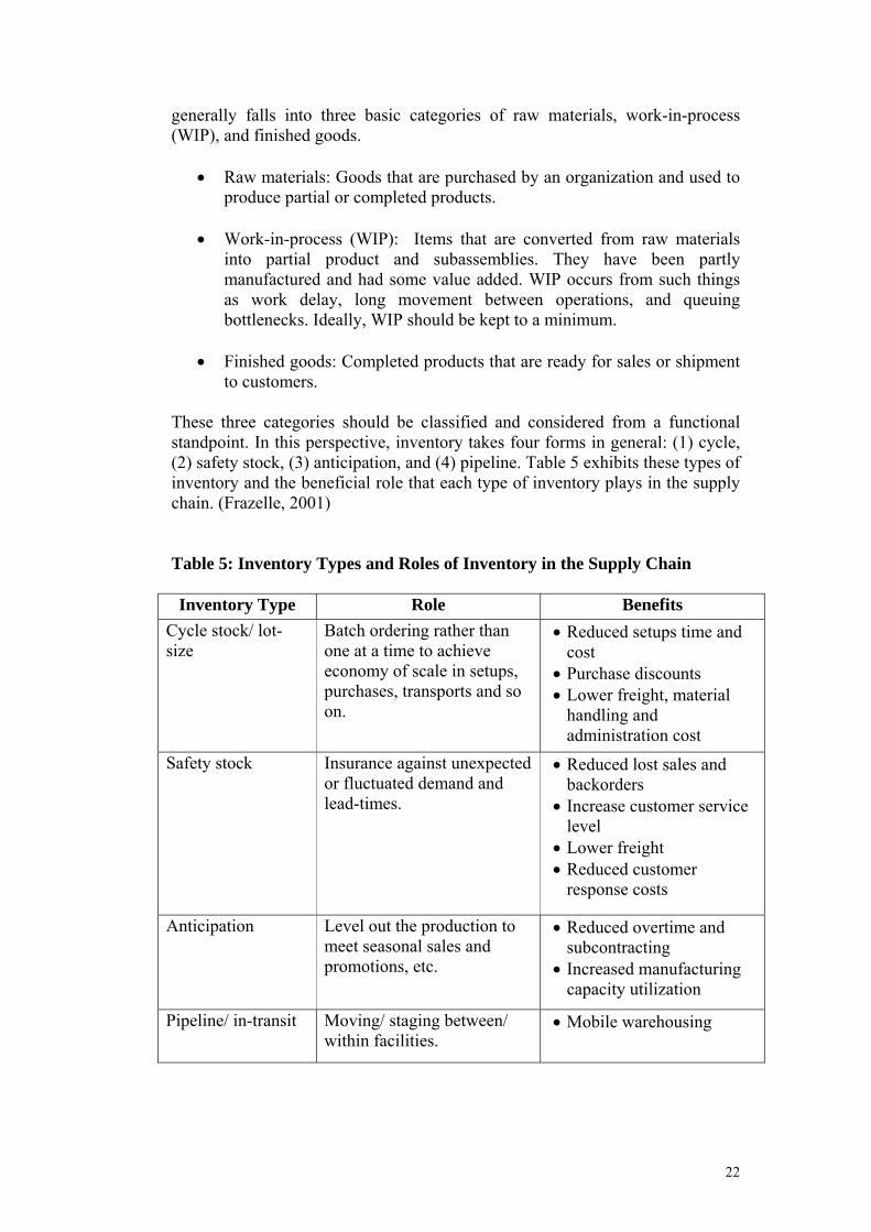
to customers. These three categories should be classified and considered from a functional standpoint. In this perspective, inventory takes four forms in general: (1) cycle, (2) safety stock, (3) anticipation, and (4) pipeline. Table 5 exhibits these types of inventory and the beneficial role that each type of inventory plays in the supply chain. (Frazelle, 2001) Table 5: Inventory Types and Roles of Inventory in the Supply Chain

Inventory Type Role Benefits

Cycle stock/ lot-size

Batch ordering rather than one at a time to achieve economy of scale in setups, purchases, transports and so on.

• Reduced setups time and cost

• Purchase discounts • Lower freight, material

handling and administration cost

Safety stock Insurance against unexpected or fluctuated demand and lead-times.

• Reduced lost sales and backorders

• Increase customer service level

• Lower freight • Reduced customer

response costs

Anticipation Level out the production to meet seasonal sales and promotions, etc.

• Reduced overtime and subcontracting

• Increased manufacturing capacity utilization

Pipeline/ in-transit Moving/ staging between/ within facilities.

• Mobile warehousing

22

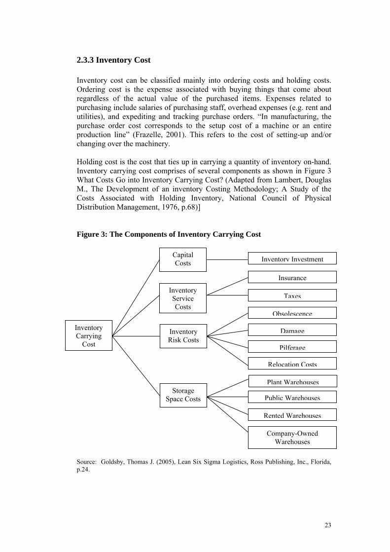
2.3.3 Inventory Cost

Inventory cost can be classified mainly into ordering costs and holding costs. Ordering cost is the expense associated with buying things that come about regardless of the actual value of the purchased items. Expenses related to purchasing include salaries of purchasing staff, overhead expenses (e.g. rent and utilities), and expediting and tracking purchase orders. “In manufacturing, the purchase order cost corresponds to the setup cost of a machine or an entire production line” (Frazelle, 2001). This refers to the cost of setting-up and/or changing over the machinery. Holding cost is the cost that ties up in carrying a quantity of inventory on-hand. Inventory carrying cost comprises of several components as shown in Figure 3 What Costs Go into Inventory Carrying Cost? (Adapted from Lambert, Douglas M., The Development of an inventory Costing Methodology; A Study of the Costs Associated with Holding Inventory, National Council of Physical Distribution Management, 1976, p.68)] Figure 3: The Components of Inventory Carrying Cost

Inventory Carrying

Cost

Storage Space Costs

Inventory Investment

Insurance

Taxes

Obsolescence

Damage

Pilferage

Relocation Costs

Plant Warehouses

Public Warehouses

Rented Warehouses

Company-Owned Warehouses

Capital Costs

Inventory Service Costs

Inventory Risk Costs

Source: Goldsby, Thomas J. (2005), Lean Six Sigma Logistics, Ross Publishing, Inc., Florida, p.24.

23

Capital costs – is the largest factor of inventory carrying cost. As mentioned by Christopher (2005), fifty percent or more of a company’s current assets will often be tied up in inventory. Inventory carrying cost directly reflects the opportunity cost of capital. “The cost of capital is the opportunity cost of investing in an asset relative to the expected return on assets of similar risk” (Krajewski, Ritzman, Maholtra, 2007). What else could you do with the amount of money if it not tied up with inventory? Hence, it is suggested that debt rate, cost of acquiring capital in order to invest in inventory, can be applied to this component. Inventory service costs – Since inventory is regarded as one of assets, thus the property tax rate and an insurance rate to provide coverage against loss and damage to the assets have to be applied in the inventory carrying cost percentage. Inventory risk costs – Highly valuable products have high risk exposure to pilfer and damage, thus they have higher cost attached to them than the lesser valuable items. Storage space costs – is the cost associated with handling inventory and variable storage cost. This cost incur when a firm rents space for storage and it varies due to the change of volume of inventory. It does not include fixed warehousing cost. Since “inventory carrying cost is the most expensive cost in logistics” (Frazelle, 2001), there is the need to analyze the inventory holding cost trade-offs against ordering /set up cost and other supply chain elements. Preferably, they strive to be balanced, having the correct amount of product at the overall lowest cost. It is advised that “an EOQ analysis should be completed as a part of any inventory strategy” (Frazelle, 2001).

• Annual holding cost = Ch(Q/2) Where Q/2 is the average inventory level

• Annual ordering/ setting up cost = Co(D/Q)

Where D/Q is the number of order or setup per year (D = annual usage, Q = lot size in units)

• Total annual cost = Ch(Q/2) + Co(D/Q)

Total annual cost is the function that is to be minimized by choosing appropriate value of Q. Thus, EOQ is derived from the formula of total cost from any lot size Q. “EOQ is a point at which your cost of carrying inventory matches cost of purchasing.” (Muller, 2002)

2 D Co

ChEOQ =

24

• Non-instantaneous Replenishment

The methods discussed above are employed to calculate the total inventory cost and efficient lot size of items purchased from suppliers. However, if the items are produced internally rather than purchased, other methods have to be applied in order to reflect the true cost of work-in-process or finished goods inventory. After the items are produced internally, they can be used or sold as soon as they are completed without waiting until the full lot is completed. Thus, the maximum cycle inventory is defined:

Imax = Q/p (p-d) = Q (p-d/p) Where:

p = production rate per time period d = demand rate per time period If p=d, production would be continuous with no build up of cycle inventory. If p<d, loss of sales opportunities is occurred on an ongoing basis. If p>d, the production rate occur faster than the demand rate, accumulating the cycle inventory and build up p-d units per time period. This build up continues at Q/p until the lot size, Q, has been produced, thereafter, inventory depletes at the constant rate of demand and reaches 0, the next production interval begins. The total annual cost equation for this production situation is:

C = Imax/2 (Ch) + D/Q (Co)

= Q/2 (p-d/p) (Ch) + D/Q (Co) Note: Cycle inventory is no longer Q/2 as it was with the basic EOQ method, but it is Imax/2 In a manufacturing environment, if the setup cost is high, having a large production run is justified as to minimize the total number and costs of setups in exchange of inventory building up as a result of the large production runs. The production run size that minimizes the total setup cost and inventory carrying cost is the economic production lot size (ELS). Based on the cost function, ELS formula is:

2 D Co

ChELS =

p p - d

25

2.3.4 Inventory Control System

The objective of inventory management is to determine the optimized inventory level that is required for any organization to profitably and effectively operate. Basic principle of implementing inventory control system is to manage to have the right item, in the right quantity, at the right place and in the right time. There are several methods of inventory control system that assist you in forecasting the procurement needs. However, in selecting an appropriate inventory control system, a comprehensive knowledge on the nature of demand imposed on inventory items is required. Most inventory fits into one of the above three categories: raw material, WIP, or finished goods, yet the amount of each category varies greatly depends on the specific industry and business. Distribution businesses tend to carry mostly finished goods for resale whereas manufacturing companies tend to have less finished goods and more raw materials and work-in-process (Muller, 2002). Other than the difference of distribution and manufacturing business nature and practices, there is the distinction of demand for the type of inventory they hold. Demand for finished goods, wholesale and resale merchandise, and replacement parts are said to be “independent”, while demand for items, required as components or inputs to a service or product, in manufacturing business are said to be “dependent”. Generally dependent and independent demand, exhibiting different usage and demand patterns, thus must be managed with different techniques. Various inventory control system is selected for a particular application. Some of the prominent systems are shown in Table 6. The suggested systems are not restricted to apply to a specific type of demand; nevertheless the principles of several systems can be melded together. Each system is more effective in some situation than in the others, depending on the product complexity and the systems’ features.

26

Table 6: Inventory Control Systems and Systems’ Features

Type of Demand

Inventory Control Systems Systems’ Feature

Material requirement planning (MRP)

• Product is complex: many level of components

• Lumpy demand with large production batch sizes

• Make-to-order or make-to-stock environments

Drum-Buffer-Rope (DBR) • Capacity is an important issue

• Relatively higher volume with more standardized products

• Assemble-to-order or make-to-stock operation

Dependent

Leans systems

• System is used as a catalyst for continuous improvement

• Production with high volumes and line flows

• Consistent quality, small lot-sizes, flexible workforce, and reliable suppliers

• Assemble-to-order or make-to-stock strategy

Continuous review (Q) system

• Fixed order quantity • Frequently and continuous review

of inventory position • Time between order can vary

Periodic review (P) system • Varied order quantity • Inventory position is periodically

reviewed • Time between order is fixed

Independent

hybrid systems

• Merge features of P and Q systems • Break out into another two system:

optional replenishment and base-stock system

• Independent Demand

Independent demand – replenishment approach – “is influenced by market conditions and is not related to the inventory decision for any other item held in stock” (Krajewski, Ritzmand, Malhotra, 2007). Basically, in independent demand inventory management, the company needs to know how much the ordering quantity is required for each order by calculating the EOQ or lot-sizing and when the order needs to be placed by defining the inventory position where

27

a new order must be made, reorder point (ROP). The objective of ROP rules is high customer service level and low operating costs (Muller, 2002). However, to be able to answer these two questions, we need to identify how the organization reviews their inventory, either on a continuous review (Q system) or a periodic review (P system). Q system has fixed order quantity in which the review of the remaining inventory of an item is done frequently and often continuously to determine whether it is time to reorder, while P system has fixed interval (P) of review where various lot-size or order quantity is made to reach the target inventory level (T) in order to sufficiently cover the expected demand during that fixed interval of review and delivery lead-time. In both systems, yet, safety stock must be set to provide acceptable customer service level for random demand during replenishment lead-times. Q System:

ROP = (Average Demand x Lead Time) + Safety Stock = (D x L) + S P System:

T = Average Demand (Fixed Reviewing Interval + Lead Time) + Safety Stock for the Protection Interval

= D (P + L) + S (P + L) Q system with a fixed order quantity has ROP as a determinant point of when to make a new order. Whenever the inventory level reaches ROP, it signals the need to place a new order. Thus, in Q system, the time between orders may vary depending on when ROP is arrived. However, P System with fixed order interval has T inventory level as a target quantity in making an order. When P period is arrived, the inventory position is reviewed. Hence, in P system, each order quantity or lot-size may be different depending on the inventory level at the time of review. The fundamental difference between Q and P systems is the length of time needed for protection interval, a period over which safety stock must protect the company from running out of stock. A Q system needs stockout protection only during the lead time period because order can be placed as soon as they need and will be received L period later. On the other hand, a P system needs stockout protection for a longer P+L protection interval as orders can be placed only at the fixed intervals and the inventory position is not checked until the next designated review time (Krajewski, Ritzman, Malhotra, 2007). Thus, the total annual cost formula including safety stock is:

Total annual cost = Ch(Q/2) + Co(D/Q) + Ch(S)

• Dependent Demand

Dependent demand – requirement approach – is the demand for items such as raw materials, components and assemblies that is dependent on the demand for

28

the final product. One of the dependent demand inventory control system that has been around for the longest is material requirements planning (MRP). Key elements of MRP:

Master production schedule (MPS) – sets out the quantity of finished products that will be produced within specified period of time.

Bill of materials (BOM) – is the recipe of raw materials, components, subassemblies and so on required to build or to make the finished products. It should specify the quantities required for each part. The objective of MRP is to support the master production schedule. It translates master production schedule into the requirement for all subassemblies, parts and raw materials that needed to produce the required end items. MRP is best used when product is complex that is for a product which has many components which in turn have many components of their own, and so on. (Krajewski, Ritzman, Malhotra, 2007).

29

2.4 Feasibility Study and Investment Analysis

2.4.1 Feasibility Study

According to Small Business Encyclopedia, a feasibility study is a detailed analysis of a company and its operations that is conducted in order to predict the results of a specific future course of action. Small business owners may find it helpful to conduct a feasibility study whenever they anticipate making an important strategic decision. The term of feasibility study is also used to refer to the resulting document. The results of this study are used to make a decision whether or not to proceed with the project (Wikipedia). The feasibility study is also used as an analysis of possible alternative solutions to a problem and a recommendation on the best alternative. The main objective of this feasibility study is to determine whether a certain plan of action is feasible and whether or not it is worth doing economically. This study should focus on the proposed plan of action and also provide a detailed estimate of its costs and benefits in order to assist the management in making the right decision. In this feasibility study, the authors used the investment analysis to clarify and present the costs and benefits between the two project alternatives so that the management can determine on which alternative is the best solution for the company.

2.4.2 Investment Analysis A study of the likely return from a proposed investment with the objective of evaluating the amount an investor may pay for it, the investment’s suitability to that investor (quoted from www.answer.com) There are various methods of investment analysis, for example, cash on cash return, payback period, internal rate of return and net present value which each of them provides some measurement of the estimated return on an investment.

• Cash on cash return The calculation determines the cash income on the cash investment. This method is often used in real estate investment in order to evaluate the cash flow from income-producing assets.

Cash on cash return = Annual Income Total Investment

30

• Payback Period According to real estate dictionary, payback period is refers to the amount of time required for cumulative estimated future income from an investment to equal the amount initially invested. It is used to compare alternative investment opportunities and to measure risk, not return.

Payback Period = Initial Investment Annual Cash Inflows

• Internal Rate of Return Defining in Wikipedia, the internal rate of return (IRR) is a capital budgeting method used by firms to decide whether they should make long-term investments. IRR is used for an investment that requires and produces a number of cash flows over time in which it defines to be the discount rate that makes the net present value of those cash flow equal to zero. Krajewski, Ritzman and Malhopra (2007) stated that with the IRR method, a project is acceptable only if the IRR exceeds the hurdle rate. The IRR is a single number that summarizes the merits of the investment. It can be used to rank multiple projects from best to worst, so it is particularly useful when the budget limits new investments in any year. However, IRR calculates the rate of return of a project without making assumptions about the reinvestment of the cash flows.

• Net Present Value Net present value (NPV) is a standard method for the financial appraisal of long-term projects. The net present value method is used to evaluate an investment by calculating the present values of all after-tax total cash flows and then subtracting the original investment amount (which is already a present value) from their total (Krajewski, Ritzman and Malhopra, 2007). NPV is an indicator of how much value an investment or project adds to the value of the firm. In this feasibility study, the authors used the discounted cash flow analysis, indicating all the cash flows in present value, to evaluate whether which of the alternatives would give the highest present value after subtracting from the total investment amount.

31

Chapter 3: Empirical Study

3.1 Sales Forecast Providing the timeframe of five years (2008 – 2012) to see which of the investment between these two options would generate a better payoff, the sales volume of potting tray has to be forecasted in order to draw on the baseline for decision making and planning in term of finance and operation. Based on the five years forecasted sales volume, the cash flow for these two investment alternatives is projected and will be taken as one of the factors in selecting an appropriate investment decision. In operation aspect, these forecasted sales volumes are required to plan for output levels, materials purchasing, inventories, and long-term capacities (Krajewski, Ritzman, Malhotra, 2007). There are different types of forecasting techniques available, yet to choose the proper forecasting approach depends on the factor of time horizon for the decision requiring forecasts, whether the forecast is for short term, medium term or long term. A forecasting of five years sales volume of potting tray is considered as long-term (more than 2 years) forecast. Two long-term forecasting methods are suggested: judgment method and causal method. Judgment methods, the only qualitative forecasting methods among the others, translate opinion of managers and experts, consumer surveys, and salesforce estimated into quantitative estimates. Judgment methods are exploited when there is inadequate historical data to possibly make forecast from quantitative methods. However, in this case, given the monthly historical sales data of 2006 and 2007 and the projected monthly sales volume of 2008 by KT Plastics (shown in Table 7), the annually forecasted sales volume of potting tray can be projected for the next four years (long term) by using casual method: linear regression, a best known and most commonly used causal method.

Table 7: Sales Volume of Potting Tray

Sales Volume (units)

Month/Year 2006 2007 Projected Sales 2008

Jan 4,800 2,600 5,200 Feb 4,800 7,100 14,200 Mar 4,500 10,900 21,800 Apr 600 3,700 7,400 May 1,000 10,000 20,000 Jun 2,700 6,300 12,600 Jul 7,200 25,100 50,200 Aug 6,400 23,400 46,800 Sep 3,300 14,500 29,000 Oct 8,600 15,400 30,800 Nov 12,200 20,400 40,800 Dec 7,700 25,300 50,600 Total 63,800 164,700 329,400

32

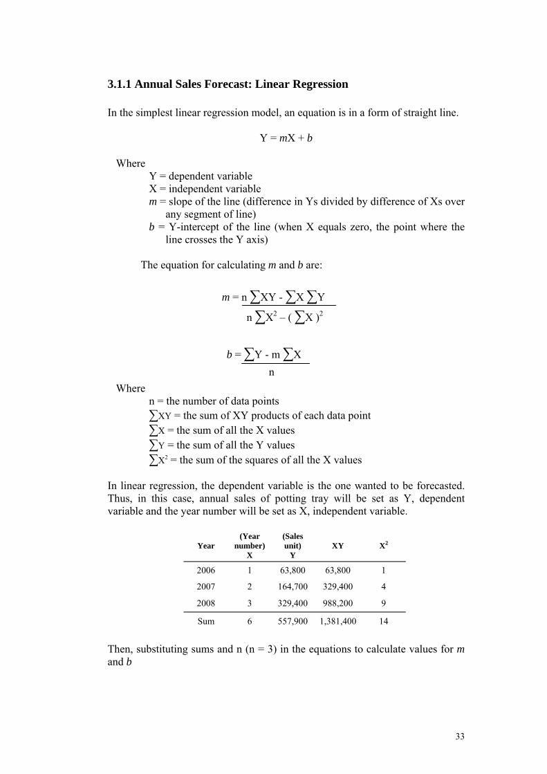
3.1.1 Annual Sales Forecast: Linear Regression

In the simplest linear regression model, an equation is in a form of straight line.

Y = mX + b

Where Y = dependent variable X = independent variable

m = slope of the line (difference in Ys divided by difference of Xs over any segment of line)

b = Y-intercept of the line (when X equals zero, the point where the line crosses the Y axis)

The equation for calculating m and b are:

m = n ∑XY - ∑X ∑Y

n ∑X2 – ( ∑X )2

b = ∑Y - m ∑Xn

Where n = the number of data points ∑XY = the sum of XY products of each data point ∑X = the sum of all the X values ∑Y = the sum of all the Y values ∑X2 = the sum of the squares of all the X values

In linear regression, the dependent variable is the one wanted to be forecasted. Thus, in this case, annual sales of potting tray will be set as Y, dependent variable and the year number will be set as X, independent variable.

Year (Year

number) X

(Sales unit)

Y XY X2

2006 1 63,800 63,800 1

2007 2 164,700 329,400 4

2008 3 329,400 988,200 9

Sum 6 557,900 1,381,400 14

Then, substituting sums and n (n = 3) in the equations to calculate values for m and b

33

m = 3(1,381,400) – 6(557,900)

3(14) – (6)2

= 132,800

b = 557,900 – 132,800(6)

3 = -79,633.33 Therefore, the line equation that best fits these data is:

Y = 132,800 (year number) – 79,633.33 To predict sales volume (Y) for next year 2009, simply put the year number (4th year) into the equation and continue until 2012 sales volume (7th year) is derived. Five years (2008-2012) forecasted sales volume for potting tray is shown in Table 8. Table 8: Five Years Forecasted Sales Volume for Potting Tray

Year (Year

number) X

(Sales Unit)

Y

Rounded Units

2008 3 329,400 329,400 2009 4 451,567 451,600 2010 5 584,367 584,400 2011 6 717,167 717,200 2012 7 849,967 850,000

3.1.2 Monthly Sales Forecast: Seasonal Patterns

Having the annual sales volume might be sufficiently desirable to compute and analyze the cash flow for investments, however, to have a prudent planning in an operational level and to increase the forecast accuracy; monthly demand of a product is rather considerable. Hence, based on the forecasted annual sales volume of potting tray, a demand for each month during year 2009-2012 can be forecasted and projected. As advised by KT Plastics, the demand of potting tray is regarded as seasonal, regularly repeating upward and downward movement in a year. Annually, demand tends to have an upward movement in the back half of the year starting from July onwards, due to the beginning of planting season, particularly for rubber trees. To forecast seasonal pattern of demand in each year, the multiplicative seasonal method is used to calculate the monthly demand of potting tray. In multiplicative seasonal method, the seasonal indices are multiplied by an estimate of average demand to derive the seasonal forecast. The calculation procedures and illustration are shown below.

34

35

(i) For each year, calculate the average demand per season by dividing

annual demand by the number of seasons per year. (ii) To find the seasonal index for a season in each year, divide the actual

demand for a season by the average demand per season. (iii)Calculate the average seasonal indices by sum up the seasonal indices for

a season and divide by number of year of data. (iv) To obtain the seasonal forecast for next year, it requires two steps here.

Firstly, divide the forecasted annual demand by the number of season per year, yielding the average demand per season. Secondly, multiply the average seasonal index for a season by the average demand per season, obtaining the seasonal forecast for that particular year.

Step: (i), (ii), (iii)

2006 2007 2008

Month/Year Sales Volume (A)

Seasonal Index (1)

Sales Volume (B)

Seasonal Index (2)

Projected Sales Volume (C) Seasonal Index (3)

(iii) Average Seasonal Index (1)+(2)+(3)/3

Jan 4,800 0.90282 2,600 0.18944 5,200 0.18944 0.427231 Feb 4,800 0.90282 7,100 0.51730 14,200 0.51730 0.645810 Mar 4,500 0.84639 10,900 0.79417 21,800 0.79417 0.811579 Apr 600 0.11285 3,700 0.26958 7,400 0.26958 0.217338 May 1,000 0.18809 10,000 0.72860 20,000 0.72860 0.548428 Jun 2,700 0.50784 6,300 0.45902 12,600 0.45902 0.475290 Jul 7,200 1.35423 25,100 1.82878 50,200 1.82878 1.670597 Aug 6,400 1.20376 23,400 1.70492 46,800 1.70492 1.537866 Sep 3,300 0.62069 14,500 1.05647 29,000 1.05647 0.911207 Oct 8,600 1.61755 15,400 1.12204 30,800 1.12204 1.287212 Nov 12,200 2.29467 20,400 1.48634 40,800 1.48634 1.755783 Dec 7,700 1.44828 25,300 1.84335 50,600 1.84335 1.711660 Total 63,800 (ii) (A) / 5,316.67 164,700 (ii) (B) / 13,725 329,400 (ii) (C) / 27,450 (i) Average demand/season

63,800/12 = 5,316.67 164,700/12 =

13,725 329,400/12 = 27,450

36

37

Step: (iv)

Year

(A)

2009 (B)

2010 (C)

2011 (D)

2012 Annual Forecast (Sales in units) 451,600 584,400 717,200 850,000

Average demand per season 451,600/12 = 37,633 584,400/12 = 48,700 850,000/12 = 70,833 717,200/12 = 59,767

Monthly Demand Forecast

Month

(E) Average Seasonal

Index

2009 (A) x (E)

2010 (B) x (E)

2011 (C) x (E)

2012 (D) x (E)

Jan 0.42723 16,078 20,806 25,534 30,262 Feb 0.64581 24,304 31,451 38,598 45,745 Mar 0.81158 30,542 39,524 48,505 57,487 Apr 0.21734 8,179 10,584 12,990 15,395 May 0.54843 20,639 26,708 32,778 38,847 Jun 0.47529 17,887 23,147 28,406 33,666 Jul 1.67060 62,870 81,358 99,846 118,334 Aug 1.53787 57,875 74,894 91,913 108,932 Sep 0.91121 34,292 44,376 54,460 64,544 Oct 1.28721 48,442 62,687 76,932 91,177 Nov 1.75578 66,076 85,507 104,937 124,368 Dec 1.71166 64,415 83,358 102,300 121,243 Total 451,600 584,400 717,200 850,000

3.1.3 Forecast Accuracy As forecasting is a process of estimation in unknown situations, forecasts are never perfect, yet are valuable to better in preparation for actual demand. Accurate and timely forecast is a vital component of business operation. Since demand forecast accuracy is critical for proper planning and allocation of resources, it is crucial to measure the forecast errors in order to see how accurate the forecasts are and thus able to adjust the forecasting method accordingly to reduce the gap of error. Forecast error is the deviation of the forecasted quantity from the actual, in which the forecast accuracy is the converse of error.

As the average forecast error for a time series of forecasts for potting trays need to be observed, the mean absolute percent error (MAPE) is used to measure the accuracy of the value in the forecasted points in time and is expressed as a percentage error so that the error of each time series that differ in level can be compared.

The forecast accuracy is needed to be measured constantly either on a yearly, quarterly, or ,ideally, on a monthly basis so that the company can see whether the current forecasting method is fitting and can provide the forecasted figures as close as the actual, in which it gives an acceptable level of error. From the historical sales data of 2006 and 2007, only the actual sales volumes were given, but none of the forecasted figures were documented and thus no forecast errors were measured. The 2008 forecasted sales volume is given by the company based on management opinions and experiences, judgment method, due to a campaign of growing rubber trees promoted by Thai government, the special upcoming event on this year. As of now, the MAPE of 2008 forecast can be calculated only until April, based on the available actual sales data.

38

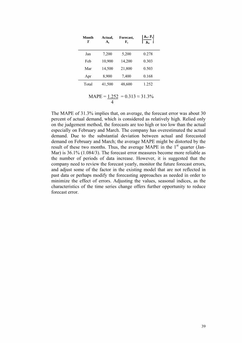
Month T

Actual, At

Forecast, Ft

Jan 7,200 5,200 0.278

Feb 10,900 14,200 0.303

Mar 14,500 21,800 0.503

Apr 8,900 7,400 0.168

Total 41,500 48,600 1.252

MAPE = 1.252 = 0.313 ≈ 31.3%

4 The MAPE of 31.3% implies that, on average, the forecast error was about 30 percent of actual demand, which is considered as relatively high. Relied only on the judgement method, the forecasts are too high or too low than the actual especially on February and March. The company has overestimated the actual demand. Due to the substantial deviation between actual and forecasted demand on February and March; the average MAPE might be distorted by the result of these two months. Thus, the average MAPE in the 1st quarter (Jan-Mar) is 36.1% (1.084/3). The forecast error measures become more reliable as the number of periods of data increase. However, it is suggested that the company need to review the forecast yearly, monitor the future forecast errors, and adjust some of the factor in the existing model that are not reflected in past data or perhaps modify the forecasting approaches as needed in order to minimize the effect of errors. Adjusting the values, seasonal indices, as the characteristics of the time series change offers further opportunity to reduce forecast error.

39

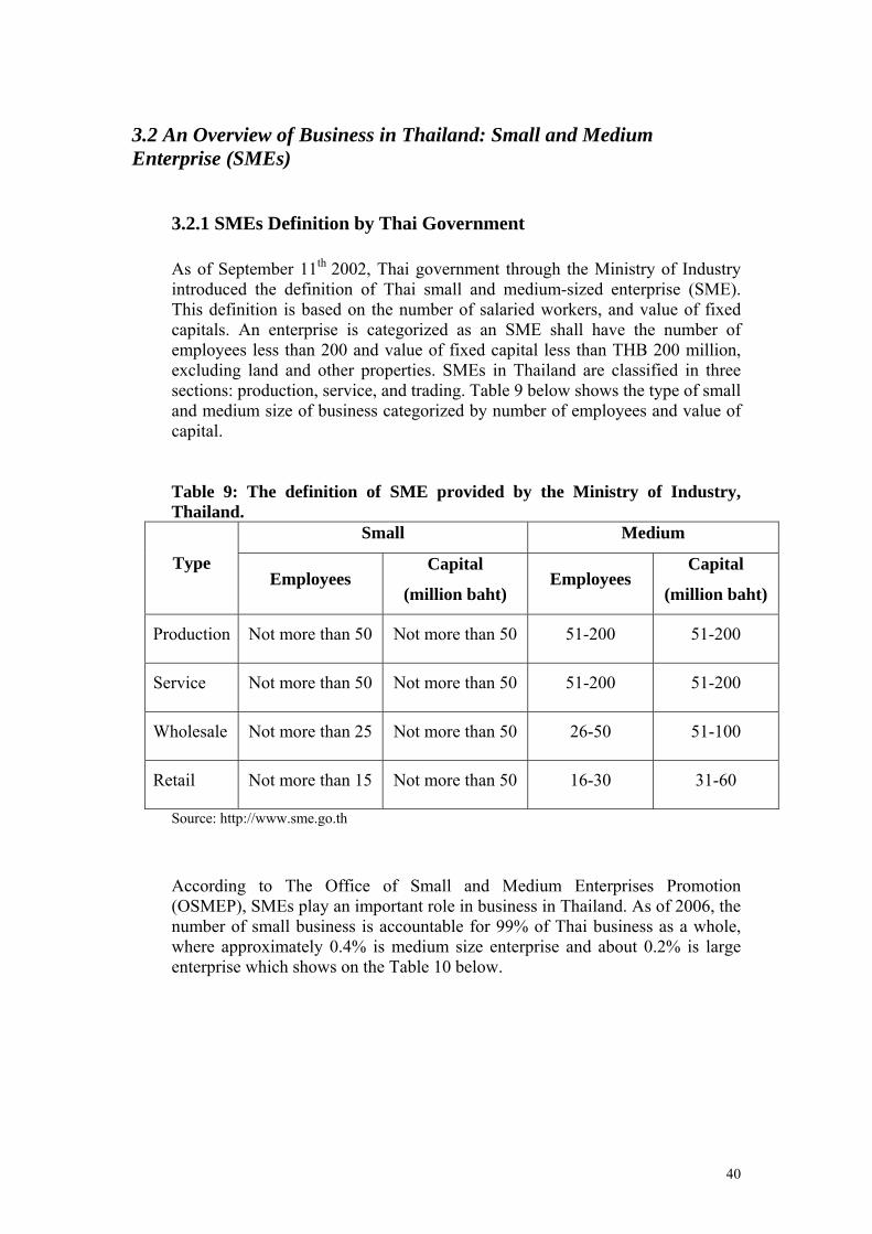
3.2 An Overview of Business in Thailand: Small and Medium Enterprise (SMEs)

3.2.1 SMEs Definition by Thai Government

As of September 11th 2002, Thai government through the Ministry of Industry introduced the definition of Thai small and medium-sized enterprise (SME). This definition is based on the number of salaried workers, and value of fixed capitals. An enterprise is categorized as an SME shall have the number of employees less than 200 and value of fixed capital less than THB 200 million, excluding land and other properties. SMEs in Thailand are classified in three sections: production, service, and trading. Table 9 below shows the type of small and medium size of business categorized by number of employees and value of capital. Table 9: The definition of SME provided by the Ministry of Industry, Thailand.

Small Medium

Type Employees

Capital

(million baht) Employees

Capital

(million baht)

Production Not more than 50 Not more than 50 51-200 51-200

Service Not more than 50 Not more than 50 51-200 51-200

Wholesale Not more than 25 Not more than 50 26-50 51-100

Retail Not more than 15 Not more than 50 16-30 31-60

Source: http://www.sme.go.th

According to The Office of Small and Medium Enterprises Promotion (OSMEP), SMEs play an important role in business in Thailand. As of 2006, the number of small business is accountable for 99% of Thai business as a whole, where approximately 0.4% is medium size enterprise and about 0.2% is large enterprise which shows on the Table 10 below.

40

Table 10: Structure of business in Thailand categorized by size

Size of Business

Total Number of

business As of 2004

Total Number of

business As of 2005

Total Number of

business As of 2006

Percentage of

2006

Unable to categorize size 6,209 6,210 8,240 0.4

Large Enterprises (LEs) 4,311 4,474 4,292 0.2

Small and Medium Enterprises (SMEs) 2,199,130 2,239,069 2,274,525 99.4

• Medium Enterprises (MEs)

10,036 10,493 9,791 0.4

• Small Enterprises (SEs)

2,189,094 2,228,576 2,264,734 99

Total 2,209,650 2,249,753 2,287,057 100 Source: http://www.sme.go.th SMEs play a very crucial role to the economies of many emerging nations from the viewpoint of generating employment and economic growth. (Koh et al., 2007) OSMEP has promoted and supported those SMEs in order for them to effectively manage its own business. Supply chain management is taking into account when company need to improve and manage their operations more effectively.

Supply chain management (SCM), according to the Council of Supply Chain Management Professionals (CSCM), encompasses planning and management of all activities involved in sourcing and procurement, conversing all logistics management activities as well as coordinating and collaborating with channel partners, who are suppliers, intermediaries, third party service providers, and customers. In essence, supply chain management integrates supply and demand management within and across companies.

SCM and related strategies are very significant to the success of manufacturing firm. This is because the cost and quality of goods and services sold are directly related to the cost and quality of goods and services purchased. (Koh et al., 2007) As suggested by Zeng (2000), an organization’s profitability is determined, in a large extent, by its purchase or sourcing. Thus, sourcing strategically has been considered as one of the key drivers for the company survival and growth. Villa (1998), stated that the adoption of appropriate production sourcing strategies and buyer-supplier relationships is not only confined to large enterprises (LEs), as a great number of small and medium sized enterprises (SMEs) also actively take this into consideration. However, there are many differences between small and large enterprises. Small firms enjoy the advantage of great flexibility and high level of efficiency. They can be very innovative and need not bound in the complicated organization structures.

41

On the other hand, small firms are severely constrained by their lack of funds and limited resources. Due to their size, they may have less power in their dealing with large organizations. (Tam et al., 2007) With limited resources in both personnel and capital, there is a need for SMEs to concentrate on their core business and thoroughly concern on the investment matters. Thus, outsourcing has recently come to their attention. Outsourcing is one of supply chain management strategies that SMEs should add to their business strategies.

42

3.3 Previous outsourcing According to our investigation, throughout the outsourcing periods, the company has changed to three outsourced suppliers in total with the last supplier still remains as a current supplier. To determine the advantages and disadvantages of outsourcing, the check list has been applied in order to compare and point out the reasons behind the decision making, and also discuss on what went wrong, in which they became disadvantages that the company decided to backsourcing. Potting tray production line consists with two main processes. First is the processing of plastics through extrusion machine to get plastic sheets and second is the processing of plastic sheets through thermoforming machine to obtain potting trays. At the beginning, the company outsourced both processes to outside party. In practice, when the customer hire a supplier to manufacture a product with customized specification, the customer has to design and order to make their own mold to use with supplier’s thermoforming machine in order to produce the finished product according to their specification. The mold is given to the supplier so that they can supply and fulfill customer’s order, though legally, it is the property of the customer who actually design and own it. Thus there is a certain risk that the supplier would use the company’s mold to produce similar product and sell to the market itself rather than to only supply to customer as per orders. However, the relationship between the company and outsourced supplier is solely based on trust. As stated by Blois (1992), trust is the acceptance of vulnerability. Its function is to reduce social complexity in two ways: firstly, in the present and as we look to future, to reduce our sense of vulnerability as potential contingencies is regarded and secondly, as we currently assess the future by increasing our confidence that other will act proactively in case where the need to adapt to contingencies arises. The company believes that trust can, therefore, be an important factor in business relations, which makes cooperation more flexible. One of the reasons that company chose outsourcing rather than direct investment was because the company can enjoy the benefit of increasing speed and shorten time to market. Since the company was new in manufacturing, outsourcing was the way to reduce risk and access to experts and specialists. However, the problem arose when first contracted supplier could not comply with the standard which they were promised, the company, therefore, had to find another supplier for this product. Second contracted supplier is the manufacturing in another business section. Their main products are beauty accessories, yet they have the machine that is capable of producing the potting trays. The supplier’s production quality and price were acceptable. Nevertheless, as the business size of both parties is small enterprise, a written contract was neglected. During that time, there were several reasons supporting the outsourcing decision. One reason was that investing in new production line required the company a certain period of time to pass through the learning curve, and thus might not be able to response to the customers’ demand and needs in a timely manner. Also, at that time, there was another requirement, the expansion of the production line of core product,

43

mulching film, arose simultaneously. Since the company had limited space to do both expansion and building up of the new production line, thus the company with limited resources decided to allocate the available space to the core business function. Not long after the company outsourced to the second supplier, some problems occurred. The supplier could not fulfill the product quantity as per orders; consequently, leading the company to make delayed delivery to their customers. Due to the business nature of agricultural industry, the product is quite common and the gap of price difference is not so big. Hence, customers would not wait for delayed product. If the company cannot fulfill the orders accurately, the company is likely to lose the customer to its competitors. Nevertheless, after investigated, the company found out that this second supplier became the company’s indirect competitor as they also supplied the potting trays using the company’s mold to another trader who is the company’s main competitor. In the end, getting the mold of potting tray back, the company terminated business with this supplier, and found another supplier. Third contracted, current supplier is a manufacturer in the market which is quite closed and related to the company’s business market. The main reason of selecting this supplier is based on price and quality of product. Similar to the first two suppliers, there is only a verbal agreement. Due to the size and nature of business, SMEs in Thailand rarely make a written contract. Despite of the loss of some business to the competitor because of the formal suppliers who sold the products to the company’s competitor, the company is able to acquire back its customers through the price competitiveness offering by this current supplier. However, the problem again arises when the order quantities are dramatically increased as the company is able to expand to new market area. Since then, the supplier’s deliveries started to delay. Moreover, the company realizes that the supplier has sold the potting trays produced by the company’s mold to the customers in the same market, and again turns to be the company’s direct competitor.

Table 11: The reason for outsourcing

Reason for outsourcing Supplier A Supplier B Supplier C • Price competitiveness • Reduce capital expenditures • New for manufacturing • Lack of knowledge • Access to experts and specialists • Greater flexibility • Focus on core competency • Increase speed and shorten time to market • Increase ability to meet changing market need • Reduce risks • Resource not available internally • Lack of space for new production line • Ability to reduce inventory stock • Supplier is in different business sector

X X X X X

X X

X X X X X X X X

X

X

X X

X X X X X

X

X X

**See appendix I

44

From these problems of outsourcing, the company, therefore, considers to backsourcing potting tray production from its current supplier. Backsourcing is pulling a function back in-house as an outsourcing contract expires. According to the outsourcing-law, backsourcing is the expiration or termination of an outsourcing arrangement and the recapture in-house of the outsourced function. After the company faced with several problems occurring due to outsourcing, the company needs to consider more carefully in order to reduce the risk that might happen either on finding a new supplier for process that need to be outsourced (option 1) or investing to backsource the whole production line in house (option 2). There are several frameworks that need to be included when making the sourcing decisions. Four key questions are used to demonstrate and identify the core competencies. Figure 4: Four Key Questions to Consider in Identifying a Core Competency

No

Yes

Yes

No

Do not outsource unless provider can ensure same/better performance as current.

Difficult to replicate

Does it contribute significantly to customer’s perceived value?

No Consider outsourcing

Consider outsourcing. Proceed with caution: outsourcing must be transparent to customer.

No

Yes Yes Do not outsource

Difficult to replicate

Does it directly support a critical value-added skill set?

Source: Fawcett, Ellram and Ogden (2007), Supply Chain Management: From vision to implementation, Pearson Prentice Hall, New Jersey, p. 282. Figure 4 above shows that the company can consider outsourcing because the production line is easy to replicate and significantly contributed to the customer’s perceived value. However, based on the company’s experience, other business aspects must be also taken into consideration. Since the company’s suppliers have a tendency

45

to become competitors, a legitimated contract and/or a building of long-term relationship with suppliers must be established so that outsourcing can offer benefit opportunities to the company rather than threats. Nevertheless, the company might not be able to conclude for a solution from these four questions, which only identify the core competencies of the company. A conceptual framework for evaluating the make or buy decision proposed by McIvor (2000) combines with some other tools used by Fill and Visser (2000), a composite approach to the make or buy decision, has been employed in order to help top management obtaining a clear vision of both qualitative and quantitative aspects of the make or buy decision. McIvor, Humphreys and McAleer (1997), defined framework into four stages which are;

• Stage 1: Define the core activities of the business • Stage 2: Profile the appropriate value chain links • Stage 3: Total cost analysis for core activities • Stage 4: Analysis of potential suppliers for partnership

3.3.1 Stage one: Define the core activities of the business

In this stage, to define the company’s core product, in term of selling and manufacturing, mulching films is one of the company’s core products. Potting trays is another product that the recent sales volume increases dramatically. The company forecasts that the upward trend of its sales will continue for several years because Thai government has recently promoted the growing of rubber trees.

The nine questions guideline proposed by Ewaltz in 1991 which used in the composite outsourcing decision by Fill and Visser (2000) is applied in order to help the company to consider the structural aspects associated with the decision and, in particular, to focus on how integrated the organization should be. This set of questions is asked in order to clarify the decision making of whether to buy or to make. 1. How unique are the production processes? Potting tray production processes consist with two main machines, extrusion machine and thermoforming machine. The production line is possible to produce variety of products that differentiate by the use of mold. Potting trays which sell in the market may have various sizes, but there are two sizes: 104 and 72 holes that are widely used in the market depending upon the seed they are growing. Even though the production processes are commodity oriented, the core competency of these production processes, showing the product’s uniqueness and differentiation, is at the process done by thermoforming machine. Thus, it is

46

possible to outsource material which is processed from extrusion machine and have an in-house processing of thermoforming machine. Conclusion: in-house the process of thermoforming machine and outsourcing the process on extrusion machine. 2. How severe are the market cycles? And how frequent? The market cycle is depending upon the season. Normally, high season starts from June until February the following year. While September to November is peak season, the gap between peak and low season makes the sale of all products fluctuated due to the growing season of each type of plants. Demand swings required the resources to work overtime over the second half of the year; therefore, costs advantage can be gained from the economies of scale. Since this production line requires only a few workers, thus it can also employ workers from other production lines such as mulching films and plastic bags during the time when it is considered as the off-peak period for these products. In case of hiring new workers, during the low season of potting tray, labor can be transferred to work in other production line. Conclusion: either in-house or outsourcing 3. Just how much capital does internal manufacturing require? To fully have the potting tray production line done in-house, the company requires investing in two machines: extrusion machine and thermoforming machine. The overall investment amount for these two machines is approximately THB 6,000,000. However, there is another available option for the company, choosing to invest in one machine which is thermoforming machine (core-processes) and outsourcing the process of extrusion machine. The investment in one machine, thermoforming machine, requires approximately TBH 2,050,000. The return on investment (payoffs) which will show later in this report shows that the return rate is expected to be higher than the discounted rate. Conclusion: in-house 4. How does geographic dispersion of customers influence resourcing

decisions? The geographic dispersion of customer does not influence the resourcing decisions since most of the manufacturers are located around Bangkok and the delivery to customer is mostly done through transportation company, in which in this case customer will pay for transportation costs. Conclusion: not affect the decision

47

5. Does the market expect the firm to be a manufacturer? The firm can be either a manufacturer or a trader but the most important issue is price competitiveness. Some of the customers such as seed companies expect the company to be the manufacturer of the product because it is easier to track down when something goes wrong. Conclusion: in-house. 6. How long will the process be viable? The process of setting up the production line will be taken around two months due to ordering lead-time of new machines. Yet, if company can find supplier that can provide used machines, this production line can be set up immediately. The company has long establishment of relationship with suppliers of plastic raw materials, thus the problem of sourcing raw materials can be eliminated. In case, if the company would like to invest in thermoforming machine and outsourcing the process of extrusion machine, sourcing of plastic sheets’ suppliers (output from extrusion machine process) would not be a problem as well as the company already has the number of qualified plastic sheets’ suppliers on hand. Due to the fact that the company is now outsourcing this product, potting trays, the time consumption in setting up this new production line will not cause a problem of shortening of product supplies to market. However, the delay would only cause the company to lose some profit from the gap of producing cheaper in-house than the current outsourcing. Conclusion: in-house. 7. Are these suppliers capable of doing the work, in terms of both technology

and capacity? The current supplier of potting trays is capable of supplying the product for the company, but there are several issues that company concerns about, which involves the issue of direct competition. Suppliers might become competitors in the future since there were some signs showing that the suppliers are willing to enter the market and to take over some shares in the market. Acquiring back the processes in-house might even force the supplier to be the company’s direct competitor. But, on the other hand, if the company takes all the processes in-house, the company can enjoy the advantage of lower production costs. Conclusion: in-house.

48

8. Are there idiosyncrasies in the product, the manufacturing processes, or the

market that force a sourcing decision? Every manufacturers, who have these machines: extrusion and thermoforming machine, can produce similar products, particularly plastic sheets output, processing through extrusion machine. However, the unique attributes and/or differentiation of the product are depended on the design of mold used to produce each product in thermoforming machine. Thus, the process of thermoforming machine is considered as a core process of this production line. Conclusion: in-house thermoforming machine process. 9. Can the corporate culture be changed? This is hard to conclude. However, it might be difficult for the company to change in some way such as having a legitimate contract to control over their suppliers since it is not a norm of business practice for Thai SMEs. The company itself is also a family own business in which it needs high flexibility in business operation and has quite a loose control within an organization. Conclusion: in-house. From these nine questions, the production of potting tray shall be taken back in-house and potting trays will become one of the core products of the company since the company sees an opportunity to highly increase sales in market. However, within the decision of acquiring back this production line, the company must again decide on whether to invest on the whole production line or invest on only the core process which stated in question number eight. Hence, if the company decides to do all processes in-house, the company needs to invest in two machines: extrusion machine and thermoforming machine. If only the core process is to be done in-house, the company needs to purchase only thermoforming machine and outsource plastic sheets from supplier. Yet, to be able to finalize the conclusion, the evaluation of cost and profit for each option has to be examined.

3.3.2 Stage two: Profile the appropriate value chain links

In this stage, KT Plastics must evaluate the company’s capabilities in relation to both of suppliers and competitors. In potting tray market, there are a few companies that are both manufacturing and distributor. Most of the competitors in the market are trader or distributor. Based on the different levels of complexity and specificity which identify the four different types of the main characteristics of outsourcee-outsourcer relationships, the company and its supplier is the traditional vendor level with low complexity and low specificity. The relationship between these types of outsourcee-outsourcer has an objective

49

on resolution to an immediate problem. For the traditional vendor, term of relationship is usually depended on the quality, productivity and price competitiveness offered by the suppliers. Figure 5: Type of Relationships between Outsourced-Outsourcer Based on Different Levels of Complexity and Specificity

spec

ifici

ty

Low

Low

Traditional Vendor

High

High

Network Organization Traditional Relationship

Strategic Union

Complexity

Source: Franceschini and Galetto et.,al (2003), Outsourcing: guidelines for a structured approach, Benchmarking An International Journal, Vol. 10 No. 3, pp. 246-260. At the moment, the company does not produce in-house, but the sloppy control over its supplier giving the risk of losing some market shares as the supplier can sell this same product to the company’s competitors or customers. For the value chain links, the materials suppliers have a relatively close relationship with the company since they already supply the materials to other production lines, and also the company can access to their expertise on materials’ details and specifications. Having new production processes in-house, though the company has no technical knowledge and skills in operating the new machines, the company will receive the training from the machine vendor. Taking back production processes of potting tray in-house provides an opportunity to lowering production costs while the company might have to face with current supplier become direct competitor. Although the new players can enter into the market, to gain large shares in the market would take them sometimes as the customers give the significance in business relationship to a certain degree. Despite of the competitor (current supplier) using the price competition to gain more shares, having this production line in-house would contribute the price competitiveness to the company. The company also believes that the production cost would not be different from its current supplier’s.

50

3.3.3 Stage three: Total cost analysis of core activities

This stage involves measuring all the actual and potential costs related in sourcing activity – internally and externally. With the nature of SMEs business, it might be difficult, in some point, to measure all costs associated throughout the entire supply chain. It is quite complex to have a detailed calculation for each cost such as ordering costs, warranty claims, collaborating costs and so on separately. Thus, in this circumstance, this stage will not encompasses all cost associated with the acquisition of all activities throughout the entire supply chain. Yet, the calculation will only base on the estimation of investment for the new production line and the costs of production of potting tray, comparing with the purchased price from supplier. Additional details of costs calculation will show later in this report in the sections of inventory cost and quantitative analysis. In this stage, estimated calculation of the product cost per unit is applied in order to compare the cost of producing in-house and outsourcing price. Material costs, fixed costs (labor and utilities), depreciation and packaging costs are calculated in order to have estimated price of product per unit. The material cost is based on current material price (as of February 2008), where fixed cost is calculate by the costs of labor and utilities. While depreciation is calculated by the method of tax system in Thailand, considering the salvage value of machine to be equal to zero by the end of year five. Annual working day for the company is 300 days, while the productivity of this production line is approximately 2,150 units per day. Table 12: Estimate cost calculation for potting tray (per unit)

Outsourcing purchased price

Investment only in thermoforming

machine

Investment in whole production

processes Materials costs - 8.99 5.89 Fixed Costs (Labor & Utilities) - 1.12 1.86

Depreciations - 0.64 1.72 Packaging - 0.15 0.15 Total cost / unit THB 11.50 THB 10.90 THB 9.62

Table 12 above shows the comparison price between outsourcing and in-house production where the production cost of two options for in-house production is also given in order to identify the feasibility and opportunity in the investment and to find the estimated price of these three options. Outsourcing purchased price costs THB 11.50 per unit while investment only in thermoforming machine costs THB 10.90 to produce a potting tray. The lower production cost allows the company to gain more profit from the gap of buying and producing.

51

If the company decides to investment for the whole production line, company will have the lowest price per unit for potting tray at THB 9.62. For an overview of investment and production costs shown in this stage, there is the feasibility for the company to invest and backsourcing this production line in-house. The price comparison points out that the company should invest in-house in order to gain the price advantages. In this case, as the company is currently outsourcing this function, the company may wish to acquire it back in the company. However, there are other factors that need to take into consideration regarding the investment on machinery such as cash flow analysis, break-even analysis, decision tree analysis which will be discussed later in this paper.

3.3.4 Stage four: Analysis of potential suppliers for partnership

As of this stage, outsourcing the whole production processes is not advised, according to the earlier stages of analysis. Thus, there are only two concerns left: either to wholly produce in-house or to outsource plastic sheets process to outside supplier. In this stage, the company needs to consider whether there are any potential plastic sheets suppliers, who are qualified for a partnership relationship, if the company chooses to outsource this process. As mentioned earlier, the company knows a number of suppliers who can be a qualified supplier of plastic sheets. Nevertheless, only after the qualitative and quantitative aspects have been analyzed completely, the decision in this stage can be finalized. The model describes the use of four stages analysis to help the company to formulate an effective make or buy decision. The purpose is to alert the management to consider the strategic issues along with the cost analysis. It is crucial to identify the company’s core processes as the failure to identify these core activities might lead the company to face high risk in the future. A number of questions are used for gathering information in order to avoid the risk of outsourcing core processes. From the interview using nine guidelines question, it shows that the core process of the potting tray production line is the process that using thermoforming machine to form plastic sheet into potting tray shape. If company decides to backsourcing the potting trays production from its supplier, the company may consider outsourcing plastic sheets process to outside maker while keeping the product’s shape forming process by thermoforming machine to do in-house. By profiling in the value chain links, the company can decide on appropriate strategic relationship with supplier. A well combination of management consideration and judgment in cost analysis assists the company to have a clear and adequate information requirement for the make or buy decision.

52

3.4 Inventory Application To establish a new production line for a product, potting tray, KT Plastics has to make decision on the two alternatives: either outsource half process or fully produce in-house. Analyzing the cost of inventory for these two options is one of the parameter used for decision making. In addition, regardless of choosing either of these two options, knowing the efficient quantity of inventory is essential and considered to be valuable in maintaining customer demand and satisfaction. Yet, in the end, the efficient production lot-size can be used to compute the time between production runs and time required to process the efficient lot-size, comparing the ratio of these two values to indicate the utilization rate of machine and resources. Option 1: Partly outsource KT Plastics would have the supply of plastic sheet rolls from supplier and take them to process further in a thermoforming machine to get the potting trays. Raw Material Finished Goods Option 2: Fully made in-house KT Plastics receives plastic supply from suppliers and have them process through plastic extrusion machine to get a roll of plastic sheets, subsequently, having this plastic sheet go through a thermoforming machine to form the potting tray. Raw Material WIP Finished Goods

Plastic sheet in a roll

Potting trays

Plastic sheet in a roll

Potting trays Thermoforming

M/C

Thermoforming M/C

Plastic Extrusion M/C

Plastics: PS & black

3.4.1 Sales Forecast and Demand Simulation

Since this production has not yet been in place, demand simulations are created in Excel Spreadsheet (see Appendix II: A & B) in order to determine the level of inventory required for these five years (2008-2012).

53

Table 13: Monthly Forecasted Sales Volume of Potting Tray (in units)

Year/ Month

Projected Sales 2008

Forecasted 2009

Forecasted 2010

Forecasted 2011

Forecasted 2012

Jan 5,200 16,078 20,806 25,534 30,262 Feb 14,200 24,304 31,451 38,598 45,745 Mar 21,800 30,542 39,524 48,505 57,487 Apr 7,400 8,179 10,584 12,990 15,395 May 20,000 20,639 26,708 32,778 38,847 Jun 12,600 17,887 23,147 28,406 33,666 Jul 50,200 62,870 81,358 99,846 118,334 Aug 46,800 57,875 74,894 91,913 108,932 Sep 29,000 34,292 44,376 54,460 64,544 Oct 30,800 48,442 62,687 76,932 91,177 Nov 40,800 66,076 85,507 104,937 124,368 Dec 50,600 64,415 83,358 102,300 121,243 Total 329,400 451,600 584,400 717,200 850,000

The sales forecasts determine the demand of plastic and plastic sheets required to produce finished product, potting trays. Therefore, the plastics and plastic sheets can be regarded as having the dependent demand on the production of potting tray. However, because the product is not at all complex, inventory control system for dependent demand such as MRP may not be necessary for this case. In the production, as only one type of material, either plastics or plastic sheet, passes through the processes and transforms its shape or figure, no additional components or parts are required for assembly in these production units as illustrates in Table 14. Thus, choosing either option; option 1 – half outsource – only have production unit 2 or option 2 – fully make in-house – acquire both production units, one type of materials is dealt at a time. In this scenario, it might be easier and more efficient to apply independent demand inventory control system to keep track of the level of inventory; when to order and how much for each order. Moreover, KT Plastics reviews the inventory position daily. At the end of the day, they would check on how much the material has been withdrawn for production and on the remaining level of inventory. Hence, continuous review (Q) system might be a more appropriate method.

54

Table 14: Input and Output of the Production Units

Production Unit 1: Plastic Extrusion Machine Input

Output

Plastic PS (polystyrene) Black

Plastic Sheet

Production ratio 1000 kg 30 kg 950 kg Form of material Grains Grains Roll Weight 20.95 kg 0.6285kg 19.90 kg / roll Dimensions - -

Proc

essi

ng

60cm x 41m x 70 micron Note: Weight of output is approximately 5% less than of input (processing loss)

Production Unit 2: Thermoforming Machine Input Output

Potting Tray Plastic Sheet Before edges

trimming After edges trimming

Production ratio 950 kg 950 kg 760 kg

Form of material Roll 50 sheets (1 sheet = 2 trays) Tray

Weight 19.90 kg 398 g / sheet (199g / tray) 160 g

Proc

essi

ng

60cm x 82cm x 70micron /sheet

55cm x 36cm x 70micron

60cm x 41m x 70micron Dimensions

Note: Weight of finished product (a tray) is approximately 20% less than the output before edges trimming.

From the five years forecasted sales volume of potting tray, the demand of materials for each month has been equally break into weeks (see Appendix III). Using discrete probability distributions for the demand distributions, weekly demands of each material are grouped into five ranges and the probability distribution is assigned for each range as shown in Table 15. Please note that the demand of black plastic is excluded from the calculation because whether the compay is having this production line or not, black plastics are required for the production of the other line. Only a small proportion is used in the sheet formulation, moreover, the weight of plastic sheets output is based on the weight of PS input.

55

56

Table 15: Average Demand and the Probability Distributions of Plastic Sheets and Plastics -PS

Demand for Plastic Sheets

1 2 3 4 5 Demand range in kg 0-1000 1001-2000 2001-3000 3001-4000 >4001 Total

Probability 0.42 0.25 0.33 0.00 0.00 1.00 Avg demand in range 540 1255 2216 0 0 2008 Avg probability demand 228 314 725 0 0 1267 Probability 0.35 0.33 0.17 0.15 0.00 1.00 Avg demand in range 502 1619 2683 3262 0 2009 Avg probability demand 174 529 464 502 0 1669 Probability 0.17 0.33 0.17 0.17 0.15 1.00 Avg demand in range 698 1422 2379 3472 4222 2010 Avg probability demand 121 465 412 601 649 2248 Probability 0.08 0.35 0.15 0.19 0.23 1.00 Avg demand in range 649 1392 2574 3536 4986 2011 Avg probability demand 50 482 396 680 1151 2758 Probability 0.08 0.27 0.15 0.17 0.33 1.00 Avg demand in range 770 1468 2581 3460 5563 2012 Avg probability demand 59 395 397 599 1819 3269

Demand for Plastic –PS (Polystyrene) 1 2 3 4 5

Demand range in kg 0-1000 1001-2000 2001-3000 3001-4000 >4001 Total Probability 0.42 0.25 0.33 0.00 0.00 1.00

Avg demand in range 568 1321 2333 0 0 2008

Avg probability demand 240 330 763 0 0 1334 Probability 0.35 0.23 0.19 0.23 0.00 1.00

Avg demand in range 734 1564 2343 3305 0 2009

Avg probability demand 254 361 451 763 0 1828 Probability 0.17 0.25 0.25 0.17 0.15 1.00

Avg demand in range 734 1317 2374 3655 4444 2010

Avg probability demand 127 329 593 633 684 2366 Probability 0.08 0.27 0.23 0.10 0.33 1.00

Avg demand in range 684 1304 2484 3239 4941 2011

Avg probability demand 53 351 573 311 1615 2904 Probability 0.08 0.27 0.08 0.25 0.33 1.00

Avg demand in range 810 1545 2408 3453 5856 2012

Avg probability demand 62 416 185 863 1914 3441

Likewise, a discrete probability distribution for lead time lists possible lead time and its probability for each material, based on the lead time information given by KT Plastics. As shown in Table 16, the average lead time for plastic sheet and plastic -PS are 3.45 days and 2.75 days respectively.

Table 16: Lead Time Probability Distribution of Plastic Sheet and Plastic-PS

Plastic Sheet Plastic : PS

Protection Interval

Probability of Lead

Time

Average lead-time

Probability Protection Average of Lead Interval lead-time Time 1 0.00 0 1 0.00 0 2 0.05 0.1 2 0.45 0.9 3 0.60 1.8 3 0.35 1.05 4 0.20 0.8 4 0.20 0.8 5 0.15 0.75 5 0.00 0 1.00 1.00 3.45 2.75

Having probability distribution for both demand and lead time, random numbers are generated in Excel Spreadsheet in order to simulate the random demand and lead-time that might occur according to the demand and lead-time probability distribution (see Appendix II: A & B). The demands at every individual period are summed up and listed out in order to identify the lower bound and upper bound of demand. Once upper and lower bound of demand are known, bin range can be calculated by taking the difference of the upper and the lower bound divided by the number of bins, in this case is 10 bins. Table 17 shows the demand during protection interval distribution derived from the 2008 demand simulations for plastic sheet and plastic -PS.

Table 17: Demand during Protection Interval Distribution – 2008 Demand Simulations

Demand During Protection Interval Distribution – Plastic sheet

Bins Cumulative Demand Frequency % Upper % Bound 1080 1080 2 0.00 0.00 1888 1484 30 0.06 0.06 2696 2292 49 0.10 0.16 3504 3100 91 0.18 0.34 4312 3908 88 0.18 0.52 5120 4716 96 0.19 0.71 5928 5524 57 0.11 0.83 6736 6332 46 0.09 0.92 7544 7140 25 0.05 0.97 8352 7948 10 0.02 0.99 9160 8756 6 0.01 1.00

Total 500

57

Demand During Protection Interval Distribution – Plastic – PS

Bins Cumulative Demand Frequency % Upper % Bound 1137 1137 37 0.07 0.07 1855 1496 14 0.03 0.10 2574 2215 79 0.16 0.26 3292 2933 93 0.19 0.45 4011 3651 74 0.15 0.59 4729 4370 80 0.16 0.75 5447 5088 53 0.11 0.86 6166 5807 42 0.08 0.94 6884 6525 12 0.02 0.97 7603 7243 14 0.03 1.00 8321 7962 2 0.00 1.00

Total 500

From the simulations, the demand levels listed in these tables are assumed to be the only demand levels that can occur for these materials in 2008. With a discrete probability distribution, the value of reorder point (ROP) can be selected from the list of demand levels where the cumulative probability of demand equals or exceeds the desired cycle-service level. Cycle-service level is the desired probability of not running out of stock in any one ordering cycle, starting from the time an order is placed until it arrives in stock. Having 95% cycle service level means there is 95% probability that the demand will not exceed the supply during the lead time For example, if the desired service level for plastic sheets is 95%, the value of ROP would set to be equal to 7,140 kg, which actually offer a cycle service-level of 97%. This approach ensures the company to meet or exceed their inventory service goals. Setting a cycle service level is one way to determine the safety stock. In Q system, the value of reorder point (ROP) is the sum of average demand during lead-time and safety stock. With designated cycle-service level, ROP value is known. For example, from 2008 simulations, the safety stock can be computed by subtracting average demand during lead time from the value of ROP. Therefore, at 95% of desired cycle-service level for both plastic sheets and plastic -PS, ROP value is 7,140 kg and 6,525 kg respectively. Safety stocks for these materials are:

ROP = (Average Demand x Lead Time) + Safety Stock

Safety Stock = ROP – (Average Demand x Lead Time) Plastic sheet: Safety stock = 7,140 – (1,267 x 3.45) = 7, 140 – 4,371.15 = 2,768.85 ≈ 2,769 kg

58

Plastic – PS: Safety stock = 6,525 – (1,334 x 2.75) = 6,525 – 3,668.50 = 2,856.50 ≈ 2,857 kg Having maintained 95% of desired cycle-service level, numbers of safety stock for each material (required for each alternative) are shown on the Table 18 below, based on the value of reorder point from 2008 – 2012 demand simulations. Table 18: Plastic Sheet & Plastic -PS Safety Stock based on 2008-2012 Demand Simulations

Option 1: Plastic Sheet

2008 2009 2010 2011 2012 97% 96% 95% 96% 97% Actual Cum% offer in simulation 7140 9604 12854 15294 20019 Value of ROP (in kg)

4371.15 5758.05 7756 9515.1 11278.05Avg demand during lead-time 2768.85 3845.95 5098.40 5778.90 8740.95 Safety stock

2769 3846 5099 5779 8741 Rounded safety stock quantity

Option 2: Plastic -PS Year 2008 2009 2010 2011 2012

97% 97% 95% 96% 96% Actual Cum% offer in simulation 6525 9107 11555 13543 17973 Value of ROP (in kg)

3668.50 5027.00 6506.5 7986 9462.75 Avg demand during lead-time 2856.50 4080.00 5048.50 5557.00 8510.25 Safety stock

2857 4080 5049 5557 8511 Rounded safety stock quantity

3.4.2 Inventory Cost

• Inventory Carrying cost

As stated in the literature, inventory carrying cost consists of 4 main components: costs of capital, inventory service costs, inventory risk costs, and storage space costs. Cost of capital - Normally, having loan is a common business practice to increase the company’s liquidity and for operating business smoothly. To reflect the true cost of inventory investment, the interest rate that KT Plastics has to pay for borrowing funds is taken as a cost of capital, in which it is approximately 7.375%.

59

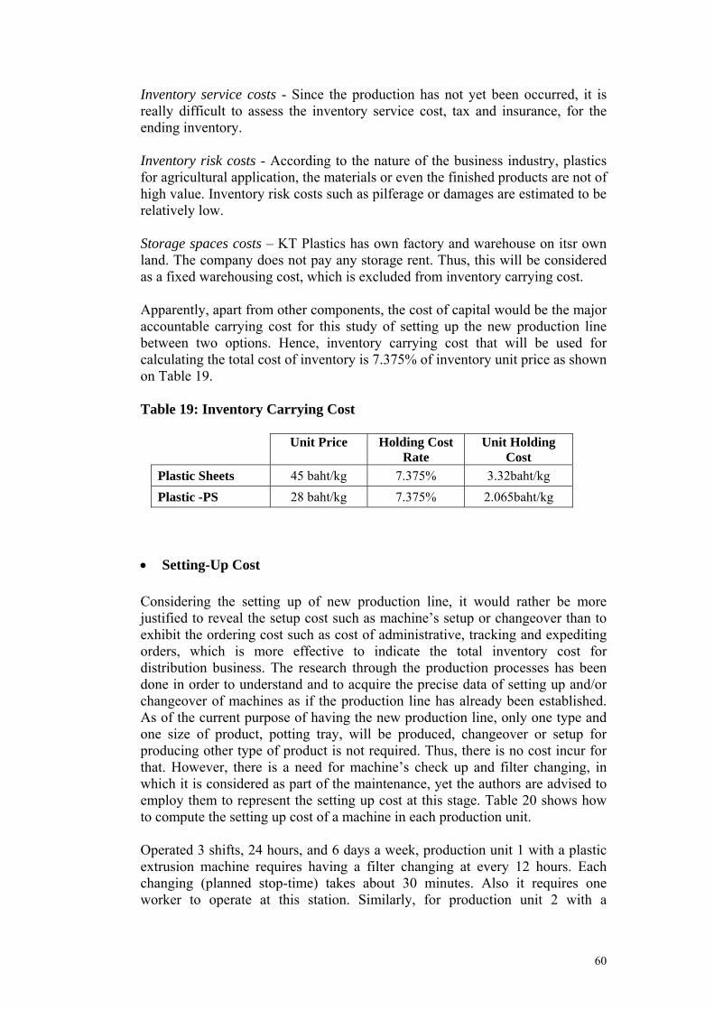
Inventory service costs - Since the production has not yet been occurred, it is really difficult to assess the inventory service cost, tax and insurance, for the ending inventory. Inventory risk costs - According to the nature of the business industry, plastics for agricultural application, the materials or even the finished products are not of high value. Inventory risk costs such as pilferage or damages are estimated to be relatively low. Storage spaces costs – KT Plastics has own factory and warehouse on itsr own land. The company does not pay any storage rent. Thus, this will be considered as a fixed warehousing cost, which is excluded from inventory carrying cost. Apparently, apart from other components, the cost of capital would be the major accountable carrying cost for this study of setting up the new production line between two options. Hence, inventory carrying cost that will be used for calculating the total cost of inventory is 7.375% of inventory unit price as shown on Table 19. Table 19: Inventory Carrying Cost

Unit Price Holding Cost

Rate Unit Holding

Cost

Plastic Sheets 45 baht/kg 7.375% 3.32baht/kg Plastic -PS 28 baht/kg 7.375% 2.065baht/kg

• Setting-Up Cost

Considering the setting up of new production line, it would rather be more justified to reveal the setup cost such as machine’s setup or changeover than to exhibit the ordering cost such as cost of administrative, tracking and expediting orders, which is more effective to indicate the total inventory cost for distribution business. The research through the production processes has been done in order to understand and to acquire the precise data of setting up and/or changeover of machines as if the production line has already been established. As of the current purpose of having the new production line, only one type and one size of product, potting tray, will be produced, changeover or setup for producing other type of product is not required. Thus, there is no cost incur for that. However, there is a need for machine’s check up and filter changing, in which it is considered as part of the maintenance, yet the authors are advised to employ them to represent the setting up cost at this stage. Table 20 shows how to compute the setting up cost of a machine in each production unit. Operated 3 shifts, 24 hours, and 6 days a week, production unit 1 with a plastic extrusion machine requires having a filter changing at every 12 hours. Each changing (planned stop-time) takes about 30 minutes. Also it requires one worker to operate at this station. Similarly, for production unit 2 with a

60

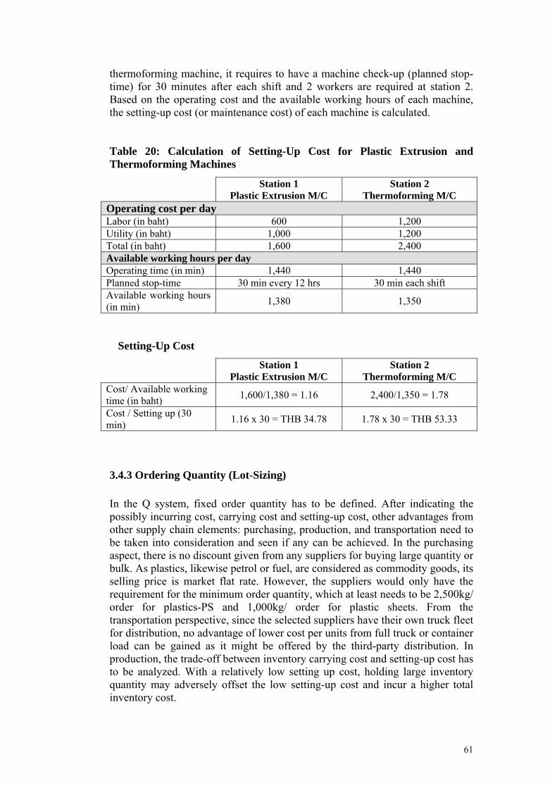
thermoforming machine, it requires to have a machine check-up (planned stop-time) for 30 minutes after each shift and 2 workers are required at station 2. Based on the operating cost and the available working hours of each machine, the setting-up cost (or maintenance cost) of each machine is calculated. Table 20: Calculation of Setting-Up Cost for Plastic Extrusion and Thermoforming Machines

Station 1 Station 2 Plastic Extrusion M/C Thermoforming M/C Operating cost per day Labor (in baht) 600 1,200 Utility (in baht) 1,000 1,200 Total (in baht) 1,600 2,400 Available working hours per day Operating time (in min) 1,440 1,440 Planned stop-time 30 min every 12 hrs 30 min each shift Available working hours (in min) 1,380 1,350

Setting-Up Cost

Station 1 Station 2

3.4.3 Ordering Quantity (Lot-Sizing)

In the Q system, fixed order quantity has to be defined. After indicating the possibly incurring cost, carrying cost and setting-up cost, other advantages from other supply chain elements: purchasing, production, and transportation need to be taken into consideration and seen if any can be achieved. In the purchasing aspect, there is no discount given from any suppliers for buying large quantity or bulk. As plastics, likewise petrol or fuel, are considered as commodity goods, its selling price is market flat rate. However, the suppliers would only have the requirement for the minimum order quantity, which at least needs to be 2,500kg/ order for plastics-PS and 1,000kg/ order for plastic sheets. From the transportation perspective, since the selected suppliers have their own truck fleet for distribution, no advantage of lower cost per units from full truck or container load can be gained as it might be offered by the third-party distribution. In production, the trade-off between inventory carrying cost and setting-up cost has to be analyzed. With a relatively low setting up cost, holding large inventory quantity may adversely offset the low setting-up cost and incur a higher total inventory cost.

Plastic Extrusion M/C Thermoforming M/C Cost/ Available working time (in baht) 1,600/1,380 = 1.16 2,400/1,350 = 1.78

Cost / Setting up (30 min) 1.16 x 30 = THB 34.78 1.78 x 30 = THB 53.33

61

After considering the inventory holding cost against other supply chain trade-offs, there is no incentive for ordering a big lot-size or no advantage can be gained from any specific ordering quantity for these materials. Hence, it is suggested to find economic order quantity (EOQ) or economic production lot size (ELS) to employ as a benchmark when making orders or productions and to minimize the overall inventory cost, balancing carrying cost and setting-up. Based on 2008 annual demand, the below illustration of EOQ and ELS calculations are shown for option 1 and 2 respectively. The graph, plotted with several lot-size alternatives, is used to display how inventory holding cost, setting up cost, and total cost curve function. Moreover, the graph exhibits the impact of safety stock to the total annual inventory cost function. Option 1: Partly outsource Only station 2 - Thermoforming machine

Raw material – Plastic sheet rolls Annual Demand (D) = 65,880 kg

Carrying Cost (C ) = 3.32baht/kg h Setting up Cost (C ) = 53.33 baht o

= = 1,454.82 ≈ 1,455 kg

2 D Co

Ch

EOQ =

3.32

2(65,880)(53.33)

(Q/2) + C (D/Q) Total annual cost = Ch o Parameters

Minimum order quantity Lot Size (Q)

Economic Order Quantity 1,455 kg1,000 kg Demand (D) 65,880 kg Setting-up Cost (C

Annual Costs Annual Cost based on EOQ

o) 53.33 THBUnit Holding Cost (C 3.32 THB h)

65.88Setup per Year Setup per Year 45.28Annual Setting-up Cost 3,513.38 THB Annual Setting-up Cost 2,414.70 THBAnnual Holding Cost 1,660 THB Annual Holding Cost 2,415.30 THBAnnual Inventory Cost 5,173.38 THB Annual Inventory Cost 4,830 THB

62

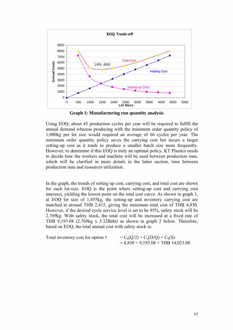
EOQ Trade-off

Holding Cost

Setting-up Cost

1455, 4830Total Cost

0

1000

2000

3000

4000

5000

6000

7000

8000

9000

0 500 1000 1500 2000 2500 3000 3500 4000 4500 5000Lot Sizes

Ann

ual C

osts

Graph 1: Manufacturing run quantity analysis

Using EOQ, about 45 production cycles per year will be required to fulfill the annual demand whereas producing with the minimum order quantity policy of 1,000kg per lot size would required an average of 66 cycles per year. The minimum order quantity policy saves the carrying cost but incurs a larger setting-up cost as it tends to produce a smaller batch size more frequently. However, to determine if this EOQ is truly an optimal policy, KT Plastics needs to decide how the workers and machine will be used between production runs, which will be clarified in more details in the latter section, time between production runs and resources utilization. In the graph, the trends of setting up cost, carrying cost, and total cost are shown for each lot-size. EOQ is the point where setting-up cost and carrying cost intersect, yielding the lowest point on the total cost curve. As shown in graph 1, at EOQ lot size of 1,455kg, the setting-up and inventory carrying cost are matched at around THB 2,415, giving the minimum total cost of THB 4,830. However, if the desired cycle service level is set to be 95%, safety stock will be 2,769kg. With safety stock, the total cost will be increased at a fixed rate of THB 9,193.08 (2,769kg x 3.32Baht) as shown in graph 2 below. Therefore, based on EOQ, the total annual cost with safety stock is: Total inventory cost for option 1 = C (Q/2) + C (D/Q) + C (S) h o h = 4,830 + 9,193.08 = THB 14,023.08

63

EOQ Trade-off

Holding Cost

Setting-up Cost

1455, 14023.08 Total Cost

02000400060008000

100001200014000160001800020000

0 500 1000 1500 2000 2500 3000 3500 4000 4500 5000Lot Sizes

Ann

ual C

osts

Graph 2: Manufacturing run quantity analysis (with safety stock)

Option 2: Fully produce in-house In order to minimize the total inventory cost of the whole production line, the company is suggested to firstly find the economic production lot size (ELS) and its cost for plastic sheets needing to process in station 2, thermoforming machine, and then compute backward for the cost of plastic -PS required to produce that economic batch size of plastic sheet. After processing plastics-PS through the plastic extrusion machine, work-in-process (WIP) of plastic sheet rolls is created with approximate weight of 5% less than the original weight of plastics-PS due to processing loss. In this step, the non-instantaneous replenishment method is applied to find the ELS and to calculate for the cost of plastic sheets, WIP, inventory. Station 2 – Thermoforming machine Work-in-process (WIP) – Plastic sheet rolls Annual Demand (D) = 65,880 kg

) for plastic sheet rolls = 3.32baht/kg Carrying Cost (Ch Setting up Cost (C ) for thermoforming machine = 53.33 baht o

Production rate (p) of extrusion machine per week = 19,320kg

- Maximum capacity = 140 kg / hr - Available working hours/week = 23 hr x 6 days = 138 hours

Demand rate (d) for plastic sheets per week = 1,267 kg

=

2 D Co

ChELS =

p p - d

19,320

19,320-1,267 3.32

2(65,880)(53.33)

64

= (1,454.82) (1.034)

= 1,505 kg Total annual cost:

C = Q/2 (p-d/p) (Ch) + D/Q (C ) o Parameters

Minimum order quantity Lot Size (Q)

Economic Production Lot Size 2,375** kg 1,505 kg

Demand (D) 65,880 kg Setting-up Cost (C

Annual Costs Annual Cost based on EOQ

**Minimum order quantity, lot-size (Q) for plastic -PS

= 2,500kg x 95% = 2,375 kg of plastic sheets created after processing thru extrusion machine

ELS Trade-off

Holding Cost

Setting-up Cost

Total Cost1505, 4668.93

0

1000

2000

3000

4000

5000

6000

7000

8000

9000

0 500 1000 1500 2000 2500 3000 3500 4000 4500 5000Lot Sizes

Ann

ual C

osts

Graph 3: Production lot-size analysis for plastic sheet (WIP)

As shown in graph 3, the optimal production lot size for plastic sheet is 1,505kg and it will give the lowest cost for the WIP inventory of THB 4,668.93. Nevertheless, as the total inventory cost for this whole production line is needed to be sought out, the inventory cost of acquiring raw materials, plastic -PS, has to be specified. Initially, the quantity of plastic-PS required to produce 1,505kg (ELS) of plastic sheets is needed to be calculated. Subsequently, the lot-size

o) 53.33 THBUnit Holding Cost (C 3.32 THBh)

69.35Setup per Year Setup per Year 43.77Annual Setting-up Cost 1,479.32 THB Annual Setting-up Cost 2,334.47 THBAnnual Holding Cost 3,683.95 THB Annual Holding Cost 2,334.46 THBAnnual Inventory Cost 5,163.27 THB Annual Inventory Cost 4,668.93 THB

65

quantity of plastic -PS is applied to compute for the inventory cost of raw materials. Finally, the inventory cost incurred from having both station 1 and 2 are summed up, yielding the total cost of inventory for option 2. As stated in the production ratio, the weight of plastic sheet output will be approximately 5% less than the weight of plastic -PS input due to the loss during processing. Thus, if the output of plastic sheet is required to be 1,505kg, approximately the input of plastic -PS should be 1,584.21 ≈ 1,585kg. However, as the order quantity for plastic-PS is required to be at least 2,500kg per order, the company has to place order based on this requirement, though having the EOQ/ELS would give the optimal inventory cost. Station 1- Plastic extrusion machine

Raw material- Plastic -PS Annual Demand (D) = 69,347 kg

Quantity, lot-size (Q) = 2,500kg (minimum order quantity) Safety Stock at 95% cycle-service level = 2,857 kg Carrying Cost (C ) = 2.065 baht/kg h Setting up Cost (C ) = 34.78 baht o Total annual cost = C (Q/2) + C (D/Q) + C (S) h o h

= 2.065 (2,500/2) + 34.78 (69,347/2,500) + 2.065 (2,857) = 2,581.25 + 964.76 + 5,899.71 = THB 9,445.72

Total inventory cost for option 2 = Cost of station 1 + Cost of station 2

= 9,445.72 + 5,163.27 = THB 14,608.99

Based on 2008-2012 forecasted demand, total annual inventory cost for option 1 and 2 are summarized below.

OPTION 1: Raw material: plastic sheet rolls Holding cost (Ch) = 3.32 baht/kg Setting up cost (Co) = 53.33 Baht Total annual cost = C (Q/2) + C (D/Q) + C (S) h o h

Station 2 2008 2009 2010 2011 2012 65,880 90,320 116,880 143,440 170,000 Annual Demand (D) 1,455 1,703 1,938 2,147 2,337 Economic lot size (EOQ) 1,000 1,000 1,000 1,000 1,000 Minimum order quantity 2,769 3,846 5,099 5,779 8,741 Safety Stock (S)

2,415.00 2,827.69 3,216.70 3,563.49 3,879.40 Annual holding cost: Ch(Q/2) 2,415.00 2,827.69 3,216.70 3,563.49 3,879.40 Annual setup cost: Co(D/Q) 9,193.08 12,768.72 16,928.68 19,186.28 29,020.12 Safety stock cost: Ch(S) 14,023.08 18,424.10 23,362.08 26,313.26 36,778.92 Total annual inventory cost

66

Option 1 total inventory cost for 5 years: THB 118,901.44

OPTION 2: Work-in-process: plastic sheet rolls Holding cost (Ch) = 3.32 baht/kg Setting up cost (Co) = 53.33 Baht Cost = Q/2 (p-d/p) (Ch) + D/Q (C ) o

Station 2 2008 2009 2010 2011 2012 Annual demand (D) 65,880 90,320 116,880 143,440 170,000 Production rate/wk: Extrusion 19,320 19,320 19,320 19,320 19,320 m/c (p) Avg weekly demand (d) 1,267 1,669 2,248 2,758 3,269 Economic production runs (ELS) 1,505 1,782 2,061 2,319 2,564 WIP Quantity* 2,375 2,375 2,375 2,375 2,564 Annual holding cost: Ch(Q/2)[(p- 3,683.95 3,601.86 3,483.83 3,379.60 3,535.97 d)/p] Annual setting up cost: Co(D/Q) 1,479.32 2,028.11 2,624.51 3,220.91 3,535.97 Total annual inventory cost 5,163.27 5,629.97 6,108.34 6,600.51 7,071.94

*Created after the minimum order quantity requirement of Plastic-PS (2,500kg) has been processed thru extrusion machine

Raw material: plastic -PS Holding cost (Ch) = 2.065 baht/kg Setting up cost (Co) = 34.78 Baht Annual cost = C (Q/2) + C (D/Q) + C (S) h o h

Station 1 2008 2009 2010 2011 2012 Annual Demand (D) 69,347 95,074 123,032 150,989 178,947 Quantity required to produce 1,585 1,876 2,170 2,441 2,699 ELS for plastic sheets** Minimum order quantity 2,500 2,500 2,500 2,500 2,500 Quantity, lot-size (Q) 2,500 2,500 2,500 2,500 2,699 Safety Stock 2,857 4,080 5,049 5,557 8,511 Annual holding cost [Ch(Q/2)] 2,581.25 2,581.25 2,581.25 2,581.25 2,786.62 Annual setting up cost [Co(D/Q)] 964.76 1,322.67 1,711.62 2,100.57 2,306.04 Safety stock cost [Ch(S)] 5,899.71 8,425.2 10,426.2 11,475.21 17,575.215Total annual inventory cost 9,445.72 12,329.12 14,719.05 16,157.02 22,667.88

** Weight of plastic-PS is approximately 5% more than plastic sheet (ELS)

Station 1 & 2 2008 2009 2010 2011 2012 Total annual inventory cost 14,608.99 17,959.09 20,827.39 22,757.53 29.739.82

Option 2 total inventory cost for 5 years: THB 105,892.84

67

The reason why option 1 incurs higher total inventory cost than option 2 is mainly because of the cost of safety stock. There are two factors that cause safety stock cost for option 1 to be rather high. Firstly, the average distribution lead time for the supply of plastic sheet rolls is longer than that of the supply of plastics-PS, 3.45 days to 2.75 days. Secondly with the same rate of opportunity cost, 7.375%, plastic sheet rolls with a higher value of 45 baht/kg incur a higher holding cost of 3.32 baht/kg than the plastics-PS, which cost only 28 baht/kg and incur a holding cost of 2.065 baht/kg. As option 1 holds plastic sheet rolls as raw material to be used in processing, it tends to hold an adequate amount of safety stock to buffer against demand fluctuation due to longer delivery lead time of plastic sheet rolls. Comparing to option 2, which has plastics-PS as raw material with shorter time to supply and lower holding cost per unit, a higher level of safety stock and a higher holding cost of plastic sheet rolls lead to an incremental fixed cost for option 1.

3.4.4 Time between Production Runs (TBP) and Resources Utilization

The time between production runs (TBP) has been computed so as to give the average elapsed/cycle time in a year that the production is needed to operate in order to fulfill each annual forecasted demand by the particular efficient lot sizes. After the average elapsed time has been specified, given the production rate of each station, the time required to process these efficient lot sizes will be calculated and put as the ratio to the average elapsed time. Indicating the utilization rate, these figures will be employed to measure the degree to which the machine and workforce are being utilized. Since the utilization rate points out the need for adding capacity or eliminating unneeded capacity, it is another factor used to support in decision making. Based on 2008 forecasted demand and EOQ/ ELS, the time between production runs for both options 1 and 2 will be computed as well as the time each station required to process an efficient lot size. Accordingly, the utilization percentage of each station is derived from the ratio of the processing time of an efficient lot size (average time based on a machine’s production rate) to the time between production runs (maximum time required to satisfy the demand).

Time between Production Runs (TBP) Option 1: Station 2 TBP = EOQ/D = 1,455/ 65,880 = 0.0221 year EOQ = EOQ/D (300 working days/year) = 1,455/ 65,880 (300)

= 6.6 ≈ 6 working days

68

Option 2: Station 1 TBP = Lot-size/D = 2,500/69,347 = 0.036 year PS = Lot-size/D (300 working days/year) = 2,500/69,347 (300) = 10.8 ≈ 11 working days Station 2 TBP = WIP/D = 2,375/ 65,880 = 0.036 year WIP = WIP /D (300 working days/year) = 2,375/ 65,880 (300) = 10.8 ≈ 11 working days In option 1, using EOQ, a production at station 2 requires to operate approximately every 6 working days in order to fulfill the 2008 annual demand whereas, in option 2, applying plastic-PS minimum order lot-size of 2,500kg (≈2,375kg of plastic sheets-WIP), about every 11 working days that the production at both station 1 and 2 is required to fulfill the 2008 annual demand Production rate of machine at each station Station 1 – Plastic extrusion machine.

1Production rate/ day = maximum capacity/hour x available working hr/day = 140 kg/hr x 23 hr/day = 3,220 kg/day Station 2 – Thermoforming machine

2Production rate/ day = maximum capacity/hour x available working hr/day = 19.10 kg/hr x 22.5 hr/day = 429.75 kg/day The Utilization of Each Production Unit Option 1: Station 2 - Thermoforming machine Time required to process EOQ = EOQ / production rate per day = 1455 / 429.75 = 3.4 ≈ 3 working days. Producing at the production rate of 429.75kg per day, production unit 2 can process EOQ of 1,455 kg within approximately three working days. Given the time between production runs of approximately six working days, this means there will be roughly three working days before another production runs starts. Thus, the utilization rate of station 2 in option 1 is:

1 See the machine specification from Appendix 2 See the machine specification in Appendix

69

Utilization rate = Time required to process EOQ / Time between production runs = 3.4 days / 6.6 days = 0.51099 x 100% = 51.10% Option 2: Station 1 – Plastic extrusion machine. Time required to process Lot-size = Lot-size / production rate per day = 2,500 / 3220 = 0.78 ≈ 0.8 working days. Utilization rate = Time required to process lot-size / Time between production runs = 0.8 days / 10.8 days = 0.07179 x 100% = 7.18% Station 2 - Thermoforming machine Time required to process WIP = WIP / production rate per day = 2,375 / 429.75 = 5.5 working days. Utilization rate = Time required to process WIP / Time between production runs = 5.5 days / 10.8 days = 0.51099 x 100% = 51.10% Station 1 and station 2 have the production rate of 3,220 kg and 429.75 kg per day respectively. In each production cycle, station 1, with the input of plastics-PS lot size of 2,500kg (minimum order requirement), requires only about 0.8 working days to operate and creates the plastic sheet output (WIP) of 2,375 kg, while station 2 can process WIP of 2,375 kg within 5.5 working days. Given the time between production runs of 11 working days, only about 7% and 51% of resources at station 1 and 2 are utilized respectively. Based on five years forecast of annual demand (2008-2012), the utilization rate of each station in option 1 and 2 are shown on the tables below. Option 1: Station 2 – Thermoforming machine

2008 2009 2010 2011 2012 Annual Demand (D) 65,880 90,320 116,880 143,440 170,000 Economic lot size (EOQ) 1,455 1,703 1,938 2,147 2,337 Time b/w production runs-TBP (in day) 6.625 5.658 4.974 4.490 4.124 Production rate/ day (in kg) 429.75 429.75 429.75 429.75 429.75 Time required to process EOQ (in day) 3.385 3.964 4.509 4.995 5.438 Utilization rate (%) 51.10% 70.06% 90.66% 111.26% 131.86%

70

Option 2: Station 1 – Plastic extrusion machine

2008 2009 2010 2011 2012 Annual Demand (D) 69,347 95,074 123,032 150,989 178,947 Quantity, lot-size (Q) 2500 2500 2500 2500 2699 Time b/w production runs-TBP (in day) 10.815 7.889 6.096 4.967 4.525 Production rate/ day (in kg) 3,220 3,220 3,220 3,220 3,220 Time required to process EOQ (in day) 0.776 0.776 0.776 0.776 0.838 Utilization rate (%) 7.18% 9.84% 12.74% 15.63% 18.52%

Station 2 – Thermoforming machine 2008 2009 2010 2011 2012

Annual Demand (D) 65,880 90,320 116,880 143,440 170,000 Economic production runs (ELS) 2375 2375 2375 2375 2564 Time b/w production runs-TBP (in day) 10.815 7.889 6.096 4.967 4.525 Production rate/ day (in kg) 429.75 429.75 429.75 429.75 429.75 Time required to process EOQ (in day) 5.526 5.526 5.526 5.526 5.966 Utilization rate (%) 51.10% 70.06% 90.66% 111.26% 131.86%

As per the utilization rate of the final production unit in both options, station 2-thermoforming machine shows similar result and thus assume to generate the same amount of throughput. Comparing the utilization rate of station 1 and 2 in option 2, thermoforming machine in station 2 is considered as a constraint or bottleneck of the process. Although, in option 2, a plastic extrusion machine with greater production capacity has been added to the production line, the throughput for option 2 would be limited to the capacity of a constraint resource, thermoforming machine, and is equal to option 1. Therefore, if the process is limited by machine capacity (bottleneck), work will pile up in front of the limiting steps of the process, thus the throughput of this entire process is determined by the production capacity of the bottleneck (Kaydos, 1999). From this limited capacity of constraint, KT Plastics needs to question if having station 1-plastic extrusion machine is necessary and would add value to this production process right from the first year (2008). Given the study timeframe of five years, the utilization rates show that the extrusion machine is underutilized and have too high capacity cushion. The machine is not operated efficiently and may not be worth in investment to fulfill these demand levels. Capacity cushion is the amount of reserve capacity a process uses to handle sudden increases in demand or temporary losses of production capacity, measuring by which the average utilization falls below 100 percent (Krajewski, Ritzman, Malhotra, 2007). During 2008-2012, the highest utilization rate of plastic extrusion machine is only 18.52% which means it would have a capacity cushion of more than 80% (100%-18.52%) throughout these five years. For a capital-intensive firm with high investment in machines or equipments, like KT Plastics, having a small capacity cushion is rather preferable as unused capacity costs money. However, to determine if investing in station 1 would be worthwhile, one thing that KT Plastics needs to concern about is how to employ

71

the workers and machine efficiently between production runs as the size of capacity cushion of station 1 is so large. As mentioned in the theory of constraint, developed by Eli Goldratt, the process should not focus only on the efficiency of individual processes, but also on the bottlenecks that constrain the system as a whole. Hence, it is suggested that the flows of bottleneck should be equal to the market demand so as to minimize the inventory and operating expenses. Based on five years forecasted demand, the utilization rate of station 2 shows that the capacity of thermoforming machine is underutilized until the third year (2010), where the appropriate size of capacity cushion (about 10%) is maintained. It is advised that the average utilization rates for any resource should not get too close to 100 percent over the long term. However, in the last two year of forecasted demand, 2011-2012, thermoforming machine’s utilization percentage proves that the machine capacity is exceeded, KT Plastics may need to consider of having capacity expansion after year three (2010), either by short-term option such as use of subcontractors or long-term expansion such as buying additional thermoforming machine and perhaps acquiring a plastic extrusion machine by that time. Yet, to decide between two options, the other quantitative, decision making models and techniques involving financial perspective will be explored in the next section and employed to suggest a more accurate conclusion.

72

Chapter 4: Analysis and Result

4.1 Quantitative Analysis: Decision-Making Techniques As discussed in the preceding section, the qualitative concerns for these alternatives have been assessed. In this part, different decision making techniques, quantitative approaches, will be exploited to evaluate between the two alternatives. Also the cash flow for each alternative over the forecast time horizon will be compared and evaluated. In this study, break-even analysis and decision tree are the chosen techniques used to analyze and to confirm the decision making. Obviously, there are the criteria that affect the choice of technique. As the figure of the utilization rate of each station evidently showed and analyzed in the “Time between Production Runs (TBP) and Resources Utilization” section, break even analysis is chosen to verify the make or buy decision, whether to make the plastic sheets in-house or to buy from supplier. Taking the financial aspect (cost of two alternatives) into consideration, the break-even point is derived where the sales volume of potting tray above and below that point is going to be profitable to the make and buy decision respectively. Through break-even analysis, the decision can be made more confidently as the profitable level of estimated sales is quantified. One of the advantages of the break-even analysis is that they are easy to understand, especially when presented graphically. (Ballot, 1986) Since the scope of decision has to be made under a condition of risk where the set of future events and the probability of occurrence can be identified, decision tree method is selected as another tool to analyze and corroborate the decision making. As the production line has not yet been in place, there exist a set of alternatives or future events that need to be evaluate and each could yield different results for different environment. Using decision tree, the alternative-event combination with the best expected value (pay-offs) is chosen.

4.1.1 Break-Even Analysis: Make or Buy

Generally, break-even analysis is used to determine the volume of sales at which the product or service breaks even, or in other words, to find the quantity at which total revenues equal total costs. The break-even quantity is exploited as a guideline to determine if the predicted sales volume of the product would either earn a profit (forecasted sales volume > break-even point) or sustain a loss (forecasted sales volume < break-even point). However, when a choice has to be made between two processes or between an internal process and buying materials from the outside, break even analysis can also be useful to compare the processes. In this case, the decision does not affect revenues, yet the cost of the two approaches is compared. Thus, all the cost and advantages of each alternative needs to be studied and identified. To find out the break-even quantity for the make or buy analysis, the equation is set for which the total cost

73

functions of the two alternatives are equal. One side represents the cost of buying plastic sheets from a supplier whereas the other side represents the cost of making them in-house, based on the assumption that all costs related to the production can be divided into two categories: variable costs3 4 and fixed costs

F + c Q = Fb b m + cmQ where: F = fixed cost per year of the buy option b Fm = fixed cost of the make option cb = variable cost per unit of the buy option cm = variable cost of the make option Q = break-even quantity Solve for break-even quantity (Q):

Fm - Fb

cb - cm Q =

Fixed Costs (F) per year (THB)

Variable costs (c) per kg (THB)

Thermoforming machine* 0.41M Labor** 0.36M Utilities 0.36M

Buy Option

Plastic sheets 45 Plastic extrusion machine* 0.7M Thermoforming machine* 0.41M Labor** 0.54M Utilities 0.66M

Make Option

Plastic 28 * Thermoforming machine costs 2.05M and plastic extrusion machine costs 3.5M (divided by five to yield the annual cost for the time study). ** Wages are paid daily despite of the level of production.

2.31M – 1.13M

45 - 28

Q =

1.18M17

Q =

Q = 69,411.7 ≈ 69,412 kg

3 Cost that varies directly depends on the amount of output produced e.g. materials cost per unit or labor. 4 Cost that remains constant regardless of changes in level of production e.g. annual cost of renting or buying new equipment, salaries, and utilities, etc.

74

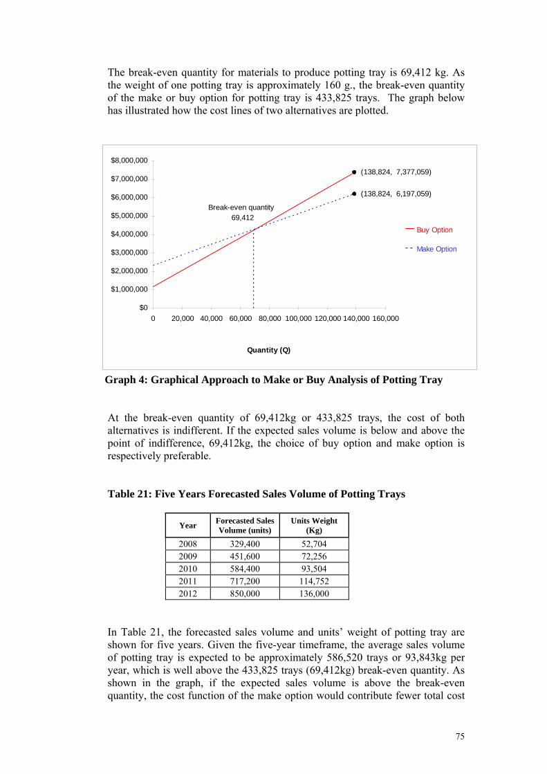
The break-even quantity for materials to produce potting tray is 69,412 kg. As the weight of one potting tray is approximately 160 g., the break-even quantity of the make or buy option for potting tray is 433,825 trays. The graph below has illustrated how the cost lines of two alternatives are plotted.

Break-even quantity 69,412

(138,824, 7,377,059)

(138,824, 6,197,059)

$0

$1,000,000

$2,000,000

$3,000,000

$4,000,000

$5,000,000

$6,000,000

$7,000,000

$8,000,000

0 20,000 40,000 60,000 80,000 100,000 120,000 140,000 160,000

Quantity (Q)

Buy Option

Make Option

Graph 4: Graphical Approach to Make or Buy Analysis of Potting Tray

At the break-even quantity of 69,412kg or 433,825 trays, the cost of both alternatives is indifferent. If the expected sales volume is below and above the point of indifference, 69,412kg, the choice of buy option and make option is respectively preferable.

Table 21: Five Years Forecasted Sales Volume of Potting Trays

Forecasted Sales Volume (units)

Units Weight (Kg) Year

2008 329,400 52,704 2009 451,600 72,256 2010 584,400 93,504 2011 717,200 114,752 2012 850,000 136,000

In Table 21, the forecasted sales volume and units’ weight of potting tray are shown for five years. Given the five-year timeframe, the average sales volume of potting tray is expected to be approximately 586,520 trays or 93,843kg per year, which is well above the 433,825 trays (69,412kg) break-even quantity. As shown in the graph, if the expected sales volume is above the break-even quantity, the cost function of the make option would contribute fewer total cost

75

than the buy option. Hence, from this analyzed method, the make option is preferred. However, this method alone is not able to finalize the decision as it does not concern the real cash flow. Later, the other two methods, cash flow and decision tree analysis, which involve the cash flow and time value of money will be discussed and analyzed shortly.

4.1.2 Cash Flow Analysis

Cash flow analysis is used to evaluate the project alternatives’ cash flow, the difference between the flow of funds into and out of the firm over a period of time including revenues, cost, and changes in assets and liabilities (Krajewski, Ritzman, Malhotra, 2007). The base case for establishing potting tray production line is to acquire only thermoforming machine and buy plastic sheets from supplier at 45 baht/kg. The capacity alternatives for this production line are two-stage expansion. The capacity of thermoforming machine in the base case is approximately 644,625 trays (103,140 kg) per year. Based on five years forecasted sales, the capacity of thermoforming machine will not be sufficient to fulfill the 2011 demand, therefore one alternative is to acquire another thermoforming machine at the end of year three (2010). Another two alternatives concern the investment in plastics extrusion machine, either to acquire it right from the first year 2008 or at the same time buying thermoforming machine at the end of 2010. For the last two alternatives, according to theory of constraints, buying plastic extrusion machine does not increase throughput of the production line as the bottleneck which determine the throughput is at thermoforming machine. However, if KT Plastics acquire plastic extrusion machine, raw materials requires to process in the machine should be plastic, which costs 28 baht/kg., instead of plastic sheets. Since the cash flow analysis involve revenue and cost, lower cost of raw material (variable cost) would affect the pretax profit, thus impact to the cash flow for these alternatives. Average selling price of potting tray is 14 baht per tray and the tax rate is 15%. For comparison purposes the NPV of these alternatives at a discount rate of 8% (average cost of capital) is calculated.

76

Base case: an initial investment in thermoforming machine is THB 2.05M at the end of year 0 with the pretax profit of THB 3.10/unit all through five years. Potential sales beyond 644,625 trays will be loss due to the capacity of a thermoforming machine.

Projected Demand

(units/year)

Projected Capacity

(units/year)

Cash Inflow (Outflow) Year Calculation of After-tax Profit

in Baht

0 - 644,625 Initial investment in thermoforming machine (2,050,000)

1 329,400 644,625 (329,400 units) (THB 2.64/unit) 869,616

2 451,600 644,625 (451,600 units) (THB 2.64/unit) 1,192,224

3 584,400 644,625 (584,400 units) (THB 2.64/unit) 1,542,816

4 717,200 644,625 (644,625 units) (THB 2.64/unit) 1,701,810

5 850,000 644,625 (644,625 units) (THB 2.64/unit) 1,701,810

NPV = -2,050,000 + (869,616/1.08) + [1,192,224/(1.08)2] + [1,542,816/(1.08)3] +

[1,701,810/(1.08)4] + [1,701,810/(1.08)5] = -2,050,000 + 805,200 + 1,022,094 + 1,224,687 + 1,250,830 + 1,158,252

= THB 3,411,063

1st Alternative: an initial investment in thermoforming machine would be THB 2.05M at the end of year 0 and additional investment of 2.05M at the end of year 3. Pretax profit of year 1-3 is THB 3.10/unit while year 4-5 is THB 3.38/unit.

Projected Demand

(units/year)

Projected Capacity

(units/year)

Cash Inflow (Outflow) Year Calculation of After-tax Profit

in Baht

0 - 644,625 Initial investment in thermoforming machine (2,050,000)

1 329,400 644,625 (329,400 units) (THB 2.64/unit) 869,616

2 451,600 644,625 (451,600 units) (THB 2.64/unit) 1,192,224

3 584,400 644,625 (584,400 units) (THB 2.64/unit) 1,542,816

Add another thermoforming machine, increasing total capacity to 1,289,250 trays (2,050,000)

(507,184)

4 717,200 1,289,250 (717,200 units) (THB 2.87/unit) 2,058,364

5 850,000 1,289,250 (850,000 units) (THB 2.87/unit) 2,439,500

NPV = -2,050,000 + (869,616/1.08) + [1,192,224/(1.08)2] - [507,184/(1.08)3] +

[2,058,364/(1.08)4] + [2,439,500/(1.08)5] = -2,050,000 + 805,200 + 1,022,094 - 402,603 + 1,512,898 + 1,660,324 = THB 2,547,913

77

2nd Alternative: With an initial investment in thermoforming machine of THB 2.05M at the end of year 0, it requires to make an additional investment of THB 5.55M in thermoforming machine and plastic extrusion machine at the end of year 3. THB 3.10/unit and THB 5.57/unit goes to pretax profit in year 1-3 and year 4-5 respectively.

Projected Demand

(units/year)

Projected Capacity

(units/year)

Cash Inflow (Outflow) Year Calculation of After-tax Profit

in Baht

0 - 644,625 Initial investment in thermoforming machine (2,050,000)

1 329,400 644,625 (329,400 units) (THB 2.64/unit) 869,616

2 451,600 644,625 (451,600 units) (THB 2.64/unit) 1,192,224

3 584,400 644,625 (584,400 units) (THB 2.64/unit) 1,542,816

Add another thermoforming machine and a plastic extrusion machine, increasing total capacity to 1,289,250 trays

(5,550,000)

(4,007,184)

4 717,200 1,289,250 (717,200 units) (THB 4.73/unit) 3,392,356

5 850,000 1,289,250 (850,000 units) (THB 4.73/unit) 4,020,500

NPV = -2,050,000 + (869,616/1.08) + [1,192,224/(1.08)2] - [4,007,184/(1.08)3] +

[3,392,356/(1.08)4] + [4,020,500/(1.08)5] = -2,050,000 + 805,200 + 1,022,094 – 3,180,903 + 2,493,382 + 2,758,063 = THB 1,847,836

3rd Alternative: the initial investment of THB 5.55M has to be made for thermoforming machine and plastic extrusion machine at the end of year 0 with the pretax profit of THB 4.38/unit in year 1-3 and additional investment of THB 2.05M in thermoforming machine at the end of year 3 with the pretax profit of THB 5.57/unit in year 4-5.

Projected Demand

(units/year)

Projected Capacity

(units/year)

Cash Inflow (Outflow) Year Calculation of After-tax Profit

in Baht

0 - 644,625 Initial investment in thermoforming and plastic extrusion machine (5,550,000)

1 329,400 644,625 (329,400 units) (THB 3.72/unit) 1,225,368

2 451,600 644,625 (451,600 units) (THB 3.72/unit) 1,679,952

3 584,400 644,625 (584,400 units) (THB 3.72/unit) 2,173,968

Add another thermoforming machine, increasing total capacity to 1,289,250 trays (2,050,000)

123,968

4 717,200 1,289,250 (717,200 units) (THB 4.73/unit) 3,392,356

5 850,000 1,289,250 (850,000 units) (THB 4.73/unit) 4,020,500

NPV = -5,550,000 + (1,225,368/1.08) + [1,679,952/(1.08)2] + [123,968/(1.08)3] +

[3,392,356/(1.08)4] + [4,020,500/(1.08)5] = -5,550,000 + 1,134,600 + 1,440,223 + 98,406 + 2,493,382 + 2,758,063 = THB 2,374,674

78

On a purely monetary basis, base case seems to offer the highest cash inflow (THB 3.41M) among all these alternatives. In the 1st alternative, gaining quantity of demand in year 4 and 5 that exceeds the capacity of one thermoforming machine is not sufficient to cover the additional investment for another thermoforming machine at the end of year 3, thus yield lower cash inflow (THB 2.55M) than base case. For 2nd rd and 3 alternatives, though lower cost of raw materials contribute to a higher profit per unit, an additional investment has to be made for a relatively costly plastic extrusion machine, which do not at all affect the number of throughput or the efficiency of this production line in this scenario. Therefore, the cash inflow (THB 1.85M and THB 2.37M) of the last two alternatives (with plastic extrusion machine investment) yields a lower cash flow than base case and the 1st alternative. Nevertheless, the net present value of all these alternatives is positive to the discount rate used. Choosing either of these alternatives, the investment still earns a rate of return higher than the discount rate. Considering other qualitative factor, however, the management might see one alternative better than the base case.

4.1.3 Decision Tree Analysis

Decision tree is a very useful tool and particularly valuable for analyzing a set of alternatives when demand or environments in the future is uncertain and sequential decisions are involved (Ballot, 1986). In the decision tree model, the available alternatives along with their possible consequences are shown. A circular node represents different events for an alternative, which associated with probabilities of chance that those events might occur. The probability of all chance events must sum to 1.0. At the end points, it shows expected payoff for each possible alternative-event combination. Solving from right to left, multiply each payoff’s event by the event’s probability and add these products to get the event node’s expected payoff. When it comes to the square nodes, representing the decision point, the alternative with the best expected payoff event node is chosen. The process is continued until the leftmost decision node is reached.

79

Decision Tree Model

1st decision

Alternative 1

Alternative 2

E1 [P(E1)]

E2 [P(E2)]

E3[P(E3)]

E1 [P(E1)]

E2 [P(E2)]

E3[P(E3)]

Alternative 1

Alternative 2

Alternative 3 Possible 2nd decision

Payoff 1

Payoff 2

Payoff 3

Payoff 4

Payoff 5

Payoff 6

Payoff 7

Payoff 8

= Event node

= Decision node

Ei = Event i P(Ei) = Probability of event i

According to the problem statement, KT Plastics has to make decision between the two alternatives; starting the new production line of potting tray with one machine, thermoforming machine and outsource plastic sheets from supplier or with two machines, plastic extrusion machine and thermoforming machine– make all processes in-house. In the cash flow analysis, the alternatives are analyzed regardless of other possible events that may occur in the future. However, in reality, the demand of potting tray might not happen as it is forecasted. It can be higher or lower than forecast and there might be other occurrences associated with the alternative. In this scenario, the probability of chance that demand would be higher and lower than forecast is anticipated to be 0.1 and 0.3 respectively, whereas the probability that demand is occurred as the forecasting figures would be 0.6 and is considered as moderate. Table below shows the amount of five-year demands and revenues that is lower and higher than the forecast and as per forecast.

Probability of Demand Level

* Selling price @ THB 14/unit

Low (0.3) Moderate (0.6) High (0.1) Not Expand Periods (Year)

Demand Revenue* Demand Revenue* Demand Revenue* Demand Revenue*

1 2008 280,000 3,920,000 330,000 4,620,000 380,000 5,320,000

2 2009 402,000 5,628,000 452,000 6,328,000 502,000 7,028,000

3 2010 534,000 7,476,000 584,000 8,176,000 634,000 8,876,000

4 2011 667,000 9,338,000 717,000 10,038,000 767,000 10,738,000 644,000 9,016,000

5 2012 800,000 11,200,000 850,000 11,900,000 900,000 12,600,000 644,000 9,016,000

80

In the decision tree analysis, the decision has to be made in two stages: at the beginning whether to have only thermoforming machine or to have both thermoforming machine and plastic extrusion machine, and at the end of third year whether to expand the production capacity or not. Since the production capacity of this production line is limited to the capacity of a thermoforming machine, all the demand level: high, moderate, and low in the 4th and 5th year are exceeded the production capacity. For both alternatives, if KT Plastics chooses not to expand, exceeding demand will be loss. For the first alternative, starting the production line with one machine, thermoforming machine, and outsource plastic sheets, regardless of the level of demand is high, moderate or low, KT Plastics has to choose among three alternatives at the end of third year: expand with another thermoforming machine, expand with both a thermoforming machine and a plastic extrusion machine, or not expand at all. For the second alternative, if all the production processes is to be made in-house from the beginning, KT plastic has to acquire both thermoforming machine and plastic extrusion machine. Despite of the level of demand to be high, moderate, or low, still at the end of year 3 KT Plastics have to consider if they want to expand with another thermoforming machine or not expand. However, in this second alternative, there is another event associated with having a plastic extrusion machine from the start up. As referred to the “Time between Production Runs (TBP) and Resources Utilization” section and the five-year forecasted demand, only about 20 % of the capacity of plastic extrusion machine is utilized to produce plastic sheets, which are to be processed further to produce potting tray. If plastic extrusion machine is utilized fully, there will be an excessive output of plastic sheets. In this case, KT Plastics can possibly increase their revenue by selling the excessive output of plastic sheets to other market. Selling of plastic sheets to other market may be either in a modest volume (30% of the excessive capacity) or in large volume (50% of the excessive capacity), with their probabilities estimated to be 0.5 both.

Extending market: Plastic sheets

Modest: 30% of cap (0.5) Large: 50% of cap (0.5) Sales Volume

(kg) Sales Volume

(kg) Revenue* Revenue*

280,000 12,600,000 480,000 21,600,000 * Selling price @ THB 45/kg

81

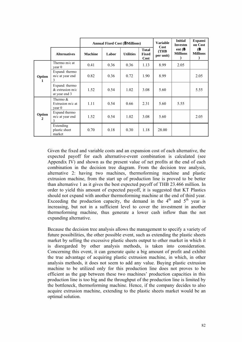
82

Given the fixed and variable costs and an expansion cost of each alternative, the expected payoff for each alternative-event combination is calculated (see Appendix IV) and shown as the present value of net profits at the end of each combination in the decision tree diagram. From the decision tree analysis, alternative 2: having two machines, thermoforming machine and plastic extrusion machine, from the start up of production line is proved to be better than alternative 1 as it gives the best expected payoff of THB 23.466 million. In order to yield this amount of expected payoff, it is suggested that KT Plastics should not expand with another thermoforming machine at the end of third year. Exceeding the production capacity, the demand in the 4th and 5th year is increasing, but not in a sufficient level to cover the investment in another thermoforming machine, thus generate a lower cash inflow than the not expanding alternative. Because the decision tree analysis allows the management to specify a variety of future possibilities, the other possible event, such as extending the plastic sheets market by selling the excessive plastic sheets output to other market in which it is disregarded by other analysis methods, is taken into consideration. Concerning this event, it can generate quite a big amount of profit and exhibit the true advantage of acquiring plastic extrusion machine, in which, in other analysis methods, it does not seem to add any value. Buying plastic extrusion machine to be utilized only for this production line does not proves to be efficient as the gap between these two machines’ production capacities in this production line is too big and the throughput of the production line is limited by the bottleneck, thermoforming machine. Hence, if the company decides to also acquire extrusion machine, extending to the plastic sheets market would be an optimal solution.

Annual Fixed Cost (฿Millions)

Alternatives Machine Labor Utilities Total Fixed Cost

Variable Cost

(THB per unit)

Initial Investment (฿

Millions)

Expansion Cost

(฿Millions

) Thermo m/c at year 0 0.41 0.36 0.36 1.13 8.99 2.05 Expand: thermo m/c at year end 3

0.82 0.36 0.72 1.90 8.99 2.05 Option 1

Expand: thermo & extrusion m/c at year end 3

1.52 0.54 1.02 3.08 5.60 5.55

Thermo & Extrusion m/c at year 0

1.11 0.54 0.66 2.31 5.60 5.55

Expand thermo m/c at year end 3

1.52 0.54 1.02 3.08 5.60 2.05 Option 2

Extending plastic sheet market

0.70 0.18 0.30 1.18 28.00

83

High (0.1)

High (0.1)

Moderate (0.6)

Low (0.3)

Low (0.3)

Do not expand

Do not expand

Do not expand

Do not expand

Do not expand

Expand: 1 m/c

Expand: 1 m/c

Expand: 1 m/c

Expand: 2 m/cs

Expand: 2 m/cs

Expand: 2 m/cs

Expand

Expand

Expand

Do nothing

Do nothing

Do nothing

Extend mkt

Extend mkt

Extend mkt

Extend mkt

Extend mkt

Extend mkt

Expand: 1 m/c

Expand: 1 m/c

Moderate (0.5)

Moderate (0.5)

Moderate (0.5)

Moderate (0.5)

Moderate (0.5)

Moderate (0.5)

Large (0.5)

Large (0.5)

Large (0.5)

Large (0.5)

Large (0.5)

Large (0.5)

THB 6.496 Million

THB 5.104

THB 4.643

THB 5.850

THB 4.104

THB 3.403

THB 5.205

THB 3.104

THB 2.163

THB 9.233THB 14.294

THB 14.294

THB 14.294

THB 14.294

THB 14.294

THB 14.294

THB 27.869

THB 27.869

THB 27.869

THB 27.869

THB 27.869

THB 27.869

THB 8.739

THB 8.151

THB 7.062

THB 7.068

THB 5.385

THB 30.315

THB 29.821

THB 29.233

THB 28.144

THB 28.15

THB 26.467

THB 21.082

THB 21.082

THB 21.082

THB 21.082

THB 21.082

THB 21.082

THB 30.315

THB 29.233

THB 28.15

THB 5.721 - 2.05 THB 3.671

THB 29.016 - 5.55 THB 23.466

Expand: 1 m/cAlternative1: One machine

Alternative2: Two machines

Moderate (0.6)

Note: Expand: 1m/c = thermoforming machine Expand: 2m/cs = thermoforming machine & plastic extrusion machine Extend mkt = selling excessive plastic sheets output to other market

Do not expand

DECISION TREE DIAGRAM

4.2 Aggregate Analysis and Result Deciding to source this production line, potting tray, back from the suppliers as to avoiding the threat from suppliers become competitors, the process done by thermoforming machine in this production line has been identified as the core process while a process at extrusion machine is considered as non-core as according to the outsourcing guideline and framework. Thereafter, the company has to decide between two options of whether to maintain only the core process in-house and outsource the non-core process (option 1) or to have the whole production line, both core and non-core process in-house (option 2). Among the qualitative and quantitative aspects, there are several facets that support the make decision (option 2). From the outsourcing questions guideline, apart from helping to identify the core process or function of the production, total cost analysis in an outsourcing framework also points out that invest to have the whole production process of this product line in-house would cost the lowest production price, thus yield the highest profit margin. Based on the five years forecasted demand, option 2 seems to have a lower total inventory cost due to the cost of raw materials (plastics-PS) is cheaper and delivery lead-time is shorter, leads to lower safety stock, comparing to option 1. From the quantitative aspect, break-even and decision tree analysis have also shown that investing in both extrusion machine and thermoforming machine would give a better benefit to the company rather than only invest in one machine, thermoforming machine. The graph analyzed in the break-even method illustrates that if the sales quantity of potting tray is above the break-even quantity, 433,825 trays, make option is preferable and vice versa. According to the forecasted sales in five years, average sales volume is 586,520 trays per year, which is well above the break-even point, thus make option is suggested in this method. In the decision tree analysis, the result shows that option 2 gives a better pay-off as there is the possibility that another event, extending to plastic sheet market, may occur. However, among all, there are two aspects that oppose the make decision. From the viewpoint of resource utilization, having extrusion machine to be utilized only in the potting trays production line is not worth in term of investment. Throughout these five years timeframe, the capacity of the extrusion machine seems to be underutilized, based on the forecasted demand level. Moreover, the cash flow analysis exhibits that investing only in one machine-thermoforming machine, as in the base case would generate the highest cash inflow to the company rather than investing in both extrusion and thermoforming machine as in 2nd and 3rd alternative. In this scenario, having extrusion machine in the production line does not seems to add any value as the number of throughput is determined by the thermoforming machine. No additional sales can be gained from the investment in extrusion machine; on the other hand, investment generates a cash outflow and thus leads to lower cash inflow for these two alternatives.

84

Chapter 5: Conclusions and Recommendations In Thailand, since high flexibility is required by both SMEs and supplier, the relationship of both parties is mostly build on trust rather than by contract. Doing business with suppliers who have no legitimated contract can further increase the risk exposure. Hence, in this circumstance, if the company wants to outsource any function, they need to pay attention in dealing with supplier, essentially identifying their core processes or functions and make sure to maintain these core processes in-house in order to avoid the problem of supplier become competitor. Outsourcing has become a strategic tool used by many organizations. The decision of whether to make or to buy the function or service, thus, can give a huge impact to the company if the decision has been made thoroughly and wisely. However, if the company does not consider it carefully and convince by only a short-term benefit, there is a high risk in losing the company’s core competency. To effectively make the outsourcing decision, both qualitative and quantitative approaches have to be taken into consideration. Business core competencies as well as the financial aspect of business decision, such as production and inventory cost, cash flow analysis, etc. need to be identified and analyze, combining with management judgment to ensure that the right decision is made. In this feasibility study, inventory cost, cash flow, pay-off calculation and decision making, is fundamentally based on forecast demand of potting tray. Both long term and short term forecasting techniques have been applied. Given the historical sales data on 2006-2007 and the projected sales volume of 2008 done by judgment method from the company, linear regression (causal method) is used to forecast the annual demand of potting tray for the next four years. Regarding the product as having a seasonal demand, seasonal patterns forecasting technique (time series) is applied in order to get the monthly forecasted sales volume. To the extent that the future is not perfectly mirrored by the past, the forecast of future demand will generally be in error in some degree. Thus, the company is recommended to constantly measure on the accuracy of forecast and adjust a certain forecasting factor e.g. seasonal indices and/or model so as to minimize the effect of error, though eliminating all errors are impossible. It is best to use multiple forecasting techniques and not to rely on a single forecasting method. Although a long-term forecast can be done through judgment or causal method, appropriate time-series methods should be applied for short-term forecast to increase the accuracy. Having the forecast that can closely reflect the actual demand can assist the company to plan the business strategy and allocate limited resources effectively and efficiently. Since the production has not yet been in place, the demand simulations had been executed in order to determine the level of inventory/ required safety stock which then leads to the finding of the annual inventory cost of the two options. Having

85

probability distribution for both demand and lead time, random numbers are generated in order to simulate the random demand and lead-time that might occur. With the discrete probability distribution, the value of reorder point (ROP) can be taken from the results of demand simulations by selecting the desired cycle service level, in which the company wants to maintain at 95% service level of not running out of stock. Once the reorder point (in quantity) has been selected, the required safety stock of materials used in each option can be calculated. Thereafter, both inventory carrying cost and setting up cost are identified for the two options. Once these costs are recognized, the economic order quantity (EOQ) or economic production lot-size (ELS) can be calculated. Using these EOQ/ELS and specified safety stock, the total annual inventory cost for each option can be computed. Because of the high level of safety stock required and a high inventory holding cost of plastic sheet rolls, the result shows that option 1 incurs higher total inventory cost than option 2. Based on the forecasted demand and EOQ/ELS, the time between production runs, operating time requires to fulfill an annual demand by the particular efficient lot sizes, are computed for both option 1 and 2. Consequently, given the production rate of each station, the time required to process an efficient lot sizes are calculated and put as the ratio to the average elapsed time to acquire the utilization rate, indicating how the machine and workforce are being utilized. In both options, the utilization rate of the final production unit, station 2-thermoforming machine, is equal and, thus expect to generate the same amount of throughput. However, comparing the utilization rate of station 1 and 2 in option 2, plastic extrusion machine in station seems to be underutilized while the thermoforming machine in station 2 is considered as a bottleneck. From the feasibility study analyzed in the previous chapters, option 2 may seems to offer a better pay-off than option 1, yet only if there is an opportunity to extend in plastic sheets market, otherwise it is not worth investing in plastic extrusion machine. The bottom line of the problem is that the company has outsourced the whole potting tray’s production, both core and none-core processes, to outside parties and they have no control over them. Backsourcing only the core process and having a focus in one market would allow the company to operate effectively and efficiently. As refer to the capacity utilization, the capacity of one extrusion machine can serve for approximately four thermoforming machines. Thus, according to the forecasted demand levels, the company is recommended to currently invest only in thermoforming machine (option1) so that the company does not have to bear too high risk in investment if they are not able to extend the market as expected. If the potting tray’s demand increases in later years, it is suggested that the company should expand the capacity by acquiring an additional thermoforming machine, a bottleneck, rather than extrusion machine. Increasing the capacity in other process, which is not a bottleneck, does not affect the number of throughput at all.

86

References Book: Accounting Dictionary, Dictionary of Accounting Terms, Barron's Educational Series,

Inc. Anderson E & Anderson M 2000, Are your decision today creating your future

competitors? Avoid the outsourcing trap, The Systems Thinker, Pegasus Communication, Waltham, MA.

Ballot, M 1986, Decision-making models in production & operations management,

Florida, Robert E. Krieger Publishing Company, Inc. Ballou, RH 2004, Business logistics/ supply chian management (ed.) 5, New Jersey,

Pearson Education, Inc. Christopher, M 2005, Logistics and supply chain management creating value-adding

networks (ed.) 3, Harlow, Pearson Education Limited. Fawcett, SE, Ellram, LM, & Ogden, JA 2007, Supply Chain Management: From

vision to implementation, New Jursey, Pearson Prentice Hall. Harrison, A & van Hoek, R 2005, Logistics management and strategy, Harlow,

Prentice-Hall. Kaydos, W 1999, Operational performance measurement increasing total productivity,

New York, St. Lucie Press. Krajewski, LJ, Ritzman, LP, & Malhotra, MK 2007, Operations management

processes and value chains (ed.) 8, New Jersey, Pearson Education, Inc. Moffat, DW 1987, Handbook of manufacturing and production management

formulas, charts, and tables, New Jersey, Prentice Hall. Bragg, SM 2005, Inventory accounting: a comprehensive guide, John Wiley & Sons,

Inc., New Jersey. Retrieved February 12, 2008, from Ebrary database.

Fine, C & Whitney, D 1996, Is the make or buy decision and core competence?, MIT Center for Technology, Policy and Industrial Development, Cambridge, MA.

Frazelle, EH 2001, Supply chain strategy, Ohio, The McGraw-Hill Companies, Inc.

Retrieved February 13, 2008, from Ebrary database. Goldsby, TJ 2005, Lean six sigma logistics, Florida, J. Ross Publishing, Inc..

Retrieved February 13, 2008, from Ebrary database.

87

Leenders, MR & Fearon, HE 1997, Purchasing & Supply Management, 11st ed. New York: McGraw-Hill.

Muller, M 2002, Essentials of inventory management, New York, AMACOM.

Retrieved February 12, 2008, from Ebrary database. Mylott, ThRIII 1995, Computer Outsourcing: Managing the Transfer of Information

System, Prentice Hall, Englewood Cliffs, NJ.

Power, JM, Desouza, KC & Bonifazi, C 2006, The Outsourcing Handbook: How to implement a successful outsourcing process, London: Kogan Page.

Article: Arnold, U 2000, ‘New dimensions of outsourcing: a combination of transaction cost

economics and the core competencies concept’, European Journal of Purchasing & Supply Management, Vol.6, pp.23-9.

Baker, P 2007, ‘An exploratory framework of the role of inventory and warehousing

in international supply chains’, The International Journal of Logistics Management, vol. 18, no. 1, pp. 64-80. Retrieved January 24, 2008, from Emerald database.

Ballard, RL 1996, ‘Methods of inventory monitoring and measurement’, Logistics

Information Management, vol. 9, no. 3, pp. 11-18. Retrieved January 24, 2008, from Emerald database.

Dooley K 1995, ‘Purchasing and supply – an opportunity for OR?’, OR Insight, Vol.8

No.3, pp. 21-5 Etienne, EC 2005, ‘Supply chain responsiveness and the inventory illusion’, Supply

Chain Forum, vol. 6, no. 1, pp. 48-65. Ewaltz, DB 1991, ‘How integrated should your company be?’, Journal of Business

Strategy, Vol.12 No. 4, pp. 52-55. Fill, C & Visser, E 2000, ‘The outsourcing dilemma: a composite approach to the

make or buy decision’, Management Decision, Vol. 38 No. 1, pp. 43-50. Finch, P 2004, ‘Supply chain risk management’, Supply Chain Management: An

International Journal, vol. 9, no. 2, pp. 183-196. Retrieved January 25, 2008, from Emerald database.

Ford D, Cotton, B, Farmer, D, Gross, A & Wilkinson, I 1993, ‘Make-or-buy decisions and their implications’, Industrial Marketing Management, Vol. 22, pp. 207-14.

88

Franceschini, F, Galetto, M, Pignatelli, A, & Varetto, M 2003, ‘Outsourcing: guidelines for a structured approach’, Benchmarking an International Journal, Vol. 10 No. 3, pp. 246-260.

Freytag, PV & Mikkelsen, OS 2007, ‘Sourcing from outside – six managerial challenges’, Journal of Business & Industrial Marketing, Vol. 22 No.3, pp. 187-195.

Gilley, K & Rasheed, A 2000, ‘Making more by doing less: an analysis of

outsourcing and its effects on firm performance’, Journal of Management, Vol. 26 No.4, pp.763-90.

Harland, C, Knight, L, Lamming, R & Walker, H 2005, ‘Outsourcing: assessing the

risks and benefits for organizations, sectors and nations’, International Journal of Operations & Production Management, Vol. 25 No. 9, pp. 831-850.

Koh, SCL & Demirbag, M et,al. 2007, ‘The impact of supply chain management practices on performance of SMEs’, Industrial Management & Data Systems, Vol. 107 No. 1, pp. 103-124.

Kremic, T, Tukel, OI & Rom, WO 2006, ‘Outsourcing decision support: a survey of

benefits, risks, and decisions factors’, Supply Chain Management: An International Journal, Vol. 11 No. 6, pp. 467-482.

Lewis, JC, Naim, MM, & Towill, DR 1997, ‘An integrated approach to re-

engineering material and logistics control’, International Journal of Physical Distribution & Logistics Management, vol. 27, no. 3/4, pp. 197-209. Retrieved January 26, 2008, from Emerald database.

Londale, C 1999, ‘Effectively managing vertical supply relationships: a risk

management model for outsourcing’, Supply Chain Management: An international Journal, Vol.4 No.4, pp. 176-83.

McCarthy, I & Anagnostou, A 2004, ‘The Impact of Outsourcing on the Transaction

Costs and Boundaries of Manufacturing’, International Journal of Production Economics, Vol. 88, pp. 61-71.

McIvor, RT, Humphreys, PK & McAleer, WE 1997, ‘A strategic model for the formulation of an effective make or buy decision’, Management Decision, Vol. 35 No. 2, pp. 169.178.

McIvor RT 2000, ‘A practical framework for understanding the outsourcing process’,

Supply Chain Management: An International Journal, Vol.5 No.1, pp.29.

89

McIvor, RT & Humphreys, PK 2000, ‘A case-based reasoning approach to the make or buy decision’, Integrated Manufacturing Systems, Vol. 11 No. 5, pp. 295-310.

Prahalad, C & Hamel, G 1990, ‘The core competence of the corporation’, Harvard Business Review, Vol. 68 No. 3, pp. 79-93.

Probert, DR, Jones, DW & Gregory, MJ 1993, ‘The make or buy decision in the

context of manufacturing strategy development’, Journal of Engineering Manufacturing, Vol. 207, pp. 241-50

Rebernik, M & Bradac, B 2006, ‘Cooeration and opportunistic behavior in transformational outsourcing’, Kybemetes, Vol. 35 No.7/8, pp. 1005-1013.

Ruffo, M, Tuck, C & Hague, R 2007, ‘Make or buy analysis for rapid manufacturing’, Rapid Prototyping Journal, Vol. 13 No. 1, pp. 23-29.

Schwyn, R 1999, ‘How to approach IT outsourcing’, Health Management

Technology, Vol. 20 No. 6, pp. 28-31.

Song, N, Platts, K & Bance, D 2007, ‘Total acquisition cost of overseas outsourcing/sourcing: a framework and a case study’, Journal of Manufacturing Technology Management, Vol. 18 No. 7, pp. 858-875.

Sousa, R & Voss, CA 2007, ‘Operational implications of manufacturing outsourcing for subcontractor plants: An empirical investigation’, International Journal of Operations & Production Management, Vol. 27 No. 9, pp. 974-997.

Webster, M, Alder, C & Muhlemann, A 1997, ‘Subcontracting within the supply chain for electronics assembly manufacture’, International Journal of Operations & Production Management, Vol. 17 No.9, pp.827-41.

Winkelman, M, Dole, D, Pinkard, L, Molly, J et al. 1993, ‘The Outsourcing source book’, Journal of Business Strategy, Vol. 14 No. 3, pp. 52-6.

Yu, Z, Yan, H, & Cheng, TCE 2001, ‘Benefits of information sharing with supply

chain partnerships’, Industrial Management & Data Systems, 101/3, pp114-119. Retrieved January 25, 2008, from Emerald database.

Zeng, AZ 2000, ‘A synthetic study of sourcing strategies’, Industrial Management &

Data Systems, Vol. 100 No. 5, pp. 219-26.

Zhu, Z, Hsu, K & Lillie, J 2001, ‘Outsourcing – a strategic move: the process and the ingredients for success’, Management Decision, Vol. 39 No.5, pp. 373-378.

90

World Wide Web: Beasley, JE, OR notes-inventory control. Retrieved February 20, 2008, from

http://people.brunel.ac.uk/~mastjjb/jeb/or/invent.html Bendor-Samuel, Peter. "The Brave New World of Outsourcing." Retrieved February

25, 2008, from http://www.outsourcing-journal.com/issues/may1998/html. May 1998.

Carolyn, HA 1999, Outsourcing in the business environment. Retrieved February 28,

2008 from http://www.reference.com/search?q=the%20business

Compass on Business (2008), Reversal of Fortune: Outsourcing is out, backsourcing is in. Retrieved February 28, 2008, from http://cob.compassbank.com/index.php?option=com_content&task=view&id=173&Itemid=50

Council of supply chain management professionals. Retrieved March 1, 2008, from

http://cscmp.org/aboutcscmp/definitions/definitions.asp

Cutter Consortium 2005, Backsourcing: why, when, and how to do it. Retrieved February 30, 2008, from http://www.cutter.com/research/2005/edge050621.html

Inboundlogistics.com. Retrieved March 3, 2008, from

http://www.inboundlogistics.com/glossary/b.shtml Outsourcing-law.com. Retrieved February 29, 2008, from http://www.outsourcing-

law.com/glossary.htm#Definitions%20/%20Glossary%20Top Piasecki, D 2006, Optimizing economic order quantity (EOQ). Retrieved February 20,

2008, from http://www.inventoryops.com/economic_order_quantity.htm The Outsourcing Institute, A Survey of Current and Potential Outsourcing End Users

in 1998. Retrieved March 1, 2008, from http://www.outsourcing.com/content.asp?page=01b/articles/intelligence/oi_top_ten_survey.html

91

Appendix I. Outsourcing check-list.

II. Demand simulations

A. Plastic-PS demand simulations

B. Plastic sheets demand simulations

III. Weekly demand distribution

IV. Pay-off calculation

92

Appendix I:

Outsourcing Check-List

93

Check lists: Advantages and disadvantages for outsourcing

Supplier ________A______________

Advantages/ benefits Disadvantages/ risks Cost __x__ Price competitiveness ____ Reduce operating costs ____ Transfer fixed costs to variable Quality and Efficiency ____ Improve efficiency __x__ Increase speed __x__ Shorten time to market ____ Increased ability to meet changing market

need Finance __x__ Reduce capital expenditures ____ Capital infusion ____ Better accountability/management Core-business __x__ Increase focus on core competencies ____ Get rid of problem functions ____ Resources not available internally ____ Provision of fresh idea Cooperation ____ Greater flexibility ____ Access to latest technology/infrastructure __x__ Access to experts and specialists ____ Augment staff ____ Copy competitors ____ Reduced politic pressures or scrutiny ____ Legal compliance ____ Reduce risks Other ____ New for manufacturing ____ Other __________________________ ____ Other __________________________

____ Unrealized savings or hidden costs ____ Less flexibility __x__ Poor contract or poor selection of

partner ____ Loss of knowledge/skills and/or

cooperate memory and the difficulty in reacquiring a function

____ Loss of control/core competencies ____ Power shift to supplier __x__ Supplier problems (poor performance

or bad relations, opportunistic behavior, not giving access to best talent or technology

____ Lost customers, opportunities, or reputation

____ Uncertainty/changing environment ____ Poor morale/employee issues ____ Loss of synergy ____ Create competitor ____ Conflict of interest ____ Security issues ____ False sense of irresponsibility ____ Legal obstacles ____ Skill erosion ____ Other __________________________ ____ Other __________________________ ____ Other __________________________

94

Check lists: Advantages and disadvantages for outsourcing

Supplier _________B_____________

Advantages/ benefits Disadvantages/ risks Cost __x__ Price competitiveness ____ Reduce operating costs ____ Transfer fixed costs to variable Quality and Efficiency ____ Improve efficiency __x__ Increase speed __x__ Shorten time to market __x__ Increased ability to meet changing

market need Finance __x__ Reduce capital expenditures __x__ Capital infusion ____ Better accountability/management Core-business __x__ Increase focus on core competencies ____ Get rid of problem functions __x__ Resources not available internally ____ Provision of fresh idea Cooperation __x__ Greater flexibility ____ Access to latest technology/infrastructure __x__ Access to experts and specialists ____ Augment staff ____ Copy competitors ____ Reduced politic pressures or scrutiny ____ Legal compliance ____ Reduce risks Other __x__ lack of space for new production line____ Other ………. ____ Other ……….

____ Unrealized savings or hidden costs __x__ Less flexibility __x__ Poor contract or poor selection of

partner ____ Loss of knowledge/skills and/or

cooperate memory and the difficulty in reacquiring a function

____ Loss of control/core competencies ____ Power shift to supplier __x__ Supplier problems (poor performance

or bad relations, opportunistic behavior, not giving access to best talent or technology

__x__ Lost customers, opportunities, or reputation

____ Uncertainty/changing environment ____ Poor morale/employee issues ____ Loss of synergy __x__ Create competitor ____ Conflict of interest ____ Security issues ____ False sense of irresponsibility ____ Legal obstacles ____ Skill erosion __x__ Other delayed on delivery time____ Other __________________________ ____ Other __________________________

95

Check lists: Advantages and disadvantages for outsourcing

Supplier __________C____________

Advantages/ benefits Disadvantages/ risks Cost __x__ price competitiveness ____ Reduce operating costs ____ Transfer fixed costs to variable Quality and Efficiency ____ Improve efficiency __x__ Increase speed __x__ Shorten time to market __x__ Increased ability to meet changing

market need Finance __x__ Reduce capital expenditures __x__ Capital infusion ____ Better accountability/management Core-business __x__ Increase focus on core competencies ____ Get rid of problem functions __x__ Resources not available internally ____ Provision of fresh idea Cooperation __x__ Greater flexibility ____ Access to latest technology/infrastructure __x__ Access to experts and specialists ____ Augment staff ____ Copy competitors ____ Reduced politic pressures or scrutiny ____ Legal compliance ____ Reduce risks Other __x__ reduce inventory level__x__ lack of space for new production line ____ __________________________

__x__ Unrealized savings or hidden costs __x__ Less flexibility __x__ Poor contract or poor selection of

partner ____ Loss of knowledge/skills and/or

cooperate memory and the difficulty in reacquiring a function

____ Loss of control/core competencies __x__ Power shift to supplier __x__ Supplier problems (poor performance

or bad relations, opportunistic behavior, not giving access to best talent or technology

__x__ Lost customers, opportunities, or reputation

____ Uncertainty/changing environment ____ Poor morale/employee issues ____ Loss of synergy __x__ Create competitor ____ Conflict of interest ____ Security issues ____ False sense of irresponsibility ____ Legal obstacles ____ Skill erosion __x__ Other delayed on delivery time____ Other __________________________ ____ Other __________________________

96

Appendix II-A:

Plastics-PS Demand Simulations

97

2008 - Platics-PS Demand Simulation

Random Numbers Simulation

Lead Time Period 1 Period 2 Period 3 Period 4 Period 5 Period 6 Period 7 Period 8 Period 9 Period 10Inventory cycle

Lead Time (# Periods) Period 1 Period 2 Period 3 Period 4 Period 5 Period 6 Period 7 Period 8 Period 9

Period 10

Total During

Protection Interval

0.3921 0.1685 0.1059 0.2253 0.0253 0.3161 0.8845 0.4551 0.2307 0.3086 0.1485 1 2 568 568 0 0 0 0 0 0 0 0 11370.42 0.42 0.00 568 240 0.8645 0.6051 0.9184 0.9091 0.7765 0.1708 0.2536 0.0667 0.1714 0.7546 0.4241 2 4 1321 2333 2333 2333 0 0 0 0 0 0 83210.25 0.67 0.42 1321 330 0.7803 0.2762 0.7640 0.3349 0.3243 0.2278 0.2265 0.2974 0.1432 0.2876 0.2750 3 3 568 2333 568 0 0 0 0 0 0 0 34700.33 1.00 0.67 2333 763 0.8174 0.2081 0.3240 0.2692 0.3890 0.6657 0.4820 0.3307 0.2670 0.6350 0.3570 4 4 568 568 568 568 0 0 0 0 0 0 22740.00 1.00 1.00 0 0 0.1521 0.8064 0.8276 0.3226 0.6349 0.6580 0.5173 0.0057 0.7511 0.6889 0.5654 5 2 2333 2333 0 0 0 0 0 0 0 0 46660.00 1.00 1.00 0 0 0.2838 0.9301 0.0386 0.0711 0.9153 0.2209 0.8170 0.8731 0.0116 0.9479 0.7910 6 2 2333 568 0 0 0 0 0 0 0 0 2902

1334 0.3404 0.7343 0.8224 0.1816 0.9326 0.4462 0.8670 0.1203 0.9465 0.2122 0.9095 7 2 2333 2333 0 0 0 0 0 0 0 0 46660.0701 0.9434 0.8716 0.5828 0.8090 0.0251 0.0871 0.4882 0.9362 0.5724 0.1065 8 2 2333 2333 0 0 0 0 0 0 0 0 46660.7687 0.6348 0.9488 0.1075 0.3470 0.2453 0.7549 0.7923 0.0184 0.7933 0.5133 9 3 1321 2333 568 0 0 0 0 0 0 0 42230.6487 0.5498 0.4433 0.7795 0.2135 0.4581 0.4415 0.4709 0.4556 0.8878 0.6762 10 3 1321 1321 2333 0 0 0 0 0 0 0 49760.7750 0.9270 0.6963 0.3964 0.1601 0.2435 0.0042 0.7423 0.4548 0.3686 0.3037 11 3 2333 2333 568 0 0 0 0 0 0 0 5235

0.00 0.00 0.00 1 0 0.4065 0.4997 0.9052 0.4823 0.1079 0.4638 0.9856 0.1868 0.0582 0.8018 0.0207 12 2 1321 2333 0 0 0 0 0 0 0 0 36550.45 0.45 0.00 2 0.9 0.4893 0.9814 0.8702 0.3085 0.3820 0.9892 0.6825 0.9373 0.0993 0.7717 0.0715 13 3 2333 2333 568 0 0 0 0 0 0 0 52350.35 0.80 0.45 3 1.05 0.2585 0.8145 0.5756 0.3684 0.7059 0.1380 0.3639 0.6976 0.5525 0.8044 0.3771 14 2 2333 1321 0 0 0 0 0 0 0 0 36550.20 1.00 0.80 4 0.8 0.3428 0.2126 0.1454 0.3747 0.7399 0.0729 0.4365 0.5616 0.1212 0.9817 0.3875 15 2 568 568 0 0 0 0 0 0 0 0 11370.00 1.00 1.00 5 0 0.0928 0.4652 0.0631 0.3588 0.7988 0.9516 0.1731 0.3251 0.9968 0.5731 0.9809 16 2 1321 568 0 0 0 0 0 0 0 0 1890

2.75 0.0427 0.5826 0.8946 0.9161 0.4141 0.7429 0.6963 0.4405 0.5767 0.1661 0.7311 17 2 1321 2333 0 0 0 0 0 0 0 0 36550.1883 0.6741 0.0888 0.9723 0.6876 0.7722 0.6205 0.4784 0.9325 0.7771 0.4145 18 2 2333 568 0 0 0 0 0 0 0 0 29020.2190 0.2929 0.6709 0.0797 0.9657 0.0181 0.4109 0.6684 0.4931 0.6524 0.7900 19 2 568 1321 0 0 0 0 0 0 0 0 18900.5155 0.4376 0.8210 0.7601 0.1660 0.0798 0.4573 0.8764 0.7153 0.8988 0.2571 20 3 1321 2333 2333 0 0 0 0 0 0 0 5988

1137 1137 37 0.07 0.07 0.3588 0.0016 0.8068 0.4269 0.3900 0.9381 0.1713 0.0613 0.5810 0.2225 0.8846 21 2 568 2333 0 0 0 0 0 0 0 0 29021855 1496 14 0.03 0.10 0.1328 0.5170 0.1327 0.1572 0.0369 0.6518 0.8309 0.0019 0.4394 0.4798 0.8107 22 2 1321 568 0 0 0 0 0 0 0 0 18902574 2215 79 0.16 0.26 0.6287 0.3052 0.9790 0.1360 0.6660 0.8791 0.9224 0.5518 0.4843 0.7460 0.6530 23 3 568 2333 568 0 0 0 0 0 0 0 34703292 2933 93 0.19 0.45 0.0411 0.0314 0.8249 0.8469 0.1022 0.0101 0.2769 0.2627 0.9162 0.0005 0.1427 24 2 568 2333 0 0 0 0 0 0 0 0 29024011 3651 74 0.15 0.59 0.2327 0.1881 0.1247 0.7407 0.2158 0.1339 0.6318 0.5052 0.0625 0.2680 0.8971 25 2 568 568 0 0 0 0 0 0 0 0 11374729 4370 80 0.16 0.75 0.0969 0.5240 0.8591 0.1003 0.7356 0.7225 0.2832 0.2285 0.2724 0.8423 0.9614 26 2 1321 2333 0 0 0 0 0 0 0 0 36555447 5088 53 0.11 0.86 0.6053 0.6492 0.9336 0.6916 0.4876 0.3979 0.3211 0.5921 0.7413 0.3762 0.3864 27 3 1321 2333 2333 0 0 0 0 0 0 0 59886166 5807 42 0.08 0.94 0.0493 0.8608 0.9351 0.6953 0.7258 0.2838 0.8986 0.2463 0.1320 0.2630 0.1647 28 2 2333 2333 0 0 0 0 0 0 0 0 46666884 6525 12 0.02 0.97 0.2140 0.4386 0.5863 0.6498 0.8110 0.7107 0.8317 0.5479 0.7824 0.0617 0.2270 29 2 1321 1321 0 0 0 0 0 0 0 0 26437603 7243 14 0.03 1.00 0.2784 0.7130 0.0493 0.4468 0.4710 0.5442 0.1323 0.7417 0.5920 0.8363 0.3944 30 2 2333 568 0 0 0 0 0 0 0 0 29028321 7962 2 0.00 1.00 0.5263 0.6554 0.8718 0.5034 0.6769 0.7245 0.3602 0.3268 0.4869 0.3855 0.4946 31 3 1321 2333 1321 0 0 0 0 0 0 0 4976

Total 500 0.6036 0.0271 0.9787 0.3922 0.3136 0.4324 0.0764 0.5368 0.4165 0.4178 0.8315 32 3 568 2333 568 0 0 0 0 0 0 0 34700.9632 0.7108 0.2513 0.4987 0.5098 0.5126 0.2559 0.7148 0.4615 0.6573 0.4157 33 4 2333 568 1321 1321 0 0 0 0 0 0 5544

Lower bound 1137 0.0065 0.6950 0.9284 0.6949 0.9571 0.8259 0.6352 0.6461 0.7015 0.2211 0.2772 34 2 2333 2333 0 0 0 0 0 0 0 0 4666Upper bound 8321 0.0192 0.1745 0.1175 0.6801 0.0853 0.5846 0.5296 0.5081 0.2217 0.2446 0.7930 35 2 568 568 0 0 0 0 0 0 0 0 1137

0.0541 0.5401 0.5757 0.2014 0.7547 0.0563 0.4552 0.0866 0.8105 0.4000 0.2654 36 2 1321 1321 0 0 0 0 0 0 0 0 2643Range 7184 0.9923 0.8775 0.5991 0.9501 0.3182 0.1587 0.3744 0.7955 0.2382 0.8435 0.6900 37 4 2333 1321 2333 568 0 0 0 0 0 0 6556Bins 10 0.0122 0.5893 0.5702 0.0438 0.0219 0.6633 0.3432 0.3934 0.8624 0.0764 0.3586 38 2 1321 1321 0 0 0 0 0 0 0 0 2643

0.5152 0.0690 0.1572 0.8493 0.4771 0.0116 0.9475 0.8666 0.1810 0.8602 0.2946 39 3 568 568 2333 0 0 0 0 0 0 0 3470Bin range 718.4 0.9435 0.0866 0.7880 0.1983 0.6264 0.3520 0.4829 0.6206 0.8111 0.8117 0.6284 40 4 568 2333 568 1321 0 0 0 0 0 0 4791

0.8216 0.7967 0.3704 0.9883 0.3237 0.7162 0.5378 0.2987 0.8300 0.7690 0.8113 41 4 2333 568 2333 568 0 0 0 0 0 0 5803

Avg lead-time

Demand During Protection Interval Distribution

Demand (Kg)

Avg demand

Bins Upper Bound Demand Frequency %

Cumulative %

Upper Range

Lower Range

Probability

Demand per Period in Protection IntervalDemand Probability Distribution

(Kg per Period)

Lead Time Probability Distribution

Probability of demand

Demand per Period in Protection Interval

Probability of Lead

TimeUpper Range

Lower Range

Protection Interval

98

2009 - Plastic-PS Demand Simulation

Random Numbers Simulation

Lead Time Period 1 Period 2 Period 3 Period 4 Period 5 Period 6 Period 7 Period 8 Period 9 Period 10Inventory

cycle

Lead Time (# Periods) Period 1 Period 2 Period 3 Period 4 Period 5 Period 6 Period 7 Period 8 Period 9

Period 10

Total During

Protection Interval

0.5005 0.9666 0.6244 0.8761 0.1215 0.4359 0.5547 0.2464 0.5680 0.5069 0.1174 1 3 3305 2343 3305 0 0 0 0 0 0 0 89530.35 0.35 0.00 734 254 0.2188 0.9338 0.9269 0.2800 0.1395 0.2917 0.8636 0.8547 0.3839 0.7784 0.8944 2 2 3305 3305 0 0 0 0 0 0 0 0 66090.23 0.58 0.35 1564 361 0.9368 0.6227 0.1462 0.0882 0.4042 0.8382 0.1818 0.4476 0.7440 0.7648 0.9144 3 4 2343 734 734 1564 0 0 0 0 0 0 53760.19 0.77 0.58 2343 451 0.9435 0.2251 0.4894 0.7681 0.9427 0.3571 0.8832 0.0981 0.5224 0.4812 0.8055 4 4 734 1564 2343 3305 0 0 0 0 0 0 79460.23 1.00 0.77 3305 763 0.7400 0.9106 0.8145 0.4804 0.3396 0.9252 0.9081 0.1944 0.6879 0.6121 0.1540 5 3 3305 3305 1564 0 0 0 0 0 0 0 81730.00 1.00 1.00 0 0 0.6078 0.7611 0.0573 0.9732 0.7596 0.4627 0.5174 0.7262 0.3182 0.5228 0.6877 6 3 2343 734 3305 0 0 0 0 0 0 0 6382

1828 0.7182 0.6646 0.5813 0.0729 0.3105 0.5316 0.4299 0.2311 0.0052 0.4534 0.5321 7 3 2343 2343 734 0 0 0 0 0 0 0 54210.8317 0.8673 0.2413 0.7945 0.7955 0.4602 0.7219 0.5004 0.6213 0.7909 0.3177 8 4 3305 734 3305 3305 0 0 0 0 0 0 106480.7897 0.2748 0.8934 0.4411 0.6594 0.9135 0.9702 0.8782 0.0877 0.5761 0.3477 9 3 734 3305 1564 0 0 0 0 0 0 0 56030.2284 0.9825 0.0995 0.4866 0.0974 0.4211 0.2649 0.0987 0.0472 0.8658 0.7943 10 2 3305 734 0 0 0 0 0 0 0 0 40390.6101 0.1783 0.7571 0.3852 0.0283 0.2261 0.6304 0.0755 0.6449 0.8447 0.0717 11 3 734 2343 1564 0 0 0 0 0 0 0 4642

0.00 0.00 0.00 1 0 0.2262 0.0389 0.5942 0.0168 0.1944 0.5437 0.5753 0.2677 0.6191 0.8509 0.6145 12 2 734 2343 0 0 0 0 0 0 0 0 30780.45 0.45 0.00 2 0.9 0.0619 0.8377 0.2457 0.7465 0.5949 0.7899 0.3626 0.7608 0.9913 0.8969 0.0751 13 2 3305 734 0 0 0 0 0 0 0 0 40390.35 0.80 0.45 3 1.05 0.9903 0.0704 0.3528 0.3858 0.0172 0.7386 0.3211 0.9694 0.3144 0.3576 0.4117 14 4 734 1564 1564 734 0 0 0 0 0 0 45960.20 1.00 0.80 4 0.8 0.7683 0.0047 0.0773 0.0998 0.3381 0.3200 0.3064 0.6047 0.4027 0.4688 0.3788 15 3 734 734 734 0 0 0 0 0 0 0 22030.00 1.00 1.00 5 0 0.5166 0.2587 0.7073 0.7851 0.2098 0.5948 0.6845 0.7446 0.6952 0.8252 0.4038 16 3 734 2343 3305 0 0 0 0 0 0 0 6382

2.75 0.5088 0.9540 0.1645 0.4243 0.7789 0.8520 0.4028 0.6393 0.8639 0.8058 0.3402 17 3 3305 734 1564 0 0 0 0 0 0 0 56030.7784 0.9614 0.2077 0.9069 0.5367 0.7683 0.8477 0.1824 0.5881 0.4568 0.6353 18 3 3305 734 3305 0 0 0 0 0 0 0 73440.2903 0.6186 0.7540 0.5149 0.8282 0.6078 0.8502 0.4970 0.2919 0.2144 0.8084 19 2 2343 2343 0 0 0 0 0 0 0 0 46870.5940 0.1637 0.2759 0.3916 0.8501 0.5821 0.6512 0.7677 0.3572 0.5241 0.3423 20 3 734 734 1564 0 0 0 0 0 0 0 3032

1469 1469 15 0.03 0.03 0.1013 0.0451 0.0760 0.4263 0.7548 0.3512 0.5935 0.8480 0.6678 0.1315 0.9865 21 2 734 734 0 0 0 0 0 0 0 0 14692644 2057 46 0.09 0.12 0.4992 0.6535 0.6422 0.0045 0.0377 0.4394 0.1152 0.9166 0.7395 0.4666 0.9336 22 3 2343 2343 734 0 0 0 0 0 0 0 54213819 3232 77 0.15 0.28 0.3281 0.8983 0.7975 0.9445 0.1283 0.3489 0.0568 0.8857 0.7446 0.3109 0.8744 23 2 3305 3305 0 0 0 0 0 0 0 0 66094994 4407 144 0.29 0.56 0.6607 0.7840 0.4580 0.3229 0.3631 0.0734 0.0997 0.8491 0.3454 0.4101 0.6832 24 3 3305 1564 734 0 0 0 0 0 0 0 56036169 5582 71 0.14 0.71 0.3160 0.8676 0.0055 0.2187 0.2063 0.6333 0.6896 0.8735 0.5063 0.7929 0.3773 25 2 3305 734 0 0 0 0 0 0 0 0 40397344 6757 78 0.16 0.86 0.6163 0.6674 0.3787 0.9951 0.3956 0.7021 0.2156 0.4446 0.6337 0.9275 0.3898 26 3 2343 1564 3305 0 0 0 0 0 0 0 72128519 7932 19 0.04 0.90 0.9559 0.2601 0.9720 0.9547 0.0378 0.4996 0.0389 0.0164 0.6729 0.2844 0.1014 27 4 734 3305 3305 734 0 0 0 0 0 0 80789694 9107 34 0.07 0.97 0.3090 0.3817 0.8706 0.2915 0.7464 0.6311 0.4437 0.2242 0.1614 0.7755 0.1824 28 2 1564 3305 0 0 0 0 0 0 0 0 4869

10869 10282 15 0.03 1.00 0.2312 0.3820 0.0453 0.1919 0.2320 0.2886 0.0930 0.5635 0.8954 0.1015 0.8067 29 2 1564 734 0 0 0 0 0 0 0 0 229812044 11457 0 0.00 1.00 0.0192 0.5754 0.6560 0.2944 0.4219 0.4882 0.9255 0.1614 0.2050 0.8012 0.7181 30 2 1564 2343 0 0 0 0 0 0 0 0 390713219 12632 1 0.00 1.00 0.1932 0.4770 0.2914 0.1177 0.6754 0.5930 0.8347 0.8304 0.7218 0.2678 0.1482 31 2 1564 734 0 0 0 0 0 0 0 0 2298

Total 500 0.4959 0.8510 0.7973 0.7941 0.4826 0.6658 0.3630 0.5406 0.5822 0.0393 0.0148 32 3 3305 3305 3305 0 0 0 0 0 0 0 99140.1156 0.6865 0.0764 0.4986 0.8007 0.4998 0.7913 0.1465 0.6098 0.9304 0.8202 33 2 2343 734 0 0 0 0 0 0 0 0 3078

Lower bound 1469 0.4172 0.0913 0.1226 0.2353 0.4385 0.5317 0.5465 0.0161 0.6783 0.7146 0.6617 34 2 734 734 0 0 0 0 0 0 0 0 1469Upper bound 13219 0.8097 0.5759 0.0932 0.7607 0.3419 0.3746 0.4702 0.2289 0.6631 0.3608 0.9023 35 4 1564 734 2343 734 0 0 0 0 0 0 5376

0.9469 0.7516 0.0052 0.2195 0.9712 0.9281 0.4141 0.1587 0.8384 0.2983 0.1485 36 4 2343 734 734 3305 0 0 0 0 0 0 7117Range 11750 0.3618 0.7929 0.4321 0.3690 0.6945 0.9490 0.4445 0.5948 0.1314 0.4777 0.7254 37 2 3305 1564 0 0 0 0 0 0 0 0 4869Bins 10 0.4612 0.9990 0.6782 0.7700 0.4956 0.4514 0.6486 0.4095 0.9317 0.5970 0.7218 38 3 3305 2343 3305 0 0 0 0 0 0 0 8953

0.5913 0.7100 0.2383 0.3095 0.3643 0.5188 0.9429 0.2082 0.6506 0.2989 0.8927 39 3 2343 734 734 0 0 0 0 0 0 0 3812Bin range 1175 0.7658 0.9312 0.1596 0.2184 0.9261 0.8826 0.0443 0.3492 0.5783 0.8798 0.5450 40 3 3305 734 734 0 0 0 0 0 0 0 4773

0.3307 0.0634 0.2418 0.6329 0.1724 0.6588 0.4419 0.4055 0.2598 0.3847 0.2510 41 2 734 734 0 0 0 0 0 0 0 0 1469

Demand per Period in Protection IntervalDemand Probability Distribution

(Kg per Period)

Lead Time Probability Distribution

Probability of demand

Demand During Protection Interval Distribution

Demand (Kg)

Avg demand

Bins Upper Bound Demand Frequency %

Cumulative %

Demand per Period in Protection Interval

Upper Range

Lower Range

Probability

Avg lead-time

Probability of Lead

TimeUpper Range

Lower Range

Protection Interval

99

2010 - Plastics-PS Demand Simulation

Random Numbers Simulation

Lead Time Period 1 Period 2 Period 3 Period 4 Period 5 Period 6 Period 7 Period 8 Period 9 Period 10Inventory

cycle

Lead Time (# Periods) Period 1 Period 2 Period 3 Period 4 Period 5 Period 6 Period 7 Period 8 Period 9

Period 10

Total During

Protection Interval

0.2115 0.9577 0.6460 0.1732 0.6346 0.7948 0.2538 0.0652 0.6482 0.9450 0.0731 1 2 4444 2374 0 0 0 0 0 0 0 0 68180.17 0.17 0.00 734 127 0.0797 0.6431 0.4840 0.3978 0.6246 0.3088 0.2251 0.9597 0.5090 0.6887 0.1050 2 2 2374 2374 0 0 0 0 0 0 0 0 47480.25 0.42 0.17 1317 329 0.9299 0.0185 0.8490 0.4853 0.6437 0.0484 0.9456 0.1726 0.2628 0.2734 0.3645 3 4 734 4444 2374 2374 0 0 0 0 0 0 99260.25 0.67 0.42 2374 593 0.9878 0.9999 0.2640 0.6191 0.2141 0.2296 0.0902 0.3076 0.6930 0.4627 0.0260 4 4 4444 1317 2374 1317 0 0 0 0 0 0 94510.17 0.85 0.67 3655 633 0.0628 0.2076 0.0760 0.6458 0.3421 0.2222 0.9934 0.6268 0.6941 0.7018 0.4309 5 2 1317 734 0 0 0 0 0 0 0 0 20510.15 1.00 0.85 4444 684 0.5810 0.1170 0.5652 0.9349 0.8006 0.2483 0.1690 0.9028 0.5642 0.9743 0.9890 6 3 734 2374 4444 0 0 0 0 0 0 0 7552

2366 0.7206 0.9388 0.4636 0.5774 0.0176 0.3958 0.9610 0.8837 0.8318 0.1379 0.7680 7 3 4444 2374 2374 0 0 0 0 0 0 0 91920.9616 0.0010 0.7851 0.7563 0.9951 0.8771 0.8628 0.6104 0.8228 0.0983 0.1127 8 4 734 3655 3655 4444 0 0 0 0 0 0 124880.1251 0.7215 0.1557 0.3910 0.1469 0.1046 0.2585 0.2902 0.0866 0.7499 0.9339 9 2 3655 734 0 0 0 0 0 0 0 0 43890.7007 0.8374 0.3636 0.0781 0.1027 0.4971 0.5170 0.7055 0.2036 0.3790 0.4199 10 3 3655 1317 734 0 0 0 0 0 0 0 57060.5211 0.9326 0.4981 0.8940 0.1730 0.7397 0.5205 0.4333 0.7145 0.0812 0.8596 11 3 4444 2374 4444 0 0 0 0 0 0 0 11261

0.00 0.00 0.00 1 0 0.9457 0.3097 0.3484 0.4868 0.4263 0.2661 0.7262 0.8667 0.5857 0.3329 0.0255 12 4 1317 1317 2374 2374 0 0 0 0 0 0 73810.45 0.45 0.00 2 0.9 0.6645 0.7864 0.9268 0.8894 0.5922 0.0751 0.1513 0.4773 0.4847 0.0723 0.0847 13 3 3655 4444 4444 0 0 0 0 0 0 0 125430.35 0.80 0.45 3 1.05 0.9008 0.3154 0.2097 0.1230 0.3018 0.2782 0.6630 0.6451 0.4094 0.1993 0.9329 14 4 1317 1317 734 1317 0 0 0 0 0 0 46840.20 1.00 0.80 4 0.8 0.8866 0.7726 0.6188 0.4692 0.5983 0.3611 0.2372 0.5251 0.9272 0.1196 0.6003 15 4 3655 2374 2374 2374 0 0 0 0 0 0 107770.00 1.00 1.00 5 0 0.4243 0.8409 0.4711 0.8915 0.7490 0.4510 0.1495 0.1408 0.7686 0.9136 0.6346 16 2 3655 2374 0 0 0 0 0 0 0 0 6029

2.75 0.8684 0.3261 0.0472 0.2836 0.8132 0.3535 0.0191 0.4687 0.3057 0.2392 0.3102 17 4 1317 734 1317 3655 0 0 0 0 0 0 70230.3616 0.1819 0.5159 0.7064 0.0737 0.4479 0.5646 0.7744 0.9543 0.1071 0.6680 18 2 1317 2374 0 0 0 0 0 0 0 0 36910.5454 0.4287 0.0994 0.3558 0.6246 0.2342 0.1340 0.3075 0.0611 0.0774 0.7468 19 3 2374 734 1317 0 0 0 0 0 0 0 44250.6048 0.9685 0.0696 0.8360 0.7712 0.4492 0.4555 0.9551 0.6140 0.3876 0.5132 20 3 4444 734 3655 0 0 0 0 0 0 0 8833

1469 1469 4 0.01 0.01 0.4429 0.3772 0.2550 0.0632 0.3124 0.0375 0.3588 0.6067 0.3250 0.1452 0.3275 21 2 1317 1317 0 0 0 0 0 0 0 0 26332814 2141 41 0.08 0.09 0.7400 0.8000 0.0622 0.1697 0.7689 0.5937 0.6135 0.5629 0.2076 0.0318 0.4646 22 3 3655 734 734 0 0 0 0 0 0 0 51244159 3486 65 0.13 0.22 0.6666 0.3313 0.6751 0.2325 0.7737 0.2833 0.5319 0.2020 0.6957 0.3598 0.1896 23 3 1317 3655 1317 0 0 0 0 0 0 0 62885503 4831 83 0.17 0.39 0.2236 0.7609 0.6588 0.9085 0.8436 0.3663 0.5635 0.1738 0.9360 0.4610 0.5149 24 2 3655 2374 0 0 0 0 0 0 0 0 60296848 6176 100 0.20 0.59 0.2883 0.9369 0.7473 0.5980 0.8888 0.8764 0.0384 0.5953 0.5167 0.0754 0.2955 25 2 4444 3655 0 0 0 0 0 0 0 0 80998193 7521 81 0.16 0.75 0.3379 0.3321 0.0981 0.7101 0.2051 0.9971 0.9625 0.5090 0.2453 0.1937 0.7813 26 2 1317 734 0 0 0 0 0 0 0 0 20519538 8865 47 0.09 0.84 0.2967 0.1978 0.8126 0.9104 0.2054 0.8169 0.2500 0.7440 0.3699 0.8812 0.2499 27 2 1317 3655 0 0 0 0 0 0 0 0 497210883 10210 36 0.07 0.91 0.3641 0.5068 0.1216 0.8446 0.9956 0.6216 0.0785 0.2347 0.0895 0.5885 0.3407 28 2 2374 734 0 0 0 0 0 0 0 0 310812227 11555 20 0.04 0.95 0.9434 0.5660 0.2574 0.0493 0.6823 0.1389 0.8317 0.6883 0.5277 0.4620 0.5881 29 4 2374 1317 734 3655 0 0 0 0 0 0 808013572 12900 16 0.03 0.99 0.5692 0.7225 0.9269 0.0204 0.9402 0.7098 0.2143 0.7932 0.5599 0.4124 0.5945 30 3 3655 4444 734 0 0 0 0 0 0 0 883314917 14245 7 0.01 1.00 0.8817 0.8357 0.5742 0.1200 0.9460 0.0962 0.2165 0.8099 0.8034 0.1487 0.5101 31 4 3655 2374 734 4444 0 0 0 0 0 0 11207

Total 500 0.5106 0.4606 0.0370 0.8808 0.2587 0.8766 0.1898 0.3828 0.5425 0.8476 0.0616 32 3 2374 734 4444 0 0 0 0 0 0 0 75520.1123 0.5207 0.1579 0.8292 0.7723 0.2715 0.8619 0.2835 0.4347 0.5434 0.9579 33 2 2374 734 0 0 0 0 0 0 0 0 3108

Lower bound 1469 0.2537 0.4280 0.7785 0.8175 0.1514 0.3235 0.9503 0.7694 0.1710 0.4901 0.2800 34 2 2374 3655 0 0 0 0 0 0 0 0 6029Upper bound 14917 0.8259 0.3825 0.2187 0.4220 0.4200 0.1497 0.8622 0.7003 0.4884 0.9940 0.3996 35 4 1317 1317 1317 1317 0 0 0 0 0 0 5267

0.5660 0.4648 0.0541 0.7100 0.9750 0.3449 0.7010 0.6357 0.2939 0.1032 0.0071 36 3 2374 734 3655 0 0 0 0 0 0 0 6763Range 13448 0.1314 0.2207 0.3463 0.0805 0.3047 0.8915 0.1813 0.3015 0.6304 0.6825 0.1686 37 2 1317 1317 0 0 0 0 0 0 0 0 2633Bins 10 0.7099 0.0702 0.5452 0.9090 0.5272 0.8205 0.5972 0.5226 0.1541 0.0141 0.4873 38 3 734 2374 4444 0 0 0 0 0 0 0 7552

0.6997 0.4968 0.2124 0.8988 0.3698 0.7855 0.8921 0.5811 0.1109 0.4921 0.5798 39 3 2374 1317 4444 0 0 0 0 0 0 0 8134Bin range 1344.8 0.9070 0.7060 0.9598 0.5580 0.4351 0.6438 0.7009 0.9090 0.1025 0.2002 0.9087 40 4 3655 4444 2374 2374 0 0 0 0 0 0 12847

0.4936 0.3051 0.6889 0.1080 0.7741 0.2644 0.5346 0.4565 0.5269 0.7189 0.3594 41 3 1317 3655 734 0 0 0 0 0 0 0 5706

Avg lead-time

Demand During Protection Interval Distribution

Demand (Kg)

Avg demand

Bins Upper Bound Demand Frequency %

Cumulative %

Upper Range

Lower Range

Probability

Demand per Period in Protection IntervalDemand Probability Distribution

(Kg per Period)

Lead Time Probability Distribution

Probability of demand

Demand per Period in Protection Interval

Probability of Lead

TimeUpper Range

Lower Range

Protection Interval

100

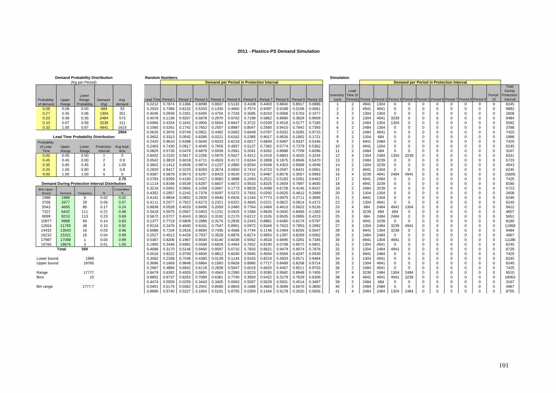
2011 - Plastics-PS Demand Simulation

Random Numbers Simulation

Lead Time Period 1 Period 2 Period 3 Period 4 Period 5 Period 6 Period 7 Period 8 Period 9 Period 10Inventory

cycle

Lead Time (# Periods) Period 1 Period 2 Period 3 Period 4 Period 5 Period 6 Period 7 Period 8 Period 9

Period 10

Total During

Protection Interval

0.0212 0.7874 0.1366 0.8098 0.8007 0.5132 0.4108 0.4403 0.8840 0.8917 0.0886 1 2 4941 1304 0 0 0 0 0 0 0 0 62450.08 0.08 0.00 684 53 0.2933 0.7386 0.8132 0.5333 0.1430 0.4660 0.7574 0.9497 0.9188 0.0158 0.0661 2 2 4941 4941 0 0 0 0 0 0 0 0 98820.27 0.35 0.08 1304 351 0.4046 0.0939 0.2351 0.6495 0.4704 0.7243 0.3585 0.8243 0.0068 0.5763 0.1077 3 2 1304 1304 0 0 0 0 0 0 0 0 26080.23 0.58 0.35 2484 573 0.4578 0.1136 0.9257 0.5878 0.2970 0.9702 0.7198 0.5862 0.8690 0.3829 0.9009 4 3 1304 4941 3239 0 0 0 0 0 0 0 94840.10 0.67 0.58 3239 311 0.6966 0.4334 0.1641 0.0906 0.5564 0.6647 0.3722 0.0339 0.4518 0.0177 0.7185 5 3 2484 1304 1304 0 0 0 0 0 0 0 50920.33 1.00 0.67 4941 1615 0.1060 0.5261 0.1742 0.7652 0.2557 0.8987 0.8047 0.2560 0.9410 0.7642 0.7393 6 2 2484 1304 0 0 0 0 0 0 0 0 3788

2904 0.0635 0.3976 0.9749 0.0921 0.4482 0.0692 0.6649 0.0787 0.6332 0.0285 0.9715 7 2 2484 4941 0 0 0 0 0 0 0 0 74250.3652 0.3313 0.0542 0.8285 0.0221 0.6162 0.2385 0.9017 0.9526 0.1802 0.1721 8 2 1304 684 0 0 0 0 0 0 0 0 19880.2420 0.9610 0.5398 0.5640 0.5533 0.6219 0.0917 0.6849 0.9487 0.9337 0.5346 9 2 4941 2484 0 0 0 0 0 0 0 0 74250.2463 0.7430 0.0917 0.4040 0.7656 0.4837 0.5137 0.7365 0.5774 0.7379 0.5362 10 2 4941 1304 0 0 0 0 0 0 0 0 62450.0825 0.5726 0.0478 0.6879 0.5939 0.2561 0.2041 0.9262 0.8588 0.7709 0.6096 11 2 2484 684 0 0 0 0 0 0 0 0 3167

0.00 0.00 0.00 1 0 0.8452 0.2220 0.5617 0.2256 0.5976 0.5627 0.4312 0.2419 0.6803 0.4020 0.3244 12 4 1304 2484 1304 3239 0 0 0 0 0 0 83310.45 0.45 0.00 2 0.9 0.0542 0.3819 0.6018 0.4711 0.4503 0.4172 0.6244 0.1808 0.1875 0.6946 0.5470 13 2 2484 3239 0 0 0 0 0 0 0 0 57230.35 0.80 0.45 3 1.05 0.3602 0.1412 0.6506 0.9974 0.1237 0.2880 0.9294 0.5048 0.4303 0.9069 0.4049 14 2 1304 3239 0 0 0 0 0 0 0 0 45430.20 1.00 0.80 4 0.8 0.2820 0.9417 0.3225 0.8283 0.3574 0.0650 0.7410 0.4723 0.2597 0.8431 0.0061 15 2 4941 1304 0 0 0 0 0 0 0 0 62450.00 1.00 1.00 5 0 0.9387 0.5876 0.9573 0.5297 0.8423 0.9520 0.5731 0.9487 0.8579 0.3057 0.9993 16 4 3239 4941 2484 4941 0 0 0 0 0 0 15605

2.75 0.0783 0.9359 0.4190 0.0427 0.9083 0.3888 0.2493 0.2522 0.5183 0.0281 0.6463 17 2 4941 2484 0 0 0 0 0 0 0 0 74250.1114 0.8166 0.6539 0.6287 0.6607 0.6672 0.9533 0.8325 0.2659 0.7697 0.4935 18 2 4941 3239 0 0 0 0 0 0 0 0 81800.3216 0.5092 0.5855 0.1058 0.0067 0.1773 0.8829 0.4098 0.6728 0.4145 0.9422 19 2 2484 3239 0 0 0 0 0 0 0 0 57230.4352 0.2557 0.2242 0.7378 0.9297 0.5372 0.7915 0.0292 0.0025 0.4612 0.2689 20 2 1304 1304 0 0 0 0 0 0 0 0 2608

1988 1988 8 0.02 0.02 0.4141 0.9834 0.0852 0.2835 0.9540 0.6926 0.1244 0.7773 0.5975 0.2711 0.3695 21 2 4941 1304 0 0 0 0 0 0 0 0 62453766 2877 28 0.06 0.07 0.4111 0.2077 0.7922 0.6273 0.2321 0.6322 0.4845 0.0221 0.0622 0.0814 0.4372 22 2 1304 4941 0 0 0 0 0 0 0 0 62455543 4655 85 0.17 0.24 0.8838 0.0528 0.4033 0.8496 0.2059 0.2480 0.7764 0.3469 0.4613 0.5622 0.9126 23 4 684 2484 4941 1304 0 0 0 0 0 0 94127321 6432 111 0.22 0.46 0.5418 0.5975 0.0567 0.0453 0.1231 0.0915 0.1584 0.9639 0.0400 0.8490 0.1383 24 3 3239 684 684 0 0 0 0 0 0 0 46079099 8210 113 0.23 0.69 0.5672 0.0727 0.4043 0.3653 0.3192 0.2170 0.6212 0.1535 0.9535 0.0995 0.4223 25 3 684 2484 2484 0 0 0 0 0 0 0 565110877 9988 69 0.14 0.83 0.1377 0.7719 0.5809 0.2886 0.3174 0.2835 0.2343 0.8881 0.6480 0.6174 0.5797 26 2 4941 3239 0 0 0 0 0 0 0 0 818012654 11765 48 0.10 0.92 0.9124 0.2476 0.4940 0.6341 0.7547 0.8901 0.0972 0.8349 0.7622 0.7853 0.2992 27 4 1304 2484 3239 4941 0 0 0 0 0 0 1196814432 13543 16 0.03 0.96 0.6986 0.7104 0.2616 0.6694 0.7435 0.4566 0.7744 0.1146 0.2464 0.8255 0.5547 28 3 4941 1304 3239 0 0 0 0 0 0 0 948416210 15321 18 0.04 0.99 0.2527 0.4012 0.4428 0.7937 0.3528 0.8876 0.8274 0.9953 0.1397 0.8269 0.0062 29 2 2484 2484 0 0 0 0 0 0 0 0 496717987 17098 1 0.00 0.99 0.5367 0.8206 0.1967 0.9030 0.6140 0.6038 0.5552 0.4533 0.8495 0.3291 0.7345 30 3 4941 1304 4941 0 0 0 0 0 0 0 1118619765 18876 3 0.01 1.00 0.1900 0.3446 0.6991 0.5568 0.6828 0.4464 0.7652 0.8190 0.0708 0.8072 0.5601 31 2 1304 4941 0 0 0 0 0 0 0 0 6245

Total 500 0.4686 0.3170 0.5146 0.9460 0.9597 0.0715 0.7833 0.8621 0.9479 0.9074 0.7876 32 3 1304 2484 4941 0 0 0 0 0 0 0 87290.0016 0.8222 0.3700 0.6830 0.9812 0.8240 0.5945 0.4004 0.5569 0.4247 0.5539 33 2 4941 2484 0 0 0 0 0 0 0 0 7425

Lower bound 1988 0.3562 0.2338 0.7048 0.4360 0.0139 0.1144 0.9163 0.8219 0.4933 0.0571 0.9484 34 2 1304 4941 0 0 0 0 0 0 0 0 6245Upper bound 19765 0.3696 0.1669 0.9848 0.6864 0.1583 0.6626 0.8980 0.7717 0.8489 0.8258 0.5714 35 2 1304 4941 0 0 0 0 0 0 0 0 6245

0.2967 0.4884 0.6942 0.6118 0.2838 0.5847 0.6018 0.6620 0.4467 0.9511 0.9703 36 2 2484 4941 0 0 0 0 0 0 0 0 7425Range 17777 0.8479 0.6392 0.4003 0.0891 0.4563 0.2390 0.9223 0.9280 0.9582 0.8948 0.7405 37 4 3239 2484 1304 2484 0 0 0 0 0 0 9510Bins 10 0.8852 0.9737 0.8253 0.7089 0.6361 0.7740 0.3593 0.5422 0.3179 0.7629 0.6309 38 4 4941 4941 4941 3239 0 0 0 0 0 0 18063

0.4474 0.5559 0.0259 0.3443 0.3405 0.0063 0.5587 0.5029 0.5931 0.4514 0.3497 39 2 2484 684 0 0 0 0 0 0 0 0 3167Bin range 1777.7 0.0401 0.5179 0.5562 0.2041 0.8590 0.8843 0.1686 0.4663 0.3699 0.6570 0.3800 40 2 2484 2484 0 0 0 0 0 0 0 0 4967

0.8886 0.5740 0.5227 0.1954 0.5191 0.8755 0.0359 0.1344 0.9178 0.3020 0.5656 41 4 2484 2484 1304 2484 0 0 0 0 0 0 8755

Demand per Period in Protection IntervalDemand Probability Distribution

(Kg per Period)

Lead Time Probability Distribution

Probability of demand

Demand During Protection Interval Distribution

Demand (Kg)

Avg demand

Bins Upper Bound Demand Frequency %

Cumulative %

Demand per Period in Protection Interval

Upper Range

Lower Range

Probability

Avg lead-time

Probability of Lead

TimeUpper Range

Lower Range

Protection Interval

101

2012 - Plastics-PS Demand Simulation

Random Numbers Simulation

Lead Time Period 1 Period 2 Period 3 Period 4 Period 5 Period 6 Period 7 Period 8 Period 9 Period 10Inventory

cycle

Lead Time (# Periods) Period 1 Period 2 Period 3 Period 4 Period 5 Period 6 Period 7 Period 8 Period 9

Period 10

Total During

Protection Interval

0.5902 0.5109 0.6921 0.4085 0.5521 0.2082 0.5342 0.6616 0.3096 0.5017 0.4807 1 3 3453 5856 2408 0 0 0 0 0 0 0 117160.08 0.08 0.00 810 62 0.3293 0.4095 0.1236 0.8381 0.5421 0.9739 0.3825 0.7835 0.5422 0.7836 0.6762 2 2 2408 1545 0 0 0 0 0 0 0 0 39530.27 0.35 0.08 1545 416 0.1925 0.1229 0.2448 0.2061 0.0233 0.8132 0.4254 0.6584 0.8154 0.7291 0.0633 3 2 1545 1545 0 0 0 0 0 0 0 0 30910.08 0.42 0.35 2408 185 0.1580 0.6418 0.7768 0.4237 0.4907 0.6148 0.3054 0.0414 0.0001 0.3800 0.5719 4 2 3453 5856 0 0 0 0 0 0 0 0 93090.25 0.67 0.42 3453 863 0.2968 0.6470 0.3470 0.4511 0.3439 0.4600 0.0025 0.8375 0.4384 0.4427 0.8782 5 2 3453 2408 0 0 0 0 0 0 0 0 58600.33 1.00 0.67 5856 1914 0.6727 0.3208 0.7052 0.8815 0.8443 0.3750 0.2078 0.5576 0.7913 0.2276 0.9644 6 3 1545 5856 5856 0 0 0 0 0 0 0 13258

3441 0.9523 0.1202 0.4656 0.0714 0.1947 0.3419 0.0198 0.1408 0.3182 0.4134 0.9673 7 4 1545 3453 810 1545 0 0 0 0 0 0 73540.2951 0.0770 0.9063 0.3440 0.0985 0.3839 0.7013 0.1165 0.7416 0.6526 0.0960 8 2 1545 5856 0 0 0 0 0 0 0 0 74020.3563 0.6584 0.4916 0.2491 0.0006 0.1915 0.5459 0.2304 0.4989 0.8854 0.4683 9 2 3453 3453 0 0 0 0 0 0 0 0 69060.8122 0.8816 0.9245 0.2625 0.2717 0.6579 0.5180 0.6465 0.4628 0.3876 0.2449 10 4 5856 5856 1545 1545 0 0 0 0 0 0 148030.9389 0.9443 0.6920 0.3076 0.2359 0.7170 0.2171 0.1160 0.7970 0.2664 0.5362 11 4 5856 5856 1545 1545 0 0 0 0 0 0 14803

0.00 0.00 0.00 1 0 0.3599 0.2260 0.4134 0.1691 0.1164 0.2343 0.7124 0.9203 0.3101 0.4623 0.8829 12 2 1545 2408 0 0 0 0 0 0 0 0 39530.45 0.45 0.00 2 0.9 0.2536 0.5657 0.3221 0.4864 0.2719 0.5406 0.2371 0.2175 0.9018 0.9366 0.7465 13 2 3453 1545 0 0 0 0 0 0 0 0 49980.35 0.80 0.45 3 1.05 0.1052 0.6020 0.3099 0.3429 0.4439 0.4409 0.2983 0.0608 0.7513 0.4012 0.0254 14 2 3453 1545 0 0 0 0 0 0 0 0 49980.20 1.00 0.80 4 0.8 0.6328 0.8275 0.2302 0.6685 0.4063 0.0123 0.8816 0.4515 0.5304 0.4838 0.6646 15 3 5856 1545 3453 0 0 0 0 0 0 0 108540.00 1.00 1.00 5 0 0.7103 0.3771 0.4715 0.3781 0.6076 0.0923 0.8871 0.2949 0.9517 0.3123 0.5842 16 3 2408 3453 2408 0 0 0 0 0 0 0 8268

2.75 0.8465 0.2052 0.2282 0.6889 0.3923 0.6101 0.2501 0.5074 0.4899 0.0687 0.4607 17 4 1545 1545 5856 2408 0 0 0 0 0 0 113550.3691 0.1877 0.6873 0.3220 0.4620 0.3858 0.8115 0.6694 0.5663 0.3622 0.7121 18 2 1545 5856 0 0 0 0 0 0 0 0 74020.5484 0.9770 0.6034 0.2065 0.9989 0.3611 0.2615 0.4912 0.6297 0.5807 0.5323 19 3 5856 3453 1545 0 0 0 0 0 0 0 108540.1843 0.3821 0.4772 0.3010 0.0595 0.1071 0.3445 0.1207 0.2567 0.7672 0.2776 20 2 2408 3453 0 0 0 0 0 0 0 0 5860

1621 1621 1 0.00 0.00 0.9494 0.9700 0.2731 0.4657 0.3363 0.4679 0.8502 0.6718 0.8834 0.1409 0.0358 21 4 5856 1545 3453 1545 0 0 0 0 0 0 124003801 2711 28 0.06 0.06 0.0645 0.4311 0.9131 0.9997 0.2744 0.6141 0.8443 0.9246 0.2786 0.1068 0.3823 22 2 3453 5856 0 0 0 0 0 0 0 0 93095982 4891 75 0.15 0.21 0.8281 0.9681 0.7363 0.6205 0.8236 0.3125 0.5961 0.0060 0.0462 0.2551 0.1821 23 4 5856 5856 3453 5856 0 0 0 0 0 0 210218162 7072 89 0.18 0.39 0.4672 0.1600 0.7218 0.6416 0.8256 0.6614 0.4264 0.7259 0.1784 0.9415 0.4632 24 3 1545 5856 3453 0 0 0 0 0 0 0 1085410342 9252 105 0.21 0.60 0.0797 0.7948 0.8304 0.7301 0.4935 0.9271 0.4176 0.5747 0.5578 0.1714 0.0384 25 2 5856 5856 0 0 0 0 0 0 0 0 1171212523 11432 80 0.16 0.76 0.7827 0.6668 0.6110 0.1958 0.6662 0.6205 0.0994 0.5669 0.4815 0.7404 0.0906 26 3 3453 3453 1545 0 0 0 0 0 0 0 845114703 13613 47 0.09 0.85 0.2108 0.1123 0.1667 0.9010 0.7720 0.9102 0.0860 0.2027 0.5469 0.9662 0.3979 27 2 1545 1545 0 0 0 0 0 0 0 0 309116883 15793 46 0.09 0.94 0.5519 0.7156 0.6759 0.1168 0.6466 0.9817 0.7652 0.1034 0.8693 0.0595 0.3749 28 3 5856 5856 1545 0 0 0 0 0 0 0 1325819063 17973 10 0.02 0.96 0.6270 0.5112 0.4312 0.3426 0.3963 0.7269 0.8056 0.2382 0.2806 0.9718 0.8763 29 3 3453 3453 1545 0 0 0 0 0 0 0 845121244 20154 16 0.03 0.99 0.3894 0.9603 0.7769 0.6384 0.1482 0.7965 0.6073 0.6547 0.8953 0.9343 0.7761 30 2 5856 5856 0 0 0 0 0 0 0 0 1171223424 22334 3 0.01 1.00 0.1326 0.4846 0.6498 0.7515 0.0090 0.6586 0.3688 0.0818 0.5412 0.6336 0.1458 31 2 3453 3453 0 0 0 0 0 0 0 0 6906

Total 500 0.1176 0.1766 0.8554 0.0205 0.7118 0.5285 0.8804 0.2214 0.7975 0.0499 0.1936 32 2 1545 5856 0 0 0 0 0 0 0 0 74020.2787 0.2745 0.7201 0.3158 0.6795 0.5654 0.5155 0.9651 0.2125 0.4614 0.8875 33 2 1545 5856 0 0 0 0 0 0 0 0 7402

Lower bound 1621 0.3591 0.8096 0.5780 0.2813 0.4311 0.2806 0.6825 0.6062 0.9149 0.0652 0.7860 34 2 5856 3453 0 0 0 0 0 0 0 0 9309Upper bound 23424 0.2441 0.5667 0.5727 0.2127 0.1720 0.0219 0.4007 0.5989 0.3710 0.2188 0.7084 35 2 3453 3453 0 0 0 0 0 0 0 0 6906

0.6822 0.9928 0.6916 0.2055 0.0080 0.4203 0.4680 0.0810 0.2793 0.6371 0.9197 36 3 5856 5856 1545 0 0 0 0 0 0 0 13258Range 21803 0.5948 0.8915 0.4353 0.6020 0.8502 0.5004 0.8595 0.4772 0.1103 0.7463 0.4822 37 3 5856 3453 3453 0 0 0 0 0 0 0 12762Bins 10 0.1573 0.9402 0.2686 0.5179 0.3639 0.9362 0.3393 0.1662 0.0835 0.6275 0.2466 38 2 5856 1545 0 0 0 0 0 0 0 0 7402

0.1528 0.7552 0.0790 0.9527 0.3127 0.4773 0.3469 0.4504 0.3661 0.0632 0.9104 39 2 5856 1545 0 0 0 0 0 0 0 0 7402Bin range 2180.3 0.8066 0.7264 0.9714 0.9587 0.1750 0.7324 0.2500 0.5080 0.7921 0.5744 0.1874 40 4 5856 5856 5856 1545 0 0 0 0 0 0 19114

0.4326 0.9364 0.9182 0.4582 0.0461 0.7775 0.8788 0.1446 0.8916 0.3585 0.6630 41 2 5856 5856 0 0 0 0 0 0 0 0 11712

Demand per Period in Protection IntervalDemand Probability Distribution

(Kg per Period)

Lead Time Probability Distribution

Probability of demand

Demand During Protection Interval Distribution

Demand (Kg)

Avg demand

Bins Upper Bound Demand Frequency %

Cumulative %

yof Lead

TimeLower Range

Protection Interval

Upper Range

Avg lead-time

Demand per Period in Protection Interval

Upper Range

Lower Range

Probability

102

Appendix II-B:

Plastic Sheets Demand Simulations

103

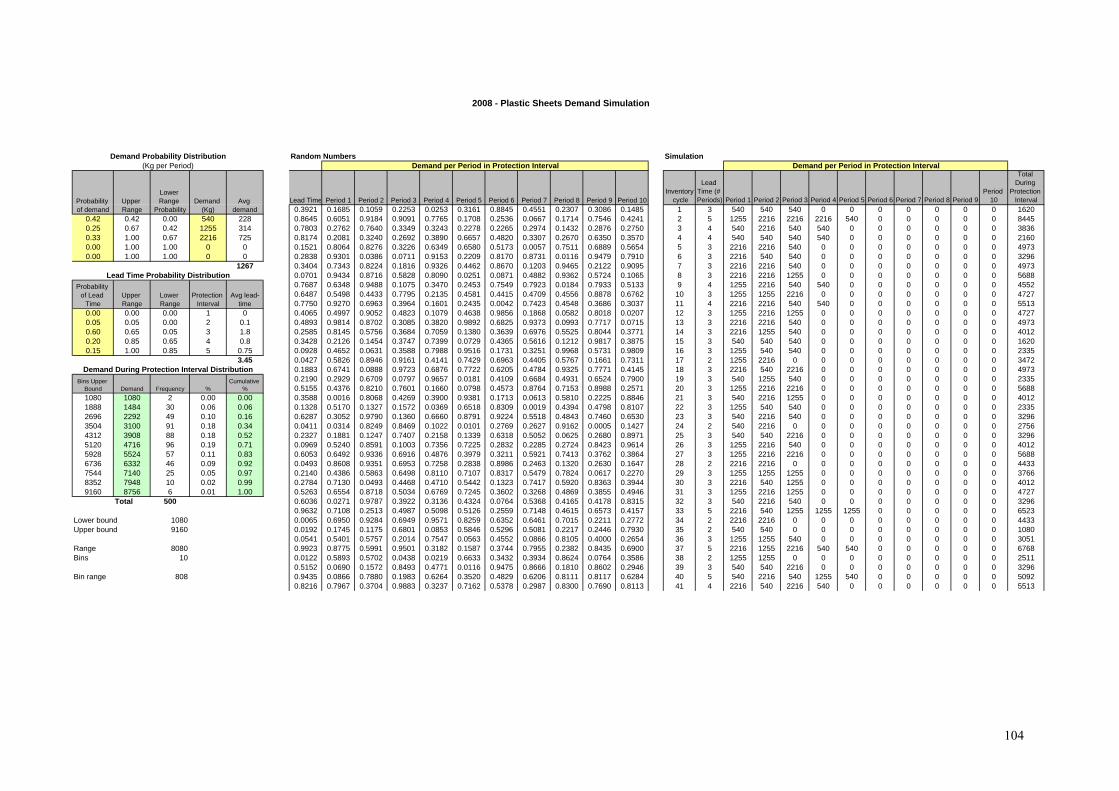
2008 - Plastic Sheets Demand Simulation

Random Numbers Simulation

Lead Time Period 1 Period 2 Period 3 Period 4 Period 5 Period 6 Period 7 Period 8 Period 9 Period 10Inventory

cycle

Lead Time (# Periods) Period 1 Period 2 Period 3 Period 4 Period 5 Period 6 Period 7 Period 8 Period 9

Period 10

Total During

Protection Interval

0.3921 0.1685 0.1059 0.2253 0.0253 0.3161 0.8845 0.4551 0.2307 0.3086 0.1485 1 3 540 540 540 0 0 0 0 0 0 0 16200.42 0.42 0.00 540 228 0.8645 0.6051 0.9184 0.9091 0.7765 0.1708 0.2536 0.0667 0.1714 0.7546 0.4241 2 5 1255 2216 2216 2216 540 0 0 0 0 0 84450.25 0.67 0.42 1255 314 0.7803 0.2762 0.7640 0.3349 0.3243 0.2278 0.2265 0.2974 0.1432 0.2876 0.2750 3 4 540 2216 540 540 0 0 0 0 0 0 38360.33 1.00 0.67 2216 725 0.8174 0.2081 0.3240 0.2692 0.3890 0.6657 0.4820 0.3307 0.2670 0.6350 0.3570 4 4 540 540 540 540 0 0 0 0 0 0 21600.00 1.00 1.00 0 0 0.1521 0.8064 0.8276 0.3226 0.6349 0.6580 0.5173 0.0057 0.7511 0.6889 0.5654 5 3 2216 2216 540 0 0 0 0 0 0 0 49730.00 1.00 1.00 0 0 0.2838 0.9301 0.0386 0.0711 0.9153 0.2209 0.8170 0.8731 0.0116 0.9479 0.7910 6 3 2216 540 540 0 0 0 0 0 0 0 3296

1267 0.3404 0.7343 0.8224 0.1816 0.9326 0.4462 0.8670 0.1203 0.9465 0.2122 0.9095 7 3 2216 2216 540 0 0 0 0 0 0 0 49730.0701 0.9434 0.8716 0.5828 0.8090 0.0251 0.0871 0.4882 0.9362 0.5724 0.1065 8 3 2216 2216 1255 0 0 0 0 0 0 0 56880.7687 0.6348 0.9488 0.1075 0.3470 0.2453 0.7549 0.7923 0.0184 0.7933 0.5133 9 4 1255 2216 540 540 0 0 0 0 0 0 45520.6487 0.5498 0.4433 0.7795 0.2135 0.4581 0.4415 0.4709 0.4556 0.8878 0.6762 10 3 1255 1255 2216 0 0 0 0 0 0 0 47270.7750 0.9270 0.6963 0.3964 0.1601 0.2435 0.0042 0.7423 0.4548 0.3686 0.3037 11 4 2216 2216 540 540 0 0 0 0 0 0 5513

0.00 0.00 0.00 1 0 0.4065 0.4997 0.9052 0.4823 0.1079 0.4638 0.9856 0.1868 0.0582 0.8018 0.0207 12 3 1255 2216 1255 0 0 0 0 0 0 0 47270.05 0.05 0.00 2 0.1 0.4893 0.9814 0.8702 0.3085 0.3820 0.9892 0.6825 0.9373 0.0993 0.7717 0.0715 13 3 2216 2216 540 0 0 0 0 0 0 0 49730.60 0.65 0.05 3 1.8 0.2585 0.8145 0.5756 0.3684 0.7059 0.1380 0.3639 0.6976 0.5525 0.8044 0.3771 14 3 2216 1255 540 0 0 0 0 0 0 0 40120.20 0.85 0.65 4 0.8 0.3428 0.2126 0.1454 0.3747 0.7399 0.0729 0.4365 0.5616 0.1212 0.9817 0.3875 15 3 540 540 540 0 0 0 0 0 0 0 16200.15 1.00 0.85 5 0.75 0.0928 0.4652 0.0631 0.3588 0.7988 0.9516 0.1731 0.3251 0.9968 0.5731 0.9809 16 3 1255 540 540 0 0 0 0 0 0 0 2335

3.45 0.0427 0.5826 0.8946 0.9161 0.4141 0.7429 0.6963 0.4405 0.5767 0.1661 0.7311 17 2 1255 2216 0 0 0 0 0 0 0 0 34720.1883 0.6741 0.0888 0.9723 0.6876 0.7722 0.6205 0.4784 0.9325 0.7771 0.4145 18 3 2216 540 2216 0 0 0 0 0 0 0 49730.2190 0.2929 0.6709 0.0797 0.9657 0.0181 0.4109 0.6684 0.4931 0.6524 0.7900 19 3 540 1255 540 0 0 0 0 0 0 0 23350.5155 0.4376 0.8210 0.7601 0.1660 0.0798 0.4573 0.8764 0.7153 0.8988 0.2571 20 3 1255 2216 2216 0 0 0 0 0 0 0 5688

1080 1080 2 0.00 0.00 0.3588 0.0016 0.8068 0.4269 0.3900 0.9381 0.1713 0.0613 0.5810 0.2225 0.8846 21 3 540 2216 1255 0 0 0 0 0 0 0 40121888 1484 30 0.06 0.06 0.1328 0.5170 0.1327 0.1572 0.0369 0.6518 0.8309 0.0019 0.4394 0.4798 0.8107 22 3 1255 540 540 0 0 0 0 0 0 0 23352696 2292 49 0.10 0.16 0.6287 0.3052 0.9790 0.1360 0.6660 0.8791 0.9224 0.5518 0.4843 0.7460 0.6530 23 3 540 2216 540 0 0 0 0 0 0 0 32963504 3100 91 0.18 0.34 0.0411 0.0314 0.8249 0.8469 0.1022 0.0101 0.2769 0.2627 0.9162 0.0005 0.1427 24 2 540 2216 0 0 0 0 0 0 0 0 27564312 3908 88 0.18 0.52 0.2327 0.1881 0.1247 0.7407 0.2158 0.1339 0.6318 0.5052 0.0625 0.2680 0.8971 25 3 540 540 2216 0 0 0 0 0 0 0 32965120 4716 96 0.19 0.71 0.0969 0.5240 0.8591 0.1003 0.7356 0.7225 0.2832 0.2285 0.2724 0.8423 0.9614 26 3 1255 2216 540 0 0 0 0 0 0 0 40125928 5524 57 0.11 0.83 0.6053 0.6492 0.9336 0.6916 0.4876 0.3979 0.3211 0.5921 0.7413 0.3762 0.3864 27 3 1255 2216 2216 0 0 0 0 0 0 0 56886736 6332 46 0.09 0.92 0.0493 0.8608 0.9351 0.6953 0.7258 0.2838 0.8986 0.2463 0.1320 0.2630 0.1647 28 2 2216 2216 0 0 0 0 0 0 0 0 44337544 7140 25 0.05 0.97 0.2140 0.4386 0.5863 0.6498 0.8110 0.7107 0.8317 0.5479 0.7824 0.0617 0.2270 29 3 1255 1255 1255 0 0 0 0 0 0 0 37668352 7948 10 0.02 0.99 0.2784 0.7130 0.0493 0.4468 0.4710 0.5442 0.1323 0.7417 0.5920 0.8363 0.3944 30 3 2216 540 1255 0 0 0 0 0 0 0 40129160 8756 6 0.01 1.00 0.5263 0.6554 0.8718 0.5034 0.6769 0.7245 0.3602 0.3268 0.4869 0.3855 0.4946 31 3 1255 2216 1255 0 0 0 0 0 0 0 4727

Total 500 0.6036 0.0271 0.9787 0.3922 0.3136 0.4324 0.0764 0.5368 0.4165 0.4178 0.8315 32 3 540 2216 540 0 0 0 0 0 0 0 32960.9632 0.7108 0.2513 0.4987 0.5098 0.5126 0.2559 0.7148 0.4615 0.6573 0.4157 33 5 2216 540 1255 1255 1255 0 0 0 0 0 6523

Lower bound 1080 0.0065 0.6950 0.9284 0.6949 0.9571 0.8259 0.6352 0.6461 0.7015 0.2211 0.2772 34 2 2216 2216 0 0 0 0 0 0 0 0 4433Upper bound 9160 0.0192 0.1745 0.1175 0.6801 0.0853 0.5846 0.5296 0.5081 0.2217 0.2446 0.7930 35 2 540 540 0 0 0 0 0 0 0 0 1080

0.0541 0.5401 0.5757 0.2014 0.7547 0.0563 0.4552 0.0866 0.8105 0.4000 0.2654 36 3 1255 1255 540 0 0 0 0 0 0 0 3051Range 8080 0.9923 0.8775 0.5991 0.9501 0.3182 0.1587 0.3744 0.7955 0.2382 0.8435 0.6900 37 5 2216 1255 2216 540 540 0 0 0 0 0 6768Bins 10 0.0122 0.5893 0.5702 0.0438 0.0219 0.6633 0.3432 0.3934 0.8624 0.0764 0.3586 38 2 1255 1255 0 0 0 0 0 0 0 0 2511

0.5152 0.0690 0.1572 0.8493 0.4771 0.0116 0.9475 0.8666 0.1810 0.8602 0.2946 39 3 540 540 2216 0 0 0 0 0 0 0 3296Bin range 808 0.9435 0.0866 0.7880 0.1983 0.6264 0.3520 0.4829 0.6206 0.8111 0.8117 0.6284 40 5 540 2216 540 1255 540 0 0 0 0 0 5092

0.8216 0.7967 0.3704 0.9883 0.3237 0.7162 0.5378 0.2987 0.8300 0.7690 0.8113 41 4 2216 540 2216 540 0 0 0 0 0 0 5513

Demand per Period in Protection IntervalDemand Probability Distribution

(Kg per Period)

Lead Time Probability Distribution

Probability of demand

Demand During Protection Interval Distribution

Demand (Kg)

Avg demand

Bins Upper Bound Demand Frequency %

Cumulative %

Demand per Period in Protection Interval

Upper Range

Lower Range

Probability

Avg lead-time

Probability of Lead

TimeUpper Range

Lower Range

Protection Interval

104

2009 - Plastic Sheets Demand Simulation

Random Numbers Simulation

Lead Time Period 1 Period 2 Period 3 Period 4 Period 5 Period 6 Period 7 Period 8 Period 9 Period 10Inventory

cycle

Lead Time (# Periods) Period 1 Period 2 Period 3 Period 4 Period 5 Period 6 Period 7 Period 8 Period 9

Period 10

Total During

Protection Interval

0.5005 0.9666 0.6244 0.8761 0.1215 0.4359 0.5547 0.2464 0.5680 0.5069 0.1174 1 3 3262 1619 3262 0 0 0 0 0 0 0 81430.35 0.35 0.00 502 174 0.2188 0.9338 0.9269 0.2800 0.1395 0.2917 0.8636 0.8547 0.3839 0.7784 0.8944 2 3 3262 3262 502 0 0 0 0 0 0 0 70270.33 0.67 0.35 1619 529 0.9368 0.6227 0.1462 0.0882 0.4042 0.8382 0.1818 0.4476 0.7440 0.7648 0.9144 3 5 1619 502 502 1619 2683 0 0 0 0 0 69250.17 0.85 0.67 2683 464 0.9435 0.2251 0.4894 0.7681 0.9427 0.3571 0.8832 0.0981 0.5224 0.4812 0.8055 4 5 502 1619 2683 3262 1619 0 0 0 0 0 96850.15 1.00 0.85 3262 502 0.7400 0.9106 0.8145 0.4804 0.3396 0.9252 0.9081 0.1944 0.6879 0.6121 0.1540 5 4 3262 2683 1619 502 0 0 0 0 0 0 80660.00 1.00 1.00 0 0 0.6078 0.7611 0.0573 0.9732 0.7596 0.4627 0.5174 0.7262 0.3182 0.5228 0.6877 6 3 2683 502 3262 0 0 0 0 0 0 0 6448

1669 0.7182 0.6646 0.5813 0.0729 0.3105 0.5316 0.4299 0.2311 0.0052 0.4534 0.5321 7 4 1619 1619 502 502 0 0 0 0 0 0 42420.8317 0.8673 0.2413 0.7945 0.7955 0.4602 0.7219 0.5004 0.6213 0.7909 0.3177 8 4 3262 502 2683 2683 0 0 0 0 0 0 91310.7897 0.2748 0.8934 0.4411 0.6594 0.9135 0.9702 0.8782 0.0877 0.5761 0.3477 9 4 502 3262 1619 1619 0 0 0 0 0 0 70020.2284 0.9825 0.0995 0.4866 0.0974 0.4211 0.2649 0.0987 0.0472 0.8658 0.7943 10 3 3262 502 1619 0 0 0 0 0 0 0 53830.6101 0.1783 0.7571 0.3852 0.0283 0.2261 0.6304 0.0755 0.6449 0.8447 0.0717 11 3 502 2683 1619 0 0 0 0 0 0 0 4804

0.00 0.00 0.00 1 0 0.2262 0.0389 0.5942 0.0168 0.1944 0.5437 0.5753 0.2677 0.6191 0.8509 0.6145 12 3 502 1619 502 0 0 0 0 0 0 0 26230.05 0.05 0.00 2 0.1 0.0619 0.8377 0.2457 0.7465 0.5949 0.7899 0.3626 0.7608 0.9913 0.8969 0.0751 13 3 2683 502 2683 0 0 0 0 0 0 0 58690.60 0.65 0.05 3 1.8 0.9903 0.0704 0.3528 0.3858 0.0172 0.7386 0.3211 0.9694 0.3144 0.3576 0.4117 14 5 502 1619 1619 502 2683 0 0 0 0 0 69250.20 0.85 0.65 4 0.8 0.7683 0.0047 0.0773 0.0998 0.3381 0.3200 0.3064 0.6047 0.4027 0.4688 0.3788 15 4 502 502 502 502 0 0 0 0 0 0 20090.15 1.00 0.85 5 0.75 0.5166 0.2587 0.7073 0.7851 0.2098 0.5948 0.6845 0.7446 0.6952 0.8252 0.4038 16 3 502 2683 2683 0 0 0 0 0 0 0 5869

3.45 0.5088 0.9540 0.1645 0.4243 0.7789 0.8520 0.4028 0.6393 0.8639 0.8058 0.3402 17 3 3262 502 1619 0 0 0 0 0 0 0 53830.7784 0.9614 0.2077 0.9069 0.5367 0.7683 0.8477 0.1824 0.5881 0.4568 0.6353 18 4 3262 502 3262 1619 0 0 0 0 0 0 86450.2903 0.6186 0.7540 0.5149 0.8282 0.6078 0.8502 0.4970 0.2919 0.2144 0.8084 19 3 1619 2683 1619 0 0 0 0 0 0 0 59200.5940 0.1637 0.2759 0.3916 0.8501 0.5821 0.6512 0.7677 0.3572 0.5241 0.3423 20 3 502 502 1619 0 0 0 0 0 0 0 2623

1004 1004 0 0.00 0.00 0.1013 0.0451 0.0760 0.4263 0.7548 0.3512 0.5935 0.8480 0.6678 0.1315 0.9865 21 3 502 502 1619 0 0 0 0 0 0 0 26232151 1577 23 0.05 0.05 0.4992 0.6535 0.6422 0.0045 0.0377 0.4394 0.1152 0.9166 0.7395 0.4666 0.9336 22 3 1619 1619 502 0 0 0 0 0 0 0 37393297 2724 45 0.09 0.14 0.3281 0.8983 0.7975 0.9445 0.1283 0.3489 0.0568 0.8857 0.7446 0.3109 0.8744 23 3 3262 2683 3262 0 0 0 0 0 0 0 92084444 3871 77 0.15 0.29 0.6607 0.7840 0.4580 0.3229 0.3631 0.0734 0.0997 0.8491 0.3454 0.4101 0.6832 24 4 2683 1619 502 1619 0 0 0 0 0 0 64235590 5017 100 0.20 0.49 0.3160 0.8676 0.0055 0.2187 0.2063 0.6333 0.6896 0.8735 0.5063 0.7929 0.3773 25 3 3262 502 502 0 0 0 0 0 0 0 42676737 6164 92 0.18 0.67 0.6163 0.6674 0.3787 0.9951 0.3956 0.7021 0.2156 0.4446 0.6337 0.9275 0.3898 26 3 1619 1619 3262 0 0 0 0 0 0 0 64997884 7310 57 0.11 0.79 0.9559 0.2601 0.9720 0.9547 0.0378 0.4996 0.0389 0.0164 0.6729 0.2844 0.1014 27 5 502 3262 3262 502 1619 0 0 0 0 0 91489030 8457 45 0.09 0.88 0.3090 0.3817 0.8706 0.2915 0.7464 0.6311 0.4437 0.2242 0.1614 0.7755 0.1824 28 3 1619 3262 502 0 0 0 0 0 0 0 5383

10177 9604 39 0.08 0.96 0.2312 0.3820 0.0453 0.1919 0.2320 0.2886 0.0930 0.5635 0.8954 0.1015 0.8067 29 3 1619 502 502 0 0 0 0 0 0 0 262311323 10750 12 0.02 0.98 0.0192 0.5754 0.6560 0.2944 0.4219 0.4882 0.9255 0.1614 0.2050 0.8012 0.7181 30 2 1619 1619 0 0 0 0 0 0 0 0 323712470 11897 10 0.02 1.00 0.1932 0.4770 0.2914 0.1177 0.6754 0.5930 0.8347 0.8304 0.7218 0.2678 0.1482 31 3 1619 502 502 0 0 0 0 0 0 0 2623

Total 500 0.4959 0.8510 0.7973 0.7941 0.4826 0.6658 0.3630 0.5406 0.5822 0.0393 0.0148 32 3 3262 2683 2683 0 0 0 0 0 0 0 86290.1156 0.6865 0.0764 0.4986 0.8007 0.4998 0.7913 0.1465 0.6098 0.9304 0.8202 33 3 2683 502 1619 0 0 0 0 0 0 0 4804

Lower bound 1004 0.4172 0.0913 0.1226 0.2353 0.4385 0.5317 0.5465 0.0161 0.6783 0.7146 0.6617 34 3 502 502 502 0 0 0 0 0 0 0 1507Upper bound 12470 0.8097 0.5759 0.0932 0.7607 0.3419 0.3746 0.4702 0.2289 0.6631 0.3608 0.9023 35 4 1619 502 2683 502 0 0 0 0 0 0 5306

0.9469 0.7516 0.0052 0.2195 0.9712 0.9281 0.4141 0.1587 0.8384 0.2983 0.1485 36 5 2683 502 502 3262 3262 0 0 0 0 0 10212Range 11466 0.3618 0.7929 0.4321 0.3690 0.6945 0.9490 0.4445 0.5948 0.1314 0.4777 0.7254 37 3 2683 1619 1619 0 0 0 0 0 0 0 5920Bins 10 0.4612 0.9990 0.6782 0.7700 0.4956 0.4514 0.6486 0.4095 0.9317 0.5970 0.7218 38 3 3262 2683 2683 0 0 0 0 0 0 0 8629

0.5913 0.7100 0.2383 0.3095 0.3643 0.5188 0.9429 0.2082 0.6506 0.2989 0.8927 39 3 2683 502 502 0 0 0 0 0 0 0 3688Bin range 1146.6 0.7658 0.9312 0.1596 0.2184 0.9261 0.8826 0.0443 0.3492 0.5783 0.8798 0.5450 40 4 3262 502 502 3262 0 0 0 0 0 0 7529

0.3307 0.0634 0.2418 0.6329 0.1724 0.6588 0.4419 0.4055 0.2598 0.3847 0.2510 41 3 502 502 1619 0 0 0 0 0 0 0 2623

Demand per Period in Protection IntervalDemand Probability Distribution

(Kg per Period)

Lead Time Probability Distribution

Probability of demand

Demand During Protection Interval Distribution

Demand (Kg)

Avg demand

Bins Upper Bound Demand Frequency %

Cumulative %

Demand per Period in Protection Interval

Upper Range

Lower Range

Probability

Avg lead-time

Probability of Lead

TimeUpper Range

Lower Range

Protection Interval

105

2010 - Plastic Sheets Demand Simulation

Random Numbers Simulation

Lead Time Period 1 Period 2 Period 3 Period 4 Period 5 Period 6 Period 7 Period 8 Period 9 Period 10Inventory

cycle

Lead Time (# Periods) Period 1 Period 2 Period 3 Period 4 Period 5 Period 6 Period 7 Period 8 Period 9

Period 10

Total During

Protection Interval

0.2115 0.9577 0.6460 0.1732 0.6346 0.7948 0.2538 0.0652 0.6482 0.9450 0.0731 1 3 4222 2379 1422 0 0 0 0 0 0 0 80220.1730769 0.17 0.00 698 121 0.0797 0.6431 0.4840 0.3978 0.6246 0.3088 0.2251 0.9597 0.5090 0.6887 0.1050 2 3 2379 1422 1422 0 0 0 0 0 0 0 5222

0.33 0.50 0.17 1422 465 0.9299 0.0185 0.8490 0.4853 0.6437 0.0484 0.9456 0.1726 0.2628 0.2734 0.3645 3 5 698 4222 1422 2379 698 0 0 0 0 0 94170.17 0.67 0.50 2379 412 0.9878 0.9999 0.2640 0.6191 0.2141 0.2296 0.0902 0.3076 0.6930 0.4627 0.0260 4 5 4222 1422 2379 1422 1422 0 0 0 0 0 108650.17 0.85 0.67 3472 601 0.0628 0.2076 0.0760 0.6458 0.3421 0.2222 0.9934 0.6268 0.6941 0.7018 0.4309 5 3 1422 698 2379 0 0 0 0 0 0 0 44980.15 1.00 0.85 4222 649 0.5810 0.1170 0.5652 0.9349 0.8006 0.2483 0.1690 0.9028 0.5642 0.9743 0.9890 6 3 698 2379 4222 0 0 0 0 0 0 0 7298

2248 0.7206 0.9388 0.4636 0.5774 0.0176 0.3958 0.9610 0.8837 0.8318 0.1379 0.7680 7 4 4222 1422 2379 698 0 0 0 0 0 0 87200.9616 0.0010 0.7851 0.7563 0.9951 0.8771 0.8628 0.6104 0.8228 0.0983 0.1127 8 5 698 3472 3472 4222 4222 0 0 0 0 0 160850.1251 0.7215 0.1557 0.3910 0.1469 0.1046 0.2585 0.2902 0.0866 0.7499 0.9339 9 3 3472 698 1422 0 0 0 0 0 0 0 55910.7007 0.8374 0.3636 0.0781 0.1027 0.4971 0.5170 0.7055 0.2036 0.3790 0.4199 10 4 3472 1422 698 698 0 0 0 0 0 0 62890.5211 0.9326 0.4981 0.8940 0.1730 0.7397 0.5205 0.4333 0.7145 0.0812 0.8596 11 3 4222 1422 4222 0 0 0 0 0 0 0 9865

0.00 0.00 0.00 1 0 0.9457 0.3097 0.3484 0.4868 0.4263 0.2661 0.7262 0.8667 0.5857 0.3329 0.0255 12 5 1422 1422 1422 1422 1422 0 0 0 0 0 71080.05 0.05 0.00 2 0.1 0.6645 0.7864 0.9268 0.8894 0.5922 0.0751 0.1513 0.4773 0.4847 0.0723 0.0847 13 4 3472 4222 4222 2379 0 0 0 0 0 0 142950.60 0.65 0.05 3 1.8 0.9008 0.3154 0.2097 0.1230 0.3018 0.2782 0.6630 0.6451 0.4094 0.1993 0.9329 14 5 1422 1422 698 1422 1422 0 0 0 0 0 63840.20 0.85 0.65 4 0.8 0.8866 0.7726 0.6188 0.4692 0.5983 0.3611 0.2372 0.5251 0.9272 0.1196 0.6003 15 5 3472 2379 1422 2379 1422 0 0 0 0 0 110740.15 1.00 0.85 5 0.75 0.4243 0.8409 0.4711 0.8915 0.7490 0.4510 0.1495 0.1408 0.7686 0.9136 0.6346 16 3 3472 1422 4222 0 0 0 0 0 0 0 9115

3.45 0.8684 0.3261 0.0472 0.2836 0.8132 0.3535 0.0191 0.4687 0.3057 0.2392 0.3102 17 5 1422 698 1422 3472 1422 0 0 0 0 0 84340.3616 0.1819 0.5159 0.7064 0.0737 0.4479 0.5646 0.7744 0.9543 0.1071 0.6680 18 3 1422 2379 3472 0 0 0 0 0 0 0 72730.5454 0.4287 0.0994 0.3558 0.6246 0.2342 0.1340 0.3075 0.0611 0.0774 0.7468 19 3 1422 698 1422 0 0 0 0 0 0 0 35410.6048 0.9685 0.0696 0.8360 0.7712 0.4492 0.4555 0.9551 0.6140 0.3876 0.5132 20 3 4222 698 3472 0 0 0 0 0 0 0 8391

1395 1395 0 0.00 0.00 0.4429 0.3772 0.2550 0.0632 0.3124 0.0375 0.3588 0.6067 0.3250 0.1452 0.3275 21 3 1422 1422 698 0 0 0 0 0 0 0 35412923 2159 18 0.04 0.04 0.7400 0.8000 0.0622 0.1697 0.7689 0.5937 0.6135 0.5629 0.2076 0.0318 0.4646 22 4 3472 698 698 3472 0 0 0 0 0 0 83404451 3687 43 0.09 0.12 0.6666 0.3313 0.6751 0.2325 0.7737 0.2833 0.5319 0.2020 0.6957 0.3598 0.1896 23 4 1422 3472 1422 3472 0 0 0 0 0 0 97885979 5215 69 0.14 0.26 0.2236 0.7609 0.6588 0.9085 0.8436 0.3663 0.5635 0.1738 0.9360 0.4610 0.5149 24 3 3472 2379 4222 0 0 0 0 0 0 0 100737507 6743 113 0.23 0.49 0.2883 0.9369 0.7473 0.5980 0.8888 0.8764 0.0384 0.5953 0.5167 0.0754 0.2955 25 3 4222 3472 2379 0 0 0 0 0 0 0 100739035 8271 78 0.16 0.64 0.3379 0.3321 0.0981 0.7101 0.2051 0.9971 0.9625 0.5090 0.2453 0.1937 0.7813 26 3 1422 698 3472 0 0 0 0 0 0 0 5591

10562 9798 88 0.18 0.82 0.2967 0.1978 0.8126 0.9104 0.2054 0.8169 0.2500 0.7440 0.3699 0.8812 0.2499 27 3 1422 3472 4222 0 0 0 0 0 0 0 911512090 11326 41 0.08 0.90 0.3641 0.5068 0.1216 0.8446 0.9956 0.6216 0.0785 0.2347 0.0895 0.5885 0.3407 28 3 2379 698 3472 0 0 0 0 0 0 0 654913618 12854 26 0.05 0.95 0.9434 0.5660 0.2574 0.0493 0.6823 0.1389 0.8317 0.6883 0.5277 0.4620 0.5881 29 5 2379 1422 698 3472 698 0 0 0 0 0 866815146 14382 17 0.03 0.99 0.5692 0.7225 0.9269 0.0204 0.9402 0.7098 0.2143 0.7932 0.5599 0.4124 0.5945 30 3 3472 4222 698 0 0 0 0 0 0 0 839116674 15910 7 0.01 1.00 0.8817 0.8357 0.5742 0.1200 0.9460 0.0962 0.2165 0.8099 0.8034 0.1487 0.5101 31 5 3472 2379 698 4222 698 0 0 0 0 0 11468

Total 500 0.5106 0.4606 0.0370 0.8808 0.2587 0.8766 0.1898 0.3828 0.5425 0.8476 0.0616 32 3 1422 698 4222 0 0 0 0 0 0 0 63410.1123 0.5207 0.1579 0.8292 0.7723 0.2715 0.8619 0.2835 0.4347 0.5434 0.9579 33 3 2379 698 3472 0 0 0 0 0 0 0 6549

Lower bound 1395 0.2537 0.4280 0.7785 0.8175 0.1514 0.3235 0.9503 0.7694 0.1710 0.4901 0.2800 34 3 1422 3472 3472 0 0 0 0 0 0 0 8366Upper bound 16674 0.8259 0.3825 0.2187 0.4220 0.4200 0.1497 0.8622 0.7003 0.4884 0.9940 0.3996 35 4 1422 1422 1422 1422 0 0 0 0 0 0 5686

0.5660 0.4648 0.0541 0.7100 0.9750 0.3449 0.7010 0.6357 0.2939 0.1032 0.0071 36 3 1422 698 3472 0 0 0 0 0 0 0 5591Range 15279 0.1314 0.2207 0.3463 0.0805 0.3047 0.8915 0.1813 0.3015 0.6304 0.6825 0.1686 37 3 1422 1422 698 0 0 0 0 0 0 0 3541Bins 10 0.7099 0.0702 0.5452 0.9090 0.5272 0.8205 0.5972 0.5226 0.1541 0.0141 0.4873 38 4 698 2379 4222 2379 0 0 0 0 0 0 9678

0.6997 0.4968 0.2124 0.8988 0.3698 0.7855 0.8921 0.5811 0.1109 0.4921 0.5798 39 4 1422 1422 4222 1422 0 0 0 0 0 0 8486Bin range 1527.9 0.9070 0.7060 0.9598 0.5580 0.4351 0.6438 0.7009 0.9090 0.1025 0.2002 0.9087 40 5 3472 4222 2379 1422 2379 0 0 0 0 0 13874

0.4936 0.3051 0.6889 0.1080 0.7741 0.2644 0.5346 0.4565 0.5269 0.7189 0.3594 41 3 1422 3472 698 0 0 0 0 0 0 0 5591

Demand per Period in Protection IntervalDemand Probability Distribution

(Kg per Period)

Lead Time Probability Distribution

Probability of demand

Demand During Protection Interval Distribution

Demand (Kg)

Avg demand

Bins Upper Bound Demand Frequency %

Cumulative %

Demand per Period in Protection Interval

Upper Range

Lower Range

Probability

Avg lead-time

Probability of Lead

TimeUpper Range

Lower Range

Protection Interval

106

2011 - Plastic Sheets Demand Simulation

Random Numbers Simulation

Lead Time Period 1 Period 2 Period 3 Period 4 Period 5 Period 6 Period 7 Period 8 Period 9 Period 10Inventory

cycle

Lead Time (# Periods) Period 1 Period 2 Period 3 Period 4 Period 5 Period 6 Period 7 Period 8 Period 9

Period 10

Total During

Protection Interval

0.0212 0.7874 0.1366 0.8098 0.8007 0.5132 0.4108 0.4403 0.8840 0.8917 0.0886 1 2 4986 1392 0 0 0 0 0 0 0 0 63780.08 0.08 0.00 649 50 0.2933 0.7386 0.8132 0.5333 0.1430 0.4660 0.7574 0.9497 0.9188 0.0158 0.0661 2 3 3536 4986 2574 0 0 0 0 0 0 0 110960.35 0.42 0.08 1392 482 0.4046 0.0939 0.2351 0.6495 0.4704 0.7243 0.3585 0.8243 0.0068 0.5763 0.1077 3 3 1392 1392 3536 0 0 0 0 0 0 0 63200.15 0.58 0.42 2574 396 0.4578 0.1136 0.9257 0.5878 0.2970 0.9702 0.7198 0.5862 0.8690 0.3829 0.9009 4 3 1392 4986 3536 0 0 0 0 0 0 0 99140.19 0.77 0.58 3536 680 0.6966 0.4334 0.1641 0.0906 0.5564 0.6647 0.3722 0.0339 0.4518 0.0177 0.7185 5 4 2574 1392 1392 2574 0 0 0 0 0 0 79330.23 1.00 0.77 4986 1151 0.1060 0.5261 0.1742 0.7652 0.2557 0.8987 0.8047 0.2560 0.9410 0.7642 0.7393 6 3 2574 1392 3536 0 0 0 0 0 0 0 7502

2758 0.0635 0.3976 0.9749 0.0921 0.4482 0.0692 0.6649 0.0787 0.6332 0.0285 0.9715 7 3 1392 4986 1392 0 0 0 0 0 0 0 77710.3652 0.3313 0.0542 0.8285 0.0221 0.6162 0.2385 0.9017 0.9526 0.1802 0.1721 8 3 1392 649 4986 0 0 0 0 0 0 0 70280.2420 0.9610 0.5398 0.5640 0.5533 0.6219 0.0917 0.6849 0.9487 0.9337 0.5346 9 3 4986 2574 2574 0 0 0 0 0 0 0 101340.2463 0.7430 0.0917 0.4040 0.7656 0.4837 0.5137 0.7365 0.5774 0.7379 0.5362 10 3 3536 1392 1392 0 0 0 0 0 0 0 63200.0825 0.5726 0.0478 0.6879 0.5939 0.2561 0.2041 0.9262 0.8588 0.7709 0.6096 11 3 2574 649 3536 0 0 0 0 0 0 0 6759

0.00 0.00 0.00 1 0 0.8452 0.2220 0.5617 0.2256 0.5976 0.5627 0.4312 0.2419 0.6803 0.4020 0.3244 12 4 1392 2574 1392 3536 0 0 0 0 0 0 88950.05 0.05 0.00 2 0.1 0.0542 0.3819 0.6018 0.4711 0.4503 0.4172 0.6244 0.1808 0.1875 0.6946 0.5470 13 3 1392 3536 2574 0 0 0 0 0 0 0 75020.60 0.65 0.05 3 1.8 0.3602 0.1412 0.6506 0.9974 0.1237 0.2880 0.9294 0.5048 0.4303 0.9069 0.4049 14 3 1392 3536 4986 0 0 0 0 0 0 0 99140.20 0.85 0.65 4 0.8 0.2820 0.9417 0.3225 0.8283 0.3574 0.0650 0.7410 0.4723 0.2597 0.8431 0.0061 15 3 4986 1392 4986 0 0 0 0 0 0 0 113640.15 1.00 0.85 5 0.75 0.9387 0.5876 0.9573 0.5297 0.8423 0.9520 0.5731 0.9487 0.8579 0.3057 0.9993 16 5 3536 4986 2574 4986 4986 0 0 0 0 0 21067

3.45 0.0783 0.9359 0.4190 0.0427 0.9083 0.3888 0.2493 0.2522 0.5183 0.0281 0.6463 17 3 4986 1392 649 0 0 0 0 0 0 0 70280.1114 0.8166 0.6539 0.6287 0.6607 0.6672 0.9533 0.8325 0.2659 0.7697 0.4935 18 3 4986 3536 3536 0 0 0 0 0 0 0 120570.3216 0.5092 0.5855 0.1058 0.0067 0.1773 0.8829 0.4098 0.6728 0.4145 0.9422 19 3 2574 3536 1392 0 0 0 0 0 0 0 75020.4352 0.2557 0.2242 0.7378 0.9297 0.5372 0.7915 0.0292 0.0025 0.4612 0.2689 20 3 1392 1392 3536 0 0 0 0 0 0 0 6320

2785 2785 3 0.01 0.01 0.4141 0.9834 0.0852 0.2835 0.9540 0.6926 0.1244 0.7773 0.5975 0.2711 0.3695 21 3 4986 1392 1392 0 0 0 0 0 0 0 77714709 3747 29 0.06 0.06 0.4111 0.2077 0.7922 0.6273 0.2321 0.6322 0.4845 0.0221 0.0622 0.0814 0.4372 22 3 1392 4986 3536 0 0 0 0 0 0 0 99146634 5672 80 0.16 0.22 0.8838 0.0528 0.4033 0.8496 0.2059 0.2480 0.7764 0.3469 0.4613 0.5622 0.9126 23 5 649 1392 4986 1392 1392 0 0 0 0 0 98138558 7596 115 0.23 0.45 0.5418 0.5975 0.0567 0.0453 0.1231 0.0915 0.1584 0.9639 0.0400 0.8490 0.1383 24 3 3536 649 649 0 0 0 0 0 0 0 4835

10483 9520 114 0.23 0.68 0.5672 0.0727 0.4043 0.3653 0.3192 0.2170 0.6212 0.1535 0.9535 0.0995 0.4223 25 3 649 1392 1392 0 0 0 0 0 0 0 343412407 11445 75 0.15 0.83 0.1377 0.7719 0.5809 0.2886 0.3174 0.2835 0.2343 0.8881 0.6480 0.6174 0.5797 26 3 4986 3536 1392 0 0 0 0 0 0 0 991414331 13369 38 0.08 0.91 0.9124 0.2476 0.4940 0.6341 0.7547 0.8901 0.0972 0.8349 0.7622 0.7853 0.2992 27 5 1392 2574 3536 3536 4986 0 0 0 0 0 1602416256 15294 28 0.06 0.96 0.6986 0.7104 0.2616 0.6694 0.7435 0.4566 0.7744 0.1146 0.2464 0.8255 0.5547 28 4 3536 1392 3536 3536 0 0 0 0 0 0 1199918180 17218 8 0.02 0.98 0.2527 0.4012 0.4428 0.7937 0.3528 0.8876 0.8274 0.9953 0.1397 0.8269 0.0062 29 3 1392 2574 4986 0 0 0 0 0 0 0 895220105 19142 5 0.01 0.99 0.5367 0.8206 0.1967 0.9030 0.6140 0.6038 0.5552 0.4533 0.8495 0.3291 0.7345 30 3 4986 1392 4986 0 0 0 0 0 0 0 1136422029 21067 5 0.01 1.00 0.1900 0.3446 0.6991 0.5568 0.6828 0.4464 0.7652 0.8190 0.0708 0.8072 0.5601 31 3 1392 3536 2574 0 0 0 0 0 0 0 7502

Total 500 0.4686 0.3170 0.5146 0.9460 0.9597 0.0715 0.7833 0.8621 0.9479 0.9074 0.7876 32 3 1392 2574 4986 0 0 0 0 0 0 0 89520.0016 0.8222 0.3700 0.6830 0.9812 0.8240 0.5945 0.4004 0.5569 0.4247 0.5539 33 2 4986 1392 0 0 0 0 0 0 0 0 6378

Lower bound 2785 0.3562 0.2338 0.7048 0.4360 0.0139 0.1144 0.9163 0.8219 0.4933 0.0571 0.9484 34 3 1392 3536 2574 0 0 0 0 0 0 0 7502Upper bound 22029 0.3696 0.1669 0.9848 0.6864 0.1583 0.6626 0.8980 0.7717 0.8489 0.8258 0.5714 35 3 1392 4986 3536 0 0 0 0 0 0 0 9914

0.2967 0.4884 0.6942 0.6118 0.2838 0.5847 0.6018 0.6620 0.4467 0.9511 0.9703 36 3 2574 3536 3536 0 0 0 0 0 0 0 9645Range 19244 0.8479 0.6392 0.4003 0.0891 0.4563 0.2390 0.9223 0.9280 0.9582 0.8948 0.7405 37 4 3536 1392 1392 2574 0 0 0 0 0 0 8895Bins 10 0.8852 0.9737 0.8253 0.7089 0.6361 0.7740 0.3593 0.5422 0.3179 0.7629 0.6309 38 5 4986 4986 3536 3536 4986 0 0 0 0 0 22029

0.4474 0.5559 0.0259 0.3443 0.3405 0.0063 0.5587 0.5029 0.5931 0.4514 0.3497 39 3 2574 649 1392 0 0 0 0 0 0 0 4616Bin range 1924.4 0.0401 0.5179 0.5562 0.2041 0.8590 0.8843 0.1686 0.4663 0.3699 0.6570 0.3800 40 2 2574 2574 0 0 0 0 0 0 0 0 5148

0.8886 0.5740 0.5227 0.1954 0.5191 0.8755 0.0359 0.1344 0.9178 0.3020 0.5656 41 5 2574 2574 1392 2574 4986 0 0 0 0 0 14101

Avg lead-time

Demand During Protection Interval Distribution

Demand (Kg)

Avg demand

Bins Upper Bound Demand Frequency %

Cumulative %

Upper Range

Lower Range

Probability

Demand per Period in Protection IntervalDemand Probability Distribution

(Kg per Period)

Lead Time Probability Distribution

Probability of demand

Demand per Period in Protection Interval

Probability of Lead

TimeUpper Range

Lower Range

Protection Interval

107

2012 - Plastic Sheets Demand Simulation

Random Numbers Simulation

Lead Time Period 1 Period 2 Period 3 Period 4 Period 5 Period 6 Period 7 Period 8 Period 9 Period 10Inventory

cycle

Lead Time (# Periods) Period 1 Period 2 Period 3 Period 4 Period 5 Period 6 Period 7 Period 8 Period 9

Period 10

Total During

Protection Interval

0.5902 0.5109 0.6921 0.4085 0.5521 0.2082 0.5342 0.6616 0.3096 0.5017 0.4807 1 3 3460 5563 2581 0 0 0 0 0 0 0 116050.08 0.08 0.00 770 59 0.3293 0.4095 0.1236 0.8381 0.5421 0.9739 0.3825 0.7835 0.5422 0.7836 0.6762 2 3 2581 1468 5563 0 0 0 0 0 0 0 96120.27 0.35 0.08 1468 395 0.1925 0.1229 0.2448 0.2061 0.0233 0.8132 0.4254 0.6584 0.8154 0.7291 0.0633 3 3 1468 1468 1468 0 0 0 0 0 0 0 44050.15 0.50 0.35 2581 397 0.1580 0.6418 0.7768 0.4237 0.4907 0.6148 0.3054 0.0414 0.0001 0.3800 0.5719 4 3 3460 5563 2581 0 0 0 0 0 0 0 116050.17 0.67 0.50 3460 599 0.2968 0.6470 0.3470 0.4511 0.3439 0.4600 0.0025 0.8375 0.4384 0.4427 0.8782 5 3 3460 2581 2581 0 0 0 0 0 0 0 86220.33 1.00 0.67 5563 1819 0.6727 0.3208 0.7052 0.8815 0.8443 0.3750 0.2078 0.5576 0.7913 0.2276 0.9644 6 4 1468 5563 5563 5563 0 0 0 0 0 0 18158

3269 0.9523 0.1202 0.4656 0.0714 0.1947 0.3419 0.0198 0.1408 0.3182 0.4134 0.9673 7 5 1468 2581 770 1468 1468 0 0 0 0 0 77550.2951 0.0770 0.9063 0.3440 0.0985 0.3839 0.7013 0.1165 0.7416 0.6526 0.0960 8 3 1468 5563 1468 0 0 0 0 0 0 0 85000.3563 0.6584 0.4916 0.2491 0.0006 0.1915 0.5459 0.2304 0.4989 0.8854 0.4683 9 3 3460 2581 1468 0 0 0 0 0 0 0 75090.8122 0.8816 0.9245 0.2625 0.2717 0.6579 0.5180 0.6465 0.4628 0.3876 0.2449 10 4 5563 5563 1468 1468 0 0 0 0 0 0 140630.9389 0.9443 0.6920 0.3076 0.2359 0.7170 0.2171 0.1160 0.7970 0.2664 0.5362 11 5 5563 5563 1468 1468 5563 0 0 0 0 0 19626

0.00 0.00 0.00 1 0 0.3599 0.2260 0.4134 0.1691 0.1164 0.2343 0.7124 0.9203 0.3101 0.4623 0.8829 12 3 1468 2581 1468 0 0 0 0 0 0 0 55170.05 0.05 0.00 2 0.1 0.2536 0.5657 0.3221 0.4864 0.2719 0.5406 0.2371 0.2175 0.9018 0.9366 0.7465 13 3 3460 1468 2581 0 0 0 0 0 0 0 75090.60 0.65 0.05 3 1.8 0.1052 0.6020 0.3099 0.3429 0.4439 0.4409 0.2983 0.0608 0.7513 0.4012 0.0254 14 3 3460 1468 1468 0 0 0 0 0 0 0 63970.20 0.85 0.65 4 0.8 0.6328 0.8275 0.2302 0.6685 0.4063 0.0123 0.8816 0.4515 0.5304 0.4838 0.6646 15 3 5563 1468 3460 0 0 0 0 0 0 0 104920.15 1.00 0.85 5 0.75 0.7103 0.3771 0.4715 0.3781 0.6076 0.0923 0.8871 0.2949 0.9517 0.3123 0.5842 16 4 2581 2581 2581 3460 0 0 0 0 0 0 11203

3.45 0.8465 0.2052 0.2282 0.6889 0.3923 0.6101 0.2501 0.5074 0.4899 0.0687 0.4607 17 4 1468 1468 5563 2581 0 0 0 0 0 0 110800.3691 0.1877 0.6873 0.3220 0.4620 0.3858 0.8115 0.6694 0.5663 0.3622 0.7121 18 3 1468 5563 1468 0 0 0 0 0 0 0 85000.5484 0.9770 0.6034 0.2065 0.9989 0.3611 0.2615 0.4912 0.6297 0.5807 0.5323 19 3 5563 3460 1468 0 0 0 0 0 0 0 104920.1843 0.3821 0.4772 0.3010 0.0595 0.1071 0.3445 0.1207 0.2567 0.7672 0.2776 20 3 2581 2581 1468 0 0 0 0 0 0 0 6630

2936 2936 0 0.00 0.00 0.9494 0.9700 0.2731 0.4657 0.3363 0.4679 0.8502 0.6718 0.8834 0.1409 0.0358 21 5 5563 1468 2581 1468 2581 0 0 0 0 0 136615214 4075 22 0.04 0.04 0.0645 0.4311 0.9131 0.9997 0.2744 0.6141 0.8443 0.9246 0.2786 0.1068 0.3823 22 3 2581 5563 5563 0 0 0 0 0 0 0 137077491 6353 45 0.09 0.13 0.8281 0.9681 0.7363 0.6205 0.8236 0.3125 0.5961 0.0060 0.0462 0.2551 0.1821 23 4 5563 5563 3460 5563 0 0 0 0 0 0 201509769 8630 137 0.27 0.41 0.4672 0.1600 0.7218 0.6416 0.8256 0.6614 0.4264 0.7259 0.1784 0.9415 0.4632 24 3 1468 5563 3460 0 0 0 0 0 0 0 1049212047 10908 93 0.19 0.59 0.0797 0.7948 0.8304 0.7301 0.4935 0.9271 0.4176 0.5747 0.5578 0.1714 0.0384 25 3 5563 5563 5563 0 0 0 0 0 0 0 1669014325 13186 75 0.15 0.74 0.7827 0.6668 0.6110 0.1958 0.6662 0.6205 0.0994 0.5669 0.4815 0.7404 0.0906 26 4 3460 3460 1468 3460 0 0 0 0 0 0 1185016602 15463 57 0.11 0.86 0.2108 0.1123 0.1667 0.9010 0.7720 0.9102 0.0860 0.2027 0.5469 0.9662 0.3979 27 3 1468 1468 5563 0 0 0 0 0 0 0 850018880 17741 36 0.07 0.93 0.5519 0.7156 0.6759 0.1168 0.6466 0.9817 0.7652 0.1034 0.8693 0.0595 0.3749 28 3 5563 5563 1468 0 0 0 0 0 0 0 1259521158 20019 22 0.04 0.97 0.6270 0.5112 0.4312 0.3426 0.3963 0.7269 0.8056 0.2382 0.2806 0.9718 0.8763 29 3 3460 2581 1468 0 0 0 0 0 0 0 750923435 22296 6 0.01 0.99 0.3894 0.9603 0.7769 0.6384 0.1482 0.7965 0.6073 0.6547 0.8953 0.9343 0.7761 30 3 5563 5563 3460 0 0 0 0 0 0 0 1458725713 24574 7 0.01 1.00 0.1326 0.4846 0.6498 0.7515 0.0090 0.6586 0.3688 0.0818 0.5412 0.6336 0.1458 31 3 2581 3460 5563 0 0 0 0 0 0 0 11605

Total 500 0.1176 0.1766 0.8554 0.0205 0.7118 0.5285 0.8804 0.2214 0.7975 0.0499 0.1936 32 3 1468 5563 770 0 0 0 0 0 0 0 78010.2787 0.2745 0.7201 0.3158 0.6795 0.5654 0.5155 0.9651 0.2125 0.4614 0.8875 33 3 1468 5563 1468 0 0 0 0 0 0 0 8500

Lower bound 2936 0.3591 0.8096 0.5780 0.2813 0.4311 0.2806 0.6825 0.6062 0.9149 0.0652 0.7860 34 3 5563 3460 1468 0 0 0 0 0 0 0 10492Upper bound 25713 0.2441 0.5667 0.5727 0.2127 0.1720 0.0219 0.4007 0.5989 0.3710 0.2188 0.7084 35 3 3460 3460 1468 0 0 0 0 0 0 0 8389

0.6822 0.9928 0.6916 0.2055 0.0080 0.4203 0.4680 0.0810 0.2793 0.6371 0.9197 36 4 5563 5563 1468 770 0 0 0 0 0 0 13364Range 22777 0.5948 0.8915 0.4353 0.6020 0.8502 0.5004 0.8595 0.4772 0.1103 0.7463 0.4822 37 3 5563 2581 3460 0 0 0 0 0 0 0 11605Bins 10 0.1573 0.9402 0.2686 0.5179 0.3639 0.9362 0.3393 0.1662 0.0835 0.6275 0.2466 38 3 5563 1468 3460 0 0 0 0 0 0 0 10492

0.1528 0.7552 0.0790 0.9527 0.3127 0.4773 0.3469 0.4504 0.3661 0.0632 0.9104 39 3 5563 1468 5563 0 0 0 0 0 0 0 12595Bin range 2277.7 0.8066 0.7264 0.9714 0.9587 0.1750 0.7324 0.2500 0.5080 0.7921 0.5744 0.1874 40 4 5563 5563 5563 1468 0 0 0 0 0 0 18158

0.4326 0.9364 0.9182 0.4582 0.0461 0.7775 0.8788 0.1446 0.8916 0.3585 0.6630 41 3 5563 5563 2581 0 0 0 0 0 0 0 13707

Avg lead-time

Demand During Protection Interval Distribution

Demand (Kg)

Avg demand

Bins Upper Bound Demand Frequency %

Cumulative %

Upper Range

Lower Range

Probability

Demand per Period in Protection IntervalDemand Probability Distribution

(Kg per Period)

Lead Time Probability Distribution

Probability of demand

Demand per Period in Protection Interval

Probability of Lead

TimeUpper Range

Lower Range

Protection Interval

108

Appendix III:

Weekly Demand Distribution

109

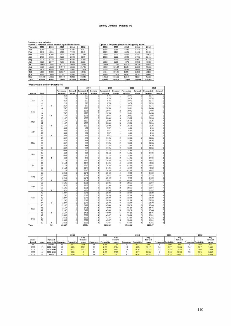
Weekly Demand - Plastics-PS

Inventory: raw materialsOption 1: Required plastic sheet in kg (half outsource) Option 2: Required plastic-PS in kg (fully made)Year/mth 2008 2009 2010 2011 2012 2008 2009 2010 2011 2012Jan 1040 3216 4161 5107 6052 1095 3385 4380 5376 6371Feb 2840 4861 6290 7720 9149 2989 5117 6621 8126 9630Mar 4360 6108 7905 9701 11497 4589 6430 8321 10212 12102Apr 1480 1636 2117 2598 3079 1558 1722 2228 2735 3241May 4000 4128 5342 6556 7769 4211 4345 5623 6901 8178Jun 2520 3577 4629 5681 6733 2653 3766 4873 5980 7088Jul 10040 12574 16272 19969 23667 10568 13236 17128 21020 24912Aug 9360 11575 14979 18383 21786 9853 12184 15767 19350 22933Sep 5800 6858 8875 10892 12909 6105 7219 9342 11465 13588Oct 6160 9688 12537 15386 18235 6484 10198 13197 16196 19195Nov 8160 13215 17101 20987 24874 8589 13911 18001 22092 26183Dec 10120 12883 16672 20460 24249 10653 13561 17549 21537 25525Total 65880 90320 116880 143440 170000 69347 95074 123032 150989 178947

Weekly Demand for Plastic-PS

Forecasted Demand

Demand Range

Forecasted Demand

Demand Range

Forecasted Demand

Demand Range

Forecasted Demand

Demand Range

Forecasted Demand

Demand Range

1 219 1 677 1 876 1 1075 2 1274 22 219 1 677 1 876 1 1075 2 1274 23 219 1 677 1 876 1 1075 2 1274 24 219 1 677 1 876 1 1075 2 1274 25 219 1 677 1 876 1 1075 2 1274 26 747 1 1279 2 1655 2 2031 3 2408 37 747 1 1279 2 1655 2 2031 3 2408 38 747 1 1279 2 1655 2 2031 3 2408 39 747 1 1279 2 1655 2 2031 3 2408 3

10 1147 2 1607 2 2080 3 2553 3 3026 411 1147 2 1607 2 2080 3 2553 3 3026 412 1147 2 1607 2 2080 3 2553 3 3026 413 1147 2 1607 2 2080 3 2553 3 3026 414 389 1 430 1 557 1 684 1 810 115 389 1 430 1 557 1 684 1 810 116 389 1 430 1 557 1 684 1 810 117 389 1 430 1 557 1 684 1 810 118 842 1 869 1 1125 2 1380 2 1636 219 842 1 869 1 1125 2 1380 2 1636 220 842 1 869 1 1125 2 1380 2 1636 221 842 1 869 1 1125 2 1380 2 1636 222 842 1 869 1 1125 2 1380 2 1636 223 663 1 941 1 1218 2 1495 2 1772 224 663 1 941 1 1218 2 1495 2 1772 225 663 1 941 1 1218 2 1495 2 1772 226 663 1 941 1 1218 2 1495 2 1772 227 2114 3 2647 3 3426 4 4204 5 4982 528 2114 3 2647 3 3426 4 4204 5 4982 529 2114 3 2647 3 3426 4 4204 5 4982 530 2114 3 2647 3 3426 4 4204 5 4982 531 2114 3 2647 3 3426 4 4204 5 4982 532 2463 3 3046 4 3942 4 4838 5 5733 533 2463 3 3046 4 3942 4 4838 5 5733 534 2463 3 3046 4 3942 4 4838 5 5733 535 2463 3 3046 4 3942 4 4838 5 5733 536 1526 2 1805 2 2336 3 2866 3 3397 437 1526 2 1805 2 2336 3 2866 3 3397 438 1526 2 1805 2 2336 3 2866 3 3397 439 1526 2 1805 2 2336 3 2866 3 3397 440 1297 2 2040 3 2639 3 3239 4 3839 441 1297 2 2040 3 2639 3 3239 4 3839 442 1297 2 2040 3 2639 3 3239 4 3839 443 1297 2 2040 3 2639 3 3239 4 3839 444 1297 2 2040 3 2639 3 3239 4 3839 445 2147 3 3478 4 4500 5 5523 5 6546 546 2147 3 3478 4 4500 5 5523 5 6546 547 2147 3 3478 4 4500 5 5523 5 6546 548 2147 3 3478 4 4500 5 5523 5 6546 549 2663 3 3390 4 4387 5 5384 5 6381 550 2663 3 3390 4 4387 5 5384 5 6381 551 2663 3 3390 4 4387 5 5384 5 6381 552 2663 3 3390 4 4387 5 5384 5 6381 5

Total 52 69347 95074 123032 150989 178947

Lower bound Level

Demand range in kg Frequency Probability

Avg demand

range Frequency Probability

Avg demand

range Frequency Probability

Avg demand

range Frequency Probability

Avg demand

range Frequency Probability

Avg demand

range0 1 0-1000 22 0.42 568 18 0.35 734 9 0.17 734 4 0.08 684 4 0.08 810

1001 2 1001-2000 13 0.25 1321 12 0.23 1564 13 0.25 1317 14 0.27 1304 14 0.27 15452001 3 2001-3000 17 0.33 2333 10 0.19 2343 13 0.25 2374 12 0.23 2484 4 0.08 24083001 4 3001-4000 0 0.00 0 12 0.23 3305 9 0.17 3655 5 0.10 3239 13 0.25 34534001 5 >4001 0 0.00 0 0 0.00 0 8 0.15 4444 17 0.33 4941 17 0.33 5856

5

5

4

4

4

2008

4

5

4

4

4

4

2009 2010 2011 2012

20122008

Jan

Month Week

5

Feb

Mar

Apr

May

Oct

Nov

Dec

Jun

Jul

Aug

Sep

2009 2010 2011

110

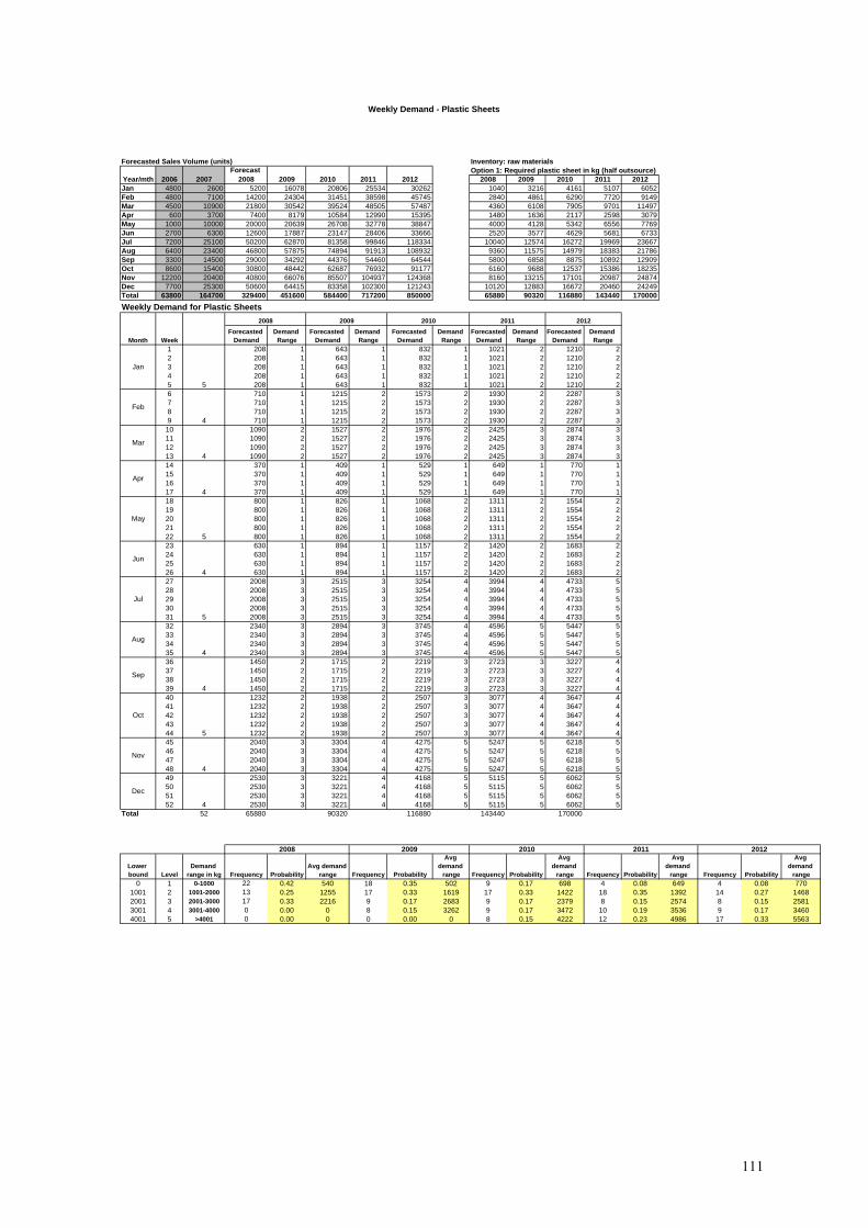
Weekly Demand - Plastic Sheets

Forecasted Sales Volume (units) Inventory: raw materialsOption 1: Required plastic sheet in kg (half outsource)

2008 2009 2010 2011 2012Jan 4800 2600 5200 16078 20806 25534 30262 1040 3216 4161 5107 6052Feb 4800 7100 14200 24304 31451 38598 45745 2840 4861 6290 7720 9149Mar 4500 10900 21800 30542 39524 48505 57487 4360 6108 7905 9701 11497Apr 600 3700 7400 8179 10584 12990 15395 1480 1636 2117 2598 3079May 1000 10000 20000 20639 26708 32778 38847 4000 4128 5342 6556 7769Jun 2700 6300 12600 17887 23147 28406 33666 2520 3577 4629 5681 6733Jul 7200 25100 50200 62870 81358 99846 118334 10040 12574 16272 19969 23667Aug 6400 23400 46800 57875 74894 91913 108932 9360 11575 14979 18383 21786Sep 3300 14500 29000 34292 44376 54460 64544 5800 6858 8875 10892 12909Oct 8600 15400 30800 48442 62687 76932 91177 6160 9688 12537 15386 18235Nov 12200 20400 40800 66076 85507 104937 124368 8160 13215 17101 20987 24874Dec 7700 25300 50600 64415 83358 102300 121243 10120 12883 16672 20460 24249Total 63800 164700 329400 451600 584400 717200 850000 65880 90320 116880 143440 170000Weekly Demand for Plastic Sheets

Forecasted Demand

Demand Range

Forecasted Demand

Demand Range

Forecasted Demand

Demand Range

Forecasted Demand

Demand Range

Forecasted Demand

Demand Range

1 208 1 643 1 832 1 1021 2 1210 22 208 1 643 1 832 1 1021 2 1210 23 208 1 643 1 832 1 1021 2 1210 24 208 1 643 1 832 1 1021 2 1210 25 208 1 643 1 832 1 1021 2 1210 26 710 1 1215 2 1573 2 1930 2 2287 37 710 1 1215 2 1573 2 1930 2 2287 38 710 1 1215 2 1573 2 1930 2 2287 39 710 1 1215 2 1573 2 1930 2 2287 3

10 1090 2 1527 2 1976 2 2425 3 2874 311 1090 2 1527 2 1976 2 2425 3 2874 312 1090 2 1527 2 1976 2 2425 3 2874 313 1090 2 1527 2 1976 2 2425 3 2874 314 370 1 409 1 529 1 649 1 770 115 370 1 409 1 529 1 649 1 770 116 370 1 409 1 529 1 649 1 770 117 370 1 409 1 529 1 649 1 770 118 800 1 826 1 1068 2 1311 2 1554 219 800 1 826 1 1068 2 1311 2 1554 220 800 1 826 1 1068 2 1311 2 1554 221 800 1 826 1 1068 2 1311 2 1554 222 800 1 826 1 1068 2 1311 2 1554 223 630 1 894 1 1157 2 1420 2 1683 224 630 1 894 1 1157 2 1420 2 1683 225 630 1 894 1 1157 2 1420 2 1683 226 630 1 894 1 1157 2 1420 2 1683 227 2008 3 2515 3 3254 4 3994 4 4733 528 2008 3 2515 3 3254 4 3994 4 4733 529 2008 3 2515 3 3254 4 3994 4 4733 530 2008 3 2515 3 3254 4 3994 4 4733 531 2008 3 2515 3 3254 4 3994 4 4733 532 2340 3 2894 3 3745 4 4596 5 5447 533 2340 3 2894 3 3745 4 4596 5 5447 534 2340 3 2894 3 3745 4 4596 5 5447 535 2340 3 2894 3 3745 4 4596 5 5447 536 1450 2 1715 2 2219 3 2723 3 3227 437 1450 2 1715 2 2219 3 2723 3 3227 438 1450 2 1715 2 2219 3 2723 3 3227 439 1450 2 1715 2 2219 3 2723 3 3227 440 1232 2 1938 2 2507 3 3077 4 3647 441 1232 2 1938 2 2507 3 3077 4 3647 442 1232 2 1938 2 2507 3 3077 4 3647 443 1232 2 1938 2 2507 3 3077 4 3647 444 1232 2 1938 2 2507 3 3077 4 3647 445 2040 3 3304 4 4275 5 5247 5 6218 546 2040 3 3304 4 4275 5 5247 5 6218 547 2040 3 3304 4 4275 5 5247 5 6218 548 2040 3 3304 4 4275 5 5247 5 6218 549 2530 3 3221 4 4168 5 5115 5 6062 550 2530 3 3221 4 4168 5 5115 5 6062 551 2530 3 3221 4 4168 5 5115 5 6062 552 2530 3 3221 4 4168 5 5115 5 6062 5

Total 52 65880 90320 116880 143440 170000

Lower bound Level

Demand range in kg Frequency Probability

Avg demand range Frequency Probability

Avg demand

range Frequency Probability

Avg demand

range Frequency Probability

Avg demand

range Frequency Probability

Avg demand

range0 1 0-1000 22 0.42 540 18 0.35 502 9 0.17 698 4 0.08 649 4 0.08 770

1001 2 1001-2000 13 0.25 1255 17 0.33 1619 17 0.33 1422 18 0.35 1392 14 0.27 14682001 3 2001-3000 17 0.33 2216 9 0.17 2683 9 0.17 2379 8 0.15 2574 8 0.15 25813001 4 3001-4000 0 0.00 0 8 0.15 3262 9 0.17 3472 10 0.19 3536 9 0.17 34604001 5 >4001 0 0.00 0 0 0.00 0 8 0.15 4222 12 0.23 4986 17 0.33 5563

2012

5

5

4

4

2010 20112009

4

4

2008

4

5

4

4

4

2012Year/mth 2006 2007Forecast

2008 2009 2010 2011

Jan

Month Week

5

Feb

Mar

Apr

May

Oct

Nov

Dec

Jun

Jul

Aug

Sep

20122008 2009 2010 2011

111

Appendix IV:

Pay-off Calculation

112

Pay-off Calculation

Planting Trays: selling price @ Baht 14/unit

Machine Labor Utilities Total Fixed Cos

410,000 360,000 360,000 1,130,000 8.99 2,050,000 Demand Revenue Demand Revenue Demand Revenue Demand Revenue

820,000 360,000 720,000 1,900,000 8.99 2,050,000 1 2008 280,000 3,920,000 330,000 4,620,000 380,000 5,320,000

1,520,000 540,000 1,020,000 3,080,000 5.60 5,550,000 2 2009 402,000 5,628,000 452,000 6,328,000 502,000 7,028,000

1,110,000 540,000 660,000 2,310,000 5.60 5,550,000 3 2010 534,000 7,476,000 584,000 8,176,000 634,000 8,876,000

1,520,000 540,000 1,020,000 3,080,000 5.60 2,050,000 4 2011 667,000 9,338,000 717,000 10,038,000 767,000 10,738,000 644,000 9,016,000

700,000 180,000 300,000 1,180,000 28.00 5 2012 800,000 11,200,000 850,000 11,900,000 900,000 12,600,000 644,000 9,016,000

Extending market: Plastic sheets: selling @ Baht 45/kgAlternative 1: Start-up with one machine

2008 2009 2010 2011 2012

Pay-off (NPV of profits)

Sales Volume

(kg) RevenueSales

Volume (Kg) Revenue773,800 1,385,020 2,046,340 2,096,440 2,096,440 6,495,944 280,000 12,600,000 480,000 21,600,000 773,800 1,385,020 3,660- 1,942,670 2,609,000 5,104,482 773,800 1,385,020 3,503,660- 3,362,800 4,480,000 4,643,380 Discount Factors523,300 1,134,520 1,795,840 2,096,440 2,096,440 5,850,406 Periods 8%523,300 1,134,520 254,160- 1,692,170 2,358,500 4,104,335 1 0.9259523,300 1,134,520 3,754,160- 2,942,800 4,060,000 3,403,289 2 0.8573272,800 884,020 1,545,340 2,096,440 2,096,440 5,204,867 3 0.7938272,800 884,020 504,660- 1,441,670 2,108,000 3,104,189 4 0.735272,800 884,020 4,004,660- 2,522,800 3,640,000 2,163,199 5 0.6806

Alternative 2: Start-up with two machines

2008 2009 2010 2011 2012

Pay-off (NPV of profits) Factor of an annuity

882,000 1,906,800 3,015,600 3,099,600 3,099,600 9,232,920 Periods 8%Expand: vacuum m/c 882,000 1,906,800 965,600 3,362,800 4,480,000 8,738,583 1 0.9259

462,000 1,486,800 2,595,600 3,099,600 3,099,600 8,150,580 2 1.7833Expand: vacuum m/c 462,000 1,486,800 545,600 2,942,800 4,060,000 7,061,691 3 2.5771

42,000 1,066,800 2,175,600 3,099,600 3,099,600 7,068,240 4 3.3121Expand: vacuum m/c 42,000 1,066,800 125,600 2,522,800 3,640,000 5,384,799 5 3.9927

3,580,000 3,580,000 3,580,000 3,580,000 3,580,000 14,293,866 6,980,000 6,980,000 6,980,000 6,980,000 6,980,000 27,869,046

Modest: 30% of cap (0.5) Large: 50% of cap (0.5)

Option 2

Modest volume

Expand vacuum m/c at year end 3Extending plastic sheet market

Large volume

High

Moderate

Low

Not expand

Not expand

Not expand

Option 1

Not Expand

Extending market

High

Variable Cost (Baht per unit)

Initial Investment

Expansion Cost

Not expandModerate

Expand: vacuum &

Vacuum m/c at year 0Expand: vacuum m/c at year end 3

Expand: vacuum & extrusion m/c at year end 3

Vacuum & Extrusion m/c at year 0

Probability of Demand LevelLow (0.3) Moderate (0.6) High (0.1)Periods (Year)

Expand: vacuum m/cExpand: vacuum &

LowNot expandExpand: vacuum m/cExpand: vacuum &

Annual Fixed Cost (Baht)

Not expandExpand: vacuum m/c

113