a feasibility study of setting up a pre-sorting system for

Masters thesis

A feasibility study of setting up a pre-sortingsystem for recyclable textiles and textile

waste in Denmark

M.B. Møller-Madsen, N. Dobler & S. Sandager

Operations and Supply Chain Management

Aalborg University

School of Engineering and ScienceOperations and Supply Chain ManagementStrandvejen 12-149000 Aalborghttp://www.tnb.aau.dk

Title:A feasibility study of setting up a pre-sorting system for recyclable textiles and textilewaste in Denmark

Project:

Masters thesis

Project period:

Spring semester 2021

Group members:

Mads Bjerregaard Møller-MadsenNina DoblerStephanie Sandager

Supervisor:

Iskra Dukovska-Popovska

Page number: 84Appendix in report: 2Appendix attached: 4Finished June 2nd 2021

The content of the report is freely available, but publication (with source reference) may only take place in

agreement with the authors.

Preface

Acknowledgements

We would like to thank Iskra Dukovska-Popovska for her supervision and guidancethroughout the duration of the project. We would furthermore like to thank Kaj Pihl fromUFF, Steen Trasborg from Trasborg, Claus Nielsen from Red Cross, Lars Wiuff Sprogøefrom DanChurchAid, Gert Pedersen from Salvation Army, Jannie Zillig from Danmission,and Kresten Thomsen from ARWOS for their cooperation in the information collectionphase of this project. Lastly, we would like to thank Nikola Kiørboe for her expertise andsupport throughout this project.

Reading guide

When referring to appendixes A.1 and A.2 it means the appendixes that are within thisreport, and when referring to attached appendixes B.1 through B.4 it describes the onesthat are attached to the report in the system where it was turned in.When a number in square brackets is used, e.g. [1], it indicates a citation of a source. Therespective information on the source can be found in the Bibliography in the end of thereport. When the citation includes a ’p.’ followed by a number within the brackets, e.g.[1,p.1], it refers to a specific PDF-page in the source where the referenced information canbe found.In this report the following abbreviations are used; DKK (Danish kroner), kg (kilogram),km (kilometer), NGO (Non-governmental organization).When a term is followed by a parenthesis, e.g. waste management company (WMC),the parenthesis informs the reader of the abbreviation of said name. This abbreviation ishereafter used for the remainder of the report.When the title of a table or figure contains the reference ’S1’, ’S2’ or ’S3’ it means thatthe table or figure displays data or information regarding the corresponding scenario. Forexample, figure 4.1 has the title ’Decision variables for MILP S1’, meaning that it displaysthe decision variables for the MILP in scenario 1.When the terms facilities and locations are used throughout the report in regards ofdetermining possible facilities and locations through the MILP, it is important to notethat this can also be one single facility or location.

Mads Bjerregaard Møller-Madsen Nina Dobler Stephanie Sandager

iii

Contents

Acknowledgements . . . . . . . . . . . . . . . . . . . . . . . . . . . . . . . . . . . iiiReading guide . . . . . . . . . . . . . . . . . . . . . . . . . . . . . . . . . . . . . . iii

Contents iv

List of Figures vii

List of Tables viii

Summary x

1 Introduction 11.1 Used textile system in Denmark . . . . . . . . . . . . . . . . . . . . . . . . . 1

Used textile system initiatives . . . . . . . . . . . . . . . . . . . . . . 51.2 Problem statement . . . . . . . . . . . . . . . . . . . . . . . . . . . . . . . . 61.3 Literature review . . . . . . . . . . . . . . . . . . . . . . . . . . . . . . . . . 6

2 Methodology 82.1 Research framework . . . . . . . . . . . . . . . . . . . . . . . . . . . . . . . 8

2.1.1 Preliminary analysis . . . . . . . . . . . . . . . . . . . . . . . . . . . 82.1.2 Scenario analysis . . . . . . . . . . . . . . . . . . . . . . . . . . . . . 102.1.3 Scenario evaluation . . . . . . . . . . . . . . . . . . . . . . . . . . . . 112.1.4 Data collection . . . . . . . . . . . . . . . . . . . . . . . . . . . . . . 122.1.5 Data validity . . . . . . . . . . . . . . . . . . . . . . . . . . . . . . . 13

3 Preliminary analysis 143.1 Required pre-sorting level . . . . . . . . . . . . . . . . . . . . . . . . . . . . 143.2 Current actors in Denmark . . . . . . . . . . . . . . . . . . . . . . . . . . . 153.3 Volume of recyclables and textile waste . . . . . . . . . . . . . . . . . . . . . 16

3.3.1 Current and future volumes . . . . . . . . . . . . . . . . . . . . . . . 19Distribution of volume within Denmark . . . . . . . . . . . . . . . . 21

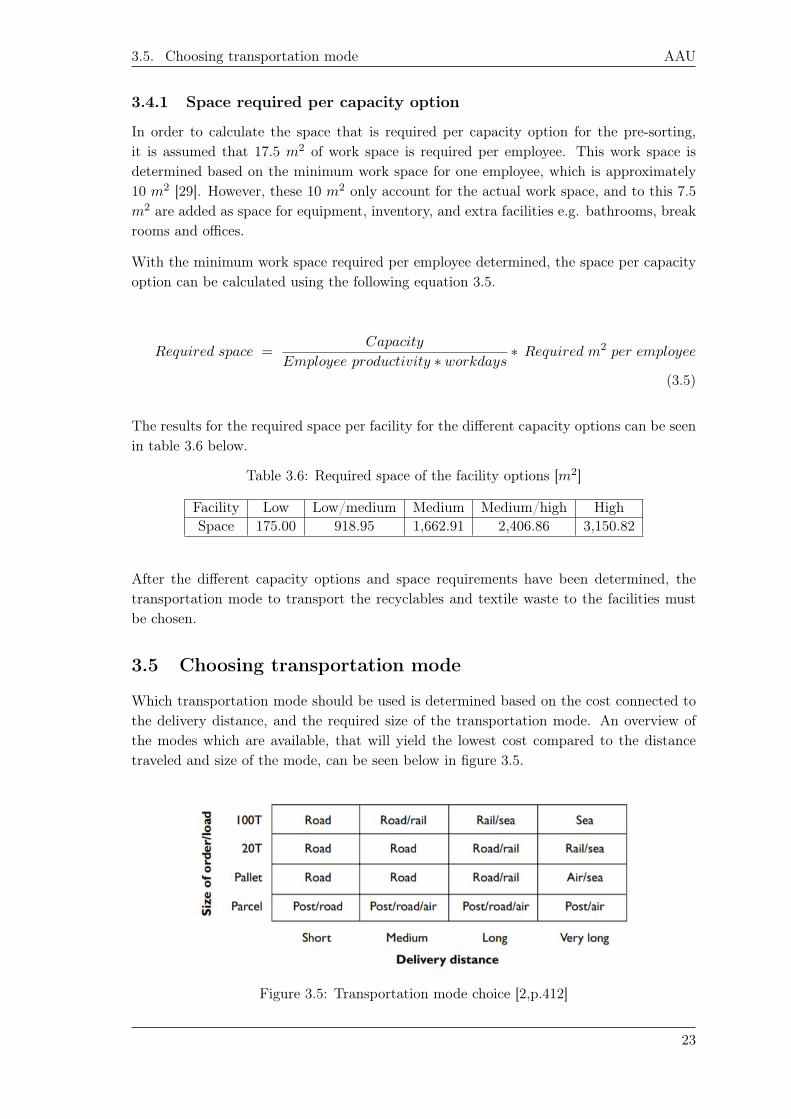
3.4 Capacity options for pre-sorting facilities . . . . . . . . . . . . . . . . . . . . 223.4.1 Space required per capacity option . . . . . . . . . . . . . . . . . . . 23

3.5 Choosing transportation mode . . . . . . . . . . . . . . . . . . . . . . . . . 233.6 Costs of the pre-sorting system . . . . . . . . . . . . . . . . . . . . . . . . . 26

3.6.1 Variable costs . . . . . . . . . . . . . . . . . . . . . . . . . . . . . . . 26Transportation cost . . . . . . . . . . . . . . . . . . . . . . . . . . . 26Employee wages . . . . . . . . . . . . . . . . . . . . . . . . . . . . . 28

3.6.2 Fixed costs . . . . . . . . . . . . . . . . . . . . . . . . . . . . . . . . 31Renting cost . . . . . . . . . . . . . . . . . . . . . . . . . . . . . . . 31Opening and expansion cost . . . . . . . . . . . . . . . . . . . . . . . 31

3.7 Sub-conclusion preliminary analysis . . . . . . . . . . . . . . . . . . . . . . . 31

iv

Contents AAU

4 Scenario 1 334.1 Current system with adjustments . . . . . . . . . . . . . . . . . . . . . . . . 334.2 Inputs to MILP . . . . . . . . . . . . . . . . . . . . . . . . . . . . . . . . . . 34

4.2.1 Variable costs . . . . . . . . . . . . . . . . . . . . . . . . . . . . . . . 35Transportation cost . . . . . . . . . . . . . . . . . . . . . . . . . . . 35Employee wages . . . . . . . . . . . . . . . . . . . . . . . . . . . . . 37

4.2.2 Fixed costs . . . . . . . . . . . . . . . . . . . . . . . . . . . . . . . . 384.3 MILP scenario 1 . . . . . . . . . . . . . . . . . . . . . . . . . . . . . . . . . 39

4.3.1 Results . . . . . . . . . . . . . . . . . . . . . . . . . . . . . . . . . . 414.4 Sub-conclusion scenario 1 . . . . . . . . . . . . . . . . . . . . . . . . . . . . 44

5 Scenario 2 455.1 New pre-sorting facilities . . . . . . . . . . . . . . . . . . . . . . . . . . . . . 455.2 Inputs to MILP . . . . . . . . . . . . . . . . . . . . . . . . . . . . . . . . . . 46

5.2.1 Variable costs . . . . . . . . . . . . . . . . . . . . . . . . . . . . . . . 465.2.2 Fixed costs . . . . . . . . . . . . . . . . . . . . . . . . . . . . . . . . 47

5.3 MILP scenario 2 . . . . . . . . . . . . . . . . . . . . . . . . . . . . . . . . . 495.3.1 Results . . . . . . . . . . . . . . . . . . . . . . . . . . . . . . . . . . 50

5.4 Sub-conclusion scenario 2 . . . . . . . . . . . . . . . . . . . . . . . . . . . . 53

6 Scenario 3 546.1 Hybrid scenario . . . . . . . . . . . . . . . . . . . . . . . . . . . . . . . . . . 546.2 Inputs to MILP . . . . . . . . . . . . . . . . . . . . . . . . . . . . . . . . . . 54

6.2.1 Variable costs . . . . . . . . . . . . . . . . . . . . . . . . . . . . . . . 556.2.2 Fixed costs . . . . . . . . . . . . . . . . . . . . . . . . . . . . . . . . 55

6.3 MILP scenario 3 . . . . . . . . . . . . . . . . . . . . . . . . . . . . . . . . . 556.3.1 Results . . . . . . . . . . . . . . . . . . . . . . . . . . . . . . . . . . 56

6.4 Sub-conclusion scenario 3 . . . . . . . . . . . . . . . . . . . . . . . . . . . . 60

7 Scenario evaluation 617.1 AHP . . . . . . . . . . . . . . . . . . . . . . . . . . . . . . . . . . . . . . . . 61

7.1.1 Determining the criteria . . . . . . . . . . . . . . . . . . . . . . . . . 62CO2 emissions . . . . . . . . . . . . . . . . . . . . . . . . . . . . . . 63Total cost . . . . . . . . . . . . . . . . . . . . . . . . . . . . . . . . . 63Excess capacity . . . . . . . . . . . . . . . . . . . . . . . . . . . . . . 64Risk . . . . . . . . . . . . . . . . . . . . . . . . . . . . . . . . . . . . 64

7.1.2 Ranking of criteria . . . . . . . . . . . . . . . . . . . . . . . . . . . . 647.1.3 Ranking of scenarios . . . . . . . . . . . . . . . . . . . . . . . . . . . 66

CO2 emissions . . . . . . . . . . . . . . . . . . . . . . . . . . . . . . 67Total cost . . . . . . . . . . . . . . . . . . . . . . . . . . . . . . . . . 67Excess capacity . . . . . . . . . . . . . . . . . . . . . . . . . . . . . . 68Risk . . . . . . . . . . . . . . . . . . . . . . . . . . . . . . . . . . . . 69

7.1.4 Assessment . . . . . . . . . . . . . . . . . . . . . . . . . . . . . . . . 707.2 Economic feasibility . . . . . . . . . . . . . . . . . . . . . . . . . . . . . . . 717.3 Barriers and benefits for pre-sorting in Denmark . . . . . . . . . . . . . . . 727.4 Sub-conclusion scenario evaluation . . . . . . . . . . . . . . . . . . . . . . . 74

v

Contents

8 Discussion 758.1 Preliminary analysis . . . . . . . . . . . . . . . . . . . . . . . . . . . . . . . 758.2 Scenario analysis . . . . . . . . . . . . . . . . . . . . . . . . . . . . . . . . . 788.3 Scenario evaluation . . . . . . . . . . . . . . . . . . . . . . . . . . . . . . . . 79

9 Conclusion 80

10 Reflection 8210.1 Further studies . . . . . . . . . . . . . . . . . . . . . . . . . . . . . . . . . . 83

Bibliography 85

A Appendix 88A.1 Appendix 1 . . . . . . . . . . . . . . . . . . . . . . . . . . . . . . . . . . . . 88A.2 Appendix 2 . . . . . . . . . . . . . . . . . . . . . . . . . . . . . . . . . . . . 89

vi

List of Figures

1.1 Waste hierarchy . . . . . . . . . . . . . . . . . . . . . . . . . . . . . . . . . . . . 21.2 Current used textile flows in Denmark . . . . . . . . . . . . . . . . . . . . . . . 31.3 Stages from collection to recycling for used textiles . . . . . . . . . . . . . . . . 4

3.1 Current locations of sorting facilities . . . . . . . . . . . . . . . . . . . . . . . . 163.2 Textile flow in Denmark in tons (2016) [1,p.30] . . . . . . . . . . . . . . . . . . 173.3 Sample size 2016 ARWOS . . . . . . . . . . . . . . . . . . . . . . . . . . . . . . 183.4 Increase in used textiles volume from 2016 - 2026 [tons] . . . . . . . . . . . . . 213.5 Transportation mode choice [2,p.412] . . . . . . . . . . . . . . . . . . . . . . . . 233.6 Tipping container truck [3] . . . . . . . . . . . . . . . . . . . . . . . . . . . . . 25

4.1 Decision variables for MILP S1 . . . . . . . . . . . . . . . . . . . . . . . . . . . 414.2 Location results for S1 . . . . . . . . . . . . . . . . . . . . . . . . . . . . . . . . 42



7.1 AHP scale by Saaty . . . . . . . . . . . . . . . . . . . . . . . . . . . . . . . . . 627.2 Criteria scoring . . . . . . . . . . . . . . . . . . . . . . . . . . . . . . . . . . . . 647.3 Standardized matrix criteria . . . . . . . . . . . . . . . . . . . . . . . . . . . . . 657.4 Ws input to the CI & CR calculations . . . . . . . . . . . . . . . . . . . . . . . 667.5 Scores per scenario for CO2 emissions . . . . . . . . . . . . . . . . . . . . . . . 677.6 Scores per scenario for total cost . . . . . . . . . . . . . . . . . . . . . . . . . . 687.7 Scores per scenario for excess capacity . . . . . . . . . . . . . . . . . . . . . . . 697.8 Scores per scenario for risk . . . . . . . . . . . . . . . . . . . . . . . . . . . . . 707.9 AHP results . . . . . . . . . . . . . . . . . . . . . . . . . . . . . . . . . . . . . . 707.10 Price development . . . . . . . . . . . . . . . . . . . . . . . . . . . . . . . . . . 72

vii

List of Tables

3.1 Collected and pre-sorted volumes of actors in Denmark . . . . . . . . . . . . . . 153.2 Used textiles collected in the US (1990-2018) . . . . . . . . . . . . . . . . . . . 193.3 Calculation of expected textile volume for pre-sorting . . . . . . . . . . . . . . . 203.4 Current volumes per region [tons] . . . . . . . . . . . . . . . . . . . . . . . . . . 223.5 Capacities of the facility options [tons] . . . . . . . . . . . . . . . . . . . . . . . 223.6 Required space of the facility options [m2] . . . . . . . . . . . . . . . . . . . . . 233.7 Average hourly wage per pre-sorter per region [DKK/hour] . . . . . . . . . . . 283.8 Average wage per pre-sorter per region [DKK/ton] . . . . . . . . . . . . . . . . 293.9 Average monthly wage per production manager per region [DKK/month][4] . . 293.10 Average wage per production manager [DKK/tons] . . . . . . . . . . . . . . . . 30

4.1 Possible facility locations S1 . . . . . . . . . . . . . . . . . . . . . . . . . . . . . 344.2 Number of trips required from each region S1 . . . . . . . . . . . . . . . . . . . 354.3 Weighted km per facility per region S1 . . . . . . . . . . . . . . . . . . . . . . . 364.4 Variable costs per facility per region S1 [DKK/ton] . . . . . . . . . . . . . . . . 384.5 Average renting cost per facility S1 [DKK/m2] . . . . . . . . . . . . . . . . . . 384.6 Fixed cost per facility per capacity option S1 [DKK/year] . . . . . . . . . . . . 394.7 Number of employees and excess capacity per facility S1 . . . . . . . . . . . . . 424.8 Cost overview S1 . . . . . . . . . . . . . . . . . . . . . . . . . . . . . . . . . . . 434.9 Future total cost S1 . . . . . . . . . . . . . . . . . . . . . . . . . . . . . . . . . 44

5.1 Possible facility locations S2 . . . . . . . . . . . . . . . . . . . . . . . . . . . . . 465.2 Weighted km per facility per region S2 . . . . . . . . . . . . . . . . . . . . . . . 475.3 Variable costs per facility per region S2 [DKK/ton] . . . . . . . . . . . . . . . . 475.4 Average renting cost per facility S2 [DKK/m2] . . . . . . . . . . . . . . . . . . 485.5 Fixed cost per facility per capacity option S2 [DKK/year] . . . . . . . . . . . . 485.6 Number of employees and excess capacity per facility S2 . . . . . . . . . . . . . 515.7 Cost overview S2 . . . . . . . . . . . . . . . . . . . . . . . . . . . . . . . . . . . 525.8 Future total cost S2 . . . . . . . . . . . . . . . . . . . . . . . . . . . . . . . . . 53

6.1 Possible facility locations S3 . . . . . . . . . . . . . . . . . . . . . . . . . . . . . 546.2 Number of employees and excess capacity per facility S3 . . . . . . . . . . . . . 586.3 Cost overview S3 . . . . . . . . . . . . . . . . . . . . . . . . . . . . . . . . . . . 586.4 Future total cost S3 . . . . . . . . . . . . . . . . . . . . . . . . . . . . . . . . . 60

7.1 Total cost of scenarios [DKK] . . . . . . . . . . . . . . . . . . . . . . . . . . . . 617.2 Possible criteria for scenario evaluation . . . . . . . . . . . . . . . . . . . . . . . 637.3 Distance [km] and kgCO2 emitted per scenario . . . . . . . . . . . . . . . . . . 677.4 Total cost per scenario [DKK] . . . . . . . . . . . . . . . . . . . . . . . . . . . . 677.5 Excess capacity per scenario [tons] . . . . . . . . . . . . . . . . . . . . . . . . . 687.6 Summary of economics . . . . . . . . . . . . . . . . . . . . . . . . . . . . . . . . 72

viii

List of Tables AAU

A.1 Pre-sorting definitions from literature . . . . . . . . . . . . . . . . . . . . . . . 88A.2 Weighted km per facility per region S3 . . . . . . . . . . . . . . . . . . . . . . . 89A.3 Variable cost per facility per region S3 [DKK/ton] . . . . . . . . . . . . . . . . 89A.4 Average renting cost per facility S3 [DKK/m2] . . . . . . . . . . . . . . . . . . 90A.5 Fixed cost per facility per capacity option S3 [DKK/year] . . . . . . . . . . . . 90

ix

Summary

Målet med dette projekt er at evaluere om det giver mening fra et økonomisk perspektiv atopstille et system der for-sortere genanvendelige- og affalds-tekstiler i Danmark. Samtidigvil der blive undersøgt hvor stor den miljømæssige påvirkning af dette system vil være.Dette bliver gjort gennem brug af metoderne Mixed Integer Linear Programming (MILP)og Analytical Hierachy Process (AHP).Grundlaget for dette projekt er lovændringer i Danmark der kræver at der indføres separatindsamling af brugte tekstiler fra den 1. januar 2022, for at skabe bæredygtighed i dennesektor. Denne indsamling bliver udført af de kommunalt ejede affaldshåndteringsfirmaer iDanmark, og det bliver antaget at denne indsamling sker gennem brug af specielle poser derkun skal indeholde genanvendelige- og affalds-tekstiler. Disse poser bliver smidt ud sammenmed pap og papir på husstandsniveau. For-sorterings niveauet er bestemt ved at undersøgehvilke krav den efterfølgende sorterings proces har. Derefter bliver de 6 største aktørerpå det danske marked identificeret for at sammenligne deres sorterings niveau med for-sorterings kravet, hvilket konkluderer at disse aktører skal foretage nogle justeringer for atkunne for-sortere. Herefter bliver inputtene til MILPerne bestemt, heraf bliver nuværendeog fremtidige mængder af genanvendelige- og affalds-tekstiler i Danmark fundet, og detbliver bestemt hvordan disse er fordelt i landet. Dernæst bliver kapacitetsniveauerne forde mulige for-sorterings faciliteter, og størrelsen på disse udregnet, samt metoden brugttil transport af disse tekstiler bestemt. Det sidste input er omkostninger af systemetsom er yderligere inddelt i variable- og faste-omkostninger. De variable omkostningerer bestemt gennem transport og lønninger for de ansatte, og de faste omkostninger erbestemt gennem leje af faciliteterne, og omkostninger ved åbning af nye eller udvidelse afeksisterende faciliteter.Tre scenarier bliver herefter analyseret ved brug af MILP, det første scenarie konkluderer attre eksisterende faciliteter skal åbnes, og resulterer i en total omkostning på 58.970.141,75DKK og 507.269,2 kgCO2 udledt. Scenarie 2 konkluderer at fire nye faciliteter skal åbnes,hvilket resulterer i en total omkostning på 57.347.348,29 DKK og 378.589 kgCO2 udledt.Scenarie 3 konkludere at tre nye faciliteter og to eksisternede skal åbnes, hvilket giver entotal omkostning på 56.671.842,11 DKK og 369.579,12 kgCO2 udledt.Til slut bliver AHP brugt til at evaluere de tre scenarier ved brug af flere kriterier endblot omkostning, disse kriterier er CO2 udslip, total omkostning, risiko, og overskydendekapacitet. Kriterierne bliver tilskrevet en score baseret på deres vigtighed når en løsningbliver evalueret, her er total omkostning det vigtigste, efterfulgt af CO2 udledning, derefteroverskydende kapacitet, og til sidst risiko. Dette resulterer i at scenarie 3 er den mestoptimale løsning af de tre scenarier. Herefter bliver muligheder for indkomst gennem salgaf genanvendelige tekstiler bestemt, og sammenlignet med omkostningerne ved at drivefor-sorterings faciliteterne. Gennem sammenligningen af dette bliver det konkluderet, atdet ikke giver mening fra et økonomisk perspektiv at oprette et for-sorterings system iDanmark men det optimale system ville have en miljømæssig påvirkning på 369.579,12kgCO2.

x

Introduction 1This chapter will give an introduction to the planned law changes regarding the wastefraction of used textiles, in the EU and in Denmark. Hereafter, a brief overview of thecurrent used textile system in Denmark will be presented, to gain an overview of theflows herein. From this, it will be described how the new used textile system is assumed tofunction after the implementation of the law changes on January 1st 2022. Next a problemstatement is proposed based on the collected information, lastly literature relevant to theproblem that was proposed is reviewed.

1.1 Used textile system in Denmark

In May of 2018 there was an amendment to the EU directive regarding waste prevention,management legislation and policy, which has a focus on circular economy within the EU. Itstates that 10 waste fractions, including used textiles, should be separately collected fromhouseholds, and thereby eliminate mixed collection. These separately collected fractionsshould be reused and/or recycled instead of being incinerated or landfilled. All used textilesfrom countries that are a member of the EU should be separately collected and sorted atthe latest by January 1st 2025. [5,p.21] From these used textiles, reusable textiles must stillbe donated directly to NGOs or other private collection companies, however, who handlesthe remaining fractions of the used textiles, which are recyclables and textile waste is yetto be determined. Therefore, the focus of this project is on recyclables and textile waste.The definitions of reuse and recycling used throughout this report are the same as thedefinitions from the EU directive from the article ’Guidance on the interpretation of keyprovisions of Directive 2008/98/EC on waste’ [6]. Reuse is defined as ’any operation bywhich products or components that are not waste are used again for the same purpose forwhich they were conceived’ [6,p.30]. And recycling is defined as ’any recovery operationby which waste materials are reprocessed into products, materials or substances whetherfor the original or other purposes. It includes the reprocessing of organic material butdoes not include energy recovery and the reprocessing into materials that are to be usedas fuels or backfilling operations’ [6,p.32]. No definition of textile waste has been foundthrough literature research and therefore it will be defined through the definitions of reuseand recycling as ’any textile that can not be reused and/or recycled and therefore ends upbeing burned or landfilled’.Following the EU directive the Danish government proposed a climate plan for Denmark,which states that the separate collection of recyclables and textile waste has to be carriedout by the municipalities from January 1st 2022. The sorting process of these must beput up for bidding where only private companies are allowed to place a bid. Thereforethe municipalities will not be allowed to perform the sorting unless no adequate bid has

1

1. Introduction

been made throughout multiple bidding rounds. This also excludes most NGOs, as theydo not pay VAT and they are therefore excluded from being able to place a bid. It isthe responsibility of the individual municipality that the regulations for treatment of usedtextiles are complied with by the winner of the bid, this also includes complying with thewaste hierarchy [7,p.7-8]. The waste hierarchy, as seen in figure 1.1, states what type ofprocess is the most preferable to the least preferable in regards to the overall environmentalimpact the process will have that it has to go through [8,p.6].Prevention is reduction of textile resource usage, and will therefore decrease the generaltextile demand and lead to less textiles being manufactured. The previous definitionof reuse and recycling is still applicable to the waste hierarchy. Recovery and Disposalare both handling textile waste, however, recovery means recovering energy throughincineration and disposal is either incineration without any energy recovery or it islandfilled. [9]

Figure 1.1: Waste hierarchy

The flows of used textiles in Denmark were mapped by Miljøstyrelsen (the environmentaldepartment) in 2016 in the article ‘Kortlægning af tekstilflow I Danmark’ [1,p.30]. Itestimated that approximately 36,000 tons of used textiles were separately collected fromhouseholds, and approximately 41,000 tons of textiles were directly incinerated in 2016 inDenmark. These incinerated textiles were collected as a part of mixed collection from smallcombustibles, bulky waste or household mixed waste, instead of being separately collected.Mixed collection is when a number of different waste fractions are collected through thesame collection method, and then incinerated.Currently, separate collection of used textiles in Denmark occurs through either bags,bins, or store collection. The collection of used textiles in bags is done in a few locationsin Denmark, for municipalities by waste management companies (WMC), these beingARWOS and AffaldPlus. The bags are disposed of as part of paper and cardboard bins ona household level. These bags are then transported to the WMCs and sorted out of theother waste fractions. Some of the bags are being opened by the WMCs in order to pick thebest quality reusable textile items for sale in their second hand shops, henceforth referredto as cherry picking. The remaining textiles are exported unsorted or partially sorted,while the sorted out waste is incinerated. The majority of NGOs have donation points,in form of bins, for used textiles at WMCs and in different cities throughout the country,and some have their own thrift stores where they also collect and sort used textiles. All

2

1.1. Used textile system in Denmark AAU

textiles that are not sold in stores, are exported, incinerated or landfilled. Trasborg iscurrently the only private actor in Denmark, who separately collects and partially sortstheir used textiles, for either export, incineration or landfill. This collection happensthrough bins located throughout Denmark. Currently NGOs and private collectors inDenmark, solely wish to receive reusable textiles as this is currently the only textile typethat is economically feasible to handle, as informed by multiple actors in the used textileindustry in Denmark. Economic feasibility is defined by Cambridge as ’the degree to whichthe economic advantages of something to be made, done, or achieved are greater than theeconomic costs’ [10], in this case it means, only the sale of reusable textile generate moreincome than handling costs required.The flows of mixed- and separate-collection can be seen in figure 1.2 below.

Figure 1.2: Current used textile flows in Denmark

From January 1st 2022, used textiles should no longer be found in the mixed collection.Therefore, this project will be based on the assumption that all used textiles are collectedthrough a separate collection system, and that reusable textile are collected by NGOs orTrasborg. For the separate collection method for recyclables and textiles waste it wasinformed by Nikola Kiørboe, a used textile, circular economy and waste expert, that thebag collection was proposed to the Environmental Department to be implemented nationwide. The proposal is currently being reviewed, and a final decision on changes is expectedsometime in 2021. This report will work with the assumption that this separate collection

3

1. Introduction

method for recyclables and textile waste is approved and implemented. Both of these as-sumptions are made as this project aims to aid the decision making regarding the optionsof handling recyclables and textile waste after the separate collection.

The following figure 1.3 shows the steps connected to the handling of recyclables andtextile waste after separate collection. Before the used textiles can be recycled, theymust be sorted. When handling recyclables and textile waste there are two levels thatare commonly used, pre-sorting and sorting. Pre-sorting is the initial step of dividingcollected used textiles into categories that are required by the sorting facilities in order totake in these textiles for further processing, and remove textile waste. There is currentlyonly one actor in Denmark who pre-sorts a fraction of their collected textiles, this beingTrasborg. The pre-sorting is done manually, as currently no technology exists to performit automated. The third stage of sorting is the process of further dividing the pre-sortedtextiles into different fiber compositions depending on the requirement of the recyclingprocess. This is most commonly done by machine at automated sorting facilities, howeverthere are currently no actors in Denmark who perform this process. The last stage ofrecycling the used textiles is handled by recycling facilities, there are currently no facilitiesthat are operating in Denmark.

Figure 1.3: Stages from collection to recycling for used textiles

As previously described, it is assumed for this report that the method and responsibilityof separate collection of recyclables and textile waste is determined. The placement of re-sponsibility for the pre-sorting of used textiles has not yet been determined, which must bedone before determining who has the responsibility of the textile sorting stage. Therefore,this report will focus on determining who will perform the pre-sorting of recyclables andtextile waste in Denmark.

Currently, all recyclables and textile waste from Denmark that are not incinerated aresold and exported for pre-sorting or sale. In order to increase sustainability of the usedtextile system this pre-sorting should be kept within Denmark. This pre-sorting will alsogive the possibility to recycle these textiles instead of incinerating them, thereby followingthe waste hierarchy and increasing sustainability further. Sustainability is defined as ’Theproperty of being environmentally sustainable; the degree to which a process or enterpriseis able to be maintained or continued while avoiding the long-term depletion of natural

4

1.1. Used textile system in Denmark AAU

resources’ [11]. In regards to the used textile system, sustainability of the system meansthat it must be a long term solution, and not a quick fix of the current issue, while notexhausting natural resources. Keeping pre-sorting within Denmark would decrease thetransportation, and recycling would decrease CO2 emissions compared to incineration,and thereby the negative environmental impact. Additionally, keeping the pre-sorting ofused textiles within Denmark can, according to a Swedish feasibility study, create jobs,which is a surplus to increasing sustainability [12,p.18]. No research has been done tofind a solution to keep the pre-sorting process of recyclables and textile waste withinDenmark or who is responsible for it. This report aims to fill this gap in the literatureby determining if an economically feasible and sustainable solution is possible in Denmark.

Even though no research has been done regarding a solution for the pre-sorting in Denmark.There are initiatives regarding used textiles that have been started in other Nordiccountries, which will be described in the following.

Used textile system initiatives

In order to increase the sustainability of the used textile industry, several initiativeshave been started by different organizations and actors over the past years. Some ofthese initiatives are currently active whereas some have been terminated before finishing.One of these initiatives is the "Nordic textile reuse and recycling commitment" startedby the Nordic Council of Ministers, which aims to decrease the negative environmentalimpact by increasing reuse and recycling of Nordic textiles, through collecting, sharingand establishing best practices. [13,p.9] Currently there is no system operator who iswilling to take on this project, and therefore it has been on hold since 2017. Some ofthe individual Nordic countries have current national projects, for instance an automatedsorting facility in Sweden (SIPTex) [14] and a semi-automated facility in Finland (LSJH)[15,p.64].Another initiative is the SATIN project, which differs from the national projects as it hasa focus on the collaboration between the Nordic countries, in order to achieve advantagesby sharing resources and infrastructure. [16,p.1-2] The acronym SATIN is derived fromthe title of the research project, which is "TowardS A susTainable cIrcular system oftextiles in the Nordic region". The overall goal of the SATIN project is improvement ofthe used textile system in the Nordic region moving towards a sustainable and circular usedtextile system. Its focus is therefore put on the mapping and evaluation of the currentused textile system, and the development of cost-efficient collection solutions for increasedcollection rates. Furthermore, a circular network solution for the Nordic region should bedesigned to handle the increasing volumes of collected used textiles. They are investigatingpossibilities for shared network resources and centralized infrastructure between the Nordiccountries in order to create a shared sustainable and circular used textile system. [16,p.1]Therefore, researchers from these countries collaborate with actors from different stagesof the textile circular system, for example production, collection, reuse and recycling oftextiles. In addition, specialists in supply chain management and simulation are takingpart in the SATIN project. [16,p.7] This project is written as contribution to the SATINproject, and it is solely focused on the Danish pre-sorting system.Based on the presented information, the following problem statement is developed in order

5

1. Introduction

to guide the analysis.

1.2 Problem statement

Is it possible to design an economically feasible pre-sorting system with one or morefacilities in Denmark and how large will the environmental impact be?

The following section will describe literature that is relevant for the problem statement,and through this methods that will be applied to answer the problem statement.

1.3 Literature review

The study of feasibility of setting up a sorting facility for used textiles is not a new field.Carlson et al. (2019) evaluate the feasibility of sorting textiles in Sweden [12,p.3], andthey apply a financial feasibility analysis by calculating an estimated cost and estimatedincome per kilogram of sorted textiles. The study concludes that setting up a nationalsorting facility in Sweden is not financially feasible, as the estimated cost are higher thanthe estimated income [12,p.26]. In addition, different risk categories are suggested for theassessment of the feasibility of a sorting facility. No feasibility study has been carriedout for the pre-sorting of used textiles in Denmark, however, the flows of used textilesin Denmark have been mapped by Watson et al. (2018), who determine the inputs andoutputs of textiles to and from households, and identify the specific flows [1,p.30]. Thecurrent main used textile actors and the volumes of used textile these actors handle havebeen identified by Watson et al. (2014) [17,p.33]. Even though the field of used textileshas been studied, it has yet to be as thoroughly studied as other waste fractions. It alsodoes not have a reverse logistic system implemented like other waste fractions in Denmark,such as plastic and cardboard.

Bing et al. (2012) investigate how to provide decision support for the flow of householdplastic waste in the Netherlands by applying reverse logistics network design [18,p.1]. Theydeveloped scenarios that vary regarding the collection method and what type of plasticis collected [18,p.7-8]. To design the specific networks of the scenarios, the Mixed IntegerLinear Programming (MILP) method is applied, with the goal of minimizing transportationcost and environmental impact [18,p.9-10]. In order to account for the environmentalimpact in the MILP, the amount of CO2 emitted is converted into environmental cost oftransporting plastic. To evaluate the environmental impact of the scenarios, the actualamount of CO2 emissions is determined per scenario. The scenarios are then evaluatedbased on which has the lowest total cost of transportation and environmental impact.Alshamsi and Diabat (2015) also apply MILP [19,p.1] by formulating a model that aids indecision making when designing the reverse logistic network for consumer products. Thisparticular model has the goal of maximizing the profit based on investment [19,p.3]. Theresults of the model aid in the decision making based on the cost of the different scenarioswith the goal to maximize the profit when implementing the reverse logistic network.

When analysing scenarios, multiple criteria might be important for the evaluation, howevernot equally so, and therefore the relative importance of these must be evaluated. To do soa Multi-Criteria Decision Analysis (MCDA) can be applied. Furthermore, when applying

6

1.3. Literature review AAU

MCDA the overall performance of different scenarios can be determined, based on thesecriteria. There are a number of different MCDA methods that can be applied and thesuitability of these will vary depending on the specific use case [20,p.2].

Challcharoenwattana and Pharino (2016) apply Analytical Hierarchy Process (AHP),which is a form of MCDA, to evaluate different recycling practices for municipal solidwaste in Thailand and determine the optimal one regarding the ability to reduce cost,and willingness to recycle [21,p.1]. Milutinovic et al. (2017) set up scenarios for wastemanagement in Nis, Serbia, and determine which is the best in terms of having the leastnegative environmental impact. Like Bing et al. (2012), also here the environmental impactis measured in CO2 emissions, however further factors are included in this analysis likeheavy metals and NH3 emissions from biological processes. These scenarios are evaluatedusing a combination of Life-Cycle Assessment (LCA) and AHP. LCA is used to determinethe environmental impact of the developed scenarios, called indicators, and AHP is usedto evaluate and rank the scenarios according to the indicators. [22]

7

Methodology 2This chapter will describe how the analytical methods that were identified through theliterature review will be adapted and applied to this project along with other methodsdeveloped through knowledge from courses to answer the problem statement. It will furtherbe described how the data was collected to conduct the research. Furthermore, the validityof the collected data will be evaluated.

2.1 Research framework

This section will describe the research framework of this project, meaning the theoreticalplan for how the analysis will be conducted.It was found that scenario analysis was used multiple times throughout literature indifferent fields to analyse different possible solutions for a problem. This is found suitablefor the analysis of the used textile industry, as the pre-sorting of recyclables and textilewaste in Denmark can be performed in a number of locations with varying capacities.Therefore, for the analysis of the pre-sorting possibilities in Denmark, the approach ofscenario study will be used. Through the literature review, MILP was identified as acommonly used analytical method to determine the optimal solution of many possiblecombinations, with the goal of cost minimization or profit maximization. This is found tobe a suitable analytical method to analyse the cost of pre-sorting in Denmark, as finding thesolution with the minimum total cost will increase the likelihood of it being economicallyfeasibility.Furthermore, it was determined through the literature review that MCDA methods canbe applied for evaluating identified scenarios performance by using multiple criteria. Thisis a suitable method to apply as the MILPs only has a focus on the criteria of cost, byminimizing the total cost of the scenarios, and considering different criteria might yield adifferent optimal solution.The research framework for the analysis is below divided into 3 parts; preliminary analysis,scenario analysis and scenario evaluation, in which the applied analyses and used data willbe described.

2.1.1 Preliminary analysis

Before analysing the scenarios the current used textile system must firstly be adequatelydescribed which will be done in the preliminary analysis. This leads to identifying anddescribing the shared inputs of the scenarios.The level of required pre-sorting at any pre-sorting facility must be determined, as this willhave an impact on all of the scenarios because they all have to comply with it. The current

8

2.1. Research framework AAU

used textile system in Denmark will be analysed to identify the actors who are currentlyhandling textiles in Denmark, as they could potentially part take on the pre-sorting ofrecyclables and textile waste in the future, and thereby be a part of the scenarios of thisreport. The volumes of recyclables and textile waste that are currently and expected toin the future be in Denmark, must be determined to find the volumes there must be pre-sorted. Hereafter, the distribution within Denmark of these must be determined, in orderto account for population distribution in Denmark when determining the transportation.Possible transportation modes will be analysed in order to identify the most suitable for theload and to decrease the cost of transportation. lastly, the costs connected to the differentscenarios of pre-sorting in Denmark are investigated, in order to evaluate the economicfeasibility and it will be determined how the environmental impact will be measured.

Based on this, the following 5 questions are proposed, which will guide the preliminaryanalysis.

1. What level of pre-sorting is required?2. Who are the current actors in the Danish used textile system and can they pre-sort

recyclables and textile waste?3. What is the current and expected future volume of Danish recyclables and textile

waste?4. How is the volume distributed within Denmark?5. What transportation mode is most suitable for the transport of recyclables and textile

waste?6. What costs are associated with having pre-sorting in Denmark and how is the

environmental impact measured?

The level of pre-sorting will be determined through the requirements for the textiles ofthe following sorting process. This will be done by collecting literature and conductinginterviews with possible sorting actors on the requirements of the sorting facilities and onthe quantity of recyclables they can receive.

Through the literature review it was found that the current main used textile actors willbe identified by Watson et al. (2014) [17,p.33], these 6 actors will be used throughout thisreport. Furthermore, interviews will be conducted with these identified actors to obtainknowledge on their current sorting level.

The overall volumes of recyclables and textile waste in Denmark are currently not mappedyearly, therefore the current volume of 2021 and expected future volumes can not be foundin literature. To determine these volumes, historical data is used and to this a yearlyaverage change in the collected used textiles must be applied. The historical data will befound in the report by Miljøstyrelsen (2018) [1,p.30], which documents the 2016 textileflows and volumes in Denmark divided by collection method and quality category. Andthe average yearly expected change in collected recyclables and textile waste will be foundand applied to the historical data to find the future volume.

The volume distribution within Denmark will be determined by finding the recyclablesand textile waste generated per capita. To do so it requires data on the population ofthe Danish municipalities, which will be found through the Danish statistics database onmunicipal population [23]. Furthermore, the total volume of recyclables and textile waste

9

2. Methodology

will be used as found through the previous question. This will further be divided intototal volume per WMC by identifying what WMC services which municipalities throughresearch on their websites.

To determine the most suitable transportation mode for used textiles within Denmark,the assumed average transportation distance and average load will be applied in a decisionmatrix of transportation mode choices presented by Baker et al. (2014) [2,p.412]. Thesize of the mode will then be decided based on a comparison of the required and availablesizes, where the closest to the requirement will be chosen as it will yield the lowest cost.

When investigating different cost aspects associated to pre-sorting in Denmark, it will bedivided into variable and fixed cost. The variable cost consists of transportation cost andemployee wages, as these vary depending on the volume of recyclables and textile wastethat is pre-sorted. The transportation cost is further divided into environmental and fuelcost, for the environmental cost the same approach as used by Bing et al. (2012) [18,p.12] isapplied to convert the CO2 emitted into monetary value, in order to take the environmen-tal impact of a scenario into account in the MILP. Employee wages will be found throughliterature research on different employee wages in different regions of Denmark. The fixedcosts consist of the renting cost for the potential facilities and the cost of expanding acurrent or opening a new facility, as this cost does not vary depending on the volumeof textiles pre-sorted. Inputs to these cost calculations will be found through literatureresearch and interviews. Lastly the environmental impact will be measured by finding theactual amount of CO2 emitted per scenario, as it was done by Bing et al. (2012) [18,p.17].

2.1.2 Scenario analysis

In order to analyse possible solutions for the pre-sorting of recyclables and textile waste inDenmark, different scenarios must be developed as it was found through literature review.The information determined throughout the preliminary analysis will be used in additionto information found through interviews with experts in the used textile field, to set updifferent scenarios for the pre-sorting based on who performs it and where it takes place.The goal of this is to make it possible to find the optimal solution for the individualscenarios based on total cost.Based on the current system, NGOs are not allowed to place a bid to perform the pre-sorting for the municipalities. However, if they partially privatize their organization andstart paying VAT, they will be allowed to make a bid. The first scenario will thereforedetermine which of the NGOs are willing to make adjustments to be allowed to pre-sortrecyclables and textile waste. Scenario 2 will have focus on setting up new pre-sortingfacilities in Denmark, to give the MILP more facility location choices, which could decreasethe total cost of the pre-sorting system. The third scenario will include both the currentand new facility locations determined through scenario 1 and 2, and thereby create a hybridof the two, to analyse if this will decrease the total cost. A listing of these three scenarioscan be seen below.

• Current system with adjustments (Scenario 1)• New pre-sorting facilities (Scenario 2)• Hybrid scenario (Scenario 3)

10


For the scenario analysis, the following questions are defined to aid the analysis. Themethods applied to answer them are described based on what was identified in the literaturereview.

7. What are possible locations for pre-sorting facilities?8. What are the optimal locations and capacities for pre-sorting facilities and what is

the total cost of this?9. What is the excess capacity?10. How much CO2 is emitted?

When determining possible pre-sorting facility locations, different approaches will be takenfor the different scenarios. For the first scenario, interviews will be conducted with therelevant actors in the field, to determine if they have any interest in making adjustmentsto their business. The possible pre-sorting facility locations will be based on actors’interests in making the required adjustments. The possible locations for scenario 2 will bedetermined based on the population centers within the regions of Denmark. For scenario3 the possible locations will be the combination of the locations were identified in scenario1 and 2.

The fixed- and variable-costs of the possible pre-sorting facilities will be used as an inputto the MILP, to determine what the optimal locations and capacities for the pre-sortingfacilities are. The MILP has the goal to minimize the total cost of the pre-sorting inorder to increase its likelihood of economic feasibility. The MILP is formulated throughan objective function which calculates the total cost of a scenario. Thereby the MILPminimizes the total cost by changing specified decision variables in order to comply witha set of predetermined constraints. This means that the MILP compares all possiblecombinations within the limits set by the constraints for a scenario, to find the optimalone for the objective function. The result of the objective function will be the minimumcost of the optimal solution. This will be executed using Excel software, in an add-in calledsolver, this add-in has a limited capacity of 200 for the amount of variables it can include.

Through the constraints of the MILP, excess capacity will be enforced by setting aminimum capacity limit, the amount of excess capacity varies depending on what locationsthe scenarios choose to open and at what sizes. This constraint will be set to ensure thatthe capacity of the facilities will be able to pre-sort future volumes.

To determine how much CO2 is emitted from the scenarios, the environmental costcalculation used by Bing et al. (2012) [18,p.12] which was introduced in the literaturereview, is converted to find the CO2 emitted. However, from the environmental costformula the price per ton of CO2 emitted is removed as the emission is needed and notthe price of it.

2.1.3 Scenario evaluation

As the third part of the analysis, the scenarios will be evaluated, which is necessary todetermine which of the possible scenarios is the most optimal on other criteria than solelycost. For this evaluation, a MCDA method is applied as introduced in the literature review.Through literature it was found that AHP is a commonly used MCDA method, e.g. byChallcharoenwattana and Pharino (2016) [21,p.1] who apply it in the waste management

11

2. Methodology

industry. The AHP method also accounts for the consistency of its inputs [24,p.1], and forthese reasons it is found suitable and will be applied for this analysis. The AHP method canbe summarized in four steps. In the first step, relevant criteria will be determined throughinterviews with relevant actors and experts in the field of used textiles. Furthermore,literature will be reviewed to support these criteria and possibly identify new ones relevantto this project. In the second step the relative importance of the identified criteria willbe determined using a pairwise comparison, which requires input from experts. This willresult in a ranking of the criteria based on their relative importance. Thereafter, thedifferent scenarios will be ranked based on their performance for each of the criteria inpairwise comparisons. In the last step an assessment will be made using the relativeweight of the criteria and the rankings of the scenarios. This step will conclude which ofthe analysed scenarios scores the best. Throughout these steps a consistency ratio (CR)will be calculated, which evaluates the consistency of the input information.After determining the most optimal scenario based on the chosen criteria, it must bedetermined if this scenario is economically feasible, and lastly barriers and benefits thereare associated will be identified and described. Based on this the following questionsare posed and the required methods to answer them are described using information andmethods from the literature review.

11. What criteria are most suitable for evaluation of the scenarios?12. How are these criteria ranked in terms of importance?13. Which scenario scores the best using these criteria?14. Is the optimal scenario economically feasible?15. What are barriers and benefits associated with the optimal scenario?

To use the AHP for the scenarios, different criteria must be identified and ranked by theirrelative importance. This is done through interviews with an expert in the field to ensurethat the inputs and importance is correlating with how it actually is within the field.Through the AHP a single scenario will be determined as being the best, however thisscenario will not necessarily be economically feasible. This will therefore be evaluated bycomparing the total cost of the system to the potential income generated through sale ofrecyclables, which will lead to a conclusion on whether the scenario is economically feasibleor not. The evaluation will conclude by summarizing the results of the optimal scenarioby highlighting the barriers and benefits that the scenario will bring.

After describing the analytical methods required to answer the problem statementthroughout the research framework, the following subsections will describe the datacollection and validity for this project.

2.1.4 Data collection

The data collection of this report is conducted using the following methods: literatureresearch, interviews and secondary data collection.

If the required information is publicly available, it is collected through literature researchor secondary data collection like Science Direct. Both quantitative and qualitative datawas collected by reviewing different literature, such as reports on the used textile systemin Denmark and its flows and volumes as described in the Danish report ’Kortlægning af

12


tekstilflows i Danmark’ by Miljøstyrelsen [1,p.30]. If the data is not publicly available thenit is necessary to contact the actors or experts in the fields and conduct interviews, thesewere held with different actors within the textile industry, such as Kaj Pihl of UFF andSteen Trasborg who is CEO of Trasborg. Some of these interviews were held throughMicrosoft Teams, using the semi-structured format, which means that questions wereprepared in advance but it was possible to ask additional questions that might arise duringthe interview. The remaining were structured interviews and conducted through e-mails,where questions were formulated and sent. Through the interviews both quantitative andqualitative data was collected. An example of qualitative data collected is information onwhether the current actors are interested in making adjustments to their business to pre-sort recyclables and textile waste. Quantitative data for example the employee productivitywhen pre-sorting used textiles.

2.1.5 Data validity

Assessing the validity of the data used for the project is a critical step, as using invaliddata will lead to the outcome of the analysis being invalid, meaning it will be unusable. Inorder to validate the collected data there has to be identified potential outliers and errors,and the source of the data has to be evaluated as well. If the data contains a substantialamount of errors, the validity of the used data should be questioned. This could lead todismissing the data, and thereby new data would have to be collected and validated. Thedata validation process varies depending on whether the data is quantitative or qualitative.

Validating quantitative data is done by identifying errors like outliers or missing values,meaning notable deviates from the collected data. Here quantitative outliers were found inthe yearly used textile generation of Denmark [25]. The data point were inconsistent withinformation received from actors in the field, and the source was therefore excluded as usingit would lead to an invalid result. Another outlier was identified in the Danish mappingof used textile flows, here a figure published in two different languages, from the samedepartment has two different volume of used textile for the same flow. It is assumed thatthere was a typing error, and therefore the source that is deemed valid had to be chosen.As the original and published source is the Danish report, therefore, this is assumed tocontain the correct number, and the quantity from this source is used throughout thereport.

When evaluating the validity of qualitative data, the source of the data and its credibilitymust be assessed. A source is deemed credible and therefore the retrieved data is deemedvalid when the source is experienced in the field. An experienced source is for exampleDanish authorities, or experts in the field with years of experience. Through this reportthe Danish waste expert Nikola Kiørboe was consulted, and her information was deemedvalid as she has years of experience in the waste and used textile industry.

Where possible, used data has been validated through a data validation process and theresults of this report are therefore deemed valid.

13

Preliminary analysis 3This chapter will describe the inputs that are shared between the scenarios MILPs. Thisis done by firstly determining the level to which the used textiles have to be pre-sorted to.This leads to an introduction of the current actors in the Danish used textile system, and adetermination of whether they are capable of pre-sorting to the specified level. Thereafterthe volume required to be pre-sorted is determined per region, here including recyclablesand textile waste. Next the capacity options for a pre-sorting facility is determined, aswell as the space required for these facility options. Thereafter the transportation modeand size is chosen based on which will be least costly and closest to the amount of usedtextiles there on average has to be transported weekly. This leads to calculating the cost ofpre-sorting textiles which is determined using inputs in the form of variable- and fixed-costfactors.

3.1 Required pre-sorting level

The pre-sorting of used textiles can be done to different levels of detail, depending on therequirements of the following processes the pre-sorted textiles are to go through. Theserequirements have to be determined, because they have to be achieved during pre-sortingin order to get the textiles further sorted in the next step. Automated sorting facilitiesfurther sort the pre-sorted textiles in the next step, and therefore they set the required levelof pre-sorting for them to take in the recyclables and textile waste. Their requirementsare determined in the following.Currently, there are 2 automated sorting facilities in the Nordics, one is located in thesouth-west of Finland, and it is operated by the public waste management operatorLounais-Suomen Jätehuolto Oy (LSJH). And one is in the south of Sweden is called SIPTex,which stands for Swedish Innovation Platform for Textile sorting, and it is operated bythe municipal waste management company Sysav.The required level of pre-sorting is defined by the requirements of the individual automatedsorting facilities, the definitions of these requirements, whom they are defined by and inwhat literature can be seen in appendix A.1. In order to determine, which of the 2 sortingfacilities will sort Danish recyclables, their free capacities must be looked at. The Finishsorting facility LSJH informed, that the capacity is currently full. The Swedish facilitySIPTex has a total sorting capacity of 24,000 tons per year, and they are willing to receiveinternational feed-stock, if it fits their business operations. Because SIPTex is the onlyautomated sorting facility in the Nordics that can receive volumes from Denmark, it isassumed that the pre-sorted textiles will be sent here. Due to this, their requirement forpre-sorting will be used throughout this report. This being ’accepting pre-sorted recyclingfractions from manual sorting’, this results in pre-sorting in Denmark having to divide into

14

3.2. Current actors in Denmark AAU

three categories. These categories are; textile waste, which will be incinerated or landfilledin Denmark, reusable textiles, will be given back to the NGOs and recyclable textiles,which will be sent for further sorting at SIPTex.

3.2 Current actors in Denmark

In order to gain a more detailed overview of the used textile system in Denmark, the actorswithin it have to be determined. Watson et al (2014) identifies the following 6 actors, basedon the collected volume of used textiles per year, as the main actors who separately collectsused textiles in Denmark; Trasborg, Red Cross (Røde Kors), Salvation Army (FrelsensHær), UFF, DanChurch Social (Kirkens Korshær), and Danmission [17,p.33]. These 6actors are responsible for the separate collection of approximately 60% of the Danish usedtextiles. The remaining 40% are collected by various small organizations, meaning thateach of them is responsible for only a small share of Danish used textiles. Therefore, the6 identified main collectors will be used for the further analysis.All 6 actors separately collect used textiles trough bins and shops, however the sortingprocesses differ between the organizations. None of the actors sort the entirety of theircollected volume, but export parts of it unsorted to customers in Europe or in otherlocations around the world. The remaining fraction of the collected used textiles is sortedwithin Denmark at different levels depending on the organization, which in the table belowis referred to as handled. An overview of the identified actors and their total volume ofcollected- and handled-textiles can be seen below in table 3.1.

Table 3.1: Collected and pre-sorted volumes of actors in Denmark

Actor (year) Collected textiles [tons] Handled [tons]Trasborg (2014) 5,700 [26,p.38] 1,492 [26,p.38]Red Cross (2019) 8,319 5,343

Salvation Army (2014) 5,750 [26,p.38] 2,012 [26,p.38]UFF (2014) 1,467 [26,p.38] N/A

Danmission (2014) 1,000 [17,p.33] xDanChurch Social (2014) 5,000 [17,p.33] x

As previously described, Trasborg is the only actor in Denmark who pre-sorts a fraction oftheir collected used textiles. Trasborg has 1 sorting facility in Taastrup (E) in the regionof Hovedstaden, where currently 10 employees handle the collected used textiles. Theremaining 5 actors cherry pick the best quality textiles from what they collect. Red Crosshas 2 sorting facilities, one in Køge (D) in the region of Sjælland and one in Horsens (A)in the region of Midtjylland , where the collected textiles are cherry picked. These cherrypicked textiles are further sorted into categories for sales in the shop. The volumes as seenin the table above were informed by Claus Nielsen, who is the section leader of the reusecenters of Red Cross. Salvation Army operates 2 sorting facilities, one in Hvidovre (F)in the region of Hovedstaden and one in Kolding (B) in the region of Syddanmark wherethe collected textiles are cherry picked. Danmission operates a sorting facility in Vejle (C)in the region of Syddanmark, where a part of the collected textiles are cherry picked, butthe volumes are unknown which is therefore noted as x in the table. UFF does not havea sorting facility in Denmark, meaning that none of their collected volume is handled in

15

3. Preliminary analysis

Denmark but that all their collected used textiles are exported, which is therefore notedas N/A in the table. DanChurch Social does also not have a sorting facility in Denmark,but cherry picks part of their collected used textiles in their shops, the volumes of this areunknown and is therefore noted as x in the table. There is no information available on thenumber of sorting employees from actors besides Trasborg. The locations of the sortingfacilities can be seen in the following figure 3.1, where the letters A-F correspond with thecities as described above.

Figure 3.1: Current locations of sorting facilities

The current actors in the Danish used textile system with their current capacities can atthe moment not handle the entire volume of textiles they collect. Furthermore, majorityof the actors do not have a pre-sorting process, but they cherry pick. Because pre-sortingis a more detailed process than cherry picking it will require more time or more resourcesper ton handled, and it can therefore be assumed that the current used textile system willnot be able to pre-sort the recyclables and textile waste.

After the current main actors in the used textile system are identified, the next step isto determine the volumes of recyclables and textile waste that have to be handled by thepre-sorting facilities in the new system.

3.3 Volume of recyclables and textile waste

To determine the quantity of used textiles there must be pre-sorted, the quantities ofrecyclables and textile waste must be determined. These quantities are determined usingdata from the report by the Danish environmental department from 2016, which contains

16

3.3. Volume of recyclables and textile waste AAU

ratios for specific flows of used textiles [1,p.30]. This is the most recent published reporton Danish used textile quantities, and is therefore applied for this analysis. The followingfigure 3.2 shows the overview of textile flow from this report.

Figure 3.2: Textile flow in Denmark in tons (2016) [1,p.30]

In figure 3.2 above, ratios of different used textile quality levels can be found, which showsthat from separate collection 19% of exported textiles are recycled [1,p.30]. These ratiosare multiplied with the total volume of that specific flow of separate collection, whichis 21,840 tons, and the amount of recyclables and textile waste is thereby determined.Additionally, the flow from separate collection to recycling in Denmark must be added,which is 320 tons, as these will also be pre-sorted in Denmark.Furthermore, the amount of recyclables and textile waste from mixed collection must bedetermined. Here the report states that from the incinerated textiles approximately 23%are reusable and 26% are recyclable, and an additional 37% of textiles could be recycledin the future [1,p.5]. For this report it is assumed that the additional 37% of textileswhich can be recycled in the future must also be handled by the pre-sorting facilities.These 37% are included as they no matter what will go through the pre-sorting, if theycannot be recycled they will end up as textile waste instead. It is however throughout thereport assumes that they are recyclables. Therefore, a total of 63% of recyclables will bemultiplied with the total combined volume of incoming textiles to incineration, which is39,900 [1,p.5]. This leads to the following calculation of the total quantity of recyclables,that can be seen in the equation 3.1 below.

21, 840 tons ∗ 19% + 320 tons + 39, 900 tons ∗ 63% = 29, 606.60 tons (3.1)

As seen in the equation above the total amount of recyclables there must be pre-sorted in

17


Denmark is 29,606.60 tons.The next step is to determine the quantity of textile waste and add this to the quantity ofrecyclables, as this also will be pre-sorted with the recyclables. From separate collection11% are either landfilled or incinerated [1,p.30] of the total 21,840 tons, the volume of39,900 tons from mixed collection to incineration contains 14% waste [1,p.5], and there isa last flow of textile waste from separate collection to incineration, which is 2,230 tons.This leads to the calculation 3.2 below, using these ratios and quantities.

21, 840 tons ∗ 11% + 39, 900 tons ∗ 14% + 2, 230 tons = 10, 218.40 tons (3.2)

From equation 3.2 it can be concluded that a total quantity of 10,218.40 tons of textilewaste must be pre-sorted. The sum of the two calculated volumes is now determined,29, 606.60 tons + 10, 218.40 tons = 39, 825 tons, and thereby a total of 39,825 tons ofrecyclables and textile waste must be pre-sorted.

Additionally to the recyclables and textile waste, some reusable textiles will most likelybe put in the bag, because of either user error or from wrong judgement regarding qualityof the used textiles. From the WMC ARWOS, who is responsible for the bag collectionof used textiles in the municipalities Aabenraa and Padborg, it was informed that onaverage 11% of the bags content are reusable textiles. This information was found througha test sample made in 2016, and the daily operations leader estimates that this number isstill accurate representation of the current ratio. The division between the quality of thecollected textiles can be seen in figure 3.3 below.

Figure 3.3: Sample size 2016 ARWOS

As it is known that approximately 11% of what is collected through bags are reusabletextiles, this must be added to the 39,825 tons of recyclables and textile waste. Fromequation 3.3 below, it can be seen that this results in 44,206 tons of textiles in total thatmust be pre-sorted.

39, 825 tons ∗ 111% = 44, 206 tons (3.3)

18


This means, that during the pre-sorting process these 4,381 tons of reusable textiles haveto be sorted out during the pre-sorting along with the 10,218.40 tons of textile waste.

As the data used to calculate this total volume is from 2016, the current volume has to bedetermined by considering the yearly change in used textiles in Denmark. Furthermore, inorder to ensure that the new used textile system will be able to cope with future volumes,this yearly change must then be applied to the current volume to determine the futurevolumes.

3.3.1 Current and future volumes

The expected yearly increase of used textiles is determined using historical data on thequantities of used textiles. Data on textile collection in Denmark is limited as seen inEurostats’ report on the historical quantity of used textiles collected in Denmark [25].Here Eurostat reported that 1 ton of used textile was collected in 2004, which increased to26,854 tons in 2018. Furthermore the yearly increase between 2004 and 2018 is nonlinear,as it varies from -39.91% to 3,447.62% which gives a yearly average growth of 642.56%. Thisdoes not correspond with information given by actors in Denmark, who have experienceda much smaller yearly increase in the volume of used textiles. For this reason the Danishdata can not be used to give a reliable indication of the yearly expected increase in collectedused textiles in Denmark.Due to this, a different country who has this data available that is economically similarto Denmark, will be chosen and this data will be applied throughout this analysis. Todetermine if the country is economically similar to Denmark, a measure of median annualhousehold income will be used. Here Denmark has the 5th highest income at 270,525.24DKK/household and is the closest to the USA who has the 6th highest income at 265,809.29DKK/household [27]. The USA does have data available on collection of used textiles fromthe United States Environmental Protection Agency (US EPA) dating back to the 1960’s,and therefore this will be used. Using the data from the US EPA, the following table 3.2is made which highlights the increase of used textiles in the US [28].

Table 3.2: Used textiles collected in the US (1990-2018)

Year Collected textiles [tons] Yearly growth1990 5,810,0002000 9,480,000 (9,480,000−5,810,000)

5,810,000 /10 = 6.32%

2005 11,510,000 (11,510,000−9,480,000)9,480,000 /5 = 4.28%

2010 13,220,000 (13,220,000−11,510,000)11,510,000 /5 = 2.97%

2015 16,060,000 (16,060,000−13,220,000)13,220,000 /5 = 4.30%

2017 16,890,000 (16,890,000−16,060,000)16,060,000 /2 = 2.58%

2018 17,030,000 (17,030,000−16,890,000)16,890,000 = 0.83%

As seen in the table above, the yearly increase in used textiles varies depending on theyear, between 0.83% and 6.32% yearly. Using this data, an average yearly increasecan be found for the past 18 years from 2000 to 2018. This calculation is as follows,(17,030,000−9,480,000)

9,480,000 /18 = 4.42%, and thereby a yearly increase in used textiles is found to

19


be 4.42%. An increase of 4.42% per year is therefore added to the volume of 44,206 tonsof used textiles in Denmark, throughout this project.

In order to determine the current volume, 4.42% is added yearly from 2016 to the currentyear 2021, the results can be seen in the following table 3.3. A total volume of 54,878tons used textiles, has to be pre-sorted in 2021 is found, and this will be used throughoutthe report as the current volume of used textiles. According to an expert at a usedtextile seminar hosted by Dakofa, the expected volume of recyclables and textile waste isapproximately 50,000 tons in 2021. If the added 11% of reusable are removed from thetotal volume, 54,878 tons * 89% = 48,841 tons, then the predicted- and actual-volumealmost correlate, thereby validating using the 4.42% yearly increase.

Table 3.3: Calculation of expected textile volume for pre-sorting

Year Collected textiles [tons]2016 44,206.002017 44,206.00 + (44,206. * 4.42%) = 46,1602018 46,159.91 + (46,160 * 4.42%) = 48,2002019 48,200.17 + (48,200 * 4.42%) = 50,3312020 50,330.62 + (50,331 * 4.42%) = 52,5552021 52,555 + (52,555 * 4.42%) = 54,8782022 52,555 + (52,555 * 4.42%) = 57,3042023 57,304 + (57,304 * 4.42%) = 59,8372024 59,837 + (59,837 * 4.42%) = 62,4812025 62,481 + (62,481 * 4.42%) = 65,5552026 65,555 + (65,555 * 4.42%) = 68,127

In addition to the current volume for 2021, the future expected volumes of the next 5 yearsare calculated. It is assumed that there is a yearly increase in the amount of used textilescollected in Denmark, and therefore, the capacity of the pre-sorting system should be ableto cope with a higher volume than solely the 2021 volume, to factor in sustainability of thesystem. However, according to Nikola Kiørboe the yearly increase is likely to change asthere are initiatives being developed to decrease the amount of used textiles generated inDenmark, which should be implemented sometime in the near future. To take this expectedfuture decrease into account and thereby lower the risk of wasting resources, 5 years of extracapacity is chosen to be used, which means in 2026 a total of 68,127 tons of recyclablesand textiles waste must be pre-sorted. This required a pre-sorting system established in2021 to have an excess capacity of: 68, 127 tons − 54, 878 tons = 13, 249 tons. Excesscapacity is only considered for the work space of the facilities, and not for the numberof employees or machines, as it is assumed that the facilities would hire employees andpurchase equipment as needed over the years.

20


Figure 3.4: Increase in used textiles volume from 2016 - 2026 [tons]

Figure 3.4 above is a depiction of the yearly increase of used textiles in Denmark, from2016 to 2026. All years until 2021 are blue and the future volumes from 2022 to 2026 areorange.

The volume of used textiles is not evenly distributed throughout Denmark, and thereforethis will looked into in the following subsection.

Distribution of volume within Denmark

In order to aid the decision making regarding the location of pre-sorting facilities inDenmark, the current volume distribution of recyclables and textile waste must bedetermined. This distribution is found per WMC as they carry out the collection. Todo so the total current volume of recyclables and textile waste of 54,878 tons is divided bythe number of people in the Danish population to get the average amount of recyclablesand textile waste per person in 2021. The calculation can be seen in the following equation3.4, where ’R’ stands for average amount of recyclables and textile waste per Danish personper year.

R (tons) =Future volume of recyclables and textile waste (tons)

Number of people in the Danish population

=54, 878 tons

5, 856, 227 people= 0.00937

tons

person(3.4)

Hereafter, the volume of used textiles per municipality per year is found by multiplyingthe municipal population, which is found through Danish statistics database on the Danishpopulation [23], with the 0,00937 tons/person. The respective data and calculations canbe seen in the attached appendix B.1 in sheet ’Municipalities & volumes’. In this sheetthe result of the volume of recyclables and textile waste per municipality can be seen.

Hereafter, it is determined which of the WMCs has the responsibility of collecting wastefrom which of the 98 municipalities. The data on what WMC serve what municipality is

21


found by reviewing each of the municipalities publicly available information, from this 68WMCs are found that serve the 98 municipalities of Denmark. This information is used tocalculate the volume of recyclables and textile waste each WMC has to collect. The MILPis executed through the Excel solver software, which has a limit of 200 variables, seeing asthere are 68 WMCs this limit may be exceeded if all WMCs are included, depending onthe number of possible pre-sorting facilities. The volume of recyclables and textile wasteis therefore found per region, by dividing the WMCs into regions and adding up the yearlyvolumes. The results of this can be seen in the following table 3.4, and the calculationscan be seen in the attached appendix B.1 in sheet ’WMC & volumes’.

Table 3.4: Current volumes per region [tons]

Nordjylland Midtjylland Syddanmark Sjælland Hovedstaden5,532.95 12,731.31 10,698.83 8,013.18 17,382.98

After determining the volume per region, that the pre-sorting facilities will have to handle,the capacity options for establishing pre-sorting facilities are determined.

3.4 Capacity options for pre-sorting facilities

Different options for capacities in pre-sorting facilities must be set, to limit the numberof variable inputs to the MILP, to ensure that it does not exceed the limit. To do so,5 different capacities are chosen as options for possible pre-sorting facilities. The lowcapacity facility is determined based on information available about the existing facility,Trasborg, where currently 10 employees are pre-sorting textiles, which is assumed to bea low-capacity facility. This number of employees multiplied with the expected employeeproductivity in pre-sorting. As informed by Steen Trasborg from Trasborg, who did a pilotproject on pre-sorting recyclables and textile waste collected by the municipality Rødovre,1 employee is able to pre-sort approximately 1,200 kg of textiles per 7-hour workday. Forthe further analysis, it is therefore assumed that 1,200 kg of textiles can be pre-sortedper employee. Using this productivity of 1,200 kg per workday and 254 as the amountof workdays per year results in a low capacity pre-sorting facility to sort 3,048 tons/year.The high capacity facility is assumed to be able to handle the total amount of recyclablesand textile waste from Denmark, which means a total capacity of 54,878 tons/year. Theaverage of low and high capacity gives a medium capacity facility, and following the sameapproach low/medium- and medium/high-capacity facility are determined. The results ofthis can be seen in the following table 3.5, these are the facility capacities that the MILPcan choose between when determining the size of facilities.

Table 3.5: Capacities of the facility options [tons]

Facility size Low Low/medium Medium Medium/high HighCapacity 3,048 16,006 28,963 41,921 54,878

After determining the capacities of possible pre-sorting facilities, the required space ofthese is calculated as this impacts the cost of the facility.

22

3.5. Choosing transportation mode AAU

3.4.1 Space required per capacity option

In order to calculate the space that is required per capacity option for the pre-sorting,it is assumed that 17.5 m2 of work space is required per employee. This work space isdetermined based on the minimum work space for one employee, which is approximately10 m2 [29]. However, these 10 m2 only account for the actual work space, and to this 7.5m2 are added as space for equipment, inventory, and extra facilities e.g. bathrooms, breakrooms and offices.

With the minimum work space required per employee determined, the space per capacityoption can be calculated using the following equation 3.5.

Required space =Capacity

Employee productivity ∗ workdays∗ Required m2 per employee

(3.5)

The results for the required space per facility for the different capacity options can be seenin table 3.6 below.

Table 3.6: Required space of the facility options [m2]

Facility Low Low/medium Medium Medium/high HighSpace 175.00 918.95 1,662.91 2,406.86 3,150.82

After the different capacity options and space requirements have been determined, thetransportation mode to transport the recyclables and textile waste to the facilities mustbe chosen.

3.5 Choosing transportation mode

Which transportation mode should be used is determined based on the cost connected tothe delivery distance, and the required size of the transportation mode. An overview ofthe modes which are available, that will yield the lowest cost compared to the distancetraveled and size of the mode, can be seen below in figure 3.5.

Figure 3.5: Transportation mode choice [2,p.412]

23


To determine what transportation mode is most optimal, the delivery distance must firstlybe determined. The bags with recyclables and textile waste have to be transported fromthe location where they are separated from the cardboard and paper, to a pre-sortingfacility. The starting points of transportation for the collected bags are determined to bethe addresses of the waste management companies (WMC) that handles waste fractionsfor the municipalities. The delivery distance in Denmark is therefore assumed to be shortas Denmark is a small country.The size requirement of the transportation mode will vary depending on the frequency ofthem. The frequency of transportation may also vary depending on the specific WMC.For example a WMC servicing a high population municipality, will quickly exceed theamount of bags one transportation can carry and therefore, might require a more frequenttransportation to minimize inventory cost. Contrary to this, a WMC servicing a lowerpopulation municipality might require less frequent transports of textiles to ensure thateach transportation is fully utilized. It is not possible to have a variable frequencydepending on the WMC in the MILP, and therefore a uniform frequency will be usedassuming this will to some degree average out varying frequencies required from small andlarge municipalities. In this report the frequency of transportation is assumed to be oncea week for all transports, as it is assumed that the inventory of a WMC for recyclablesand textile waste is reached after one week of collection.

The average transportation load for each WMC is determined by dividing the yearlyamount of recyclables and textile waste from each WMC by 53 weeks. The sum of theseaverages which is 1,035.44 tons per week, is then used as input to the following equation3.6.

Average load of transportation =Sum of average transportation per week

Number of WMCs

=1, 035.44 tons/week

68 WMCs= 15.23

tons/week

WMC(3.6)

Equation 3.6 calculates the average transportation volume, and this equals to 15.23 tonsof recyclables and textile waste. This volume is closest to the 20 tons volume in the figure3.5, and this is used to determine the most optimal transportation mode. As the deliverydistance is short and size of transportation is 20 tons, the most suitable transportationmode is on road, and due to the size of the loads using trucks is most suitable.

Determining the specific truck that will be used to transport the goods depends on theamount of textile it will transport and the loading and unloading method there should beused. The loading and unloading method excludes some common truck type such as curtaintrucks and box trailers. These are excluded as they require the textiles to be packaged,and it can not be assumed that all municipalities have the required equipment available,and it will also require additional processing from the municipalities. The loading andunloading of textiles must not require a large amount of additional processing for boththe municipality and the pre-sorting facility, as this would otherwise increase the cost ofoperations. Furthermore, it can not be assumed that all WMCs or pre-sorting facilities

24

3.5. Choosing transportation mode AAU

will have access to the same equipment, and therefore the option which require the leastprocessing is picked. A truck loading method that does not require extra equipment andcan therefore be used by all WMC is to transport the textiles in containers, which thetextile bags can be placed in without use of extra equipment.

Waste management companies already use containers when storing certain waste types,and therefore it can be assumed that they have the equipment necessary to handle theloading and unloading of containers on the trucks. Containers can also be tipped for easyunloading using tipping trailers for the trucks [3], as depicted in figure 3.6 below.

Figure 3.6: Tipping container truck [3]

Container trucks are therefore chosen as the transportation mode, these containers comein two standard sizes with lengths of 20 feet and 40 feet. Only one container will beconsidered throughout this report and the container which is the best fit to transport theaverage weight of 15.23 tons will be used. This is determined in the following equations3.7, by multiplying the internal sizes of the container as found in literature [30].

20 feet container volume = 5.90m ∗ 2.35m ∗ 2.39m = 33.14 m3

40 feet container volume = 12.03m ∗ 2.35m ∗ 2.39m = 67.57 m3 (3.7)

Now that the volume of the two different containers is found, the amount of textilesthat can fit into these must be determined, for this a density of 0.15 tons/m3 fortextiles is used [31,p.13]. This density is multiplied with each of the containers volume,to find the total load; 20 feet: 33.14m3 ∗ 0.15tons/m3 = 4.97 tons, 40 feet:67.57m3 ∗ 0.15 tons/m3 = 10.14 tons.The 40 feet container with its 10.14 tons capacity is closest to the average weight oftransportation which is 15.32 tons. Therefore the 40 ft container is chosen as the size ofthe transportation mode to limit the number of trucks required.

25


After determining the most suitable transportation mode and truck size for thetransportation of recyclables and textiles waste, the next step is to investigate the economyof the system.

3.6 Costs of the pre-sorting system

Evaluating the economic feasibility requires to determine the fixed- and variable- coststhat are associated with pre-sorting recyclables and textile waste, and the possibility ofgenerating income from doing so.

3.6.1 Variable costs

Variable costs mean the costs that vary depending on the volume of recyclables and textilewaste being pre-sorted, in this report these are transportation cost and employee wages.

Transportation cost

Within transportation cost there are 2 factors that are considered in this report, thesebeing cost of fuel and the environmental cost. The inputs to the calculations of thesefactors will be explained to then be used in the scenario analysis.

Environmental costThe first part of the transportation cost is the environmental cost which is added toaccount for the CO2 emissions of the various options of the MILP. How environmentalcost is calculated can be seen in the the following formula 3.8.

Ec =Price of EU carbon allowances (DKK/ton)

1, 000 (kg/ton)

∗ Carbon equivalent conversion factor (kgCO2e/l)

Fuel efficiency (km/l)(3.8)

For the formula above, the input of price of EU carbon allowances is determined usingthe current price on the EU market, which as of 16/04-2021 is 44.08 e/ton which equalsto 327.83 DKK/ton of CO2 emitted [32]. Dividing by 1,000 kg/ton, This is convertedinto DKK/kg. Both the fuel efficiency and the carbon equivalent conversion factor varydepending on the truck used and the gross weight of the transportation, and therefore thesewill be determined in the following. The carbon equivalent conversion factor describes howmany kg of CO2 are emitted when per one liter of fuel.

The carbon equivalent conversion factor varies depending on the truck and the weight ofa truck load. The truck will carry 10.14 tons of textiles and the container weighs 3.75tons [30]. The truck itself weighs between 4.5 tons and 11.3 tons, and as no specific truckcan be determined, the average weight of 7.9 tons will be used [33]. This therefore leadsto a gross weight calculation of: 10.14 tons + 3.75 tons + 7.9 tons = 21.79 tons. Thisresults in using a conversion factor for Heavy Goods Vehicles (HGV) with a weight thatexceeds 17 tons, from which the average load conversion factor is 0.18306 kgCO2e

tons . This is

26

3.6. Costs of the pre-sorting system AAU

then multiplied with the maximum goods weight of 10.14 tons, and the carbon equivalentconversion factor is determined to be 1.86 kgCO2e [34].

Now that all inputs to the environmental cost have been determined, the resulting equationcan be seen in equation 3.9 below, and the environmental cost per km is determined to be0.33 DKK/km for a fully loaded truck.

327.83 DKK/tons

1, 000 kg/ton∗ 1.86 kgCO2e/l

1.82 km/l= 0.33 DKK/km (3.9)

When transporting a container back from a pre-sorting facility to the origin point itwill weight 10.14 tons less as it is not filled. The carbon equivalent conversion factorfor this transport is 0.77 kgCO2e/l [34], leading to the following equation 3.10, and anenvironmental cost of 0.14 DKK/km.

327.83 DKK/tons

1, 000 kg/ton∗ 0.77kgCO2e/l

1.82 km/l= 0.14 DKK/km (3.10)

CO2 emissionThe environmental impact was chosen to be measured through CO2 emissions as thisis a relevant metric for the scenario evaluation as it is a more commonly used methodto measure this than environmental cost. The CO2 emissions will be measured throughthe consumption of fuel required, the total distance in km, and the carbon equivalentconversion factor. To determine this, the following equation 3.11 is applied, which isderived from the previous environmental cost formula 3.8.

CO2 total = CO2 loaded + CO2 empty

CO2 total =Carbon equivalent conversion factor (loaded) ∗ total km driven

Fuel efficiency

+Carbon equivalent conversion factor (empty) ∗ total km driven

Fuel efficiency(3.11)

This equation uses the size of the truck and the weight of a truck load to determinehow many kgCO2 are emitted per liter of fuel by using carbon equivalent conversionfactors. The formula also requires the total distance traveled for each scenario, and thefuel efficiency of the truck. The calculation is done for both loaded and empty trucks, asthe conversion factors vary depending on the weight, and both parts have to be calculatedin order to determine the total amount of CO2 emitted. The weight of the truck load whenfilled has previously been calculated being 10.14 tons, and the weight when the truck isempty will be 0 tons. This thereby leads to a carbon equivalent conversion factor of 1.86kgCO2e/l for loaded trucks, and 0.77 kgCO2e/l for empty trucks.

Fuel costThe second part of the transportation cost is fuel cost, which is determined through the

27


cost of the fuel used to transport the recyclables and textile waste from the WMCs to thepre-sorting facilities. This cost is determined using equation 4.4 below.

Fuel cost =km driven

Fuel efficiency ∗ Fuel price∗ 2 (3.12)

It is assumed that the chosen trucks use diesel, and the price of 1l diesel is 10.59 DKK/l asof 23/04-2021 [35]. The chosen trucks have a fuel efficiency of 1.82 km/l [36,p.5], meaningthat they can drive 1.82km using 1 liter of fuel. These inputs are used in equation 4.4along with the km driven, which will be determined through the MILP. The result of thisis multiplied by 2, in order to take the distances into account both ways.

Employee wages

There are 3 different types of employees that will be included in the variable costs of thescenarios, the employees who perform the pre-sorting, the managers who run the facilitiesand the drivers of the trucks. The inputs to the calculations of these wages will be explainedto then be used in the scenario analysis.

Pre-sorter wageTo make it possible to determine the number of pre-sorters required to sort the 54,878 tonsof recyclables and textile waste in 2021, it has to be determined how much 1 employeecan pre-sort. It was informed by Steen Trasborg, the CEO of Trasborg, that 1 employeeis able to pre-sort approximately 1,200 kg in one workday which is 7 hours, this employeeproductivity will be used throughout the report.To determine the hourly wage for one pre-sorter in Denmark, the average hourly wagesfor each region must be determined, as the pre-sorting facilities can be located in differentregions and therefore the wages will differ. It is assumed that unskilled employees willbe hired for the pre-sorting, as no special education is required, except learning to differbetween recyclables, reusables and textile waste. The minimum wage of the industrysector is used as the baseline wage for a pre-sorter, which is 123.25 DKK/hour for anunskilled employee [37]. To determine the differences in wages for the different regions, theaverage annual salaries for unskilled employees from 2018 are used. The lowest averagewage is found in Nordjylland [38], which is therefore used as the baseline to calculatethe difference between the average wages for the remaining regions in percentage. Thispercentage difference is then added to the hourly wage of Nordjylland for each region, inorder to determine the expected hourly wage for one pre-sorter in each region. The resultsfor hourly pre-sorter wages for the different regions can be seen in table 3.7 below.

Table 3.7: Average hourly wage per pre-sorter per region [DKK/hour]

Region Nordjylland Midtjylland Syddanmark Sjælland Hovedstaden% difference 0% 2.82% 1.96% 19.68% 18.95%Hourly wage 123.25 126.73 125.66 147.51 146.61

To ensure that the units are the same when doing the MILP, the hourly wage has to beconverted into wage per ton pre-sorted per employee, the equation used for this can be

28

3.6. Costs of the pre-sorting system AAU

seen below in 3.13.

Pre− sorter wage per ton =Hours per workday

Employee productivity∗ Hourly wage (3.13)

The results per region from this calculation can be seen below in table 3.8. These inputsare used in the MILP to determine the wage of the pre-sorters required per facility for thepre-sorting of recyclables and textile waste.

Table 3.8: Average wage per pre-sorter per region [DKK/ton]

Region Nordjylland Midtjylland Syddanmark Sjælland HovedstadenWage per ton 718.96 739.23 733.05 860.45 855.20

Production manager wageWhen operating a pre-sorting facility, production managers are required to ensurecontinuous daily operations without disturbances. Determining how many productionmanagers are required for the different facilities is based on the number of pre-sorters onemanager can oversee. This decision is made based on information received from SteenTrasborg, at Trasborg their production manager can manage 50 employees if the managerhas 4 team leaders. The team leaders at Trasborg participate in the sorting process,and mainly fine-sort the textiles. However, the textiles at the pre-sorting facilities of thisproject would not have to be sorted to this level, but rather pre-sorted into the threepredefined categories. For this reason it is assumed that one production manager at thepre-sorting facility can manage 25 employees, it is furthermore assumed that there will beno team leaders at these facilities.

The next step is to determine the average wage of a production manager depending on theregion they are working in, which can be seen in table 3.9 below. These inputs are usedin the MILP to determine the wage of the production managers required per facility tooversee the pre-sorting of recyclables and textile waste.

Table 3.9: Average monthly wage per production manager per region [DKK/month][4]

Region Nordjylland Midtjylland Syddanmark Sjælland HovedstadenMonthly wage 36,470 38,300 42,200 36,125 44,725

Now that the number of employees one production manager can manage and their wagehas been determined, the next step is to determine the cost of the production manager inDKK/ton of textiles, to align the units for the MILP. To do so, firstly the productivity ofa production manager is calculated. This is done by multiplying the productivity of a pre-sorter with the number of pre-sorters one production manager oversees, this is thereafterdivided by the number of hours in the shift of a production manager. This calculationcan be seen below in equation 3.14, which shows that the productivity of 1 productionmanager is 4.29 tons/hour.

29


Production manager productivity =

1.2 tons/workday ∗ 25 pre− sorters/manager

7 hours/workday= 4.29 tons/hour (3.14)

This productivity is now used with the monthly production manager wage broken downto DKK/hour, in order to calculate the production manager wage per ton. An example ofthis calculation can be seen below in equation 3.15 for a production manager at Red Crosson Sjælland, who has a wage of 56.9 DKK per ton of textile pre-sorted.

Production manager wage per ton =

36,125 DKK/month21 workdays/month ∗ 7 workhours/day

4.29 tons/hour= 56.9DKK/ton

(3.15)

This is done for all potential facilities, and the results can be seen in the following table3.10

Table 3.10: Average wage per production manager [DKK/tons]

Facility Trasborg Red Cross (S) Red Cross (M) SalvationArmy (H)

SalvationArmy (Sd)

Wage per ton 70.4 56.9 60.3 70.4 66.5

Driver wageThe number of required drivers for the transportation of the recyclables and textile wastecan not be determined for the scenarios due to a number of different unknown factors,such as the actual frequencies of transports, the number of drivers employed per WMC,and the duration per transport. However, to calculate the wage for a truck driver, theaverage wage per km driven in Denmark is used, because the total wage depends on thenumber of km driven which might differ between the scenarios. The price per km used inthis report is 7.5 DKK/km when driving in Denmark [39]. The driver wage also has tobe calculated per ton of transported textile, to ensure that all inputs to the MILP havecorrelating units. To do so, the following equation is used 3.16.

Driver wage =( Km driven ∗ Driver wage per km )

Truck load∗ 2 (3.16)

For this calculation it is required to know how many km have to be driven. This will bemultiplied with the driver wage per km, the total of this will then be divided by 10.14tons, which is the weight of one truck load. Finally this is multiplied with 2 to findthe wage per ton for both ways driven. This calculation will be applied in the MILP, tofind the driver wage when the total km driven to and from the pre-sorting facilities is found.

30

3.7. Sub-conclusion preliminary analysis AAU

3.6.2 Fixed costs

Fixed costs are costs that will not change depending on the number of goods produced,meaning in this context the volume of recyclables and textile waste that is pre-sorted. Inthis project the fixed costs that are taken into account are renting cost, and opening andexpansion cost.

Renting cost

Throughout this report it is assumed that the pre-sorting facilities will be rented insteadof owning the building, this assumption is made to make it possible to include the cost ofthe facility itself. The renting cost is found per m2 and then multiplied by the requiredm2 for the size of a given facility. This calculation is used in the MILP to determine thefixed costs of the pre-sorting facilities, and will vary depending on the facility locationsand sizes.

Opening and expansion cost

When opening a new facility or expanding an existing one there will be some cost associatedwith it. When opening up a new facility, an assumed opening cost of 500,000.00 DKK isadded to the total cost per facility that has to be opened, this price includes expenses suchas the deposit when renting a facility, and the purchase of new equipment required for thepre-sorting processes. If an existing facility is chosen for pre-sorting, it is assumed that anexpansion of the facility is required and therefore an expansion cost of 200,000.00 DKKis added to the total cost per facility that has to be expanded. These costs are used inthe MILP through the objective function, after it has been determined how many facilitiesshould be opened, and whether they are existing or new ones.

3.7 Sub-conclusion preliminary analysis

The requirements for the pre-sorting were determined to correlate with the requirements ofSIPTex in Sweden, as they are the only automated sorting facility in the Nordics who cancurrently receive volumes from Denmark. These requirements are that they only receivemanually pre-sorted recyclables, meaning that reusables and textile waste are removed.It was further determined that the current 6 main actors being, Trasborg, Red Cross,Salvation Army, UFF, Danmission and DanChurch Social cannot currently pre-sort therecyclables and textile waste of Denmark, as they do not handle the entire volume of theircollected textiles.The current volume of recyclables and textile waste was determined using 2016 data fromliterature and applying a yearly increase of 4.42%, resulting in 54,878 tons of recyclablesand textile waste in 2021. The future volume for the 5 following years was hereafter foundby further applying the yearly increase. The volume distribution was identified both perWMC and per region, this was determined by applying the total generation of recyclablesand textile waste per municipality.The most suitable transportation mode was found to be tipping container trucks with apossible load weight of 10.14 tons.When investigating the costs associated with having pre-sorting in Denmark, it was found

31


that it is divided into the 2 parts of variable- and fixed-costs, which consist of differentfactors. Variable costs are divided into transportation cost, meaning environmentaland fuel cost, and employee wages, meaning pre-sorter, production manager, and driverwages. The fixed costs consist of the renting cost, and opening and expansion cost. Theenvironmental impact of the scenarios is measured through CO2 emissions, however it isalso accounted for in the MILP through the environmental cost.

This concludes that the questions for the preliminary analysis proposed in the researchframework were answered, and therefore the preliminary analysis is concluded. Thefollowing chapter will develop the MILP for the first scenario which will use the inputsdetermined throughout this chapter to find the best solution using existing facilities.

32

Scenario 1 4This chapter will analyse the first scenario, which is the current state of used textile systemwith adjustments leading to more actors being able to pre-sort collected recyclables andtextile waste. This is done by identifying the current actors who are willing to makethese adjustments, in order to determine their current facility locations. This leadsto determining the inputs to the MILP which consists of the variable- and fixed-costs.Thereafter the objective function, decision variables and constraints are formulated for theMILP and it is then executed using the determined inputs, the results, future costs, andCO2 emission will be presented.

4.1 Current system with adjustments

In this section it will be evaluated which of the current used textile actors are willing tomake adjustments in order to be able to pre-sort the recyclables and textile waste. Theactors that are investigated are the 6 main actors identified in the preliminary analysisin section 3.2, and the information is collected through interviews. The adjustment thatthe actors are questioned on is; privatizing part of their activities to accommodate thelegislative pre-sorting requirement.

There are currently 2 actors who are legally allowed to bid on the pre-sorting process, thesebeing Trasborg and Salvation Army. Trasborg is the only existing private actor in Denmarkfor collection and sorting of used textiles. Steen Trasborg has provided information that ifnoticeable and long-term financial support from the Danish government is provided, thenTrasborg would be interested in receiving and pre-sorting recyclables and textile waste forthe municipalities.Gert Pedersen, who is chief of reuse for Salvation Army, informed that Salvation Armyalready pays VAT which means they are allowed to make a bid and pre-sort the recyclablesand textile waste without having to make further adjustments. It was furthermore informedthat if there is an economic incentive, they have an interest in participating in the pre-sorting of recyclables and textile waste as well.Claus Nielsen, who is a section leader at Red Cross, informed that Red Cross’ primary focusis on reusable textiles. However, they would be interested in investigating the possibilitiesof participating in the pre-sorting for the municipalities. For this reason Red Cross isconsidered a possible pre-sorting actor of recyclables and textile waste in this scenario.Kaj Pihl who is an environment and recycling advisor for UFF informed that currently,UFF does not have any sorting facility in Denmark, but they are evaluating setting up afacility in Denmark. This facility would be small and only be used for the textiles they

33

4. Scenario 1

collect themselves, and he does not believe that UFF will be interested in pre-sortingrecyclables and textile waste for the municipalities. Therefore, UFF will not be consideredas a possible pre-sorting facility throughout this scenario.Jannie Zillig who is leader of reuse and sales at Danmission was contacted twice andasked about the possibility of making adjustments to Danmission to be able to pre-sortthe recyclables and textile waste, however no answer was received. Based on this, theassumption is made that Danmission is not interested in making the required adjustments,and therefore is not included further in this scenario.Dorthe Hansen, who is chief of reuse at DanChurch Social, informed that they have nointerest in making adjustments in order to pre-sort recyclables and textile waste. Sheargues this as they are exempt from paying VAT, and have no plan on changing this,which makes the pre-sorting impossible, and that their focus is on the collection and saleof reusable textiles.Through the interviews with the main actors in Denmark, 3 were identified as potentialpre-sorting actors of recyclables and textile waste; Trasborg, Salvation Army, and RedCross. Currently Trasborg has 1 sorting facility, Red Cross has 2 and Salvation Army alsohas 2. These actors, their 5 facilities and their locations can be seen in the following table4.1.

Table 4.1: Possible facility locations S1

Nordjylland Midtjylland Syddanmark Sjælland Hovedstaden

- Red Cross(Horsens)

Salvation Army(Kolding)

Red Cross(Køge)

Trasborg(Taastrup)

- - - - Salvation Army(Hvidovre)

For this scenario it is assumed that the pre-sorting will take place at the same addresswhere the facilities are currently located at, this assumption is made as existing facilities arerequired for this scenario. However it was not possible to determine their current capacitiesor number of employees, meaning it cannot be identified how much these locations haveto expand by. Due to this, the assumption is made that only the locations of the existingfacilities will be used for the pre-sorting and that it is possible to expand the currentfacility to any required size. For these possible sizes, the 5 capacity options described inthe preliminary chapter in section 3.4 are used in this analysis.

With the possible pre-sorting facilities identified, the next step is to determine the inputsto the MILP. The MILP has the goal to find the location combination with the lowesttotal cost, while complying with given constraints.

4.2 Inputs to MILP

The methods to determine the inputs there will be used in the MILP have been describedthroughout the preliminary analysis in chapter 3, these methods and calculations describedwill now be applied to this scenario. Therefore, both variable and fixed costs are calculated

34

4.2. Inputs to MILP AAU

in the following.


As described in the preliminary chapter, the variable costs consist of two main parts,transportation and employee cost, these will be analysed in the following.

Transportation cost

In order to calculate the transportation cost, firstly all distances between origin pointsand possible pre-sorting facility locations for this scenario have to be found. There are68 WMCs responsible for the collection of waste in Denmark, from January 1st 2022 thisincludes recyclables and textile waste as a separate fraction. These WMCs are thereforeviewed as the origin point for the transportation of these textiles to the pre-sorting facility.The first step in determining the transportation cost is to find the distances between eachWMCs and the possible pre-sorting facilities. To do so the address of each WMC is found,and the distances between these and the 5 possible pre-sorting facilities are determinedusing the Google Maps platform, the results can be seen in the attached appendix B.1 insheet ’MILP Scenario 1’.The Excel software used to execute the MILP can only contain 200 variables. If all 68WMCs, 5 capacity options, and 5 potential pre-sorting facilities are included, (68WMCs+

5 capacity options) ∗ 5 facilities = 365 variables, a total of 365 variables would berequired. Therefore the number of variables should be decreased, to do so the 5 regionsof Denmark are used as origin points of the recyclables and textile waste. Therefore, thedetermined distances from all WMCs to all possible pre-sorting facilities have to be aggre-gated per region. To do so the average number of km driven from each region to each ofthe potential facilities must be calculated, for this, the number of trips required to be takenmust firstly be determined. This is calculated based on how many fully loaded trucks arerequired to transport each WMCs total yearly volume from their location. Therefore, theyearly volume of each WMC is divided by the volume of one full truck load, which wasdetermined to be 10.14 tons as described in the preliminary chapter in section 3.5. Theresults are rounded up in order to account for fractional trips, meaning a trip always haveto be completed, and it can be seen in the attached appendix B.1 in sheet ’MILP Scenario1’. Then the total amount of trips required per region is determined by adding the resultsof all WMCs within one region, and the results can be seen in the following table 4.2.This means for example that from the region of Nordjylland 549 trips have to be takento transport all recyclables and textile waste generated in Nordjylland, no matter whichfacility it is pre-sorted at.

Table 4.2: Number of trips required from each region S1

Nordjylland Midtjylland Syddanmark Sjælland HovedstadenTrips 549 1,261 1,119 793 1,723

The weighted km is calculated in order to account for the varying frequency of trips andloaded weight of the WMCs. By accounting for this WMCs who serve a smaller population,

35

4. Scenario 1

e.g. Læsø which only requires 2 transports a year with its yearly volume of 16.53 tons.This trip distance should not be weighted equally to e.g. København which requires 590trips a year. To determine the weighted km for each region, these distances have to beadded together for all WMCs within one region to each of the possible pre-sorting facilities,using the following equation 4.1.

Weighted km =∑

(Number of trips

Total trips of region∗ Distance) (4.1)

The calculations of the weighted km can be seen in the attached appendix B.1 in sheet’MILP Scenario 1’, and the results an be seen in the following table 4.3. These resultsmean, that for example a truck on average has to drive 402 km from Nordjylland to thefacility of Trasborg in Hovedstaden.

Table 4.3: Weighted km per facility per region S1

to/from Nordjylland Midtjylland Syddanmark Sjælland HovedstadenTrasborg (H) 402 298 217 51 34Red Cross (S) 391 276 194 42 51Red Cross (M) 178 70 97 222 265

Salvation Army (H) 418 303 223 60 27Salvation Army (Sd) 210 102 59 186 235

The weighted km from regions to possible pre-sorting facilities are used to calculate thefuel and environmental cost per ton of transported textile from a region to a pre-sortingfacility.

Environmental costFirstly, the environmental cost of transportation is calculated, based on the CO2 emissionsof the chosen transportation mode. It is assumed, that the trucks are driving the calculatednumber of weighted km twice, once loaded from the region to the pre-sorting facility, andonce empty back to the region. This means that the environmental cost of transportationconsists of 2 parts, one with loaded trucks and one with empty trucks, which have to beadded together in order to determine the total environmental cost of transportation, thiscan be seen in the following equation 4.2.

Environmental cost =( Ec loaded ∗ weighted km + Ec empty ∗ weighted km )

Truck load(4.2)

In the preliminary chapter in section 3.5 the environmental cost per km driven with a fullload was determined to be EC = 0.33 DKK/km, and EC = 0.14 DKK/km is used fordistances driven with no load. By multiplying these costs with the weighted km, addingthe results together, and dividing this by 10.14 tons which is one full truck load, the envi-ronmental cost per trip is determined. An example of this calculation can be seen below in

36


equation 4.3 using the transportation from Nordjylland to Trasborg (N-T), meaning it willcost 18.63 DKK to transport one ton of recyclables and textile waste in environmental cost.

Environmental cost (N − T ) =

0.33 DKK/km ∗ 402 km + 0.14 DKK/km ∗ 402 km

10.14 tons= 18.63 DKK/ton

(4.3)

Fuel costAs the second part of the transportation cost, the fuel cost is calculated for each weightedkm. For this calculation, the fuel efficiency of 1.82 km/l and the fuel price of 10.59 DKK/l,which were both determined in the preliminary chapter in section 3.6.1 is used. In orderto determine the transportation cost per transported ton of recyclable and textile wasre,the result of this calculation is then divided by 10.14 tons, which is the amount of tonstransported per full truck load. The calculations and results can be seen in the attachedappendix B.1 in sheet ’MILP Scenario 1’. The following equation 4.4 shows the calculationof the fuel cost per ton for a round trip from Nordjylland to Trasborg (N-T), meaning thatit costs 461.67 DKK in fuel to transport 1 ton of recyclables and textile waste.

Fuel cost (N − T ) =( 420 km

1.82 km/l ∗ 10.59 DKK/l ∗ 2 )

10.14 tons= 461.67 DKK/ton (4.4)

Employee wages

Another part of the variable cost is the wages of employees, this includes pre-sorters,production managers and drivers. The pre-sorting and production manager wages havebeen determined in the preliminary chapter in DKK per ton of recyclables and textilewaste pre-sorted, per region where they are working. When executing the MILP, it willbe determined how large of a volume each opened pre-sorting facility should sort. Thesevolumes will then be multiplied with the wages identified for the pre-sorter and productionmanager per ton sorted, to determine the total pre-sorter and production manager wage.The driver wage per ton of recyclables and textile waste transported is found by inputtingthe weighted km found previously for the respective facility option into the previouslydescribed equation 3.16 in the preliminary chapter in section 3.6.1.

After determining the transportation cost and employee wages for all combinations of eachregion and each possible pre-sorting facility, the total variable cost can be calculated byadding the determined sub-costs together. The results can be seen in the following table4.4 below, which will be used as inputs to the MILP.

37

4. Scenario 1

Table 4.4: Variable costs per facility per region S1 [DKK/ton]

Nordjylland Midtjylland Syddanmark Sjælland HovedstadenTrasborg (H) 2,001.03 1,722.75 1,506.69 1,060.75 1,015.57Red Cross (S) 1,962.67 1,654.32 1,437.13 1,030.86 1,052.99Red Cross (M) 1,275.08 985.62 1,057.99 1,394.19 1,508.35

Salvation Army (H) 2,042.13 1,735.35 1,521.71 1,085.96 998.54Salvation Army (Sd) 1,361.09 1,071.12 957.65 1,296.03 1,428.74

These results mean for example if 1 ton of textiles from Nordjylland is pre-sorted at Tras-borg, then it will cost 2,001.03 DKK in variable cost, consisting of fuel-, environmental-,production manager-, pre-sorter- and driver-cost.

Now that the total variable cost per facility per region has been decided the next step isto specify the fixed costs associated with scenario 1.

4.2.2 Fixed costs

The fixed cost in this context consists of the cost of renting the facilities there is used forpre-sorting and the opening and expansion cost. As described in the preliminary analysis,it is assumed that all actors will rent the number and sizes of facilities that are assignedto them by the MILP. Therefore, firstly the average renting cost for 1 m2 has to be foundfor each of the cities where the current facilities are located. This is done by finding anavailable location with the required space in each of the cities, and using the m2 price ofthis for the analysis, these m2 prices used in the analysis can be seen in the following table4.5.

Table 4.5: Average renting cost per facility S1 [DKK/m2]

Facility PriceTrasborg (H) 400Red Cross (S) 439Red Cross (M) 365

Salvation Army (H) 597Salvation Army (Sd) 360

In order to calculate the total renting cost per possible pre-sorting facility, the requiredspace for the different capacity options, there was determined in the preliminary chapterin section 3.4, is used. This required space is multiplied with the determined renting costfor 1 m2 in every city where a facility is located, this results in the total renting cost perfacility per capacity option. These results can be seen in the following table 4.6, and thecalculations can be found in the attached appendix B.1 in sheet ’MILP Scenario 1’.

38

4.3. MILP scenario 1 AAU

Table 4.6: Fixed cost per facility per capacity option S1 [DKK/year]

Low Low/medium Medium Medium/high HighTrasborg (H) 70,000.00 367,591.86 665,160.76 962,752.62 1,260,321.52Red Cross (S) 76,825.00 403,432.07 730,013.94 1,056,621.01 1,383,202.87Red Cross (M) 63,875.00 335,427.58 606,959.19 878,511.77 1,150,043.39

Salvation Army (H) 104,475.00 548,630.86 992,752.44 1,436,908.29 1,881,029.87Salvation Army (Sd) 63,000.00 330,832.68 598,644.69 866,477.36 1,134,289.37

These results means for example if a low capacity facility is at Red Cross in Midtjylland,then a fixed cost of 63,875.00 DKK/year will be the fixed cost of a facility with low capacityat this location.In addition to these renting costs, an expansion cost of 200,000 DKK is added as an inputto the MILP, this cost is an estimated one time investment necessary when an actor ischanging an existing facility to a pre-sorting facility. As the total expansion cost of thisscenario depends on the number of facilities there will be opened, which is decided by theMILP, the expansion cost is added to the MILP as a part of the objective function, andthereby included in the total cost.

After the variable cost and the fixed cost of this scenario are determined, the next step is toformulate the MILP so that it determines the most optimal number of presorting facilitiesto open and their locations while minimizing the total cost. This will be described in thefollowing.

4.3 MILP scenario 1

The MILP is modeled in three parts which are a set of decision variables, an objectivefunction which connects the decision variables to the desired outcome, and constraintswhich limits the amount of suitable solutions. These parts make up the model formulationby inputting the data found in the previous steps and then the MILP will be executed,using Excel Solver. In the following the inputs, decision variables, objective function, andconstraints can be seen, hereafter these will be further described. All MILP calculationsfor this scenario can be found in the attached appendix B.1 in the sheet called ’MILPScenario 1’.

39

4. Scenario 1

Inputs used in the MILP:

n = Number of potential pre− sorting facility locations

m = Number of WMC

Dj = Annual volume from region j

Dfj = Future annual volume in 5 years from region j

Ki = Capacity of facility i

cfi = Annual fixed cost of keeping facility i open

cvji = V ariable cost of transporting and pre− sorting 1 ton of textiles

from region j to facility i

epi = Excess capacity at facility i

epTi = Total excess capacity at facilities i

cei = Expansion cost of expanding an existing facility i

(4.5)

Decision variables:

yi = 1 if facility is open, 0 if closed (4.6)

xji = volume transported from j to i (4.7)

Objective function:

Minimizen∑

i=1

cfiyi +n∑

i=1

m∑j=1

cvjixji +n∑

i=1

ceiyi (4.8)

Subject to:

n∑i=1

xji = Dj for j = 1, ..., m (4.9)

m∑j=1

xji ≤ Kiyi for i = 1, ..., n (4.10)

yi ∈ {0, 1} for i = 1, ..., n, xij ≥ 0 (4.11)

40


epTi ≥ (Dfj −Dj) for j = 1, ..., m (4.12)

xji ∧ epi ≥ 0 for j ∧ i = 1, ..., n ∧m (4.13)

The objective function is formulated as seen in equation 4.8, and its goal is to minimize thetotal cost of the transportation and pre-sorting of recyclables and textile waste in Denmark.The constraint seen in equation 4.9 ensures that the total volume of used textiles from allWMCS in each region is transported to the pre-sorting facility, and therefore assumed tobe pre-sorted. Constraint 4.10 specifies that the amount of textiles that any facility canpre-sort is not greater than its capacity. Constraint 4.11 ensures that either the facilityis open, denoted by a value of 1, or closed, denoted by a value of 0. Constraint 4.12ensures that the total excess capacity of the system is equal to or higher than the 5 yearincrease in recyclables and textile waste of 13,249 tons as determined in section 3.3.1 inthe preliminary analysis. Constraint 4.13 specifies that the volumes transported (xji) andexcess capacity (epi) are equal to or above 0. All of the described constraints are added tothe Excel Solver software, used to execute the MILP, the solver can be seen in the attachedappendix B.1 in sheet ’Solver Scenario 1’.The objective function connects the decision variables to the inputs of fixed and variablecosts, and thereby is used to determine what solution will yield the most optimal resultmeaning the lowest total cost. In this MILP there are two types of decision variables;which facilities are opened and tons of textiles sorted in these. The opened facility decisionvariables are connected to the fixed costs and expansion cost, and the tons of textiles sortedare connected to the variable costs. By calculating and adding together these cost parts,the objective function results in the total cost of the scenario.

Through the goal of minimizing the total cost of the objective function, the MILP deter-mines what combination of open facilities and capacities will lead to the lowest total costwhile meeting the constraints.

4.3.1 Results

After determining all inputs to the MILP, the solver is executed, and the results of theMILP can be seen in the attached appendix B.1 in sheet ’MILP Scenario 1’. The optimalsolution for this scenario results in a total cost of 58,970,141.75 DKK. In the followingfigure 4.1 it can be seen, which decision variables were chosen by the MILP that lead tothis total cost.

Figure 4.1: Decision variables for MILP S1

41

4. Scenario 1

The results of the MILP show that the solution for this scenario with the lowest totalcost is opening 1 medium facility at Trasborg in Taastrup in Hovedstaden that sorts theentire volume from Sjælland and Hovedstaden, which is a total of 25,396.16 tons. Thereis also 1 medium facility opened at Red Cross in Horsens in Midtjylland that sorts theentire volume from Nordjylland and Midtjylland which is 18,264.27 tons. Lastly 1 mediumfacility is opened at Salvation Army in Kolding in Syddanmark that sorts the entire volumefrom Syddanmark which is 11,217.74 tons. These locations in Denmark can be seen in thefollowing figure 4.2.

Figure 4.2: Location results for S1

Opening these 3 facilities will employ 181 pre-sorters and 9 production managers, and theywill have a total excess capacity of 32,011 tons. This equals to an extra 58.33% capacitycompared to the required capacity of 54,878 tons in 2021. However, when compared tothe required capacity in 2026 of 68,127 tons, the excess capacity will be 18,762 tons, whichthen is an extra capacity of 27.54%. How the excess capacity is divided between the 3facilities can be seen in the following table 4.7.

Table 4.7: Number of employees and excess capacity per facility S1

Location Volumepre-sorted [tons]

Number ofpre-sorters

Number ofproduction managers

Excesscapacity [tons]

Trasborg (H) 25,396.16 84 4 3,567Red Cross (M) 18,264.27 60 3 10,699

Salvation Army (Sd) 11,217.74 37 2 17,745Total 54,878 181 9 32,011

The following table 4.8 breaks down the total cost of this scenario into the sub-parts it iscomposed of, and the percentage that each part makes up of the total cost.

42


Table 4.8: Cost overview S1

Category Cost type Cost [DKK] % of total costVariable costs

Environmental cost 163,328.52 0.28Fuel cost 4,044,070.61 6.86

Pre-sorter wage 43,443,533.56 73.67Production manager wage 3,635,832.17 6.17

Driver wage 5,212,612.26 8.83Fixed costs

Renting cost 1,870,764.64 3.17Expansion cost 600,000.00 1.02

Total 58,970,141.75 100.00

From table 4.8 it can be calculated that the variable costs make up for 95.81% of the totalcost, and the fixed costs for 4.19%. Due to the high level of manual labour in pre-sorting,the total cost will be distributed as such until and if a more automated solution can beimplemented.

Based on the chosen facilities the CO2 emitted from transportation can be calculated.This is done by multiplying the weighted km of the chosen route with the number of tripsrequired, this is done for all the chosen combinations. This calculation can be seen belowin equation 4.14 using the weighted km for the facilities chosen and the region(s) theypre-sort for, and the number of trips required.

Total km driven = 178 km ∗ 549 trips+ 70 km ∗ 1, 261 trips+ 59 km ∗ 1, 119 trips+ 51 km ∗ 793 trips + 34 km ∗ 1, 723 trips = 351, 038 km (4.14)

Through this the total km driven for this scenario in 2021 is determined, and this isthereafter multiplied with the CO2 equation previously described in section 3.6.1 in thepreliminary analysis. The calculation for this scenario can be seen in the following equation4.15, which results in scenario 1 emitting 507,269.2 kgCO2. The calculations and resultscan be seen in the attached appendix B.1 in sheet ’CO2 Emissions Scenario 1’

CO2emitted =351, 038 km ∗ 1.86 kgCO2e/l

1.82 km/l+

351, 038 km ∗ 0.77 kgCO2e/l

1.82 km/l

= 507, 269.2 kgCO2e (4.15)

This concludes the MILP for scenario 1, as the optimal number of existing pre-sortingfacilities, their locations and the total cost for 2021 is determined.Over the next 5 years, the total cost of 58,970,141.75 DKK will increase due to the yearlyincrease in the collected volume of textiles of 4.42%, and thereby the number of employees

43

4. Scenario 1

and trucks needed. However, this increase only affects the variable cost, as the 2026 futurevolume was used to determine the required space for the facilities, meaning the rentingcost will stay the same, and there is no more expansion cost added. The formula used tofind the yearly cost for the next 5 years, can be seen in the following equation 4.16.

Future cost = Fixed cost + V ariable cost ∗ 1.0442# years after 2021 (4.16)

By applying this calculation, the future costs for the next 5 years are determined thesecan be seen in table 4.9 below.

Table 4.9: Future total cost S1

Year Cost [DKK]2021 58,970,141.752022 60,867,414.212023 63,475,066.132024 66,197,976.252025 69,041,239.002026 72,010,173.97

When comparing the future cost from 2026 with the current cost for 2021 it can be seen thatover the 5 years, the total cost will increase by 13,040,032.22 DKK due to the increasingvolume of recyclables and textile waste.

4.4 Sub-conclusion scenario 1

Throughout this scenario analysis it was found that 3 actors are interested in performingpre-sorting in Denmark, them being Red Cross, Salvation Army and Trasborg. Fromthese 3 actors, there are 5 possible pre-sorting facilities; Red cross in Horsens (M), RedCross in Køge (S), Salvation Army in Kolding (Sd), Salvation Army in Hvidovre (H), andTrasborg in Taastrup (H). From these possible locations it is assumed that pre-sortingfacilities would open at the same address, however any existing capacities or resources arenot considered for the analysis.Through the MILP it was determined that the optimal solution is to open 3 mediumfacilities respectively at Red Cross in Horsens (M), Trasborg in Taastrup (H), and SalvationArmy in Kolding (Sd). This solution resulted in a total cost of 58,970,141.75 DKK for 2021,with a total excess capacity of 32,011 tons, and 507,269.2 kgCO2 emitted.

This concludes that the questions for scenario analysis proposed in the research frameworkwere answered, and therefore it concludes the analysis of scenario 1. The following chapterwill analyse scenario 2 which evaluates setting up entirely new pre-sorting facilities.

44

Scenario 2 5This chapter will analyse the second scenario, which is the set up of new pre-sortingfacilities in Denmark in order to decrease the variable and fixed costs and therefore thetotal cost of the scenario. For each region, 3 municipalities are identified as possiblefacility locations. The fixed- and variable-costs are then determined using these locations,and used as inputs to the MILP. Thereafter the objective function, decision variables andconstraints are formulated for the MILP and it is then executed using the determinedinputs, the results, the future costs and the CO2 emissions will be presented.

5.1 New pre-sorting facilities

This scenario is set up to analyse the optimal solution for new pre-sorting facilities inDenmark. To do so it is assumed that a company or a person will invest in setting up andrunning these facilities, however who will take on this assignment will not be specified.This section will determine the locations where it is possible to locate pre-sorting facilitieswhich will be used as inputs to the MILP.Due to the constraint of the number of variables the Excel software can handle, it isnot possible to evaluate all municipalities in every region as possible facility locations,therefore the amount of evaluated locations per region has to be limited. For eachregion, 3 municipalities are picked, to ensure that each region has multiple locationsto evaluate, while the total amount still does not exceed the constraint of the Excelsoftware. These possible locations will be determined based on the municipalities withthe largest populations per region, and thereby largest volume of textiles required to bepre-sorted. This is done based on the assumption that the population centers generatethe highest volumes of recyclables and textile waste, meaning that from these locationsa higher number of trips to the pre-sorting facilities are required. Therefore, by pickingthese population centers the transportation of the scenario will be decreased.However, this cannot be done for the region of Hovedstaden, as for its 3 largestmunicipalities, København, Frederiksberg and Gentofte, no price could not be found forthese locations at the time of this analysis as no production facilities were found. This ismost likely due to the fact that prices in the capital are very high and thereby no productionis located here as it would be too expensive. Therefore the next 3 municipalities are chosen,these being; Gladsaxe, Rudersdal and Helsingør.All the possible facility locations can be seen in table 5.1 below, arranged from the largestmunicipality first to the smallest of the three.

45

5. Scenario 2


Nordjylland Midtjylland Syddanmark Sjælland HovedstadenAalborg Århus Odense Roskilde GladsaxeHjørring Randers Esbjerg Næstved Rudersdal

Frederikshavn Viborg Vejle Slagelse Helsingør

With the possible pre-sorting facilities locations defined, the next step is to find the variableand fixed cost of these possible options.

5.2 Inputs to MILP

The inputs to the MILP have been described in the preliminary analysis chapter 3, and inscenario 1 section 4.2 the approach to find the inputs were described. The same approachwill be taken to find the inputs for this scenario and calculations will therefore not beexplained again, however results will be presented and all calculations can be seen in theattached appendix B.2 in sheet ’MILP Scenario 2’.


The variable cost per ton of textile handled is calculated through the cost of transportationand the employee wages, following the same approach as described in scenario 1 in theprevious chapter 4.

With the possible facility locations picked, the distances from each WMC to the possiblefacility locations are determined using the Google Maps platform as it was done in scenario1. No specific address is picked for the possible facility location, but the city itself is usedas the destination. With the distances from each WMC to each possible facility locationdetermined, the next step is to aggregate these distances into region specific distancesand to find the weighted km from each region to each possible facility, using equation 4.1from section 4.2 in chapter 4. The results of this can be seen in table 5.2 below and thecalculations can be found in the attached appendix B.2 in sheet ’MILP Scenario 2’.

Nordjylland Midtjylland Syddanmark Sjælland HovedstadenAalborg (N) 32.28 126.06 251.40 376.48 425.55Hjørring (N) 55.63 179.08 289.73 427.79 472.32

Frederikshavn (N) 67.71 189.05 314.40 439.98 488.59Århus (M) 138.36 51.50 140.57 265.98 311.98Randers (M) 100.86 64.25 171.44 296.98 345.56Viborg (M) 94.91 59.26 153.67 287.11 334.20Odense (Sd) 268.27 154.19 74.57 128.09 175.60Esbjerg (Sd) 280.23 142.32 96.49 258.06 306.79Vejle (Sd) 196.19 81.20 74.32 198.51 249.44

Roskilde (S) 396.42 281.11 198.96 42.77 42.64Næstved (S) 367.09 252.48 170.25 42.33 98.24Slagelse (S) 338.18 222.79 142.39 57.24 103.28Gladsaxe (H) 430.93 315.45 233.19 68.07 18.64

46


Rudersdal (H) 442.42 301.04 244.65 79.43 23.47Helsingør (H) 467.25 351.82 269.62 104.35 43.98

Table 5.2: Weighted km per facility per region S2

The weighted km are now used to determine the and fuel and environmental cost, theresult of this can be seen in the attached appendix B.2, in sheet ’MILP Scenario 2’. Theemployee wages are thereafter calculated based on the region that the facilities are locatedin. All these results are added and the variable cost per region and facility in DKK/toncan be seen in the following table 5.3.

Table 5.3: Variable costs per facility per region S2 [DKK/ton]

Nordjylland Midtjylland Syddanmark Sjælland HovedstadenAalborg (N) 862.69 1,113.39 1,448.46 1,782.84 1,914.02Hjørring (N) 922.42 1,255.13 1,550.94 1,920.01 2,039.05

Frederikshavn (N) 957.40 1,281.77 1,616.88 1,952.58 2,082.54Århus (M) 1,169.44 937.24 1,175.35 1,510.58 1,633.57Randers (M) 1,069.19 971.30 1,257.85 1,593.46 1,723.35Viborg (M) 1,053.26 957.96 1,210.36 1,567.07 1,692.96Odense (Sd) 1,516.67 1,211.71 998.86 1,141.94 1,268.93Esbjerg (Sd) 1,548.64 1,179.96 1,057.45 1,489.38 1,619.64Vejle (Sd) 1,324.00 1,016.58 998.20 1,330.20 1,466.34

Roskilde (S) 1,977.10 1,668.84 1,449.23 1,031.68 1,031.32Næstved (S) 1,898.68 1,592.29 1,372.47 1,030.51 1,179.98Slagelse (S) 1,821.39 1,512.92 1,298.00 1,070.37 1,193.43Gladsaxe (H) 2,077.64 1,768.92 1,549.01 1,107.61 975.45Rudersdal (H) 2,108.37 1,730.40 1,579.65 1,137.98 988.38Helsingør (H) 2,174.74 1,866.15 1,646.42 1,204.60 1,043.22

Now that the variable cost has been determined, the following subsection will determinethe fixed cost per region and facility for this scenario.

5.2.2 Fixed costs

The fixed cost in this scenario is based on the cost of rent, this is calculated using a m2

price found for each capacity option in every chosen city. The calculations can be seen inthe attached appendix B.2 in sheet ’MILP Scenario 2’, and the results can be seen in thefollowing table 5.4.

47

5. Scenario 2

Table 5.4: Average renting cost per facility S2 [DKK/m2]

Facility PriceAalborg (N) 322Hjørring (N) 225

Frederikshavn (N) 200Århus (M) 493Randers (M) 400Viborg (M) 192Odense (Sd) 135Esbjerg (Sd) 345Vejle (Sd) 426

Roskilde (S) 400Næstved (S) 289Slagelse (S) 375Gladsaxe (H) 448Rudersdal (H) 531Helsingør (H) 600

The total fixed cost per facility and capacity option can be seen in the following table 5.5.

Table 5.5: Fixed cost per facility per capacity option S2 [DKK/year]

Low Low/medium Medium Medium/high HighAalborg (N) 56,350.00 295,903.13 535,456.26 775,009.39 1,014,562.52Hjørring (N) 39,375.00 206,764.61 374,154.22 541,543.83 708,933.44

Frederikshavn (N) 35,000.00 183,790.76 332,581.53 481,372.29 183,790.76Århus (M) 86,275.00 453,044.23 819,813.47 1,186,582.70 1,553,351.94Randers (M) 70,000.00 367,581.53 665,163.06 962,744.59 1,260,326.12Viborg (M) 33,600.00 176,439.13 319,278.27 462,117.40 604,956.54Odense (Sd) 23,625.00 124,058.77 224,492.53 324,926.30 425,360.06Esbjerg (Sd) 60,375.00 317,039.07 573,703.14 839,367.21 1,087,031.27Vejle (Sd) 74,550.00 391,474.33 708,398.66 1,025,322.98 1,342,247.31

Roskilde (S) 70,000.00 367,581.53 665,163.06 962,744.59 1,260,326.12Næstved (S) 50,575.00 265,577.65 480,580.31 695,582.96 910,585.62Slagelse (S) 65,625.00 344,607.68 623,590.37 902,573.05 1,181,555.73Gladsaxe (H) 78,400.00 411,691.31 744,982.62 1,078,273.94 1,411,565.25Rudersdal (H) 92,925.00 487,964.48 883,003.96 1,278,043.44 1,673,082.92Helsingør (H) 105,000.00 551,372.29 997,744.59 1,444,116.88 1,890,489.17

Additionally to the renting cost, an opening cost of 500.000 DKK is added as an input tothe MILP of this scenario. Like the expansion cost in scenario 1, these opening cost arean assumed to be a one time investment for each facility that has to open. As the totalopening cost of this scenario depends on the number of facilities chosen by the MILP, it isdetermined through the total cost when the MILP has been executed.

After determining the inputs to the MILP, the next step is to formulate and executethe MILP in order to find the most optimal amount of pre-sorting facilities and their

48


locations while minimizing the total cost of this scenario. The MILP will be described inthe following section.

5.3 MILP scenario 2

The MILP is as scenario 1 composed of 3 parts which are decision variables, an objectivefunction, and constraints. This MILP varies from scenario 1 by having an opening costrather than expansion cost. The contents of the MILP can be seen in the following.



m = Number of WMC





cvji = V ariable cost of transporting and pre− sorting 1 ton of textiles




coi = Opening cost of opening a new facility i

(5.1)

Decision variables:



Objective function:

Minimize

n∑i=1

cfiyi +

n∑i=1

m∑j=1

cvjixji +

n∑i=1

coiyi (5.4)

Subject to:

n∑i=1

xji = Dj for j = 1, ..., m (5.5)

m∑j=1

xji ≤ Kiyi for i = 1, ..., n (5.6)

49

5. Scenario 2

yi ∈ {0, 1} for i = 1, ..., n, xij ≥ 0 (5.7)

epTi ≥ (Dfj −Dj) for j = 1, ..., m (5.8)

xji ∧ epi ≥ 0 for j ∧ i = 1, ..., n ∧m (5.9)

After all inputs to the MILP are determined, the constraints and the decision variablesare linked to the objective function in the solver in the Excel software, the solver can beseen in attached appendix B.2 in sheet ’Solver Scenario 2’. This is then executed and theMILP, the inputs and results can be seen in the attached appendix B.2 in sheet ’MILPScenario 2’.

5.3.1 Results

The total cost of the optimal solution for this scenario is 57,347,348.29 DKK, and thedecision variables chosen by the MILP can be seen in the following figure 5.1.


The results of the MILP in the above figure show that the most optimal solution forscenario 2 with the lowest total cost is to open 4 new facilities, 3 with low/medium capacityand 1 with medium capacity. 1 low/medium facility is opened in Aalborg that sorts theentire volume coming from Nordjylland which is 5,532.96 tons. 1 low/medium facility isopened in Viborg that sorts the entire volume form Midtjylland which is 12,731.31 tons. 1low/medium facility is opened in Odense that will sort the entire volume for Syddanmark,which is 11,217.74 tons. And 1 medium facility is opened in Gladsaxe that sorts the entirevolume from Sjælland and Hovedstaden which is a total of 25,396.16 tons. Where thesefacilities are located in Denmark can be seen in the following figure 5.2.

50



This solution will employ 182 pre-sorters and 9 production managers, and it results in atotal excess capacity of 22,103 tons. This equals to an extra 40.28% capacity comparedto the required capacity of 54,878 tons in 2021. For 2026, the required capacity is 68,127and the excess capacity then is 8,854 tons, which equals to an extra capacity of 12,99%.The distribution of this excess capacity and the number of employees between the chosenfacilities can be seen in the following table 5.6.


Location Volumepre-sorted [tons




Aalborg (N) 5,532.96 19 1 10,473Viborg (M) 12,731.31 42 2 3,275Odense (Sd) 11,217.74 37 2 4,788Gladsaxe (H) 25,396.16 84 4 3,567

Total 54,878 182 9 22,103

How the total cost is broken down into its different sub-parts, and what percentage theymake up of the total cost can be seen in the following table 5.7.

51

5. Scenario 2






Renting cost 1,341,397.85 2.34Opening cost 2,000,000.00 3.49

Total 57,347,348.29 100.00

.

Similar to scenario 1, the variable costs make up 94.17% of the total cost, while fixed costsmake up 5.83%. All percentages vary when comparing scenario 1 to scenario 2, as differentlocations are chosen, and the total cost is lower.

The CO2 emitted will be calculated by applying the same method as gone through inscenario 1. The following equation 5.10 calculates the total km driven using the weightedkm of the chosen routes, and the trips required per chosen route for this scenario.

Total km driven = 32 km ∗ 549 trips + 59 km ∗ 1, 261 trips + 75 km ∗ 1, 119 trips+ 68 km ∗ 793 trips + 19 km ∗ 1, 723 trips

= 261, 989 km (5.10)

In equation 5.10 the total km driven was determined being 261,989 km, which is used todetermine the CO2 emitted. The calculation for this can be seen in the following equation5.11.


1.82 km/l+

261, 989 km ∗ 0.77 kgCO2e/l

1.82 km/l

= 378, 589 kgCO2e (5.11)

Through equation 4.15 it was determined that scenario 2 emits 378,589 kgCO2 throughtransportation. The calculations and results can be seen in the attached appendix B.2 insheet ’CO2 Emissions Scenario 2’

This concludes the MILP for scenario 2, as the optimal number of new pre-sorting facilities,their locations and the total cost for 2021 is determined.The future cost is found by applying the same method as used in scenario 1. Again thefixed cost does not increase, but the variable cost increases according to the yearly 4.42%increase in collected recyclables and textile waste. The results for the yearly cost for thenext 5 years can be seen in the following table 5.8.

52

5.4. Sub-conclusion scenario 2 AAU


Year Cost [DKK]2021 57,347,348.292022 57,734,411.302023 60,226,982.492024 62,829,725.342025 65,547,509.412026 68,385,419.54

For scenario 2, the total cost will increase by 11,038,071.25 DKK over the next 5 yearswhen comparing the cost for 2021 and 2026.

When opening new pre-sorting facilities in Denmark, the optimal solution of number offacilities, locations and sizes with the minimum cost have been found, which concludes thisscenario.


For the scenario analysis of new facilities for pre-sorting in Denmark, the 3 main populationcenters per region were identified to possibly have pre-sorting facilities, which resulted in15 possible locations. Due to locations not being available in the 3 main population centersin the region of Hovedstaden, here the following 3 locations were used.Through the MILP it was determined that the optimal solution is to open 3 low/mediumfacilities respectively in Aalborg (N), Viborg (M) and Odense (Sd) and one medium facilityin Gladsaxe (H). This solution resulted in a total cost of 57,347,348.29 DKK for 2021, witha total excess capacity of 22,103 tons, and 378,589 kgCO2 emitted.

This concludes that the questions for scenario analysis proposed in the research frameworkwere answered, and therefore it concludes the analysis of scenario 2. The following chapterwill analyse scenario 3 which evaluates if a hybrid of scenario 1 and 2 will lead to a moreoptimal solution.

53

Scenario 3 6The third scenario will have a focus on determining if creating a hybrid between the firstand second scenario will lead to a lower total cost. Firstly the inputs to the MILP will bedetermined through finding the variable and fixed costs. Then the MILP will be formulatedand executed, the results, future costs, and CO2 emissions will be presented.

6.1 Hybrid scenario

This scenario will compare and evaluate if a hybrid between the chosen locations fromthe MILP in scenario 1 and 2 will lead to a lower total cost. Therefore, all the existingfacilities identified in scenario 1 will be used along with all the municipalities identified inscenario 2, all possible facility locations can be seen in table 6.1 below.


Nordjylland Midtjylland Syddanmark Sjælland Hovedstaden

Aalborg Red Cross(Horsens)

Salvation Army(Kolding)

Red Cross(Køge)

Trasborg(Taastrup)

Hjørring Århus Odense Roskilde Salvation Army(Hvidovre)

Frederikshavn Randers Esbjerg Næstved Gladsaxe

- Viborg Vejle Slagelse Rudersdal

- - - - Helsingør

6.2 Inputs to MILP

The inputs to the MILP have been described in the preliminary chapter, and in scenario 1the approach to find the inputs were described. The same approach will be taken to findthe inputs for this scenario and calculations will therefore not be explained again. Theresults of the weighted km, variable and fixed cost will not be shown again as these arethe same as in scenario 1 and 2, however they can be found in the appendix A.2, and thecalculations for the MILP can be found in the attached appendix B.3 in the sheet ’MILPScenario 3’.

54



The variable cost per ton of textile consists of the cost of transportation and the employeewages, which are calculated following the same approach as in scenario 1 in chapter 4.With all possible facility locations identified, the distances from all WMCs to all existingfacilities from scenario 1 and all municipalities identified in scenario 2 are found using theGoogle Maps platform. This is then used to calculate the weighted km using equation 4.1from section 4.2 in chapter 4. The results of these calculations can be seen in table A.2in appendix A.2 and the calculations can be seen in the attached appendix B.3 in sheet’MILP Scenario 3’.

6.2.2 Fixed costs

The fixed costs is determined based on the rent cost of the capacity options and possiblefacility locations, these can be seen in table A.4 in appendix A.2. However, in this scenariothe optimal solution might include both an existing and a new facility, meaning bothexpansion and opening cost have to be included in this scenario. The fixed costs can beseen in table A.5 in appendix A.2.

6.3 MILP scenario 3

The MILP for this scenario has the same structure as scenario 1 and 2, as it consists of thethree parts, decision variables, objective functions, and constraints. However, this MILPis different as it includes both expansion cost and opening cost in its objective function,seeing as both new and current facilities are options for this scenario. In the following theinputs, decision variables, objective function, and constraints of this scenarios MILP canbe seen.



m = Number of WMC





cvji = V ariable cost of transport and pre− sorting 1 ton of textiles




cei = Expansion cost of expanding an existing facility i

coi = Opening cost of opening a new facility i

(6.1)

55

6. Scenario 3

Decision variables:



Objective function:

Minimizen∑

i=1

cfiyi +n∑

i=1

m∑j=1

cvjixji +n∑

i=1

ceiyi +n∑

i=1

coiyi (6.4)

Subject to:

n∑i=1

xji = Dj for j = 1, ..., m (6.5)

m∑j=1

xji ≤ Kiyi for i = 1, ..., n (6.6)

yi ∈ {0, 1} for i = 1, ..., n, xij ≥ 0 (6.7)

epTi ≥ (Dfj −Dj) for j = 1, ..., m (6.8)

xji ∧ epi ≥ 0 for j ∧ i = 1, ..., n ∧m (6.9)

After all inputs to the MILP are determined, the solver is formulated using the constraintsand the decision variables are linked to the objective function in the Excel software, thesolver can be seen in attached appendix B.3 in sheet ’Solver Scenario 3’. This is thenexecuted and the MILP, the inputs and results can be seen in the attached appendix B.3in sheet ’MILP Scenario 3’.

6.3.1 Results

The total cost for the optimal solution for this scenario is 56,671,842.11 DKK, and thedecision variables chosen by the MILP can be seen in figure 6.1.

56



In the figure above it can be seen that there in total is opened 5 low/medium facilities. 1is opened at the existing facility at Red Cross in Køge, that sorts the entire volume fromSjælland, 8,013.18, and some of the volume from Hovedstaden, 1,377.43, which totals to9,390.61 tons. 1 facility should be opened at the existing facility at Salvation Army inKolding that sorts the entire volume of Syddanmark which totals to 11,217.74 tons. 1facility is opened in Gladsaxe that sorts the remaining of the volume from Hovedstadenwhich is 16,005.55 tons. 1 new facility is opened in Århus that sorts the entire volume ofMidtjylland which is 12,731.31 tons. And 1 new facility is opened in Hjørring that sortsthe entire volume from Nordjylland which is 5,532.96 tons.


57

6. Scenario 3

This solution will employ 182 pre-sorters and 10 production managers, the facilitiescombined will have a total excess capacity of 25,150 tons, which equals an extra 45.83%capacity compared to the required capacity of 54,878 tons in 2021. However, whencompared to the 2026 volume of 68,127 tons where the excess capacity will be 11,901tons, this leads to an extra capacity of 17.47%. The distribution of this excess capacitybetween the facilities can be seen in the following table 6.2.


Location Volumepre-sorted [tons]




Århus 12,731.31 42 2 3,274.24Gladsaxe 16,005.55 53 3 0Hjørring 5,532.96 19 1 10,472.59

Red Cross (S) 9,930.61 31 2 6,614.94Salvation Army (SD) 11,217.74 37 2 4,787.81

Total 54,878 182 10 25,150

The sub-parts that the total cost consists of can be seen below in table 6.3.






Renting cost 1,669,739.09 2.95Opening/Expansion cost 1,900,000.00 3.35

Total 56,671,842.11 100.00

From table 6.3 it can be calculated that the variable costs make up a total of 93.7% of thetotal cost, and fixed costs make up 6.3%.

The CO2 emitted will be calculated using the same method as gone through in scenario 1and 2, and the results of this can be seen in the following equation 6.12. This calculation isdone using the weighted km of the chosen routes, and the trips required of the individualroute for this scenario. In this scenario some of the textiles from Hovedstaden go to RedCross on Sjælland, and some go to Gladsaxe in Hovedstaden. To determine the total km,the number of trips going to Gladsaxe and Red Cross must firstly be determined. To doso, the ratio of trips going to each facility is firstly determined based on the volume oftextiles the receive. This is done in equation 6.10

58


Gladsaxe % received =16, 005.55 tons

1, 337 tons + 16, 005.55 tons∗ 100% = 92.08%

Red Cross % received =1, 337 tons

1, 337 tons + 16, 005.55 tons∗ 100% = 7.92%

(6.10)

These percentages are now applied to the amount of trips from Hovedstaden to divide theamount of trips. This can be seen in the following equation 6.11, which shows 1,587 tripsare required from Hovedstaden to Gladsaxe, and 137 trips are required from Hovedstadento Red Cross on Sjælland.

Gladsaxe trips = 1, 723 trips ∗ 1, 586.47 trips

Red Cross trips = 1, 723 trips ∗ 136.53 trips (6.11)

Using the weighted distances and number of trips the following equation 6.12 is madecalculating the total km driven.

Total km driven = 56 km ∗ 549 trips + 52 km ∗ 1, 261 trips + 59 km ∗ 1, 119 trips+ 42 km ∗ 793 trips + 51 km ∗ 137 trips + 34 km ∗ 1, 587 trips

= 255, 754 km (6.12)

Through equation 5.10 the total km driven was determined being 255,754 km. This ishereafter used to determine the CO2 emitted by transporting the recyclables and textilewaste from WMCs to the assigned pre-sorting facilities. The calculation for this can beseen in the following equation 6.13.


1.82 km/l+

255, 754 km ∗ 0.77 kgCO2e/l

1.82 km/l

= 369, 579.12 kgCO2e (6.13)

Through equation 4.15 it was determined that the CO2 emission of scenario 3 equals369,579.12 kgCO2 through transportation. The calculations and results can be seen in theattached appendix B.3 in sheet ’CO2 Emissions Scenario 3’.

By applying the same method as described in scenario 1 the future cost is determined. Inthis method the fixed cost does not change, but the variable cost increases according tothe yearly increase of the volume of recyclables and textile waste of 4.42%.

59

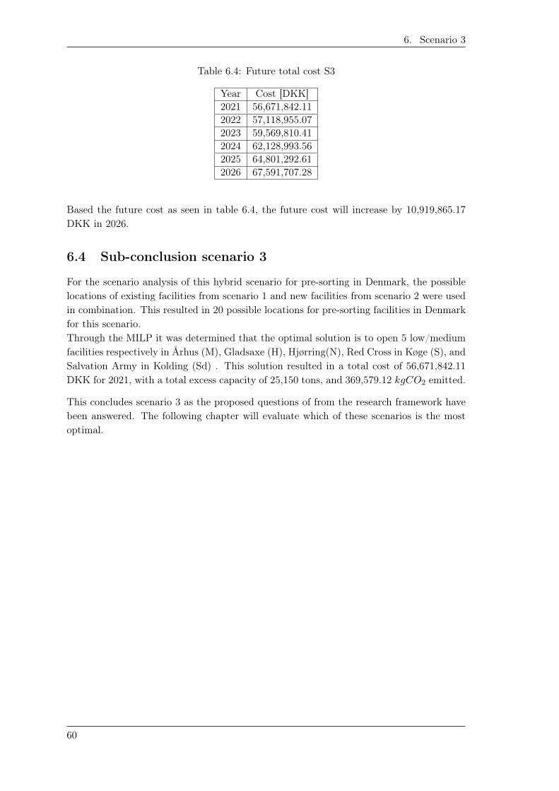
6. Scenario 3


Year Cost [DKK]2021 56,671,842.112022 57,118,955.072023 59,569,810.412024 62,128,993.562025 64,801,292.612026 67,591,707.28

Based the future cost as seen in table 6.4, the future cost will increase by 10,919,865.17DKK in 2026.


For the scenario analysis of this hybrid scenario for pre-sorting in Denmark, the possiblelocations of existing facilities from scenario 1 and new facilities from scenario 2 were usedin combination. This resulted in 20 possible locations for pre-sorting facilities in Denmarkfor this scenario.Through the MILP it was determined that the optimal solution is to open 5 low/mediumfacilities respectively in Århus (M), Gladsaxe (H), Hjørring(N), Red Cross in Køge (S), andSalvation Army in Kolding (Sd) . This solution resulted in a total cost of 56,671,842.11DKK for 2021, with a total excess capacity of 25,150 tons, and 369,579.12 kgCO2 emitted.

This concludes scenario 3 as the proposed questions of from the research framework havebeen answered. The following chapter will evaluate which of these scenarios is the mostoptimal.

60

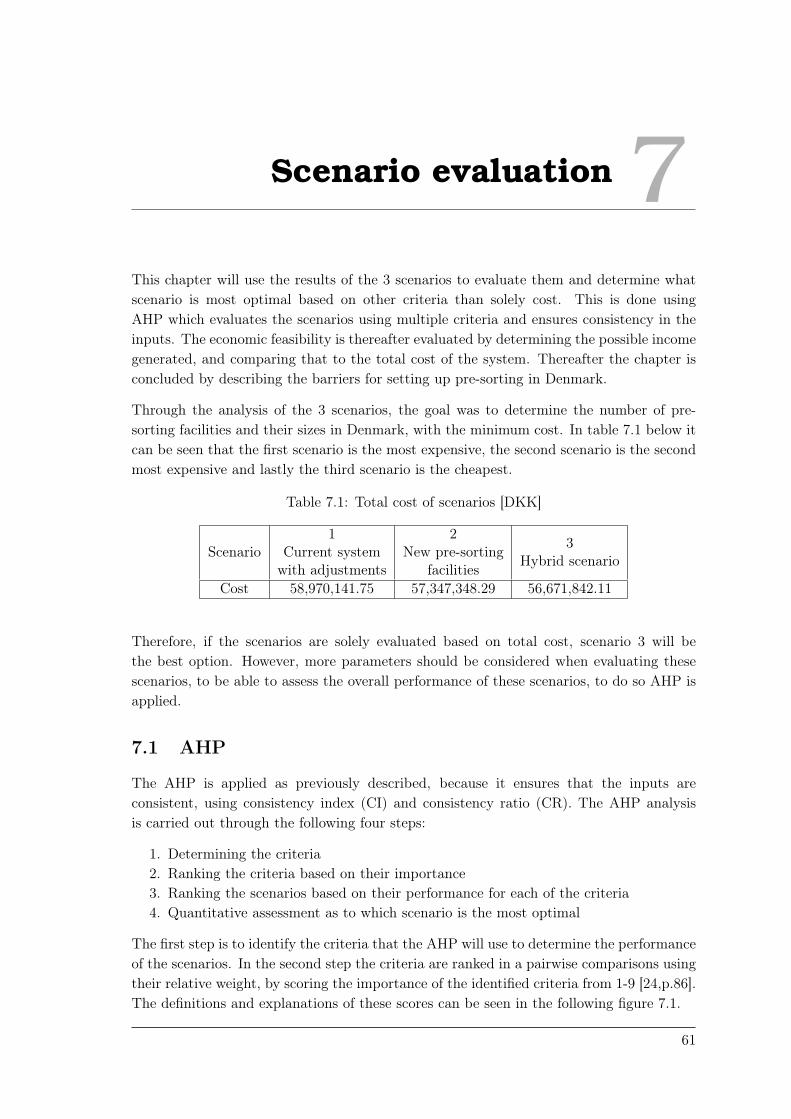
Scenario evaluation 7This chapter will use the results of the 3 scenarios to evaluate them and determine whatscenario is most optimal based on other criteria than solely cost. This is done usingAHP which evaluates the scenarios using multiple criteria and ensures consistency in theinputs. The economic feasibility is thereafter evaluated by determining the possible incomegenerated, and comparing that to the total cost of the system. Thereafter the chapter isconcluded by describing the barriers for setting up pre-sorting in Denmark.

Through the analysis of the 3 scenarios, the goal was to determine the number of pre-sorting facilities and their sizes in Denmark, with the minimum cost. In table 7.1 below itcan be seen that the first scenario is the most expensive, the second scenario is the secondmost expensive and lastly the third scenario is the cheapest.

Table 7.1: Total cost of scenarios [DKK]

Scenario1

Current systemwith adjustments

2New pre-sorting

facilities

3Hybrid scenario

Cost 58,970,141.75 57,347,348.29 56,671,842.11

Therefore, if the scenarios are solely evaluated based on total cost, scenario 3 will bethe best option. However, more parameters should be considered when evaluating thesescenarios, to be able to assess the overall performance of these scenarios, to do so AHP isapplied.

7.1 AHP

The AHP is applied as previously described, because it ensures that the inputs areconsistent, using consistency index (CI) and consistency ratio (CR). The AHP analysisis carried out through the following four steps:

1. Determining the criteria2. Ranking the criteria based on their importance3. Ranking the scenarios based on their performance for each of the criteria4. Quantitative assessment as to which scenario is the most optimal

The first step is to identify the criteria that the AHP will use to determine the performanceof the scenarios. In the second step the criteria are ranked in a pairwise comparisons usingtheir relative weight, by scoring the importance of the identified criteria from 1-9 [24,p.86].The definitions and explanations of these scores can be seen in the following figure 7.1.

61

7. Scenario evaluation

Figure 7.1: AHP scale by Saaty

When comparing criteria A to criteria B, a score of 1 means the two criteria are equallyimportant. Meanwhile a score of 9 means criteria A has extreme importance over criteriaB. A reciprocal score is used when comparing criteria B to criteria A, in this examplethe reciprocal score for criteria B compared to criteria A will be 1/9. The consistencyof these input values are hereafter checked by calculating their CI and CR. The thirdstep is to rank the performance of the scenarios for each criteria using the same pairwisecomparison. The last step combines the criteria weight and ranked performance of thescenarios to determine what scenario is most optimal based on all criteria.

7.1.1 Determining the criteria

The criteria used for this AHP analysis are identified through brainstorming on importantfactors to set up and implement pre-sorting in Denmark, literature research, and aninterview with Nikola Kiørboe. All criteria that have been considered can be seen intable 7.2 below, along with a brief explanation of them.

Criteria Explanation Is it used?

Environmental sustainability

The EU regulation has a focus ondecreasing the negative environmental impact,thereby increase environmental sustainability.

The environmental sustainabilityis measured in CO2 emissions.

Yes

Economic sustainability

A pre-sorting system that is noteconomically sustainable will not be feasible.

If that is the case, then textiles will beincinerated rather than recycled and therebydecreasing the environmental sustainability.The economic sustainability is measured

in the total cost of the scenario.

Yes

62

7.1. AHP AAU

Circularity

A circular pre-sorting system which followsthe waste hierarchy decreases the

negative environmental impact. This ismeasured by the percentage of textiles that

are recycled.

No

Excess capacity

Excess capacity allows the system to copewith increased volumes in the future,

however too high of an excess capacity couldmean resources wasted. Excess capacity

is measured by how many extratons can be pre-sorted.

Yes

Social sustainabilityA social sustainable system

creates jobs for the communityit is placed in.

No

Risk

The risks that are associatedwith setting up a pre-sorting system

should be evaluated to make it possibleto have contingency plans for thesethe risks are measured in severity.

Yes

Table 7.2: Possible criteria for scenario evaluation

Two criteria mentioned in the table are excluded from the AHP analysis, these are Socialsustainability and Circularity. Social sustainability is excluded as the employment ofemployees, living conditions, and medical accessibility do not vary depending on thescenarios, due to the size of Denmark. Circularity is excluded as none of the scenarioswill ensure a fully circular system, but determines the first part of a circular system. Itis still required to decide how the detailed sorting and recycling of used textiles shouldbe done and by whom, to determine if a circular system is a possibility. The remainingcriteria will be used in the AHP, and it will be described in the following how these aremeasured.

CO2 emissions

The amount of CO2 emitted is a critical criteria when evaluating the scenarios, asenvironmental sustainability is a focus point of political parties in both Denmark andin EU, as seen through the EU climate directive on waste [5], and the Danish governmentsclimate plan [7].

Total cost

The cost of setting up and operating the pre-sorting facilities, is a critical criteria toconsider for the scenarios, as too high of a total cost can make it economically unfeasibleto do so. If it is not economically feasible for the companies to pre-sort the textiles, thensome of the textiles will inevitably end up being incinerated rather than recycled. Thisgoes against both the EU directive and the Danish climate plan, and must therefore be

63


prevented. However, the AHP will not determine whether the scenarios are economicallyfeasible, but it will clarify which is the best scenario based on this criteria, and therebythe most likely to be economically feasible.

Excess capacity

Having excess capacity can have both a negative and positive impact on a company. Itcan ensure that a company who is working in a field with rapid growth, has capacity togrow without having to expand their facility. However, having a high excess capacity canalso cause issues because of the investment in resources that could potentially never beutilized. The excess capacity for each scenario will be evaluated by the amount of tons oftextiles that can still be pre-sorted based on the size of the picked facilities.

Risk

For all of the scenarios, the risks connected are important to consider as they can havean impact on the success of the scenarios. The scenarios differ regarding the locationspicked and whether the locations are NGO operated or require a new facility. Due to this,the risks connected and their severity will vary, and therefore it will have an impact onwhat scenario is most optimal. The risks will be measured based on their severity, whichis impacted by the picked locations and operators.

7.1.2 Ranking of criteria

Now that the criteria are determined, the next step is to find the relative weight of thesecriteria in order to rank them based on their importance. This is done in a pairwisecomparison from which the results can be seen in the following figure 7.2 which is fromthe attached appendix B.4 in the sheet ’Criteria’.

Figure 7.2: Criteria scoring

When a criteria is compared to itself it is given a score of 1, meaning it is equally asimportant. When comparing CO2 emissions to the total cost it is given a score of 1/3,meaning that CO2 emissions is slightly less important than the total cost. This score isgiven as the total cost of the scenarios can make them economically unfeasible and therebythe scenario would not be further considered. Therefore, CO2 emissions are weighted lessimportant than the total cost of pre-sorting in Denmark. A reciprocal score is given forthe inverted comparison, meaning when total cost is compared to CO2 emissions it is givena score of 3. The reciprocal scores are not further explained for the remaining criteria,as the same method is used. Comparing CO2 emissions to excess capacity a score of 3is given, meaning that CO2 emissions is slightly more important than excess capacity, as

64

7.1. AHP AAU

having excess capacity will not necessarily make the scenario unfeasible, but having veryhigh CO2 emissions will be more likely to make it unfeasible. Comparing CO2 emissionsto risk is given a score of 5, meaning CO2 emissions has a higher impact on which of thescenarios is the best option. This score is given as risks may not have any impact if thereare no risks of a higher severity.When comparing total cost to excess capacity a score of 5 is given, meaning total cost has aslightly higher impact, as excess capacity will not necessarily make the scenario unfeasible,while total cost may. When comparing total cost to risk a score of 7 is given, meaningtotal cost is more important than risk, as risks might not have any impact on the scenarios.When comparing excess capacity to risk a score of 3 is given, meaning excess capacity hasa slightly higher impact than risk.After having scored all criteria, next these scores are used to determine the relative weightof the criteria. To do so the sums of these scores are firstly calculated, which can be seenin figure 7.2 above, in the bottom row. This sum is used to calculate an input to thestandardized matrix, this is done by the given score of a comparison being divided by thesum of the column. For CO2 emissions compared to CO2 emissions the calculation wouldbe Pairwise comparison value

Sum of column = 14.53 = 0.22. This is done for all scores in the matrix, and the

results can be seen in the following figure 7.3.

Figure 7.3: Standardized matrix criteria

The weight of each criteria is then calculated based on these inputs, this is done by dividingthe sum of the row by the number of evaluated criteria. For the CO2 emissions row, thecalculations can be seen in equation 7.1. This is done for all rows, and the results canbe seen in figure 7.3 in the column ’Weight’. Based on these inputs the most importantcriteria is the total cost (55.8%), followed by CO2 emissions (26.3%), then excess capacity(12.2%), and lastly risk (5.7%).

Weight (criteria) =Row values

Number of criteria

Weight (CO2 emissions) =0.22 + 0.20 + 0.32 + 0.31

4∗ 100% = 26.3% (7.1)

To determine if these inputs are consistent, the CR should be calculated. The inputs areconsistent if 0 ≤ CR < 0.1, meaning the CR must be more than or equal to 0 and less than0.1. Before the CR can be calculated, the CI must be determined. To determine the CI thefollowing formula is firstly applied to calculate the weighted sum {Ws} = [C]{W}, where[C] is the pairwise comparisons from figure 7.2, and {W} is the weight of the criteria fromfigure 7.3. For CO2 emissions compared to itself the calculation would be the following:{Ws} = [C]{W} = 1 ∗ 26.3% = 0.26. This is done for all combinations of the matrixand the results can be seen in the following figure 7.4.

65


Figure 7.4: Ws input to the CI & CR calculations

Hereafter, the row sum Sum(W_s) for each criteria is calculated, the results can be seenin figure 7.4 in the ’Sum(W_s)’ column. This is used to calculate the consistency vectorusing the following formula: Consistency vector = {Sum(W_s)

W }, and the results of thiscalculation is seen in figure 7.4 in the ’Consistency vector’ column. This is now used tocalculate the average value of the consistency vectors, the calculation of this can be seenin equation 7.2 below.

Average value of consistency vectors =4.17 + 4.22 + 4.04 + 4.04

4= 4.118 (7.2)

Now these values can be used to calculate the CI which uses the following formula 7.3,where n is the number of criteria [40,p.965].

CI =Average value of consistency vectors − n

n− 1=

4.118− 4

4− 1= 0.039 (7.3)

With the CI calculated to be 0.039, the next step is to calculate the CR, which is done inthe following equation 7.4. In this formula, the ’Random Consistency Index’ depends onthe number of criteria that are evaluated, and it is given by Thomas L. Saaty who inventedthe AHP method. Seeing as there are 4 criteria used in the AHP, the random index is0.90.

CR =CI

Random Consistency Index=

0.039

0.90= 0.044 (7.4)

With the CR calculated to be 0.044 the input values are considered consistent, as the CRfulfills its constraints: 0 ≤ CR < 0.1. This concludes the second step of the AHP ofranking of the criteria by their importance.

7.1.3 Ranking of scenarios

The third step of the AHP is to rank the scenarios for each criteria, using the same methodas in the previous step. Seeing as the AHP method was described in detail in the previousstep, these subsections will only present the scores and CR values. The full calculationscan be seen in the attached appendix B.4.

66

7.1. AHP AAU

CO2 emissions

Through the scenarios the amount of CO2 emitted was determined. The results of thiscan be seen summarized in the following table 7.3, which shows the total distance in kmand the kgCO2 emitted per scenario.

Table 7.3: Distance [km] and kgCO2 emitted per scenario

Scenario Distance [km] kgCO2e

1 351,038 507,2692 261,989 378,5893 255,754 369,579

As seen in table 7.3 scenario 3 emits the least CO2, and therefore performs best regardingthis criteria. These results are now used to score the scenarios and calculate the CR, thefull calculations for this can be seen in the attached appendix B.4 in sheet ’CO2 Emissions’.When scenario 1 is compared to scenario 2 it is given a score of 1/4, meaning scenario 1performs worse than scenario 2. This score is given seeing as scenario 1 emits the most CO2

and roughly 127,000 kg more than scenario 2. When scenario 1 is compared to scenario 3it is given a score of 1/5, meaning scenario 1 performs much worse than scenario 3. Whenscenario 2 is compared to scenario 3 it is given a score of 1/2, meaning scenario 2 performsslightly worse than scenario 3. This score is given as scenario 3 emits roughly 9,000 kgCO2

less.

Figure 7.5: Scores per scenario for CO2 emissions

With the scores given as seen in figure 7.5, the same method is applied as with the criteriato calculate the CR. The results of this results in a CR of 0.021 meaning the inputs arevalidated as being consistent. This concludes the CO2 emissions comparison, and thefollowing subsection will evaluate the total cost of the scenarios.

Total cost

Through the scenarios the total cost of setting up a pre-sorting system was determined,these costs can be seen below in table 7.4.

Table 7.4: Total cost per scenario [DKK]

Scenario Total cost1 58,970,141.752 57,347,348.293 56,671,842.11

67


Based on the results seen in table 7.4, scores are given for each scenario. When scenario 1is compared to scenario 2 it is given a score of 1/3, meaning scenario 1 performs slightlyworse than scenario 2 in terms of total cost. This score is given seeing as there is differenceof roughly 1,600,000 DKK between the two scenarios. When scenario 1 is compared toscenario 3 a score of 1/5 is given, meaning scenario 1 performs much worse than scenario3. When comparing scenario scenario 2 with scenario 3 a score of 1/2 is given, meaningscenario 2 performs slightly worse than scenario 3, due to the roughly 700,000 DKK dif-ference between the two scenarios. The following figure 7.6 contains all the scores, and thecalculations can be seen in the attached appendix B.4 in the sheet ’Total cost’.

Figure 7.6: Scores per scenario for total cost

Using these scores a CR of 0,016 is found, the inputs are therefore validated as beingconsistent, and this concludes the cost comparison. The following subsection will evaluatethe excess capacity of the scenarios.

Excess capacity

Through the MILP the excess capacity was determined for each of the scenarios, a summaryof these results can be seen below in table 7.5.

Table 7.5: Excess capacity per scenario [tons]

Scenario Excess capacity1 32,0112 22,1023 25,150

As seen in table 7.4 scenario 1 has the highest amount of excess capacity. The closer ascenario is to the required excess amount of 13,249 tons, the better it will perform. This isbecause having a lot of unnecessary excess capacity will tie up monetary resources, basedon these excess capacities the following scores are given. When scenario 1 is compared toscenario 2 a score of 1/5 is given, meaning scenario 1 performs much worse than scenario 2.This score is given seeing as scenario 1 has roughly 10,000 tons more excess capacity thanscenario 2. When scenario 1 is compared to scenario 3 a score of 1/3 is given, meaningscenario 1 performs slightly worse than scenario 3. This score is given seeing as scenario1 has roughly 7,000 tons more excess capacity. When scenario 2 is compared to scenario3 a score of 3 is given, meaning scenario 2 performs slightly better than scenario 3. Thisscore is given seeing as scenario 2 has roughly 3,000 tons less excess capacity. A full list ofthese scores and the reciprocal scores can be seen in figure 7.8, and the calculations canbe seen in attached appendix B.4 in sheet ’Excess capacity’.

68

7.1. AHP AAU

Figure 7.7: Scores per scenario for excess capacity

The CR for these inputs equals 0.033, thereby validating the consistency of these. Thisconcludes the excess capacity comparison, the following subsection will compare the riskof the scenarios.

Risk

To determine if the risk varies between the scenarios, all the risks and the severityassociated with them must be identified. Through brainstorming and literature researchthe following risks were identified.

• Incorrect citizen use• Low per-capita disposal• Low future demand for recyclables• Political focus• Investment risk• Negative growth of recyclables in the market

The first identified risk is incorrect citizen use of the used textile system, this risk occurswhen citizens deliver used textiles to the wrong actor, e.g. WMCs receiving reusabletextiles. The next risk is low per-capita disposal of used textiles through the separatecollection system. This occurs when citizens keep textiles in their home rather thandisposing of them or dispose of them through systems that are not intended for usedtextiles such as household waste. Low future demand of recyclables impacts the pre-sortersby having fewer potential buyers, and thereby decreasing the potential income made fromselling these recyclable textiles. These risks do not vary depending on the scenarios, andthey are therefore not included in the scoring of the scenarios.Three risks were identified where the severity is higher for new facilities then for NGOswith existing facilities, these are risk of shift in political focus, risk of investment, negativegrowth of recyclables in the market, and low future demand for recyclables. If the politicalfocus shifts and for example the requirement of the pre-sorter to be a private companyis removed, there is a chance the WMCs will perform the pre-sorting themselves. If thatis the case, then all pre-sorting facilities will receive less recyclables and textile waste,resulting in higher excess capacity for pre-sorting. The NGOs could use this capacity forsorting reusable textiles instead, whereas new facilities would have to set up entirely newprocesses. The investment required is also lower for a NGO as they will only expand theirfacilities instead of setting up entirely new ones, making the investment risk higher fornew facilities. If the future volume of recyclables and textile waste is decreasing, then theallocated capacity for a NGO facility can still be used to sort reusable textiles, while newfacilities would have higher excess capacities. For these reasons, scenarios that use newfacilities rather than existing facilities from NGOs will have higher risks associated.

69


Based on this information the following scores are given. When comparing scenario 1 toscenario 2 a score of 4 is given, as scenario 2 only uses new facilities while scenario 1 onlyexpands established facilities, therefore the risks associated are lower for scenario 1. Whencomparing scenario 1 with scenario 3 a score of 3 is given, as some of the facilities inscenario 3 are new and some are expansions. When comparing scenario 2 to scenario 3 ascore of 1/3 is given, meaning scenario 2 performs slightly worse than scenario 3 based onrisks. This score is given as scenario 2 only uses new facilities, and scenario 3 uses someof both. Below in figure 7.8 a full list of the input values can be seen, and the calculationscan be seen in the attached appendix B.4 in sheet ’Risk’.

Figure 7.8: Scores per scenario for risk

Based on the input scores, the CR is calculated being 0.064 which thereby validates theconsistency of the inputs. This concludes the second step of the AHP, and the next stepwill assess the overall performance of the scenarios.

7.1.4 Assessment

The following figure 7.9 summarizes the scores given for each of the scenarios and theweight of the criteria. This information is used to determine the overall sum of theseinputs, this indicates which scenario is the most optimal based on the criteria. This iscalculated by multiplying the individual score of the scenario in each criteria with theweight of the criteria from figure 7.3. An example of this calculation for scenario 1 wouldbe the following; 0.10 ∗ 26.3%+0.12 ∗ 55.8%+0.11 ∗ 12.2%+0.61 ∗ 5.7% = 14.18%. Thisis done for all scenarios, and the results can be seen in the ’Sum’ column of figure 7.9.

Figure 7.9: AHP results

From this it can be concluded that scenario 3 is most optimal based on the criteria, with ascore of 51.08% of a total 100% given. Scenario 3 performs best in the two most importantcriteria CO2 emissions and total cost, in the other two criteria excess capacity and riskit performs second best. This concludes the AHP assessment, and the following sectionwill now evaluate the economic feasibility of the optimal scenario as found by through theAHP.

70

7.2. Economic feasibility AAU

7.2 Economic feasibility

The AHP analysis concluded that scenario 3 was the best scenario of the 3 based on thechosen criteria, however whether it is economically feasible is yet to be determined. Toestablish this, it must be identified if there are any additional costs occurring after the pre-sorting has been done and if there is any income from the recyclable textiles. The scenariois economically feasible when the generated income outweighs the total cost, meaning thereis a profit instead of a loss.

In section 3.3 in the preliminary chapter it was determined that in 2016, 10,218.40 tons oftextile waste are part of the volume that must be pre-sorted. When applying the yearlygrowth of 4.42 % for 5 years, the amount of textile waste in 2021 is 12,685.32 tons. Afterbeing sorted out during the pre-sorting process, this volume of textile waste has to besent to be incinerated or landfilled which will result in additional cost. It was informedby Steen Trasborg, that this costs approximately 60 e/ton of textile waste, which equalsto 446.19 DKK/ton. When applying this cost to the volume of textile waste from 2021,an additional 5,660,063 DKK have to be added to the total cost. This means that thepre-sorting of all received textiles and the handling of textile waste results in a total lossof 62,331,905.11 DKK as opposed to the previous loss of 56,671,842.11 DKK.

In addition to the textile waste, also the assumed 11% of reusable textiles are sorted outduring the pre-sorting process and have to be handled afterwards. In 2021, the amountof reusables corresponds to 5,438.35 tons, which are in accordance with the new law,presumably given to NGOs. Therefore, no additional income nor cost is assumed for thereusable textiles.

In the preliminary chapter in section 3.1 it was specified that the recyclable textiles will besent to SIPTex in Malmø. It is informed from actors that it costs approximately 60 e/tonof recyclable textile to be sorted at SIPTex, which equals to 446.19 DKK/ton. In order todetermine the total cost associated with getting the recyclable textiles sorted at SIPTex,only the actual volume of recyclables will be considered. In 2016, the volume of recyclableswas 29,606.60 tons as determined in section 3.3 in the preliminary analysis chapter, andwhen applying the yearly growth of 4.42% for 5 years, the volume of recyclables for 2021is 36,754.2 tons. When these 36,754.2 tons are sorted at SIPTex for 446.19 DKK/ton,it results in an additional cost of 16,399,356.5 DKK. When this is added to the cost ofpre-sorting of 62,331,905.11 DKK in 2021 which includes handling waste, it results in atotal loss of 78,731,261.61 DKK as there is assumed to be no income generated.Having the recyclables sorted at SIPTex is what should be done to keep transportationat a minimum, as it is the only automated sorting facility in the Nordics with availablecapacity to receive recyclables. However, because there is currently no income when pre-sorting recyclables and textile waste, the recyclables could be sold to other countries wherethey could generate a small income, depending on whom they are sold to.

It is known that the price for recyclable textiles has rapidly decreased over the past years,as it can be seen in figure 7.10 below. This graph shows the price development over thepast 4 years, when ARWOS sells one ton of recyclables, as informed by Kresten Thomsen.

71


Figure 7.10: Price development

In the figure it can be seen, that the price for 1 ton of recyclables is rapidly decreasingand reached 0 DKK/ton in 2021. The orange columns show the price per ton per year,and the dotted blue line is a trend-line which indicates how ARWOS assumes the futuredevelopment of prices for recyclables to be. If it is assumed that this is the price there ispayed for recyclables it will give a total loss of 62,331,905.11 DKK.

Steen Trasborg informed that their current income from selling recyclable textiles tocustomers in Eastern Europe is 0.003 DKK/kg, and similar to ARWOS they are seeinga rapidly declining price development. If the income of 0.003 DKK/kg or 3 DKK/tonis applied to the current volume of recyclables, an income of 110,262.60 DKK will begenerated when pre-sorting and selling 36,754.2 tons in 2021. Out of the total cost of62,331,905.11 DKK for scenario 3 including the cost for handling textile waste, the incomeof recyclables will cover 0.18% and thereby result in a total loss of 62,221,642.51 DKK.

After having investigated all the possibilities of what can happen to the recyclable textilesafter the pre-sorting of them has been done, it can be concluded that all of the optionswill end out in an economically unfeasible solution. This is because all options currentlyavailable for disposing of the pre-sorted recyclables will generate a total loss for thecompany. This loss is assumed to be the responsibility of the municipality as they arethe ones paying for having the recyclables and textiles waste pre-sorted.

7.3 Barriers and benefits for pre-sorting in Denmark

The largest barrier for setting up pre-sorting facilities in Denmark is the economicfeasibility because the income of selling recyclable textiles does not cover the cost ofpre-sorting and handling the pre-sorted textiles. The results depending on where therecyclables are sent after pre-sorting can be seen in table 7.6 below.

Table 7.6: Summary of economics

Option -446.19 DKK/tonSIPTex

0 DKK/tonARWOS customer

3 DKK/tonTrasborg customer

Total loss 78,731,261.61 DKK 62,331,905.11 DKK 62,221,642.51 DKK

72

7.3. Barriers and benefits for pre-sorting in Denmark AAU

Knowing how large of a loss there is associated with operating pre-sorting facilities, it canbe investigated how much income there hypothetically is required to break-even. This willbe done using two different approaches, one where the government is assumed to coverthe loss of the facilities by compensating per ton of textile pre-sorted. Because it is inthe interest of the Danish government to ensure that textiles are reused and recycled,it can be assumed that they might have incentive to support the companies who set uppre-sorting facilities through financial aid. The other approach is assuming that SIPTexwould pay the pre-sorting facilities per received ton of recyclables. In the current market,this approach does not have a high likelihood of occurring. However if the demand ofrecyclables does increase so will the number of sorting facilities, and thereby the price ofsorting will decrease or even turn into a profit.

Firstly, the required income from the government per ton of pre-sorted textile in 2021to break-even, is determined in the following equation 7.5, following the assumption thatrecyclables are sorted at SIPTex for the current cost of 446.19 DKK/ton. This calculationis done also assuming that if the facilities receive money from the government they will bepayed per ton pre-sorted and not receive a fixed income.

Required income from government =Total cost

V olume of pre− sorted textiles

=78, 731, 261.61 DKK

54, 878 tons= 1, 434.66 DKK/ton (7.5)

Secondly it can be determined what the income per ton of recyclables from SIPTex shouldbe in order to cover the total cost of pre-sorting and break-even. For 2021, the calculationcan be seen in equation 7.6 and it results in a required income of 1,695.91 DKK per tonof recyclables.

Required income from SIPTex =Total cost

V olume of recyclables

=62, 331, 905.11 DKK

36, 754.20 tons= 1, 695.87 DKK/ton (7.6)

Another barrier that was identified through interviews with actors and experts in the usedtextile industry, is that the politicians have put the responsibility of taking the next stepsfor setting up this system onto the actors. However, these actors are not willing to take thisresponsibility, as there is currently no possibility to generate an income, which makes iteconomically unfeasible for them to take part in the pre-sorting. Therefore, the actors arewaiting for further law changes to be made or development of a monetary compensationsystem, which would aid the economic feasibility. The separate collection system will beimplemented from January 1st 2022, and currently there are no actors to perform thepre-sorting, sorting and recycling of the used textiles after the collection. This meansthat there are uncertainties in the future for all involved actors in the industry, resultingin them not wanting to make major changes and investments. This is further impacted

73


by the lack of R&D in the used textile industry, therefore making it hard to make wellinformed decisions. This lack of R&D also limits the innovation in the pre-sorting process,thereby forcing the pre-sorting to be carried out in manual processes which are costly.Automated processes could decrease the cost per tons of pre-sorted textile, and therebyincrease the likelihood of a economic feasible pre-sorting system in Denmark.

There are potential benefits of pre-sorting recyclables within Denmark for the purpose offurther recycling the textiles. The main possible benefit is the CO2 savings that recyclingcan bring, this is because the recycled textiles will be used for production of productsthat has the potential to replace the production of new ones. This will thereby reducethe amount of CO2 emitted from producing new textiles, and no virgin materials will beused for this process which delimits the depletion of natural resources. The exact CO2

saving will vary depending on two parameters; the fiber composition of the textile andthe recycling process applied. Currently there is no accurate data on the general fibercompositions of Danish used textiles, which thereby makes it impossible to accuratelydetermine the CO2 savings. The exact recycling process applied is also unknown, ascurrently no established facilities are doing this process in Denmark. It is assumed thatthere will be a CO2 benefit of pre-sorting, it is however not possible to determine thisexact scale.

7.4 Sub-conclusion scenario evaluation

For the evaluation of the analysed scenario, AHP was applied. As the first step of theAHP, the following 4 criteria were determined to be suitable for the evaluation of thescenarios; environmental sustainability, economic sustainability, excess capacity, and risk.Of these the environmental sustainability is measured in CO2 emissions, and economicsustainability in total cost.When ranking these criteria in terms of their relative importance, it was found that totalcost is most important with a weight of 55.8%, followed by CO2 emissions with 26.3% andexcess capacity with 12.2%, and risk is least important with a weight of 5.7%.After scoring the scenarios for each criteria, the AHP assessment showed that scenario 3scores best overall regarding the 4 criteria, followed by scenario 2, and scenario 1 scoredworst.Through the comparison of the total cost and possible income for scenario 3 it was foundthat it is not economically feasible to set up pre-sorting facilities in Denmark, as the costis much higher than any potential income.The economic feasibility was determined to be the largest barrier for pre-sorting inDenmark. It was found that an income of 1,434.66 DKK per ton of pre-sorted textileis required from the government in order to cover the total costs, or an income of 1,695.87DKK per ton of recyclables from SIPTex. Another barrier was seen in neither politiciansnor actors wanting to take on responsibility for changes in the system. Also the lackof R&D in the field of used textiles was found to impact the economic feasibility, andtherefore as another barrier. As a possible benefit from pre-sorting in Denmark it wasfound that there might be CO2 savings from recycling compared to new production oftextiles, however it was not possible to quantify the impact of this.

74

Discussion 8The purpose of this chapter is to discuss the results found throughout the report, and it isdivided into the 3 parts; preliminary analysis, scenario analysis, and scenario evaluation.

8.1 Preliminary analysis

Required pre-sorting levelIn the preliminary chapter it was assumed that all recyclables from the pre-sorting willbe sent to SIPTex for further sorting. This assumption was made because it was the onlyautomated sorting facility in the Nordics who at the time had capacity available to receivevolumes. However, SIPTex currently has a capacity of 24.000 tons per year, meaning thatthey can not receive the full Danish volume of 36,754.2 tons in 2021 for further sorting, asit has been assumed throughout the report. Through research it was not possible to findany automated sorting facility that is capable of receiving the full Danish volume. If therecyclables were to go to another automated sorting facility, it could change the level thatthe textiles should be pre-sorted to and thereby the employee productivity, which coulddecrease the feasibility of the pre-sorting system. Sending the recyclables to a differentautomated sorting facility can also mean a different price per ton sorted and thereby endup in a different total cost.

Current actorsFor the scenario analysis, the 6 main actors in the current used textile industry in Denmarkwere included as found in literature, which are responsible for the separate collection andhandling of approximately 60% of the Danish used textiles. Additional actors could havebeen included in the analysis, seeing as actors who make up 40% of the current separatecollection are not included such as Blue Cross and Folkekirkens Nødhjælp (DanChurchAid).Adding these actors would increase the number of potential pre-sorting facilities, whichcould lead to a different optimal solution.

Current and future volumesWhen determining the volume of used textiles for pre-sorting in the preliminary analysis,the fractions of recyclables and textile waste from different waste streams were addedtogether as found in data from 2016. From this, overall quality ratios are applied forthe streams of separate collection, being 19% recyclables and 11% textile waste, andmixed collection, being 63% recyclables and 14% textile waste. Instead of applying theseoverall ratios to find the volumes of recyclables and textile waste, these quantities couldbe researched in more detail by investigating the individual actors of each stream. For thevolumes in separate collection, all collection actors e.g. Red Cross and Trasborg, could becontacted and questioned on the amount of recyclables and textile waste in their collected

75

8. Discussion

used textiles. For the mixed collected, which consists of bulky waste, small combustibles,and household waste, the ratios of recyclables and textile waste in the 3 streams could beinvestigated separately. For this report, this detailed approach could not be applied, assome actors do not collect this required data, and it is not available for some waste streamse.g. bulky waste. If the data was available, a more accurate volume of recyclables andtextile waste could have been found, which could have lead to a change in the requiredcapacity, and therefore a different total cost.

Furthermore, an additional 11% were added to these volumes of recyclables and textilewaste, in order to account for reusable textiles that are disposed of wrongfully. These11% was based on information received from by an actor in the industry based on theirobservations. This number could be validated by collecting observations from other actorsif available, or conducting test studies. If a different fraction of reusables were to be found,the required capacity of pre-sorting facilities could change due to changing volumes, andtherefore affect the total cost of the scenarios.

In order to determined the expected future volume for pre-sorting in Denmark, a yearlychange of used textile collection had to be determine in the preliminary analysis. Asthere was no valid data available for Denmark, numbers from a comparable countrywith available and consistent data had to be found. For this, the USA was found beingeconomically similar to Denmark and therefore the yearly growth for the US was calculatedand applied to the Danish used textile volume. The results for expected future volumescould be more accurate if there was data available about the yearly changes in Denmark,or if a more fitting country in comparison had data available. For the calculation of theexpected future volume in Denmark it was then assumed that the found yearly growth of4.42% continues to occur yearly in the future, leading to a linear increase of used textilesover the next years. This assumption was made due to missing information about changesin the increase, however there are growing numbers of measures taken nationally andinternationally to decrease the textile consumption. This means that the applied yearlyincrease of 4.42% could be set to high for the future years, meaning that the calculatedfuture volumes could be too high. If a more accurate, possibly lower yearly change wasapplied, the future volume might be lower and therefore the required excess capacitywould also be lower. This would thereby lead to lower capacity options being chosen forthe scenarios and less employees required, leading to a lower total cost.

Capacity options for pre-sorting facilitiesA set number of capacity options were used for the MILP to choose from to ensure that theinputs to the MILP did not exceed the input limitations from the Excel solver software.A more optimal solution might be possible to find if more capacity options were included,or no limitations were set at all, seeing as the total excess capacity could be closer to therequired and thereby the total cost could decrease. This was however not possible due tothe software limitations, and the 5 capacity options were therefore applied for the scenarios.The set capacities were determined based on the 2021 volume of used textiles, however ifinstead the required 2026 volume was used, different facility sizes might have been chosenthroughout the MILP. This could have impacted the final result of the scenarios throughthe total cost and excess capacity, however it is uncertain whether the impact would havebeen beneficial or disadvantageous.

76

8.1. Preliminary analysis AAU

In the preliminary analysis it was assumed that the pre-sorting facilities would operatewith one shift a day. This assumption impacted the size of the facilities and thereby thefixed cost. If multiple shifts were used instead it could have lead to smaller facilities beingrequired, and thereby decrease the fixed and total cost.

Variable costWhen calculating the environmental cost, a carbon equivalent conversion factor had to beused as input to the formula. To determine this carbon equivalent conversion factor, theweight of the truck and load had to be assumed, and an average weight of 17 tons or greaterwas used. However, it was not specified in the used source if the applied weight is only loadweight or gross weight including the truck weight. For this report, the gross weight wasused in order to account for the worst case scenario, as the higher weight lead to a highercarbon equivalent conversion factor and therefore higher environmental cost. If instead thecarbon equivalent conversion factor of the truck load weight was used, the environmentalcost would have decreased. However, it would not have lead to a great difference in thetotal cost as the environmental cost is only a small fraction of the total cost. However, theenvironmental impact would vary as the CO2 emissions will differ depending on this.

When finding employee wages, there are three types of employees considered in theanalyses; pre-sorters, production manager and drivers. However, when running a pre-sorting facility there are more employees required that were not considered, like cleaningand administrative staff. If these employees were taken into account the cost of runningthe pre-sorting facilities would increase.

When calculating the pre-sorter wage as part of the variable costs, an employeeproductivity of 1,200 kg per workday was used. These numbers were used becauseit was the information there was provided by Steen Trasborg, who is an actor in theindustry. However, the results for pre-sorter wages could be more accurate if the employeeproductivity would instead have been measured in a test study using the determined pre-sorting level required. A different employee productivity could have lead to a differentpre-sorter wage per ton of pre-sorted textile, and thereby change the total cost of thescenarios.

The employee wages for pre-sorters and production managers were determined usingaverage wages from the positions in the industry that were assumed to fit the requirementfor the employees in the pre-sorting system. For the pre-sorters it was the hourly wage of anunskilled employee, and for the production managers it was the monthly wage of a generalproduction manager. However, the requirements for these employees could be different,in regards to e.g skill level, which could result in different average wages and therefore indifferent total costs for the scenarios. More accurate inputs for the hourly wages could befound by conducting test studies, or by further research on existing positions in the usedtextile industry.

The driver wages were calculated using the weighted kilometers multiplied by the averagepay per km driven. This calculation was used because it could not be determined how manydrivers were needed to transport the used textile volumes as it is assumed that all WMCshave their own drivers hired, also defining how long the required trips would take wasnot possible. If it was possible to find these inputs to determine the driver wage through

77

8. Discussion

average salary and distances driven, the drivers salary could vary, however whether thisdifference would be beneficial or disadvantageous in terms of cost cannot be determined.

Fixed costIt is assumed that the facilities will be rented by the company, however in real life thefacilities will most likely be bought by the companies operating them. This would lead toa much higher opening cost, and the monthly payment would most likely be the paymenton the loan. If this is the case, then after a certain amount of years there will no longerbe a monthly payment on a loan, which could result in a different total cost.

In the preliminary chapter it was assumed that expanding a facility would cost 200,000DKK, and opening a new facility would cost 500,000 DKK. It would have been moreaccurate to find examples of these costs, however as no comparable costs were found theyhad to be assumed. If examples were found the cost of these may have increased, whichcould impact the MILP choices of facilities by choosing to open or expand fewer facilities.In contrast, if examples were found where the cost was lower, then the MILP could havechosen to open or expand more facilities.

8.2 Scenario analysis

In scenario 2 and 3 the 3 biggest cities København, Frederiksberg and Gentofte of theHovedstaden region were not included as no suitable production facilities were found. Thethree following largest cities were therefore chosen which impacted the MILP by increasingthe cost of transportation. However, if a renting price was assumed for these cities theycould be included in the MILP analysis. This could lead to different facilities being chosen,which could decrease the transportation cost. It is however uncertain if this would outweighthe renting cost, so the total impact can not be determined.

Weighted km was used as the average distance from each region to each possible facility inthe MILP analysis. This distance had to be used as the WMCs were divided into regionsto limit the number of variables in the MILP. If the individual WMCs were included in theMILP it could have resulted in a different optimal solution, which could have decreasedthe total cost and thereby the economic feasibility of the solution. To do this, softwarethat has a higher limit for the number of variables it allows would have to be used.

In the MILP, one of the constraints was that the excess capacity of the total system hasto be larger or equal to the required volume in 2026. As the excess capacity is set for theentire system and not the individual facilities, the excess capacity will not necessarily beevenly distributed between the facilities. This could mean that the facilities who have ahigh excess capacity are the ones who are located in regions with a low population andthereby low volume of recyclables and textile waste. Which will mean the higher populatedarea facilities will quicker reach the capacity limit and then the textiles have to be sent to adifferent facility resulting in higher future cost impacted by the transportation. To ensurethat the excess capacity will be evenly distributed according to the volume of the regions,there can be set a capacity requirement per region. However doing this will require theMILP to set up a minimum of one facility in every region. This could contradict the goalof minimizing the total cost, due to higher employee wages in some regions and thereforemight not necessarily yield in the most optimal result in terms of cost.

78

8.3. Scenario evaluation AAU

8.3 Scenario evaluation

When evaluating the scenarios and the chosen criteria, the AHP method was used. Thescores for the AHP were determined through interviews with experts in the field and carefulconsideration, however the validity of inputs could be increased further in order to get amore accurate result. To increase the validity the subjectivity of the scores would haveto be decreased, to do so more experts would have to be consulted to validate the givenscores. By consulting additional experts more criteria could be identified, which couldresult in a different optimal scenario.

Throughout the report the facilities were chosen to decrease the total cost throughminimizing cost of transportation and pre-sorting, however in real life the closest facilitymay not necessarily be the one which offers the lowest bid. In real life the lowest bidwill always be chosen, unless there are other incentives to effect this decision, e.g. CO2

emission of the transportation. It is however not possible to further analyse this in thisproject, and therefore the choice of pre-sorting facilities are based on the fixed and variablecosts, because these costs are assumed to be used as an input to determine the bids.

It was assumed that the reusable textiles would be given to the NGO, as according to theDanish regulations NGO should receive reusable textiles. It is however uncertain whatNGO the textiles should go to and how this would be determined. The choice of whatNGO it is sent to could also impact the economic feasibility of the pre-sorting facilitydepending on who pays for the transportation, packing, and whether the NGOs shouldpay for the reusable textiles.

The number of employees required for each facility is determined based on the yearlyvolume of textiles that each facility must pre-sort. It is however uncertain if this numberof employees will vary throughout the year, based on seasonal variation in the generationof used textiles. If there is a variation in the volume of textiles throughout the year, thenthe number of workers required will also vary throughout the year. To determine this afurther analysis is required which evaluates the seasonal variation. This is however notpossible within the scope of this report, and an uniform distribution of the textile volumethroughout the year is therefore assumed.

79

Conclusion 9The goal of this project was to evaluate if setting up a pre-sorting system in Denmarkis economically feasible and how large its environmental impact will be. To answer this,literature was reviewed to identify analytical methods that should be applied. A researchframework was developed, which described the theoretical plan of how the identifiedmethods would be adapted and applied, to the three scenario that were developed.Throughout the preliminary analysis, it was determined that the required pre-sorting levelof the system will be the same as the requirements of SIPTex, meaning that the textileshave to be manually pre-sorted into recyclables, reusables and textile waste. This wasdetermined as SIPTex was the only automated sorting facility in the Nordics who canreceive volumes from other countries. Hereafter 6 current main actors were identified as,Trasborg, Red Cross, Salvation Army, UFF, Danmission and DanChurch Social. None ofthese actors were deemed capable of pre-sorting the recyclables and textile waste, withoutany adjustments being made to their business. Using historical data from 2016, the currentvolume of recyclables and textile waste was determined by applying a yearly increase of4.42% to be 54,878 tons in 2021 and the expected volume in 2026 was also calculated.Hereafter the most suitable transportation mode was determined to be a 40 ft tippingcontainer truck on road which can contain a load of 10.14 tons.The costs for pre-sorting was divided into variable- and fixed-costs, which consist ofdifferent sub parts. Variable cost consisted of transportation cost, which is further dividedinto environmental- and fuel-cost, and employee wages, which are further divided into pre-sorter-, production manager-, and driver-wages. The fixed cost was found to consist of therenting-, opening-, and expansion-cost. The environmental impact of the scenarios weredetermined to be measured through CO2 emissions.

The first scenario investigated the possibilities of pre-sorting in Denmark using the currentsystem with adjustments. Throughout this scenario analysis it was found that 3 of thecurrent main actors were interested in making adjustments and perform pre-sorting inDenmark, these being Red Cross, Salvation Army and Trasborg. Through the MILP itwas determined that for this scenario, the optimal solution is to open 3 medium facilitiesrespectively at the locations of Red Cross in Horsens (M), Trasborg in Taastrup (H), andSalvation Army in Kolding (Sd). This solution resulted in a total cost of 58,970,141.75DKK for 2021, with a total excess capacity of 32,011 tons, and 507,269.2 kgCO2 emitted.The second scenario looked into setting up new facilities for pre-sorting in Denmark, thepossible locations were determined based on population centers. Through this scenarioanalysis it was determined that the optimal solution is to open 3 low/medium facilitiesrespectively in Aalborg (N), Viborg (M) and Odense (Sd) and one medium facility inGladsaxe (H). This solution resulted in a total cost of 57,347,348.29 DKK for 2021, with

80

AAU

a total excess capacity of 22,103 tons, and 378,589 kgCO2 emitted.The third scenarios analysed if a hybrid of scenario 1 and 2 would result in a more optimalsolution, meaning a lower cost. The optimal solution of this scenario was to open 5low/medium facilities respectively in Århus (M), Gladsaxe (H), Hjørring(N), Red Cross inKøge (S), and Salvation Army in Kolding (Sd). This resulted in a total cost of 56,671,842.11DKK for 2021, with a total excess capacity of 25,150 tons, and 369,579.12 kgCO2 emitted.

AHP was applied for the evaluation of the scenarios and the following 4 criteria weredetermined to be suitable for this evaluation; environmental sustainability, economicsustainability, excess capacity, and risk. Of these the environmental sustainability wasmeasured in CO2 emissions, and economic sustainability in total cost. When these criteriawere ranked regarding their importance, it was found that total cost was most important,followed by CO2 emissions, then excess capacity, and lastly risk. After the scenarios werescored for each criteria, the AHP assessment determined that scenario 3 was overall thebest solution based on the 4 criteria.After the pre-sorting the recyclables and textile waste must be handled further. If allrecyclables are sorted at SIPTex and the textile waste is burned in Denmark there will bea total cost of 78,731,261.61 DKK associated with scenario 3. It was found that currentlyonly a very small income can be generated, if the recyclables are sold to Eastern Europe.Using these numbers it was found that it is not economically feasible to set up pre-sortingfacilities in Denmark, based on a comparison between the total cost and possible incomefor scenario 3.

The largest barrier for pre-sorting recyclable and textile waste in Denmark was found tobe the economic in-feasibility of the system. An additional barrier was identified in thefact that neither politicians nor actors are wanting to take on responsibility for makingchanges in the current system. Also the lack of R&D in the field of used textiles wasfound to impact the economic feasibility, and therefore it is found to be another barrier.There was a potential benefit identified when pre-sorting recyclables through possible CO2

savings, by using the recycled materials instead of using virgin materials to produce newproducts. It was however not possible to determine the amount of possible CO2 savings inthis context, as it depends on the fractions of fiber composition and the recycling processapplied.

Based on the analysis it can thereby be concluded that it is currently not possible to set upan economically feasible pre-sorting system in Denmark. However if the system were setup there would be emitted 369,579.12 kgCO2, and whether this negative environmentalimpact could be outweighed by the possible benefits of the new system will require furtheranalysis to be determined.

81

Reflection 10This chapter will reflect on the direction of the project and possible other directions that theproject could have taken. Furthermore it will describe further studies that are suggested tobe made within the field of increasing sustainability of the used textile system in Denmark.

Throughout this project it was assumed that from January 1st 2022, recyclables and textilewaste will be separately collected by the WMCs from households using bags. This wasdone as it was informed by Nikola Kiørboe, an expert in the used textile field, that itwas proposed to the Danish Environmental Department to implement the bag collectionmethod nationwide. If this assumption is incorrect, the results of this report could beinvalid. If the collection method of the WMCs would differ from the assumed bag collection,then the origin points of the transports of recyclables and textile waste to the pre-sortingfacilities could change, thereby leading to a different optimal solution.

In this report, the current capacities of the main current actors were not allocated to thepre-sorting of recyclables and textile waste, but instead it was assumed that their capacitiesand resources are continued to be used for the handling of their received reusables. Thiswas done as it was informed through the interviews that the main actors would continueto collect and sell reusable textiles, and therefore their current capacities will still benecessary to sort these textiles. If instead their current capacities were to be used forpre-sorting recyclables and textile waste, the direction of this project could have changedto investigating the accurate existing capacities of all possible actors for pre-sorting. Thiswould be necessary as the actors would not have to expand their facilities as much whenusing the existing capacities, which would lead to a decrease of the total cost.

The analysis could have taken a different direction by analysing the impact of havingrecyclables and textile waste in inventory at the WMCs and pre-sorting facilities. Thiscould affect the required frequencies of transports to the pre-sorting facilities and thecapacities of the pre-sorting facilities. It has been informed by experts and found inliterature that a critical issue of holding inventories of used textiles can be contamination.Wet textiles or waste from other waste fractions can contaminate the recyclable- andreusable-textiles, meaning that they then cannot be recycled or reused anymore andwould have to be incinerated as textile waste. This would lead to a lower CO2 savingand potentially decrease the economical feasibility of the scenarios. However, additionalanalysis is required on the impact of such inventories and how often contamination wouldoccur. Based on these results, the optimal solution could differ by e.g. increasing thefrequency of transports or the capacities of the pre-sorting facilities to avoid inventorycontamination.

When analysing the pre-sorting system scenarios, CO2 emissions were accounted for

82

10.1. Further studies AAU

through the environmental cost calculated for the transports between the regions and pre-sorting facilities. However, these transports are only a part of a larger supply chain whereCO2 is emitted throughout. For example, the recyclables and textile waste are collectedby the WMCs from households in Denmark, and these transports between householdsand WMCs mean further CO2 emissions. Also processes required after the pre-sortinglead to CO2 emissions, for example the transportation of recyclables from the pre-sortingfacilities to a sorting facility. A different direction of the project could be the analysisof all CO2 emissions connected to the system, like from operating the pre-sorting facility,with the goal to minimize the total CO2 emitted. By including further CO2 emissions inthe analysis, the optimal solution could differ by e.g. choosing different pre-sorting facilitylocations due to increased focus on transports.

In the preliminary analysis chapter it was assumed that the transports between WMCsand pre-sorting facilities would occur weekly. However the frequency of transports wouldvary depending on the specific WMC, due to the different volumes of recyclables andtextile waste that they receive. In order to determine the optimal frequency, the availableinventory of the WMCs and incoming volumes must be evaluated, which is a differentdirection that this project could have taken. In general all facilities would want to fullyload each truck to increase the utilization of the transport and thereby decrease the costof transporting the used textiles.

10.1 Further studies

The total cost of setting up a pre-sorting system within Denmark could be put intoperspective by identifying similar costs associated with sorting systems of other wastefractions. Because currently the pre-sorting of used textiles is a manual process, the costfor handling 1 ton of recyclables and textile waste might be significantly higher than forother waste fractions, such as plastics, where some processes are automated. If other wastefractions result in an equally high cost of operating their system, inspiration could be takenfrom how they generate an income that outweighs the costs. This could aid in improvingthe system for recyclables and textile waste and in determining possible other ways tomake setting up a pre-sorting system in Denmark economically feasible.

As it can be seen throughout the scenario analysis, the employee wages make upapproximately 80% of the total cost, and majority of this is the pre-sorter wage. Therecould be made an MILP that has the focus on further decreasing this pre-sorter wageinstead of minimizing the total cost, which the MILPs in this project have had as theirfocus. To do so, a scenario could be developed that focuses on decreasing the pre-sorterwages by picking less populated areas for possible pre-sorting facility locations. Thiswould decrease the employee wages as these costs are lower in less populated areas thanin population centers. To make this analysis, the regional employee wages would have tobe broken down further into wages per municipality which should then be used as inputsto the MILP. This could lead to possibly different locations being chosen for pre-sortingfacilities, and to a decrease of the employee wages.

Throughout the scenario evaluation chapter it was determined that pre-sorting recyclablesand textile waste in Denmark is economically unfeasible, as the total cost is higher than

83

10. Reflection

the possible income. It could be further studied how and where the pre-sorting can befeasibly performed. Here the environmental impact of sending the pre-sorted textiles tothe NGOs’ current customers in Eastern Europe could be investigated, as this was foundto currently by the only option where income can be generated. Furthermore it could belooked into whether or not this system would fulfill the requirements of following the wastehierarchy stated by the government, and if it is economically feasible.

This report solely focuses on the pre-sorting of recyclables and textile waste withinDenmark, however this is only a part of creating a circular system for used textiles. Ithas to be further investigated if the following steps of sorting and recycling the pre-sortedtextiles are feasible to keep within Denmark or if these processes should be outsourced.The same conclusion of economic in-feasibility was drawn after investigation possibilitiesfor a textile sorting system in Sweden [12,p.26]. A study could be made looking into ifa collaboration between Nordic countries regarding setting up and possibly sharing pre-sorting facilities would aid the economic feasibility of a pre-sorting system by for examplesharing resources or develop new technologies.

When collecting recyclables and textile waste using the bag collection method, it is assumedthat the textiles are collected in plastic bags that have to be opened and removed at thepre-sorting facilities. The amount of plastic bags and what happens with them after thepre-sorting has to be further studied, as this also has an influence on the environmentalimpact and the economic feasibility of the system.

The results of the MILP could be verified using a simulation which would account for thereal life variation in regards to the collected volumes. To do so it would be required to havehistorical data on daily or weekly collections of recyclables and textile waste as inputs. Thiswould make it possible to show the variation of required truck loads throughout the year,and to determine if there will always be textiles to pre-sort for the number of employeesdetermined in the MILP.

A further study could be done to determine whether the negative environmental impactof a scenario can be outweighed by the possible benefits of the pre-sorting system. Thiswould require analysis on the general fiber composition of recyclable textiles in Denmark,and on the recycling process that should be applied. By doing so it can be determinedhow much CO2 could be saved by replacing new products with ones made of recycledtextiles. Thereby it can be determined if the overall environmental impact will be positiveor negative.

84

Bibliography

[1] Miljø og Fødevareministeriet. Kortlægning af tekstilflows i danmark. Miljøstyrelsen,Miljøprojekt nr. 2017:70, 2018.

[2] Peter Baker Alan Rushton, Phil Croucher. The handbook of logistics and distributionmanagement (5th edition). Kogan Page Limited, 2014.

[3] SDC Trailers. Tipping skeletal; https://www.sdctrailers.com/products/standard/tipping-skeletal.

[4] Lønstatistik.dk. Produktionsleder løn https://www.lonstatistik.dk/lonninger.asp?job=Produktionsleder-5077.

[5] Official Journal of the European Union. Directive (eu) 2018/851 of the europeanparliament and of the council of 30 may 2018 amending directive 2008/98/ec. EuropeanCommission Directorate-Genereal Environemnt, page 84, 2018.

[6] European Commision. Guidance on the interpretation of key provisions of directive2008/98/ec on waste. European Commission Directorate-Genereal Environemnt,page 74, 2012.

[7] radikale Venstre Socialistisk Folkeparti Enhedslisten Det Konservative FolkepartiLiberal Alliance Alternativet Socialdemokratiet, Venstre. Klimaplan for en grønaffaldssektor og cirkulær økonomi ; https://mfvm.dk/fileadmin/user_upload/MFVM/Pressemeddelelser/Aftaletekst_-_affald.pdf. page 17, 2020.

[8] European Commision. Directive 2008/98/ec of the european parliament and of thecouncil of 19 november 2008 on waste and repealing certain directives. EuropeanCommission Directorate-Genereal Environemnt, page 65, 2008.

[9] Viable Alternativ Energy.

[10] Cambridge Dictionary. Economic feasibility; https://dictionary.cambridge.org/us/dictionary/english/economic-feasibility.

[11] Oxford English Dictionary. Sustainability; https://www.oed.com/view/Entry/299890?redirectedFrom=sustainability#eid.

[12] Håkan Torstensson Rudrajeet Pal Manoj K. Paras Jan Carlsson. Planning a swedishcollection and sorting plant for used textiles: A feasibility study. Miljøstyrelsen,page 36, 2019.

[13] NordicCouncilofMinisters. The nordic textile reuse and recycling commitment – acertification system for used textiles and textile waste; https://www.norden.org/da/node/7628.

[14] Sysav. Siptex - textile sorting; https://www.sysav.se/en/siptex/.

85

https://www.sdctrailers.com/products/standard/tipping-skeletal

https://www.sdctrailers.com/products/standard/tipping-skeletal

https://www.lonstatistik.dk/lonninger.asp?job=Produktionsleder-5077

https://www.lonstatistik.dk/lonninger.asp?job=Produktionsleder-5077

https://mfvm.dk/fileadmin/user_upload/MFVM/Pressemeddelelser/Aftaletekst_-_affald.pdf

https://mfvm.dk/fileadmin/user_upload/MFVM/Pressemeddelelser/Aftaletekst_-_affald.pdf

https://dictionary.cambridge.org/us/dictionary/english/economic-feasibility

https://dictionary.cambridge.org/us/dictionary/english/economic-feasibility

https://www.oed.com/view/Entry/299890?redirectedFrom=sustainability#eid

https://www.oed.com/view/Entry/299890?redirectedFrom=sustainability#eid

https://www.norden.org/da/node/7628

https://www.norden.org/da/node/7628

https://www.sysav.se/en/siptex/

Bibliography

[15] Miljø og fødevareministeriet. Towards 2025: Separate collection and treatment oftextiles in six eu countries. Miljøstyrelsen, page 102, 2020.

[16] SATIN. Satin - towards a sustainable circular system of textiles in the nordic region.page 15, 2020.

[17] David Watson Nikola Kiørboe Hanna Salmenperä Helena Dahlbo Katja Moliis Kari-Anne Lyng Clara Valente Stefán Gíslason Haben Tekie Tomas Rydberg David Palm,Maria Elander. Towards a nordic textile strategy. page 17, 2014.

[18] Jack G. A. J. van der Vorst Xiaoyun Bing, Jacqueline M. Bloemhof-Ruwaard. Sus-tainable reverse logistics network design for household plastic waste. Miljøstyrelsen,page 24, 2012.

[19] Ali Diabat Ahmed Alshamsi. A reverse logistics network design. Journal ofManufacturing Systems, 37:10, 2015.

[20] Jean-Marc Martel Adel Guitouni. Tentative guidelines to help choosing an appropriatemcda method. page 21, 1997.

[21] Chanathip Pharino Amornchai Challcharoenwattana. Multiple-criteria decisionanalysis to promote recycling activities at different stages of urbanization. Journal ofCleaner Production, page 11, 2016.

[22] Petar S. Dekic Ivan Mijailovic Biljana Milutinovic, Gordana Stefanovic. Environmen-tal assessment of waste management scenarios with energy recovery using life cycleassessment and multi-criteria analysis. Energy, 137:10, 2017.

[23] Danmarks Statistik. Kommunefakta https://www.dst.dk/da/Statistik/kommunekort/kommunefakta.

[24] Thomas Saaty. Decision making with the analytic hierarchy process. Int. J. ServicesSciences, 1:16, 2008.

[25] Eurostat. Generation of waste by waste category, hazardousness and nace rev. 2activity; https://appsso.eurostat.ec.europa.eu/nui/submitViewTableAction.do.

[26] Louise Brix Maria Amstrup Frode Syversen David Watson, David Palm and RasmusNielsen. Exports of Nordic Used Textiles. Nordic Council of Ministers, 2016.

[27] Steve Crabtree Glenn Phelps. Worldwide, median householdincome about $10,000 https://news.gallup.com/poll/166211/worldwide-median-household-income-000.aspx.

[28] EPA. National overview: Facts and figures on materials, wastes and recycling; https://www.epa.gov/facts-and-figures-about-materials-waste-and-recycling/national-overview-facts-and-figures-materials.

[29] OfficeHub. Antal kvadratmeter per medarbejder; https://www.officehub.dk/blog/antal-kvadratmeter-per-medarbejder.

86

https://www.dst.dk/da/Statistik/kommunekort/kommunefakta

https://www.dst.dk/da/Statistik/kommunekort/kommunefakta

https://appsso.eurostat.ec.europa.eu/nui/submitViewTableAction.do

https://appsso.eurostat.ec.europa.eu/nui/submitViewTableAction.do

https://news.gallup.com/poll/166211/worldwide-median-household-income-000.aspx

https://news.gallup.com/poll/166211/worldwide-median-household-income-000.aspx

https://www.epa.gov/facts-and-figures-about-materials-waste-and-recycling/national-overview-facts-and-figures-materials



https://www.officehub.dk/blog/antal-kvadratmeter-per-medarbejder

https://www.officehub.dk/blog/antal-kvadratmeter-per-medarbejder

Bibliography AAU

[30] DSV. Dry container ; https://www.dsv.com/en/our-solutions/modes-of-transport/sea-freight/shipping-container-dimensions/dry-container.

[31] Department of Water and Environmental Regulation. Proposed estimation/calcula-tion methods for recycling and reprocessing facilities with an output of 1,000 tonnesor more of waste per annum under proposed amendments to the waste avoidance andresource recovery regulations 2008. page 16, 2019.

[32] EMBER. Daily eu ets carbon market price (euros); https://ember-climate.org/data/carbon-price-viewer/.

[33] TCS MARIO TARRADELL. A guide to truck weight, classification, and uses;https://www.tcsfuel.com/blog/truck-weight-classification/.

[34] UK government Department for Business, Energy Industrial Strategy. Green-house gas reporting: conversion factors 2020; https://www.gov.uk/government/publications/greenhouse-gas-reporting-conversion-factors-2020.

[35] OK. Dagens dieselpriser https://www.ok.dk/privat/produkter/priser.

[36] Y. Luo Bernd Noche Fathi A. Rhoma, Z. Zhang. Environmental economicaloptimization for municipal solid waste collection problems, a modeling and algorithmicapproach case study. page 7, 2010.

[37] LegalDesk. Mindsteløn; https://www.legaldesk.dk/artikler/mindsteloen.

[38] Dagens DK. Gennemsnitsløn danmark; https://www.dagens.dk/gennemsnitsloen-danmark?fbclid=IwAR24-YWsUc52I-9nVDdkoRZVcjdC45uSKbWB5OD4Oh_LAgkwK-AX0h4r3oE.

[39] Avisen.dk Kim Basse. Vognmand chokeret over tilbud fra transport-gigant: Umuligt at betale en fair løn; https://www.avisen.dk/vognmand-chokeret-over-tilbud-fra-transport-gigant_475699.aspx.

[40] Liem T. Tran Thomas L. Saaty. On the invalidity of fuzzifying numerical judgmentsin the analytichierarchy process. University of Pittsburgh, page 11, 2007.

87

https://www.dsv.com/en/our-solutions/modes-of-transport/sea-freight/shipping-container-dimensions/dry-container



https://ember-climate.org/data/carbon-price-viewer/

https://ember-climate.org/data/carbon-price-viewer/

https://www.tcsfuel.com/blog/truck-weight-classification/

https://www.gov.uk/government/publications/greenhouse-gas-reporting-conversion-factors-2020

https://www.gov.uk/government/publications/greenhouse-gas-reporting-conversion-factors-2020

https://www.ok.dk/privat/produkter/priser

https://www.legaldesk.dk/artikler/mindsteloen

https://www.dagens.dk/gennemsnitsloen-danmark?fbclid=IwAR24-YWsUc52I-9nVDdkoRZVcjdC45uSKbWB5OD4Oh_LAgkwK-AX0h4r3oE



https://www.avisen.dk/vognmand-chokeret-over-tilbud-fra-transport-gigant_475699.aspx

https://www.avisen.dk/vognmand-chokeret-over-tilbud-fra-transport-gigant_475699.aspx

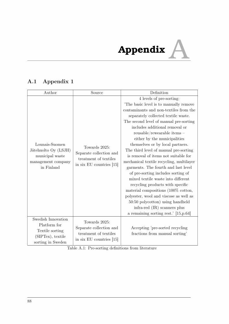
Appendix AA.1 Appendix 1

Author Source Definition

Lounais-SuomenJätehuolto Oy (LSJH)

municipal wastemanagement company

in Finland

Towards 2025:Separate collection andtreatment of textiles

in six EU countries [15]

4 levels of pre-sorting:’The basic level is to manually removecontaminants and non-textiles from the

separately collected textile waste.The second level of manual pre-sorting

includes additional removal orreusable/rewearable items –either by the municipalities

themselves or by local partners.The third level of manual pre-sortingis removal of items not suitable for

mechanical textile recycling, multilayergarments. The fourth and last levelof pre-sorting includes sorting ofmixed textile waste into differentrecycling products with specific

material compositions (100% cotton,polyester, wool and viscose as well as50:50 polycotton) using handheld

infra-red (IR) scanners plusa remaining sorting rest.’ [15,p.64]

Swedish InnovationPlatform forTextile sorting

(SIPTex), textilesorting in Sweden

Towards 2025:Separate collection andtreatment of textiles

in six EU countries [15]

Accepting ’pre-sorted recyclingfractions from manual sorting’

Table A.1: Pre-sorting definitions from literature

88

A.2. Appendix 2 AAU

A.2 Appendix 2

Table A.2: Weighted km per facility per region S3

Nordjylland Midtjylland Syddanmark Sjælland HovedstadenAalborg (N) 32.28 126.06 251.40 376.48 425.55Hjørring (N) 54.63 179.08 289.73 427.79 472.32

Frederikshavn (N) 67.71 189.05 314.40 439.98 488.59Århus (M) 138.36 51.50 140.57 265.98 311.98Randers (M) 100.86 64.25 171.44 296.98 345.56Viborg (M) 94.91 59.26 153.67 287.11 334.20Odense (Sd) 268.27 154.19 74.57 128.09 175.60Esbjerg (Sd) 280.23 142.32 96.49 258.06 306.79Vejle (Sd) 196.19 81.20 74.32 198.51 249.44

Roskilde (S) 396.42 281.11 198.96 42.77 42.64Næstved (S) 367.09 252.48 170.25 42.33 98.24Slagelse (S) 338.18 222.79 142.39 57.24 103.28Gladsaxe (H) 430.93 315.45 233.19 68.07 18.64Rudersdal (H) 442.42 301.04 244.65 79.43 23.47Helsingør (H) 467.25 351.82 269.62 104.35 43.98Trasborg (H) 402.27 298.17 217.35 50.54 33.64Red Cross (S) 391.03 275.68 194.44 42.46 50.74Red Cross (M) 177.88 69.60 96.68 222.44 265.14

Salvation Army (Sd) 210.07 101.60 59.15 185.73 235.38Salvation Army (H) 417.64 302.89 222.97 59.97 27.27

Table A.3: Variable cost per facility per region S3 [DKK/ton]

to / from Nordjylland Midtjylland Syddanmark Sjælland HovedstadenAalborg (N) 862.69 1,113.39 1,448.46 1,782.84 1,914.02Hjørring (N) 922.42 1,255.13 1,550.94 1,920.01 2,039.05

Frederikshavn (N) 957.40 1,281.77 1,616.88 1,952.58 2,082.54Århus (M) 1,169.44 937.24 1,175.35 1,510.58 1,633.57Randers (M) 1,069.19 971.30 1,257.85 1,593.46 1,723.35Viborg (M) 1,053.26 957.96 1,210.36 1,567.07 1,692.96Odense (Sd) 1,516.67 1,211.71 998.86 1,141.94 1,268.93Esbjerg (Sd) 1,548.64 1,179.96 1,057.45 1,489.38 1,619.64Vejle (Sd) 1,324.00 1,016.58 998.20 1,330.20 1,466.34

Roskilde (S) 1,977.10 1,668.84 1,449.23 1,031.68 1,031.32Næstved (S) 1,898.68 1,592.29 1,372.47 1,030.51 1,179.98Slagelse (S) 1,821.39 1,512.92 1,298.00 1,070.37 1,193.43Gladsaxe (H) 2,077.64 1,768.92 1,549.01 1,107.61 975.45Rudersdal (H) 2,108.37 1,730.40 1,579.65 1,137.98 988.38Helsingør (H) 2,174.74 1,866.15 1,646.42 1,204.60 1,043.22Trasborg (H) 2,001.03 1,722.75 1,506.69 1,060.75 1,015.57Red Cross (S) 1,962.67 1,654.32 1,437.13 1,030.86 1,052.99Red Cross (M) 1,275.08 985.62 1,057.99 1,394.19 1,508.35

Salvation Army (Sd) 1,361.09 1,071.12 957.65 1,296.03 1,428.74Salvation Army (H) 2,042.13 1,735.35 1,521.71 1,085.96 998.54

89

A. Appendix

Table A.4: Average renting cost per facility S3 [DKK/m2]

Facility PriceAalborg (N) 322Hjørring (N) 225

Frederikshavn (N) 200Århus (M) 493Randers (M) 400Viborg (M) 192Odense (Sd) 135Esbjerg (Sd) 345Vejle (Sd) 426

Roskilde (S) 400Næstved (S) 289Slagelse (S) 375Gladsaxe (H) 448Rudersdal (H) 531Helsingør (H) 600Trasborg (H) 400Red Cross (S) 439Red Cross (M) 365

Salvation Army (H) 597Salvation Army (Sd) 360

Table A.5: Fixed cost per facility per capacity option S3 [DKK/year]

to / from Low Low/medium Medium Medium/high HighAalborg (N) 56,350.00 295,903.13 535,456.26 775,009.39 1,014,562.52Hjørring (N) 39,375.00 206,764.61 374,154.22 541,543.83 708,933.44

Frederikshavn (N) 35,000.00 183,790.76 332,581.53 481,372.29 183,790.76Århus (M) 86,275.00 453,044.23 819,813.47 1,186,582.70 1,553,351.94Randers (M) 70,000.00 367,581.53 665,163.06 962,744.59 1,260,326.12Viborg (M) 33,600.00 176,439.13 319,278.27 462,117.40 604,956.54Odense (Sd) 23,625.00 124,058.77 224,492.53 324,926.30 425,360.06Esbjerg (Sd) 60,375.00 317,039.07 573,703.14 839,367.21 1,087,031.27Vejle (Sd) 74,550.00 391,474.33 708,398.66 1,025,322.98 1,342,247.31

Roskilde (S) 70,000.00 367,581.53 665,163.06 962,744.59 1,260,326.12Næstved (S) 50,575.00 265,577.65 480,580.31 695,582.96 910,585.62Slagelse (S) 65,625.00 344,607.68 623,590.37 902,573.05 1,181,555.73Gladsaxe (H) 78,400.00 411,691.31 744,982.62 1,078,273.94 1,411,565.25Rudersdal (H) 92,925.00 487,964.48 883,003.96 1,278,043.44 1,673,082.92Helsingør (H) 105,000.00 551,372.29 997,744.59 1,444,116.88 1,890,489.17Trasborg (H) 70,000 367,581.53 665,163.06 962,744.59 1,260,326.12RedCross (S) 76,825 403,420.73 730,016.46 1,056,612.18 1,383,207.91RedCross (M) 63,875 335,418.15 606,961.29 878,504.44 1,150,047.58

Salvation Army (Sd) 104,475 548,615.43 992,755.86 1,436,896.30 1,881,036.73Salvation Army (H) 63,000 330,823.38 598,646.75 866,470.13 1,134,293.50

90

a feasibility study of setting up a pre-sorting system for

Documents