1

CHARACTERIZATION AND ANALYSIS OF COW CREEK’S CONSTRUCTED RIPARIAN WETLAND

A. E. Kinsey, NSF REU Student, Auburn University; Dr. J.R. Vogel, Associate Professor, Extension Specialist, Oklahoma State University

Abstract

Constructed wetlands have been used to improve water quality, provide aquatic and riparian habitat, and as a means of flood control. Because it takes time for a wetland to adequately adapt, characterization of a newly constructed wetland should begin 3-5 years after construction is complete. The riparian constructed wetland in the Oklahoma State University Botanical Gardens was completed in 2012. Its main influent source was a nearby water treatment plant’s lagoon effluent. An ADCP bathymetry test revealed that the volume was 22,281 ft3. The hydraulic retention time (HRT) peak was determined from a rhodamine dye tracer study to be 1 day, with 50% of the rhodamine dye recovered after 2.41 days. A double peak in the tracer response curve revealed the break in flow of the inlet lagoon effluent from the pipe to the back of the wetland. Though the wetland inlet did not have detectable orthophosphate levels, the wetland’s average nutrient removal efficiency for nitrate was 65%. Tests showed that the wetland is sufficient at removing low-level nitrates with a short HRT. Further characterization tests in the future could include plant and macro invertebrate species identification, California Rapid Assessment Method for riparian wetlands, analysis of hydraulic dead zones, and an expended storm event study. Keywords: constructed wetland, bathymetry, hydraulic retention time, rhodamine, nutrient removal Introduction

Natural wetlands provide crucial ecosystem services such as improving water quality through nutrient removal, providing aquatic and riparian habitat, and flood control. Recently, constructed wetlands have been designed and constructed in order to provide these services in a more controlled way or in locations where they were not naturally occurring. Constructed wetlands attempt to mimic their natural counterparts in ecosystem services and can have the added advantage of being optimized for a specific function. Constructed wetlands less than two years old cannot be accurately characterized for water quality due to their lack of adaptation (Kadlec & Wallace, 2009). Because of this, it is recommended to begin accurately testing for efficiency 5-15 years after construction.

Constructed wetlands are usually characterized into two main types: subsurface flow (SSF) and free water surface (FWS) flow. SSF constructed wetlands are designed with the intentions of treating water in gravel media and roots, while FWS constructed wetlands more mimic natural wetlands by utilizing open water pools and its flora and fauna. Many wetlands are constructed and research is conducted for the purpose of optimizing nutrient reduction, especially the various forms of nitrogen and

2

phosphorus, which are major contributors to eutrophication (Appelboom, Engineer, Ave, Rouge, & Fouss, 2006; Giacalone, Obropta, & Miskewitz, 2007; Gottschall, Boutin, Crolla, Kinsley, & Champagne, 2007; Iamchaturapatr, Yi, & Rhee, 2007; La Flamme, Enright, & Madramootoo, 2004; Vymazal, 2005, 2007).

In order for a constructed wetland to be successful at removing total nitrogen it must have multiple depth stages (Mihelcic & Zimmerman, 2014). These different stages create the aerobic and anaerobic conditions needed for the complex nitrogen cycle. A shallow zone of one foot or less creates anaerobic conditions needed for ammonification and nitrification, and deeper zones of 3-5 feet create aerobic conditions for denitrification (Mihelcic & Zimmerman, 2014). While nitrogen is removed through the denitrification process, phosphorus is mainly removed through sorption into the soil and plant uptake (Huffman, Fangmeier, Elliot, & Workman, 2013; Vymazal, 2007). Orthophosphate (ortho-P) is the form that is taken up and used by plants and algae. Removal of phosphorus in literature is found to be low unless specific plant species or soil types are selected in the design (Vymazal, 2007).

The varying cell depths and flow rate of a wetland affect the hydraulic retention time (HRT) of the wetland, or how long a parcel of water stays in the wetland, and thus affects the effluent water quality (Hunt, 2002). When a wetland’s purpose is to reduce pathogens, the optimum HRT is 10 or greater in order to ensure that the pathogens are reduced naturally or by sunlight (Tousignant, Fankhauser, & Hurd, 1999). While most wetlands are designed using plug-flow reactor (PFR) concepts, in actuality wetlands function as a mixture between PFR and continuously stirred tank reactor (CSTR) due to stagnant regions or preferential flow paths (Hunt, 2002). A common method for determining the HRT of a stream or wetland is to perform a dye tracer test in which a conservative dye is injected into the system. Graphing the dye’s concentration downstream over time creates a tracer response curve, which creates a peak HRT.

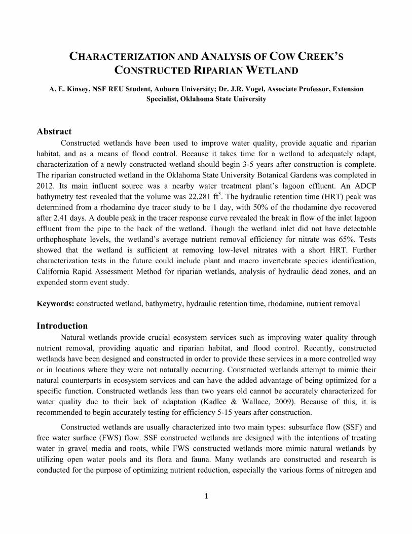
In 2011, Oklahoma State University (OSU) initiated a project involving the construction of a riparian wetland and stabilization of a meander bend of Cow Creek located in the OSU Botanical Gardens in Stillwater, Oklahoma. The initial design of the Cow Creek constructed wetland was to receive runoff from the OSU Agronomy farm adjacent to the wetland and effluent from the nearby water treatment plant (WTP) lagoon (Maronek, Fox, Lovern, Chavez, & Miller, 2012). However, agricultural runoff into the wetland only primarily occurred after large storm events, leaving the lagoon effluent to be the main continuous source of inflow. The constructed wetland received a portion of the effluent, while the rest flowed into Cow Creek just before the meander that surrounded the wetland. Design blueprints showed a surface area of around 61,000 square feet, with a 5-feet deep pool near the outlet and areas that varied from 0-4 feet (Maronek et al., 2012). Figure 1 shows the design layout of the Cow Creek stream rehabilitation project and constructed wetland.

3

Objective/Hypothesis

The goal of this project was to determine how the Cow Creek constructed wetland was functioning in terms of water quality reduction. Because the wetland had not been characterized or observed since the completion of its construction in 2012, the objectives of this project were to characterize it by means of defining the current volume of the wetland, determining the travel time of a parcel of water through the wetland, and discuss concentration reductions of various water quality parameters between the inlet and the outlet of the wetland.

Past research suggested that FWS wetlands of similar structure had an average HRT of 8.1 days (Huffman et al., 2013; Hunt, 2002). A manual created by the University of Guelph gave the following equation for estimating the HRT of a FWS constructed wetland (Tousignant et al., 1999):

𝐻𝑅𝑇 = 𝑉𝑄 ×

0.9560 ×60 ×24

where:

HRT = hydraulic retention time (days) V = volume of wetland (ft3) Q = discharge at wetland outlet (cfs)

This equation estimated the HRT of the Cow Creek constructed wetland to be 5 days.

Based on previous literature of FWS constructed wetland research, the mean removal of nitrate was 42.4% (Valsero et al, 2012; Vymazal, 2007) and the mean ortho-P removal was 44.1% (Hijosa-Valsero et al., 2012; La Flamme et al., 2004). If the constructed wetland had sufficient depths and plant species, then it was estimated that there would be a decrease in nutrients from the inlet to outlet.

(1)

Figure 1: Design blueprints for the Cow Creek stream stabilization and constructed wetland project. Left: Cow Creek design blueprint. Right: Riparian constructed wetland design blueprint. (Karns, 2012)

4

Methods 1. Bathymetry An acoustic Doppler current profiler (ADCP) was used to determine the depths at various points of the wetland. At each of the nineteen cross sections seen in figure 2, the ADCP boat was pulled across the wetland two times in order to gather accurate latitude, longitude, and depth points. These points were used in a MATLAB code (appendix 1) created by Alex McLemore, an Oklahoma State University PhD student, to graph the points into 3D models of the constructed wetland and calculate the area under that graph, or the current wetland volume.

2. Travel Time The travel time of a parcel of water was determined two ways: dividing current wetland volume by outlet discharge and conducting a rhodamine dye tracer study on the wetland. The minimum, maximum, mean, and quartile values of the outlet discharge data collected over the course of the two-month study was used with the current wetland volume determined by the ADCP bathymetry procedure to calculate the corresponding statistical travel times.

Methods similar to the single slug and grab sampling methods outlined by Kitpatrick & Wilson (1989) for the USGS were used for this research. Rhodamine, a fluorescent dye typically used in tracer studies, was chosen for this study because it resisted absorption and was detectable in low

Figure 2: Sketch of constructed wetland and cross sections where ADCP boat was pulled across the wetland to acquire latitude, longitude, and depth points.

5

concentrations. Also, it was not harmful to the environment because of its light sensitivity and eventual degradation over time. Because the dye was injected at the only inlet point of the wetland, it was believed to be well mixed throughout the system during the test. The amount of rhodamine needed for a common peak concentration of 20 ppb was calculated from equation 2, and was found to be 63 g of 20% stock rhodamine.

𝑉! =𝑉×𝐶!0.2

where:

Vs = volume of 20% stock rhodamine (L) V = volume of wetland (L) Cp

= peak concentration at outlet sampling site (ppb)

This value was doubled and rounded to 130 g of 20% stock rhodamine in order to account for underestimation errors in the volume calculated from the ADCP bathymetry study and for the dye sticking to organic matter. The dye was injected into outlet flow of the pipe from the WTP that empties into the wetland in order to ensure rapid, complete mixing, and the start time was recorded. Because there was only a single point at the outlet of the wetland that emptied into Cow Creek, only one monitoring site was needed. An initial water sample was collected at the outlet in order to establish a base fluorescence reading. A Trilogy ® Laboratory Fluorometer was used to measure the fluorescence level of each outlet water sample, collected by an ISCO 6712 Autosampler. The wetland outlet was monitored and water samples were taken every 3 hours until the fluorescence increased more rapidly. At which point, samples were taken every 30 minutes so as not to miss the curve’s peak. When the fluorescence began to decrease more gradually, sampling intervals were shorted to 1 hour, then 2 hours, and later back to 3 hours until the fluorescence matched the original base level.

A third set of statistical travel times was calculated using the current volume and outlet flows measured during the rhodamine study. These times were then compared to the times determined from the rhodamine study.

3. Nutrient Removal ISCO 6712 autosamplers on the inlet and outlet of the wetland were used to collect samples every three hours for two days for multiple test sets. Samples were collected during base flow, which was defined as an average, constant flow not during or recently after a storm event. A 45˚ v-notch weir on the inlet pipe and a 120˚ v-notch weir on the outlet of the wetland were used in combination with ISCO 720 submerged pressure transducer to measure flow rate on the wetland’s inlet and outlet. An ISCO 674 Rain Gauge by the inlet autosampler collected rain level data during sampling. Discharge, Q (cfs), was calculated from head on the weir, H, in feet and weir type by the following ISCO equations (Teledyne Isco Open Channel Flow Measurement Handbook, 2013):

(2)

6

For 120˚ v-notch weir:

𝑄 = 4.33𝐻!.! For 45˚ v-notch weir:

𝑄 = 1.035𝐻!.! Each water sample was analyzed for NO3

-, ortho-P, Cl-, SO42-, pH, conductivity, and turbidity in

Oklahoma State University’s Soil, Water, and Forage Analytical laboratory. Statistical data was calculated for the various inlet and outlet parameters, including mean, median, minimum value, maximum value, and 1st and 3rd quartiles. In order to determine correlation and significance, a correlation matrix containing R2 values and P-values was made using Minitab. Results & Discussion 1. Bathymetry The MATLAB code imported the Excel files containing the latitude, longitude, and depth points from the ADCP and were graphed into 3D models of the constructed wetland (figures 3a & 3b).

The MATLAB program also calculated the volume, or area under the curve, of the wetland to be 21,220 ft3. Because the ADCP boat could not measure depths under floating obstructions, such as lily pads, 5% was added to the calculated volume bringing it to 22,300 ft3. 5% was chosen because it was visually estimated that 5% of the wetland was covered by obstructions. Using the graphical interpretation of the constructed wetland, the largest width was 121.4 feet and the longest length was 235.5 feet. Assuming a rectangular wetland shape, the calculated area was 28,590 square feet, or 53%

Depth(ft)

Longitude

Latitude

Depth(ft)

Latitude

Longitude

(a) (b)

Figure 3: (a) 3D view of the depth of the constructed wetland (b) 2D model with a depth color gradient showing depth by color scale of the constructed wetland

(3)

(4)

7

smaller than the design area of 61,000 ft2 stated in the Cow Creek final report (Maronek et al., 2012). Errors in the wetland design could have come from an overestimation of inlet flow to the wetland, which would cause the actual surface area of the wetland to be smaller than the design surface area.

2.Timeoftravel

The current wetland volume was used with the outlet discharges from the duration of the two-month study to find statistic travel time of a parcel of water (table 1a). The maximum time was 12.72 days, and the average time was 3.45 days. These values represent travel times for a broad range of data over two months. Using the average outlet flow during the tracer dye study of 0.09162 cfs and the mean HRT of 2.41 days, an approximate volume was calculated to be 19,318 ft3. This was only 13% percent different than the volume found from the ADCP bathymetry test, confirming the measured volume of the constructed wetland.

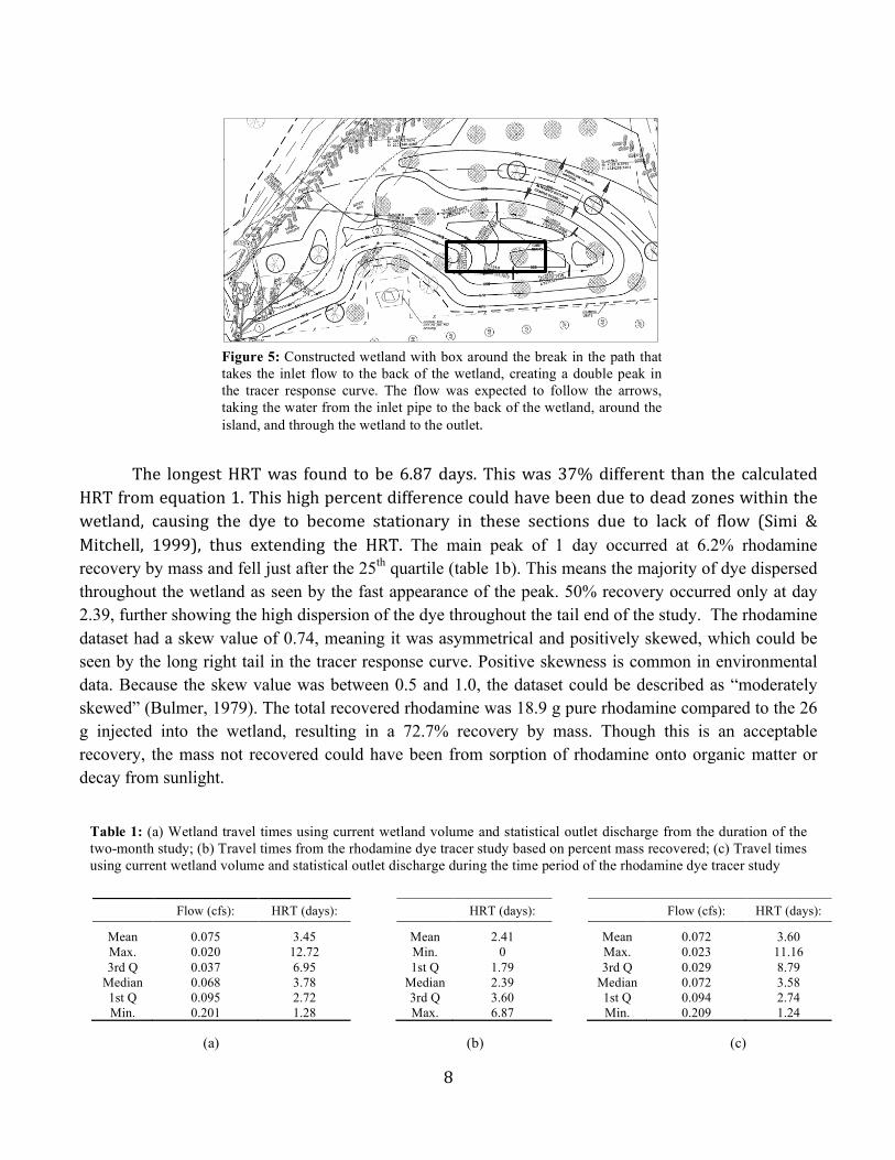
A graph of rhodamine concentration vs. time was created to establish a tracer response curve (figure 4). The curve showed two peaks, the first at 0.25 days and the second at 1.00 days. According to Hunt (2002), two peaks is a sign that two flow paths are present, with the first peak being the shorter flow path. The two peaks found were representative of the wetland’s design, as there was a break in the inlet flow path that takes the flow from the inlet pipe to the back of the wetland (figure 5). This allowed a portion of the dye to reach the outlet faster, causing the double peak in the tracer response curve.

Figure 4: Tracer response curve with peaks at 0.25 days and 1.00 days

0.00

0.05

0.10

0.15

0.20

0.25

051015202530354045

0 1 2 3 4 5 6 7

Out

let d

isch

arge

(cfs

)

Rho

dam

ine

Con

cent

ratio

n (p

pb)

Time (days)

Tracerresponsecurve Outletdischarge

8

The longestHRTwas found to be6.87days. Thiswas37%different than the calculatedHRTfromequation1.Thishighpercentdifferencecouldhavebeenduetodeadzoneswithinthewetland, causing the dye to become stationary in these sections due to lack of flow (Simi &Mitchell, 1999), thus extending the HRT. The main peak of 1 day occurred at 6.2% rhodamine recovery by mass and fell just after the 25th quartile (table 1b). This means the majority of dye dispersed throughout the wetland as seen by the fast appearance of the peak. 50% recovery occurred only at day 2.39, further showing the high dispersion of the dye throughout the tail end of the study. The rhodamine dataset had a skew value of 0.74, meaning it was asymmetrical and positively skewed, which could be seen by the long right tail in the tracer response curve. Positive skewness is common in environmental data. Because the skew value was between 0.5 and 1.0, the dataset could be described as “moderately skewed” (Bulmer, 1979). The total recovered rhodamine was 18.9 g pure rhodamine compared to the 26 g injected into the wetland, resulting in a 72.7% recovery by mass. Though this is an acceptable recovery, the mass not recovered could have been from sorption of rhodamine onto organic matter or decay from sunlight.

Flow (cfs): HRT (days): HRT (days): Flow (cfs): HRT (days):

Mean 0.075 3.45

Mean 2.41

Mean 0.072 3.60 Max. 0.020 12.72

Min. 0

Max. 0.023 11.16

3rd Q 0.037 6.95

1st Q 1.79

3rd Q 0.029 8.79 Median 0.068 3.78

Median 2.39

Median 0.072 3.58

1st Q 0.095 2.72

3rd Q 3.60

1st Q 0.094 2.74 Min. 0.201 1.28

Max. 6.87

Min. 0.209 1.24

Table 1: (a) Wetland travel times using current wetland volume and statistical outlet discharge from the duration of the two-month study; (b) Travel times from the rhodamine dye tracer study based on percent mass recovered; (c) Travel times using current wetland volume and statistical outlet discharge during the time period of the rhodamine dye tracer study

Figure 5: Constructed wetland with box around the break in the path that takes the inlet flow to the back of the wetland, creating a double peak in the tracer response curve. The flow was expected to follow the arrows, taking the water from the inlet pipe to the back of the wetland, around the island, and through the wetland to the outlet.

(a) (b) (c)

9

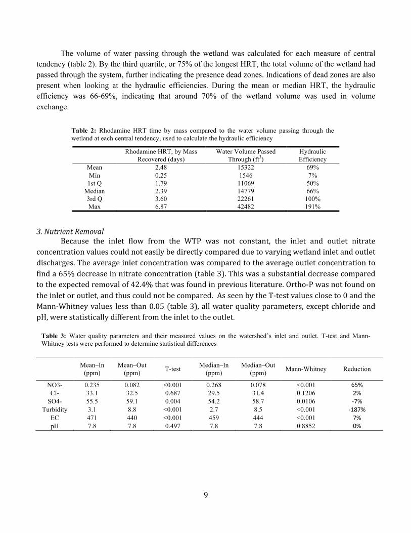
The volume of water passing through the wetland was calculated for each measure of central tendency (table 2). By the third quartile, or 75% of the longest HRT, the total volume of the wetland had passed through the system, further indicating the presence dead zones. Indications of dead zones are also present when looking at the hydraulic efficiencies. During the mean or median HRT, the hydraulic efficiency was 66-69%, indicating that around 70% of the wetland volume was used in volume exchange.

Rhodamine HRT, by Mass

Recovered (days) Water Volume Passed

Through (ft3) Hydraulic Efficiency

Mean 2.48 15322 69% Min 0.25 1546 7% 1st Q 1.79 11069 50%

Median 2.39 14779 66% 3rd Q 3.60 22261 100% Max 6.87 42482 191%

3.NutrientRemovalBecause the inlet flow from the WTP was not constant, the inlet and outlet nitrate

concentrationvaluescouldnoteasilybedirectlycomparedduetovaryingwetlandinletandoutletdischarges.Theaverageinletconcentrationwascomparedtotheaverageoutletconcentrationtofinda65%decreaseinnitrateconcentration(table3).Thiswasasubstantialdecreasecomparedtotheexpectedremovalof42.4%thatwasfoundinpreviousliterature.Ortho-Pwasnotfoundontheinletoroutlet,andthuscouldnotbecompared.AsseenbytheT-testvaluescloseto0andtheMann-Whitneyvalues less than0.05(table3),allwaterqualityparameters,exceptchlorideandpH,werestatisticallydifferentfromtheinlettotheoutlet.

Mean–In (ppm)

Mean–Out (ppm) T-test Median–In

(ppm) Median–Out

(ppm) Mann-Whitney Reduction

NO3- 0.235 0.082 <0.001 0.268 0.078 <0.001 65%Cl- 33.1 32.5 0.687 29.5 31.4 0.1206 2%

SO4- 55.5 59.1 0.004 54.2 58.7 0.0106 -7%Turbidity 3.1 8.8 <0.001 2.7 8.5 <0.001 -187%

EC 471 440 <0.001 459 444 <0.001 7%pH 7.8 7.8 0.497 7.8 7.8 0.8852 0%

Table 2: Rhodamine HRT time by mass compared to the water volume passing through the wetland at each central tendency, used to calculate the hydraulic efficiency

Table 3: Water quality parameters and their measured values on the watershed’s inlet and outlet. T-test and Mann-Whitney tests were performed to determine statistical differences

10

Onaverage,nitrateswerefoundtodecreasefrominlettooutlet.Sulfate isaconservativeparameter,buttheaveragemeansstatisticallydifferandincreasefrominlettooutlet.Thisisdueto sulfur’s involvement in the complex nitrogen cycle. It is a product of nitrogen reduction inanaerobic conditions. To confirm this, a correlation analysiswas performedon all of thewaterquality parameters (table 4). Sulfate was strongly negatively correlated to nitrate, a furtherindication of sulfate as a product of the nitrogen cycle. Additionally, electroconductivity wasstrongly positively correlated to chlorides, which can be explained by chlorides causing highsalinity,andthushighelectroconductivity.

N-In

(ppm) Cl-In (ppm)

SO4-In (ppm)

Turb-In (NTU)

EC-In (uS/cm)

Cl-In (ppm) 0.21 1.00

0.166

SO4-In (ppm) -0.78 -0.46 1.00

<0.001 <0.001

Turb.-In (NTU) 0.62 0.39 -0.53 1

<0.001 0.010 <0.001

EC-In (uS/cm) 0.21 0.94 -0.34 0.44 1.00

0.172 <0.001 0.025 0.003

pH-In -0.69 -0.01 0.41 -0.47 0.02 <0.001 0.959 0.006 0.001 0.915

(a)

N-Out (ppm)

Cl-Out (ppm)

SO4-Out (ppm)

Turb-Out (NTU)

EC-Out (uS/cm)

Cl-Out (ppm) 0.63 1.00

<0.001

SO4-Out (ppm) -0.80 -0.51 1.00

<0.001 <0.001

Turb.-Out (NTU) -0.31 -0.54 0.27 1

0.041 <0.001 0.072

EC-Out (uS/cm) 0.26 0.60 0.14 -0.38 1.00

0.084 <0.001 0.379 0.010

pH-Out 0.54 0.56 -0.51 -0.61 0.22 <0.001 <0.001 <0.001 <0.001 0.160

(b)

Table 4: Correlation analysis between all water quality parameters on the inlet (a) and outlet (b) of the watershed

11

Conclusions Cow Creek’s constructed riparian wetland was characterized and analyzed based on volume,

HRT, and nutrient removal. Through the use of an ADCP, a 3D model of the wetland was created and integrated to calculate the volume. Adding 5% to the volume for ADCP obstructions revealed that the wetland’s volume was 22,300 ft3, resulting in roughly half the area of the design blueprints. Through a dye tracer study, the longest time a parcel of water stayed in the wetland was 6.87 days. The tracer response curve revealed peaks at 0.25 days and 1.00 days, indicating short-circuiting in the wetland’s design.

Cow Creek’s constructed riparian wetland was found to be a well-functioning wetland, especially for removal of nitrates and for flood control. In order to expand on its characterization, future research could include identification of plants and macro invertebrates within the wetland and how they relate to its efficiency and health, the California Rapid Assessment Method for riparian wetlands to further assess the wetland’s performance and its surroundings, analysis of the hydraulic dead zones within the wetland to better explain why the HRT was longer than expected, and an extended storm study to expand on the wetland’s abilities for flood control.

Acknowledgements

The authors acknowledge the financial support provided by the National Science Foundation through award number EAR1358908 titled “REU Site: Evaluating the Effectiveness of Stream Restoration Projects Based on Natural Channel Design Concepts Using Process-Based Investigations”. The authors also acknowledge Alex McLemore, John McMaine, Yan “Joey” Zhou, Dr. Ron Miller, and Dr. Luci Guertault for their assistance with the research. References Appelboom, T. W., Engineer, A., Ave, G., Rouge, B., & Fouss, J. L. (2006). Methods for Removing

Nitrate Nitrogen from Agricultural Drainage Waters. Society, 0300(06). Bulmer, M. G. (1979). Principles of Statistics. New York: Dover Publications. Giacalone, K. A., Obropta, C. C., & Miskewitz, R. J. (2007). Use of vegetation to mitigate nutrient

discharges in container nursery runoff, 50(5), 1517–1523. Gottschall, N., Boutin, C., Crolla, A., Kinsley, C., & Champagne, P. (2007). The role of plants in the

removal of nutrients at a constructed wetland treating agricultural (dairy) wastewater, Ontario, Canada. Ecological Engineering. http://doi.org/10.1016/j.ecoleng.2006.06.004

Hijosa-Valsero, M., Sidrach-Cardona, R., & Bécares, E. (2012). Comparison of interannual removal variation of various constructed wetland types. Science of the Total Environment. http://doi.org/10.1016/j.scitotenv.2012.04.072

Huffman, R. L., Fangmeier, D. D., Elliot, W. J., & Workman, S. R. (Eds.). (2013). Soil and Water Conservation Engineering (7th ed.). ASABE.

Hunt, B. (2002). Determining the actual hydraulic retention time of a constructed wetland cell for comparison with the theoretical hydraulic retention time.

12

Iamchaturapatr, J., Yi, S. W., & Rhee, J. S. (2007). Nutrient removals by 21 aquatic plants for vertical free surface-flow (VFS) constructed wetland. Ecological Engineering. http://doi.org/10.1016/j.ecoleng.2006.09.010

Kadlec, R. H., & Wallace, S. D. (Eds.). (2009). Treatment Wetlands (2nd ed.). New York: Taylor & Francis Group, LLC.

Karns, M. (2012). Plan of Proposed Cow Creek Channel Stabilization & Restoration. Tulsa, OK: Cobb Engineering Company.

La Flamme, C., Enright, P., & Madramootoo, C. (2004). Sediment and Nutrient Removal Efficiencies in a Constructed Wetland in Southern Quebec. ASABE.

Maronek, D., Fox, G., Lovern, S., Chavez, R., & Miller, R. (2012). Cow Creek Stream Restoration and Streambank Stabilization Project.

Mihelcic, J. R., & Zimmerman, J. B. (Eds.). (2014). Environmental Engineering: Fundamentals, sustainability, design (2nd ed.). John Wiley & Sons, Inc.

Simi, A. L., & Mitchell, C. A. (1999). Design and hydraulic performance of a constructed wetland treating oil refinery wastewater. Water Science and Technology, 40(3), 301–307.

Teledyne Isco Open Channel Flow Measurement Handbook. (2013) (7th ed.). Lincoln: Teledyne Technologies, Inc.

Tousignant, E., Fankhauser, O., & Hurd, S. (1999). Guidance manual for the design, construction and operations of constructed wetlands for rural applications in Ontario. Retrieved from http://agrienvarchive.ca/bioenergy/download/wetlands_manual.pdf

Vymazal, J. (2005). Horizontal sub-surface flow and hybrid constructed wetlands systems for wastewater treatment. In Ecological Engineering. http://doi.org/10.1016/j.ecoleng.2005.07.010

Vymazal, J. (2007). Removal of nutrients in various types of constructed wetlands. Science of the Total Environment. http://doi.org/10.1016/j.scitotenv.2006.09.014

13

Appendix Appendix 1: MATLAB Code for total wetland volume % Alex McLemore 10/28/2014 % script to develop stage-volume relationship from set of points (x,y,z) % note: survey data points are inported as invertered values (i.e. % upsidedown) clc clear filename = 'alldata.xlsx'; sheet = 'alldata'; x1Range = 'A3:H5362'; data_points=xlsread(filename,sheet,x1Range); UTMx = data_points(:,6); %length along cell (north to south) (ft) UTMy = data_points(:,7); %width along cell (east to west) (ft) h = data_points(:,3); %elevation (ft) x = UTMx-min(UTMx); y = UTMy-min(UTMy); %plot3(h,x,y,'linestyle','none','marker','.') [cell_surf,gof] = fit([x,y],h,'linearinterp'); %creating fit equation plot(cell_surf,'Style','surface') %for visual confirmation res = 0.05; %grid resolution (m), must be less than smallest survey length [xg,yg] = meshgrid(0:res:max(x),0:res:max(y)); %creating high res grid of x,y points zg = cell_surf(xg,yg); %solving z for high res grid of x,y points %z_flood = 1; %max elevation before flooding begins %z_max = max(max(zg)); %used to removing flood elevations %zg = zg-(z_max-z_flood); %makes area above flood stage become negative zg(isnan(zg))=0; %replacing NAN with 0 %zg(zg<0)=0; %replacing values above floodplain to zero surf(xg,yg,zg,'linestyle','none') % total volume volume = res*res*trapz(trapz(zg)); % process to create stage-volume relationship %{ step = 0.01; stage = (0:step:max(h)); for i = 1:length(stage) cuml_vol(i) = res*res*trapz(trapz(zg)); % double numercial integration of cell surf zg = zg-step; %shifting cell surf down 1 stage increment zg(zg<0) = 0; %changing negative values to 0 %plot_surf(:,:,i) = zg.*(-1); %surf(xg,yg,plot_surf(:,:,i)) %plot cell surface %hold on end %hold off stage = stage'; cuml_vol = flipud(cuml_vol'); [SD,gof2] = fit(stage,cuml_vol,'poly4') hold on

14

plot(stage,cuml_vol) plot(SD) hold off %} % commands to create 3D printer files % FV = surf2solid(xg,yg,zg.*25,'elevation',min(zg(:))-0.05); stlwrite('BGwetland.stl', FV) %FV2 = surf2solid(xg,yg,cell_surf_hires.*25,'thickness',-0.5); %stlwrite('green_swing_cubic_shell.stl', FV2) %figure %subplot(1,1,1), title 'Thin surface' %surf2solid(xg,yg,cell_surf_hires.*25,'elevation',min(cell_surf_hires(:))-0.05); %