CAEPR Working Paper #2015-002

A Divide and Conquer Algorithm for Exploiting Policy Function Monotonicity

Grey Gordon and Shi Qiu

Indiana University, United States of America

January 27, 2015

This paper can be downloaded without charge from the Social Science Research Network electronic library at http://ssrn.com/abstract=2556345

The Center for Applied Economics and Policy Research resides in the Department of Economics at Indiana University Bloomington. CAEPR can be found on the Internet at: http://www.indiana.edu/~caepr. CAEPR can be reached via email at caepr@indiana.edu or via phone at 812-855-4050.

©2015 by Grey Gordon and Shi Qiu. All rights reserved. Short sections of text, not to exceed two paragraphs, may be quoted without explicit permission provided that full credit, including © notice, is given to the source.

A Divide and Conquer Algorithm for Exploiting Policy

Function Monotonicity

Grey Gordon and Shi Qiu

January 27, 2015

Abstract

A divide-and-conquer algorithm for exploiting policy function monotonicity is pro-

posed and analyzed. To compute a discrete problem with n states and n choices, the

algorithm requires at most 5n+ log2(n)n function evaluations and so is O(n log2 n). In

contrast, existing methods for non-concave problems require n2 evaluations in the worst-

case and so are O(n2). The algorithm holds great promise for discrete choice models

where non-concavities naturally arise. In one such example, the sovereign default model

of Arellano (2008), the algorithm is six times faster than the best existing method when

n = 100 and 50 times faster when n = 1000. Moreover, if concavity is assumed, the

algorithm combined with Heer and Maußner (2005)’s method requires fewer than 18n

evaluations and so is O(n).

1 Introduction

Monotone policy functions arise naturally in economic models.1 In this paper, we provide a

computational algorithm, which we refer to as “binary monotonicity,” that exploits policy

function monotonicity using a divide and conquer algorithm. Our focus is on problems of

the following form:

Π(i) = maxi′∈{1,...,n′}

π(i, i′) (1)

for i ∈ {1, . . . , n} with an associated optimal policy g. While this is abstract, economic

problems of this form abound. For example, consider the two period utility maximization

problem V (b, y) = maxb′∈B log(−b′ + b + y) + log(b′) where b and b′ are some measure of

savings constrained to lie in a grid B, y is an endowment, and log(·) is the period utility

1For example, one of the most common state and choice variables is some measure of savings. It is thenquite natural for the model to predict that wealthier agents save more in levels else equal, which resultsin a savings policy that is monotonically increasing in wealth. This is the case for the real business cyclemodel, the standard incomplete markets models of Aiyagari (1994) and Krusell and Smith (1998), the defaultmodels of Arellano (2008) and Chatterjee, Corbae, Nakajima, and Rıos-Rull (2007), and many others.

1

function. Letting Bj denote the jth element of the grid, one can create a separate problem for

each y with Πy(i) = maxi′∈{1,...,#B} πy(i, i′) and πy(i, i

′) = log(−Bi′+Bi+y)+log(Bi′). In this

case, one has V (Bi, y) = Πy(i).2 Beyond this simple example, we show how the standard

real business cycle model (with leisure) and Arellano (2008)’s model can be cast in this

form. Letting an optimal policy associated with (1) be denoted g, we say g is monotonically

increasing if g(i) ≤ g(j) whenever i ≤ j. We restrict attention to monotonically increasing

policies, but our results extend naturally to monotonically decreasing policies. Our method

exploits monotonicity to solve (1) in no more than 3n′ + 2n+ log2(n)n′ evaluations of π.

While concavity also arises naturally in economic models, for certain classes of models,

it does not. Discrete choice models are the foremost example. In them, the value function

is the upper envelope of a finite number of “subsidiary” value functions conditional on

the discrete choice. Even if the subsidiary value functions are concave, the upper envelope

is generally not. For instance, in the Arellano (2008) model we consider in this paper,

the value function for an indebted sovereign (for whom it is refeasible to repay debt) is

V (b, y) = maxd∈{0,1} dVd(y) + (1 − d)V nd(b, y) where b is a sovereign’s bond position, y is

output, d is the default decision, V d(y) is the value conditional on default, and V nd(b, y)

is the value conditional on repaying. In this case, even if the subsidiary value functions V d

and V nd are concave in b, V is not.3

Within the classes of models where monotonicity obtains but concavity does not, few

computational options are available. Many of the fastest and most accurate methods, such

as projection and Carroll (2006)’s endogenous gridpoints method (EGM), work with first

order conditions (FOCs). Similarly, linearization and higher-order perturbations (which are

less accurate but even faster) also work with FOCs. However, without concavity, FOCs are

necessary but not sufficient, and so one cannot rely on FOC methods alone as there may be

multiple local maxima. This also makes the use of any direct maximization routines over a

continuous search space (perhaps the most common being the simplex method) dangerous.

Because of these problems, grid search is often used for non-concave problems.4

For solving a non-concave problem via grid search, we are aware of only two existing

methods. The first, which we refer to as “brute force,” evaluates π for every possible (i, i′)

combination. The second, which we refer to as “simple monotonicity,” uses monotonicity to

restrict the search space for g(i) to {g(i − 1), . . . , n′} when i > 1. Our method dominates

2Of course, not every i′ may be feasible, and whether a given i′ is feasible depends on i (and y). In Section2.1 and Appendix B, we show how the results generalize to a problem where the feasible choice set is notnecessarily fixed. Note also that, since the choice set is not convex, the problem (1) may have more than oneoptimal policy. We discuss this issue more in Section 2.1.

3Using the convention −b is a sovereign’s debt, for a b∗ such that the sovereign is indifferent betweendefault and repayment, i.e. V d(y) = V nd(b∗, y), one has V (b∗− ε, y) = V (b∗, y) < V (b∗+ ε, y) for any ε > 0.Hence, V is not concave at b∗.

4Even if one ultimately solves a continuous problem, a grid search is often done as a first step to avoidlocal minima.

2

these in terms of worst-case behavior where both brute force and simple monotonicity

require nn′ evaluations.5 While the worst case behavior for simple monotonicity could be

misleading, we find practically that it is not: For both the RBC model and Arellano (2008)

model, simple monotonicity uses roughly .4nn′ to .5nn′ evaluations for many different values

of n and n′. In contrast, our method requires at most 3n′ + 2n + log2(n)n′ evaluations in

the worst case. This makes binary monotonicity faster for small n and n′ and exponentially

faster as n and n′ become large.

Our method, which we refer to as “binary monotonicity,” achieves this by using a divide

and conquer algorithm. A brief description of it is as follows with a complete description

given in Section 2.3. The algorithm initially computes g(1) and g(n), essentially by brute

force, and defines i = 1 and i = n. The core of the algorithm assumes g(i) and g(i) are known

and computes the optimum for all i ∈ {i, . . . , i} recursively. Definingm = b(i+i)/2c, it solves

for g(m). Because of monotonicity, g(m)—which in general might be any of {1, . . . , n′}—must lie in {g(i), . . . , g(i)}. With g(m) computed, the algorithm then recursively proceeds

to the core of the algorithm twice, once for (i, i) redefined to be (i,m) and once for (i, i)

redefined to be (m, i). The recursion stops when i ≤ i + 1, since then g is known for all

i ∈ {i, . . . , i}.To assess our method for real-life cases, we consider two common economic environ-

ments. The first environment we consider is the sovereign default model of Arellano (2008).

For this model, the sovereign’s savings policy is substantially non-linear. The second en-

vironment we consider is the real business cycle (RBC) model. For this model, it is well

known that the capital policy is nearly linear in capital holdings. For both these models, we

find simple monotonicity is roughly twice as fast as brute force. In contrast, we find that

binary monotonicity is roughly six, 50, and 400 times faster than simple monotonicity for

grid sizes of 100, 1000, and 10000 points, respectively.

For the RBC model, we can combine brute force, simple monotonicity, and binary mono-

tonicity with techniques that exploit concavity.6 We are aware of two methods that exploit

concavity to solve for maxi′∈{a,...,b} π(i, i′) in possibly fewer than b− a+ 1 evaluations. The

first, which we refer to as “simple concavity,” iterates through the list a, a+ 1, . . . and stops

whenever π(i, i′) falls. The second, which we refer to as “binary concavity,” is the method

of Heer and Maußner (2005).7 This approach uses divide and conquer, evaluating π(i, i′) at

i′ = m := b(a + b)/2c and m + 1, and subsequently restricting the {a, . . . , b} search space

to either {a, . . . ,m} or {m+ 1, . . . , b}.5The worst case behavior for simple monotonicity obtains when the true policy is g(·) = 1.6Throughout the paper, we say the algorithms exploit concavity. However, the algorithms actually exploit

something closer to quasi-concavity. See Appendix B, Section B.2, for details.7Their algorithm in its original form can be found on p. 26 of Heer and Maußner (2005). Our implemen-

tation, given in Appendix A, differs slightly.

3

We prove that if the problem is concave, binary monotonicity can be combined with

binary concavity to solve (1) in no more than 8n′ + 10n evaluations of π in the worst case,

a striking result. Surprisingly, however, for the RBC model with a linearly spaced capital

grid we find that binary concavity with binary monotonicity is the second fastest approach.

Simple concavity with simple monotonicity ends up faster because the optimal policy very

nearly satisfies g(i + 1) = g(i) + 1 and, for a given i, only three π evaluations to compute

the optimum in this case.8 We find binary monotonicity with binary concavity takes an

average of 3.7 evaluations of π for each i, slightly more than the 3.0 for simple monotonicity

with simple concavity. However, if the problem is concave, there are typically far superior

methods available already such as projection or EGM, and so we do not think there is much

added in this case.

To the best of our knowledge, our method is novel. However, the problem we consider

is very common, not just in economics, but also in fields such as operations research. In a

search of the literature, we failed to find anything close to a divide and conquer algorithm

exploiting policy function monotonicity.9 While the general divide and conquer principle is

of course well known, we have not seen it applied to monotone policy functions.

2 The Algorithm

This section gives a more general but equivalent formulation of (1). It then describes the

two economic models we consider in Section 4 and how they map into the form given in

(1). Lastly, it presents the algorithm in detail.

2.1 A More General, but Equivalent, Formulation

Often in economic models, not every choice is feasible and whether a choice is feasible

depends on state variables. To handle this in a general way, we suppose the feasible choice

set, I ′(i) ⊂ {1, . . . , n′}, depends on the state i and may be empty, and for every i such that

I ′(i) is nonempty we define

Π(i) = maxi′∈I′(i)

π(i, i′). (2)

8The search space for computing g(i + 1) is {g(i), . . . , n′}. If g(i + 1) = g(i) + 1, the method computesπ(i+ 1, g(i)), π(i+ 1, g(i) + 1), and π(i+ 1, g(i) + 2). It then stops since π(i+ 1, g(i) + 2) ≤ π(i+ 1, g(i) + 1).

9In particular, we searched Google Scholar for various combinations of the following phrases: Markovdecision process, monotone policy, binary, divide and conquer, DSGE, grid search, and direct search.

4

In Appendix B, Section B.2, we prove that if π is bounded below by some π and I ′(i) is

monotonically increasing, then an equivalence between (1) and (2) exists. Namely, defining

π(i, i′) =

π(i, i′) if I ′(i) 6= ∅ and i′ ∈ I ′(i)π if I ′(i) 6= ∅ and i′ /∈ I ′(i)1[i′ = 1] if I ′(i) = ∅

,

the two problems have the same solutions whenever I ′(i) is nonempty. Moreover, we show

every policy function associated with (1) is monotone when every policy function associated

with (2) is monotone.10 Further, we show that if I ′(i) = {1, . . . , n′(i)} for some n′(i) function

and π(i, i′) is concave in i′ (in the particular discrete sense defined in Appendix B) over I ′(i),

then simple concavity and our formulation of binary concavity both deliver an optimal policy

when applied to (1). While π may not be bounded below theoretically, one can typically

bound π artificially without affecting the computational results in any material way (a point

we revisit shortly in Section 2.2).

2.2 Examples

Economic problems of the type given in (1) and (2) abound. An example that we will

use later in Section 4 is the maximization step associated with the real business cycle

model when capital k must be chosen from a discrete (monotonically increasing) grid K and

productivity z follows a Markov chain πzz′ :

V (k, z) = maxc≥0,l∈[0,1],k′∈K

u(c, l) + β∑z′

πzz′V (k′, z′) s.t.

c+ k′ = zF (k, l) + (1− δ)k(3)

(where l is labor). Letting Kj denote the jth element of K, this can be written as V (k, z) =

Πz(i) where

Πz(i) := maxi′∈{1,...,n′z(i)}

πz(i, i′) (4)

and πz is given by

πz(i, i′) = max

c,lu(c, l) + β

∑z′

πzz′V (k′, z′)

c+ k′ = zF (k, l) + (1− δ)k

c ≥ 0, l ∈ [0, 1]

(5)

10Note that in general there may be more than one optimal policy. This is true even if π is strictly concavein the sense that π(i, i′) = f(i′) for some twice-differentiable, strictly concave function f : R → R. Forinstance, if f = −(x− 1.5)2, then arg maxπ(i, i′) = {1, 2}. Our algorithm only finds an optimal policy, andit implicitly assumes that every optimal policy is monotone.

5

where k = Ki, k′ = Ki′ and n′z(i) = min{i′|Ki′ ≤ zF (k, 1)+(1−δ)k}.11 The problem (4) fits

the form given in (2). Moreover, because n′z(i) is increasing, the problem can be mapped

into (1) as as long as u(0, 1) is defined.12 Additionally, if u(0, 1) is not defined, as is the case

for log-log preferences, the results will not typically be affected by replacing u(c, l) with

u(c, l) = u(c+ ε, l − ε) for ε > 0 a small constant.13

Since we will also use the Arellano (2008) model as a test case, we describe a discretized

version now and show how it also fits this form.14 In that model, a sovereign has output

y that follows a Markov chain πyy′ , chooses discount bond holdings b from a finite set Bwith price q(b, y), and has a default decision d. If the sovereign defaults, output falls to

ydef := h(y) ≤ y. The bond price satisfies q(b′, y) = (1 + r)−1∑

y′ πyy′(1 − d(b′, y′)). The

sovereign’s problem reduces to

V (b, y) = maxd∈{0,1}

dV d(y) + (1− d)V nd(b, y) (6)

where the value of repaying is

V nd(b, y) = maxc≥0,b′∈B

u(c) + β∑y′

πyy′V (b′, y′)

s.t. c+ q(b′, y)b′ = b+ y

(7)

and the value of defaulting is

V d(y) = u(ydef ) + β∑y′

πyy′(θVd(y′) + (1− θ)V nd(0, y′)). (8)

The only computational difficulty is in solving (7). To map it into the form given in (2),

create a separate problem for each y and solve

Πy(i) = maxi′∈I′y(i)

πy(i, i′) (9)

11Technically, to ensure there is a feasible choice for every z and every k ∈ K, one needs zF (k, 1) ≥ δk forevery z where k = minK.

12In this case, one has πz bounded below by u(0, 1)/(1 − β) assuming V (k′, z′) ≥ u(0, 1)/(1 − β) for allk′, z′, as the fixed point must satisfy.

13Because of the limits on machine precision, c+ ε = c whenever c is large relative to ε. Hence, the resultswill only be affected for very small values of c and similarly for l, which are not likely to occur for commonlyused calibrations.

14The theoretical model of Arellano (2008) has continuous bond holdings and shocks, but it is solved usinggrid search with discretized versions of both.

6

where πy(i, i′) is defined by

πy(i, i′) = u(b+ y − q(b′, y)b′) + β

∑y′

πyy′V (b′, y′) (10)

and I ′y(i) := {i′|b+ y− q(b′, y)b′ ≥ 0} with b = Bi and b′ = Bi′ . Since I ′y(i) is monotonically

increasing, (9) can be mapped into the equivalent formulation (1) provided u is bounded

below.15

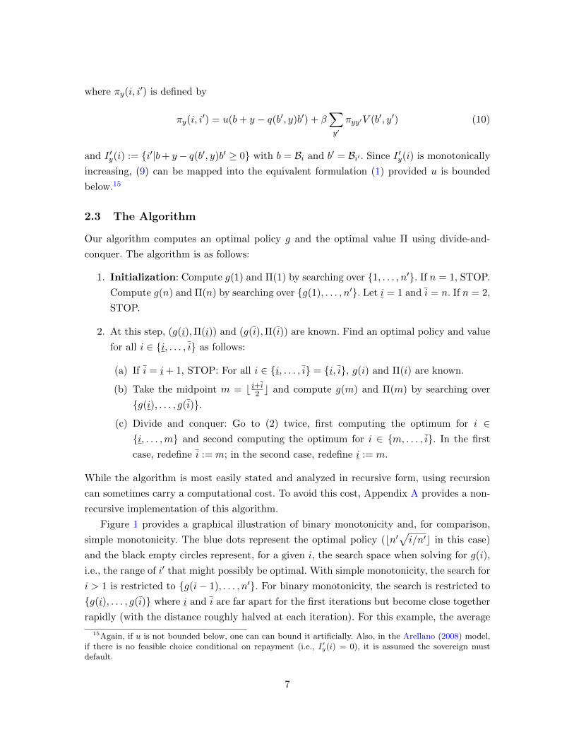
2.3 The Algorithm

Our algorithm computes an optimal policy g and the optimal value Π using divide-and-

conquer. The algorithm is as follows:

1. Initialization: Compute g(1) and Π(1) by searching over {1, . . . , n′}. If n = 1, STOP.

Compute g(n) and Π(n) by searching over {g(1), . . . , n′}. Let i = 1 and i = n. If n = 2,

STOP.

2. At this step, (g(i),Π(i)) and (g(i),Π(i)) are known. Find an optimal policy and value

for all i ∈ {i, . . . , i} as follows:

(a) If i = i+ 1, STOP: For all i ∈ {i, . . . , i} = {i, i}, g(i) and Π(i) are known.

(b) Take the midpoint m = b i+i2 c and compute g(m) and Π(m) by searching over

{g(i), . . . , g(i)}.

(c) Divide and conquer: Go to (2) twice, first computing the optimum for i ∈{i, . . . ,m} and second computing the optimum for i ∈ {m, . . . , i}. In the first

case, redefine i := m; in the second case, redefine i := m.

While the algorithm is most easily stated and analyzed in recursive form, using recursion

can sometimes carry a computational cost. To avoid this cost, Appendix A provides a non-

recursive implementation of this algorithm.

Figure 1 provides a graphical illustration of binary monotonicity and, for comparison,

simple monotonicity. The blue dots represent the optimal policy (bn′√i/n′c in this case)

and the black empty circles represent, for a given i, the search space when solving for g(i),

i.e., the range of i′ that might possibly be optimal. With simple monotonicity, the search for

i > 1 is restricted to {g(i− 1), . . . , n′}. For binary monotonicity, the search is restricted to

{g(i), . . . , g(i)} where i and i are far apart for the first iterations but become close together

rapidly (with the distance roughly halved at each iteration). For this example, the average

15Again, if u is not bounded below, one can can bound it artificially. Also, in the Arellano (2008) model,if there is no feasible choice conditional on repayment (i.e., I ′y(i) = 0), it is assumed the sovereign mustdefault.

7

search space for simple monotonicity, i.e. the average size of {g(i− 1), . . . , n′}, is 8.7 when

n = n′ = 20 and grows to 35.3 when n = n′ = 100. Since not exploiting monotonicity

would have the search space be 20 and 100, respectively, this represents roughly a 60%

improvement on brute force. In contrast, the average size of binary monotonicity’s search

space is 6.2 when n = n′ = 20 (a 29% improvement on simple monotonicity) and 8.9 when

n = n′ = 100 (a 75% improvement).

ii’

Binary monotonicity (n=n’=20)

i

i’

Simple monotonicity (n=n’=20)

Policy (g)

Search space

i

i’

Binary monotonicity (n=n’=100)

i

i’

Simple monotonicity (n=n’=100)

Figure 1: A Graphical Illustration of Simple and Binary Monotonicity

The remaining sections show that this example is typical. Specifically, in Section 3

we show that binary monotonicity always—i.e., for any monotone g—exhibits a very slow

increase in search space as n increases. In contrast, simple monotonicity may not exhibit

any reduction in search space (which is what happens when g(·) = 1). Then, in Section 4,

we show that, for both the RBC and Arellano (2008) models, simple monotonicity is about

60% faster than brute force but binary monotonicity is faster than simple monotonicity for

small grids and becomes increasingly faster as the grid size increases.

8

3 Theoretical Analysis

In the preceding algorithm, we assume there is some method for solving

maxi′∈{a,...,a+γ−1}

π(i, i′) (11)

for arbitrary a ≥ 1 and γ ≥ 1 (satisfying a + γ − 1 ≤ n′). One possibility is brute force

(checking every possible value), which requires γ evaluations of π(i, ·). However, if π(i, i′) is

known to be concave in i′, then Heer and Maußner (2005)’s binary concavity can find the

solution in no more than 2dlog2(γ)e − 1 for γ ≥ 3 and γ for γ ≤ 2.16 We allow for many

such methods by characterizing the algorithm’s properties conditional on a σ : Z++ → Z+,

restricting attention to monotonically increasing σ.

Because of the recursive nature of the algorithm, the π evaluation bound for general σ is

also naturally recursive. The following definition and Proposition 1 provide such a bound.

Definition. For any σ : Z++ → Z+, define Mσ : {2, 3, . . .} × Z+ → Z+ recursively by

Mσ(z, γ) = 0 if z = 2 or γ = 0 and

Mσ(z, γ) = σ(γ) + maxγ′∈{1,...,γ}

{Mσ(bz

2c+ 1, γ′) +Mσ(bz

2c+ 1, γ − γ′ + 1)

}for z > 2 and γ > 0.

Proposition 1. Let σ : Z++ → Z+ be an upper bound on the number of π evaluations

required to solve (11). Then, the algorithm requires at most 2σ(n′) +Mσ(n, n′) evaluations

where n and n′ are from the problem stated in (1) for n ≥ 2 and n′ ≥ 1.

While not as tight as possible, Proposition 1 gives a fairly tight bound. However, it is

also unwieldy because of the discrete nature of the problem. By bounding σ whose domain

is Z++ with a σ whose domain is [1,∞), a more convenient bound can be found. This bound

is given in Lemma 1.

Lemma 1. Suppose σ : [1,∞) → R+ is either the identity map (σ(γ) = γ) or is a strictly

increasing, strictly concave, and differentiable function. If σ(γ) ≥ σ(γ) for all γ ∈ Z++,

then an upper bound on function evaluations is

3σ(n′) +I−2∑j=1

2j σ(2−j(n′ − 1) + 1)

if I > 2 where I = dlog2(n− 1)e+ 1. An upper bound for I ≤ 2 is 3σ(n′).

16We prove this in Lemma 2 in Appendix B.

9

The main theoretical result of the paper is given in Proposition 2. It applies Lemma 1

with σ bounds corresponding to brute force concavity and binary concavity.

Proposition 2. Suppose n ≥ 4 and n′ ≥ 3. If brute force grid search is used, then no more

than log2(n− 1)(n′− 1) + 3n′+ 2n− 4 evaluations are required. Consequently, fixing n = n′

the algorithm’s worst case behavior is O(n log n) with a hidden constant of one.

If binary concavity is used, then no more than 10n+8n′−4 log2(n′−1)−32 evaluations

are required. Consequently, fixing n = n′ the algorithm’s worst case behavior is O(n) with a

hidden constant of 18.

These worst-case bounds show binary monotonicity is very powerful, even without an

assumption about concavity. The remainder of the paper assesses binary monotonicity’s

performance in two economic models commonly employed in practice. As will be seen,

binary monotonicity also does very well in the context of these models.

4 Comparison with Existing Grid Search Techniques

This section compares our method with existing grid search techniques, or what we now

call “speedups.” Table 1 lists all speedups known to us, along with brief descriptions of

each. We break the analysis into two parts. First, we compare our method with existing

speedups that do not assume concavity. For this, we use the Arellano (2008) model. Second,

we compare our method with existing speedups that do assume concavity. For this, we use

the RBC model since the Arellano (2008) model has non-concave value functions. Since

the accuracy of all the grid search methods is identical (because they all produce exactly

the same policy), we do not report any accuracy measures. Calibrations are presented in

Appendix C.

4.1 Not Assuming Concavity

Figure 2 reports the time required to obtain convergence in Arellano (2008) model for brute

force, simple monotonicity, and binary monotonicity (the only speedups that apply to this

non-concave problem). The run times for brute force and simple monotonicity both grow

exponentially. In contrast, binary monotonicity grows almost linearly. For a grid size of 100,

all the methods solve the model much less than a minute. This changes quickly with n. For

a 1000 point grid, brute force takes about 8 minutes, simple monotonicity takes about half

that, but binary monotonicity takes far less than a minute. In general, it seems that simple

monotonicity is about 50% faster than brute force.

Table 2, which gives run times and π evaluation counts for a wide range of n values,

confirms and extends these findings. Simple monotonicity requires roughly 60% fewer eval-

10

Grid Search Speedup Description

Simple Monotonicity Exploits policy function monotonicity by only searching i′ ∈{g(i− 1), . . . , n′} when i > 1.

Binary Monotonicity The approach in this paper. Uses divide-and-conquer to ex-ploit policy function monotonicity. Restricts search range toi′ ∈ {g(i), . . . , g(i)} .

Simple Concavity Exploits concavity of π(i, i′) in i′. To find the maximum ini′ ∈ {i, . . . , i}, iterates through i′ = i, i+1, . . . and stops onceπ(i, i′) decreases or i is reached.

Binary Concavity The approach in Heer and Maußner (2005). Uses divide-and-conquer to explot concavity of π(i, i′) in i′. In finding the

maximum of i′ ∈ {i, . . . , i}, checks i′ = b i+i2 c and i′ = b i+i2 c+1, then restricts search to only {i, b i+i2 c} or {b i+i2 c+ 1, i}.

X Monotonicity andY Concavity

UsesX monotonicity to restrict the search space for i′ to someinterval {i, . . . , i} and then Y concavity to find the maximumwithin that range.

Table 1: Description of Grid Search Speedups

100 500 1000 2500 5000 100000

5

10

15

20

25

30

Convergence Time (Minutes)

Grid Size (n)

Min

ute

s

Binary Monotonicity

Simple Monotonicity

Brute Force

Figure 2: Convergence Time For Methods Not Assuming Concavity

11

uations than brute force and so exhibits the same exponential growth in run times. The

running times and evaluation counts for binary monotonicity are less initially and grow

much more slowly in n. As a consequence, the ratio of the simple monotonicity running

time to the binary time begins at around 6 for a 100 point grid, grows to 50 for a 1000 point

grid, 400 for a 1000 point grid, and continues to grow close to linearly in n. Hence, even

for small grid sizes, one can expect a large speedup relative to simple monotonicity. Binary

monotonicity is so fast that it takes less than a minute for a 10,000 point grid and less

than ten minutes for a 100,000 point grid. In contrast, simple monotonicity’s run time for

a 10,000 point grid is 5 hours and (estimated) run time for a 100,000 point grid is roughly

three weeks.

Run Time (Minutes) Evaluations/n Simple toGrid size (n) None∗ Simple∗ Binary∗ None∗ Simple∗ Binary∗ Binary Time

100 0.08∗ 0.03∗ 0.01∗ 100∗ 42∗ 5.5∗ 6.1250 0.48∗ 0.20∗ 0.01∗ 250∗ 102∗ 6.1∗ 14.4500 1.90∗ 0.78∗ 0.03∗ 500∗ 204∗ 6.5∗ 26.71000 7.71∗ 3.16∗ 0.06∗ 1000∗ 406∗ 7.0∗ 51.42500 47.7∗ 19.3∗ 0.17∗ 2500∗ 1013∗ 7.6∗ 1165000 192∗ 78.6∗ 0.36∗ 5000∗ 2025∗ 8.0∗ 22010000 769∗ 309∗ 0.75∗ 10000∗ 4050∗ 8.5∗ 40925000 4814∗ 1914∗ 2.21∗ 25000∗ 10122∗ 9.1∗ 86750000 19264∗ 7634∗ 4.60∗ 50000∗ 20243∗ 9.5∗ 1659100000 77075∗ 30491∗ 8.91∗ 100000∗ 40484∗ 10.0∗ 3423

Note: ∗ means the value is estimated via a fitted quadratic polynomial.

Table 2: Run Times and Evaluations for Methods Not Assume Concavity

4.2 Assuming Concavity

The previous section showed that binary monotonicity outperforms existing grid search

methods that do not assume concavity. However, binary monotonicity can be combined

with various concavity speedups to deliver potentially much faster performance. Table 3

examines the running times for all nine combinations of the monotonicity and concavity

speedups. Since the Arellano (2008) model has non-concave value functions, the RBC model

is used.

Surprisingly, the fastest combination is simple monotonicity with simple concavity. This

pair has the smallest run times for both values of n and the time increases linearly. Somewhat

amazingly, to solve for the optimal policy for a given state requires, on average, only three

evaluations of π. The second fastest, binary monotonicity with binary concavity, exhibits

a similar linear time increase but fares slightly worse in absolute terms. In particular, it

12

Speedup n = 250 n = 500 TimeMonotonicity Concavity Eval./n Min. Eval./n Min. Increase

None None 250.0 1.15 500.0 4.59 4.0Simple None 127.0 0.40 252.5 1.58 4.0Binary None 10.7 0.06 11.7 0.14 2.2

None Simple 126.0 0.77 250.5 3.04 4.0Simple Simple 3.0 0.02 3.0 0.04 2.0Binary Simple 6.8 0.05 7.3 0.10 2.1

None Binary 13.9 0.09 15.9 0.20 2.3Simple Binary 12.6 0.07 14.6 0.16 2.3Binary Binary 3.7 0.03 3.7 0.05 2.0

Table 3: Run Times and Evaluations for All Monotonicity and Concavity Speedups

requires on average 3.7 evaluations of π per state, a very small number, but not quite

as small as the 3.0 required by simple concavity and simple monotonicity. All the other

combinations are slower and exhibit superlinear time increases.

Simple monotonicity paired with simple concavity is very effective because the policy

function is very nearly linear when the grid is uniform (as it is here). In particular, the capital

policy very nearly satisfies either g(i) = g(i−1) or g(i) = g(i−1)+1. In the first case, simple

monotonicity and simple concavity requires only two π evaluations to compute g(i) when

g(i−1) is known: The first evaluates π(i, g(i−1)) and the second evaluates π(i, g(i−1)+1);

finding π(i, g(i − 1)) ≥ π(i, g(i − 1) + 1), the algorithm terminates. In the second case, a

third evaluation, π(i, g(i−1)+2) is needed, but finding π(i, g(i−1)+1) ≥ π(i, g(i−1)+2),

the algorithm stops.

Whereas simple monotonicity with simple concavity searches locally about g(i − 1) in

computing g(i), the second fastest combination of binary monotonicity with binary concav-

ity performs something more akin to a global search. It finds g(i) not using information

about g(i − 1), but rather about g(a) and g(b) where i = b(a + b)/2c. The search space

is then restricted {g(a), . . . , g(b)}. If g(a + 1) = g(a) + 1 for all a, then the true solu-

tion is, loosely speaking, g(i) = g(a) + (a + b)/2. However, binary concavity search does

not use this information, but rather begins divide-and-conquer of the entire search domain

{g(a), . . . , g(b)}.17

17This suggests a heuristic of searching a small interval about g(a) + (a+ b)/2 first before expanding thesearch, if necessary, to all of {g(a), . . . , g(b)}. However, simple monotonicity with simple concavity wouldseemingly be preferable to this.

13

1000 10000 1000002

4

6

8

10

12

14

16

18

20

Average # of Evaluations Divided by n

Grid Size (n)

Evalu

ations

Simple Mono, Simple Conc

Binary Mono, No Conc

Binary Mono, Simple Conc

Binary Mono, Binary Conc

Figure 3: Empirical O(n) Behavior

5 Conclusion

We have shown binary monotonicity is a powerful grid search technique. Without any as-

sumptions of concavity, the algorithm is O(n log2 n) for any monotone policy. Discrete choice

models where monotonicity obtains but concavity does not should substantially benefit from

our approach. Our approach may enable Bayesian estimation of this class of models, em-

ploying the particle filter of Fernandez-Villaverde and Rubio-Ramırez (2007). When paired

with binary concavity, binary monotonicity is O(n) enabling grid search to be used for very

large problems.

References

S. R. Aiyagari. Uninsured idiosyncratic risk and aggregate savings. Quarterly Journal of

Economics, 109(3):659–684, 1994.

C. Arellano. Default risk and income fluctuations in emerging economies. American Eco-

nomic Review, 98(3):690–712, 2008.

C. D. Carroll. The method of endogenous gridpoints for solving dynamic stochastic opti-

mization problems. Economic Letters, 91(3):312–320, 2006.

14

S. Chatterjee, D. Corbae, M. Nakajima, and J.-V. Rıos-Rull. A quantitative theory of

unsecured consumer credit with risk of default. Econometrica, 75(6):1525–1589, 2007.

J. Fernandez-Villaverde and J. F. Rubio-Ramırez. Estimating macroeconomic models: A

likelihood approach. The Review of Economic Studies, 74(4):1059–1087, 2007.

B. Heer and A. Maußner. Dynamic General Equilibrium Modeling: Computational Methods

and Applications. Springer, Berlin, Germany, 2005.

P. Krusell and A. A. Smith, Jr. Income and wealth heterogeneity in the macroeconomy.

Journal of Political Economy, 106(5):867–896, 1998.

G. Tauchen. Finite state Markov-chain approximations to univariate and vector autoregres-

sions. Economics Letters, 20(2):177–181, 1986.

A Algorithms

This appendix contains a non-recursive version of binary monotonicity, as well as our im-

plementation of binary concavity.

A.1 A Non-Recursive Formulation of Binary Monotonicity

Rather than directly implementing binary monotonicity using recursion, it is computation-

ally more efficient to eliminate the recursion. The following algorithm does this:

1. Initialization: Compute g(1) maximizing over {1, . . . , n′} and compute g(n) maxi-

mizing over {g(1), . . . , n′}. Allocate an array of size (dlog2(n − 1)e + 1) × 2 that will

hold the list below. Fill the first row of the array with (l1, u1) where l1 := 1, u1 := n.

Define k := 1.

2. Expand the list from k rows to k rows as follows:

l1 u1...

...

lk uk

lk+1 uk+1

lk+2 uk+2

......

lk uk

:=

l1 u1...

...

lk uk

lk b lk+uk2 clk b lk+uk+1

2 c...

...

lk b lk+uk−1

2 c

15

stopping when uk ≤ lk + 1 (corresponding to step 2(a) in the algorithm). At this step,

k ≥ 1 and g(lj) and g(uj) are known for all j ≤ k. For j = k+1, . . . , k, compute g(uj)

by maximizing over the interval g(lj−1), . . . , g(uj−1). Taking each row as specifying

an interval and subdividing it into two intervals, the following row gives the leftmost

subinterval.

At this point, g is known for every l and u in the list. Moreover, the interval correspond-

ing to k has exactly two elements, lk and uk, which implies the policy g(lk), . . . , g(uk)

is known.

Define k := k. Go to step 3.

3. If k = 1, STOP. If uk = uk−1, then eliminate the last row of the list, set k := k − 1,

and repeat this step. Otherwise, go to the next step.

4. If here, then uk < uk−1. Set (lk, uk) := (uk, uk−1). This step corresponds to moving

to the right subinterval of the interval corresponding to k − 1. Go to step 2.

A.2 Binary Concavity

Below is our implementation of Heer and Maußner (2005)’s algorithm for solving

maxi′∈{a,...,b}

π(i, i′).

Throughout, n refers to b− a+ 1.

1. Initialization: If n = 1, compute the maximum, π(i, a), and STOP. Otherwise, set

the flags 1a = 0 and 1b = 0. These flags indicate whether the value of π(i, a) and

π(i, b) are known, respectively.

2. If n > 2, go to 3. Otherwise, n = 2. Compute π(i, a) if 1a = 0 and compute π(i, b) if

1b = 0. The optimum is the best of a, b.

3. If n > 3, go to 4. Otherwise, n = 3. If max{1a,1b} = 0, compute π(i, a) and set

1a = 1. Define m = a+b2 , and compute π(i,m).

(a) If 1a = 1, check whether π(i, a) > π(i,m). If so, the maximum is a. Otherwise,

the maximum is either m or b; redefine a = m, set 1a = 1, and go to 2.

(b) If 1b = 1, check whether π(i, b) > π(i,m). If so, the maximum is b. Otherwise,

the maximum is either a or m; redefine b = m, set 1b = 1, and go to 2.

16

4. Here, n ≥ 4. Define m = ba+b2 c and compute π(i,m) and π(i,m + 1). If π(i,m) <

π(i,m+ 1), a maximum is in {m+ 1, . . . , b}; redefine a = m+ 1, set 1a = 1, and go to

2. Otherwise, a maximum is in {a, . . . ,m}; redefine a = m, set 1b = 1, and go to 2.18

B Omitted Proofs and Lemmas

This section contains omitted proofs and lemmas. They are broken into two sections. Section

B.1 examines the properties of the binary monotonicity algorithm and to a lesser extent the

binary concavity algorithm. Section B.2 state in what sense (1) and (2) are equivalent and

proves their equivalence. As stated in the main text, σ is always assumed to be monotonically

increasing.

B.1 Algorithm properties

Lemma 2. Consider the problem maxi′∈{a,...,a+n−1} π(i, i′) for any a and any i. For any

n ∈ Z++, binary concavity requires no more 2dlog2(n)e − 1 evaluations if n ≥ 3 and no

more than n evaluations if n ≤ 2.

Proof. We will show σ(n) = 2dlog2(n)e − 1 for n ≥ 3 and σ(n) = n for n ≤ 2 is an upper

bound on the number of evaluations the binary concavity requires. For n = 1, the algorithm

computes π(i, a) and stops, so one evaluation is required. This agrees with σ(1) = 1. For

n = 2, two evaluations are required (π(i, a) and π(i, a + 1)). This agrees with σ(2) = 2.

For n = 3, step 3 requires π(i,m) to be computed and may require π(i, a) to be computed.

Then step 3(a) or step 3(b) either stop with no additional function evaluations or go to

step 2 with max{1a,1b} = 1 where, in that case, at most one additional function evaluation

is required. Consequently, n = 3 requires at most three function evaluations, which agrees

with σ(3) = 2dlog2(3)e − 1 = 3. So, the statement of lemma holds for 1 ≤ n ≤ 3.

Now consider each n ∈ {4, 5, 6, 7} for any 1a,1b flags. Since n ≥ 4 the algorithm is in

(or goes to) step 4. Consequently, two evaluations are required. Since the new interval is

either {a, . . . ,m} or {m+ 1, . . . , b} and π(i,m) and π(i,m+ 1) are computed in step 4, the

next step has max{1a,1b} = 1. Now, if n = 4, the next step must be step 2, which requires

at most one additional evaluation (since max{1a,1b} = 1). Hence, the total evaluations are

less than or equal to 3 (two for step 4 and one for step 2). If n = 5, then the next step is

either step 2, requiring one evaluation, or step 3, requiring two evaluations. So, the total

evaluations are not more than four. If n = 6, the next step is step 3, and so four evaluations

are required. Lastly, for n = 7, the next step is either step 3, requiring two evaluations, or

step 4 (with n = 4), requiring at most three evaluations. So, the evaluations are weakly less

18Note that in the case of indifference, π(i,m) = π(i,m+ 1), the algorithm proceeds to {a, . . . ,m}.

17

than 5 = 2 + max{2, 3}. Hence, for every n = 4, 5, 6, and 7, the required evaluations are

less than 3, 4, 4, and 5, respectively. One can then verify that the evaluations are less than

2dlog2(n)e − 1 for these values of n.

Now, suppose n ≥ 4. We shall prove that the required number of evaluations is less than

2dlog2(n)e − 1 (i.e., is less than σ(n)). The proof is by induction. We have already verified

the hypothesis holds for n ∈ {4, 5, 6, 7}, so consider some n ≥ 8 and suppose the hypothesis

holds for all m ∈ {4, . . . , n − 1}. Let i be such that n ∈ [2i + 1, 2i+1]. Then note that two

things are true, dlog2(n)e = i+1 and dlog2(bn+12 c)e = i.19 Since n ≥ 4, the algorithm is in (or

proceeds to) step 4, which requires two evaluations, and then proceeds with a new interval to

step 4 (again). If n is even, the new interval has size n/2. If n is odd, the new interval either

has a size of (n+1)/2 or (n−1)/2. So, if n is even, no more than 2+σ(n/2) evaluations are

required; if n is odd, no more than 2 + max{σ((n+ 1)/2), σ((n− 1)/2)} = 2 + σ((n+ 1)/2)

evaluations are required. The even and odd case can then be handled simultaneously with

the bound 2 + σ(bn+12 c). Manipulating this expression,

2 + σ(bn+ 1

2c) = 2 + 2dlog2b

n+ 1

2ce − 1

= 2 + 2i− 1

= 2(i+ 1)− 1

= 2dlog2(n)e − 1.

Hence, the proof by induction is complete.

Lemma 3. For any σ, Mσ(z, γ) is weakly increasing in z and γ.

Proof. Fix a σ and suppress dependence on it. First, we will show M(z, γ) is weakly in-

creasing in γ for every z. The proof is by induction. For z = 2, M(2, ·) = 0. For z = 3,

M(3, γ) = σ(γ) which is weakly increasing in γ. Now consider some z > 3 and suppose

M(y, ·) is weakly increasing for all y ≤ z − 1. For γ2 > γ1,

M(z, γ1) = σ(γ1) + maxγ′∈{1,...,γ1}

{M(bz

2c+ 1, γ′) +M(bz

2c+ 1, γ1 − γ′ + 1)

}≤ σ(γ2) + max

γ′∈{1,...,γ2}

{M(bz

2c+ 1, γ′) +M(bz

2c+ 1, γ1 − γ′ + 1)

}≤ σ(γ2) + max

γ′∈{1,...,γ2}

{M(bz

2c+ 1, γ′) +M(bz

2c+ 1, γ2 − γ′ + 1)

}= M(z, γ2)

19Note that both dlog2(·)e and dlog2(b·c)e are weakly increasing functions. So n ∈ [2i + 1, 2i+1] impliesdlog2(n)e ∈ [dlog2(2i + 1)e, dlog2(2i+1)e] = [i+ 1, i+ 1]. Likewise, n ∈ [2i + 1, 2i+1] implies dlog2(bn+1

2c)e ∈

[dlog2(b 2i+1+1

2c)e, dlog2(b 2

i+1+12c)e] = [i+ 1, i+ 1].

18

where the second inequality is justified by the induction hypothesis giving M(b z2c+ 1, ·) as

an increasing function (note b z2c+ 1 ≤ z − 1 for all z > 3).

Now we will show M(z, γ) is increasing in z for every γ. The proof is by induction.

First, note that M(2, γ) = 0 ≤ σ(γ) = M(3, γ) for all γ > 0 and M(2, γ) = 0 = M(3, γ)

for γ = 0. Now, consider some k > 3 and suppose that for any z1, z2 ≤ k − 1 with z1 ≤ z2

that M(z1, γ) ≤M(z2, γ) for all γ. The goal is to show that for any z1, z2 ≤ k with z1 ≤ z2that M(z1, γ) ≤M(z2, γ) for all γ. So, consider such z1, z2 ≤ k with z1 ≤ z2. If γ = 0, then

M(z1, γ) = 0 = M(z2, γ), so take γ > 0. Then

M(z1, γ) = σ(γ) + maxγ′∈{1,...,γ}

{M(bz1

2c+ 1, γ′) +M(bz1

2c+ 1, γ − γ′ + 1)

}≤ σ(γ) + max

γ′∈{1,...,γ}

{M(bz2

2c+ 1, γ′) +M(bz2

2c+ 1, γ − γ′ + 1)

}= M(z2, γ).

The inequality obtains since b zi2 c + 1 ≤ k − 1 for all i (which is true since even if zi = k,

one has bk/2c + 1 ≤ k − 1 by virtue of k > 3) and so the induction hypothesis gives

M(b z12 c+ 1, ·) ≤M(b z22 c+ 1, ·). Hence, the proof by induction is complete.

Proof of Proposition 1.

Proof. Since g is the policy function associated with (1), g : {1, . . . , n} → {1, . . . , n′}. By

monotonicity, g is weakly increasing. Define N : {1, . . . , n}2 → Z+ by

N(a, b) = M(b− a+ 1, g(b)− g(a) + 1)

noting that this is well-defined (based on the definition of M) whenever b > a. Additionally,

define a sequence of sets Ik for k = 1, . . . , n− 1 by

Ik := {(i, i)|i = i+ k and i, i ∈ {1, . . . , n}}.

Note that for any k ∈ {1, . . . , n − 1}, Ik is nonempty and N(a, b) is well-defined for any

(a, b) ∈ Ik.We shall now prove that for any k ∈ {1, . . . , n−1}, (i, i) ∈ Ik implies N(i, i) is an upper

bound on the number of evaluations of π required by the algorithm in order to compute the

optimal policy for all i ∈ {i, . . . , i} when g(i) and g(i) are known. If true, then beginning

at step 2 in the algorithm (which assumes g(i) and g(i) are known) with (i, i) ∈ Ik, N(i, i)

is an upper bound on the number of π evaluations.

The argument is by induction. First, consider k = 1. For any (a, b) ∈ I1, the algorithm

19

terminates at step 2(a). Consequently, the number of required π evaluations is zero, which

is the same as N(a, b) = M(b − a + 1, g(b) − g(a) + 1) = M(2, g(b) − g(a) + 1) = 0 (recall

M(2, ·) = 0).

Now, consider some k ∈ {2, . . . , n − 1} and suppose the induction hypothesis holds for

all j in 1, . . . , k − 1. That is, assume for all j in 1, . . . , k − 1 that (i, i) ∈ Ij implies N(i, i)

is an upper bound on the number of required π evaluations when g(i) and g(i) are known.

We shall show it holds for k as well.

Consider any (i, i) ∈ Ik with g(i) and g(i) are known. Since i > i+1, the algorithm does

not terminate at step 2(a). In step 2(b), to compute g(m) (where m := b i+i2 c), one must

find the maximum within the range g(i), . . . , g(i), which requires at most σ(g(i)− g(i) + 1)

evaluations of π. In step 2(c), the space is then divided into {i, . . . ,m} and {m, . . . , i}.If k is even, then m equals i+i

2 . Since (i,m) ∈ Ik/2 and g(i) and g(m) are known,

the induction hypothesis gives N(i,m) as an upper bound on the number of π evaluations

needed to compute g(i), . . . , g(m). Similarly, since (m, i) ∈ Ik/2 and g(m) and g(i) are

known, N(m, i) provides an upper bound on the number of π evaluations needed to compute

g(m), . . . , g(i). Therefore, to compute g(i), . . . , g(i), at most σ(g(i)− g(i) + 1) +N(i,m) +

N(m, i) evaluations are required. Defining γ = g(i)− g(i) + 1 and γ′ = g(m)− g(i) + 1 and

using the definition of m and N , we have that the number of required evaluations is less

than

σ(γ) +M(m− i+ 1, g(m)− g(i) + 1) +M(i−m+ 1, g(i)− g(m) + 1)

= σ(γ) +M(i+ i

2− i+ 1, γ′) +M(i− i+ i

2+ 1, g(i)− g(m) + 1)

= σ(γ) +M(i− i

2+ 1, γ′) +M(

i− i2

+ 1, g(i)− g(m) + γ′ − γ′ + 1)

= σ(γ) +M(i− i

2+ 1, γ′) +M(

i− i2

+ 1, g(i)− g(m) + g(m)− g(i) + 1− γ′ + 1)

= σ(γ) +M(i− i

2+ 1, γ′) +M(

i− i2

+ 1, γ − γ′ + 1).

By virtue of montonicity, g(m) ∈ {g(i), . . . , g(i)} and so g(m) − g(i) + 1 ∈ {1, . . . , g(i) −g(i) + 1} or equivalently γ′ ∈ {1, . . . , γ}. Consequently, the number of function evaluations

is not greater than

σ(γ) + maxγ′∈{1,...,γ}

{M

(i− i

2+ 1, γ′

)+M

(i− i

2+ 1, γ − γ′ + 1

)}.

The case of k odd is very similar, but the divide-and-conquer algorithm splits the space

unequally. If k is odd, then m equals i+i−12 . In this case (i,m) ∈ I(k−1)/2 and (m, i) ∈

20

I(k−1)/2+1.20 Consequently, computing the policy for i, . . . , i takes no more than σ(g(i) −

g(i)− 1) +N(i,m) +N(m, i) maximization steps. Defining γ and γ′ the same as before and

using the definition of m and N , we have the the required maximization steps is less than

σ(γ) +M(m− i+ 1, γ′) +M(i−m+ 1, γ − γ′ + 1)

= σ(γ) +M(i+ i− 1

2− i+ 1, γ′) +M(i− i+ i− 1

2+ 1, γ − γ′ + 1)

= σ(γ) +M

(i− i+ 1

2, γ′)

+M

(i− i+ 1

2+ 1, γ − γ′ + 1

)where γ and γ′ are defined the same as before. Because M is increasing in the first argument,

this is less than

σ(γ) + maxγ′∈{1,...,γ}

{M(

i− i+ 1

2+ 1, γ′) +M(

i− i+ 1

2+ 1, γ − γ′ + 1)

}.

Combining the bounds for k even and odd, the required number of π evaluations is less

than

σ(γ) + maxγ′∈{1,...,γ}

{M(b i− i+ 1

2c+ 1, γ′) +M(b i− i+ 1

2c+ 1, γ − γ′ + 1)

}(*)

because if k is even, then b i−i+12 c = i−i

2 . Consequently, (*) gives an upper bound for any

(i, i) ∈ Ik for k ≥ 1 when g(i) and g(i) are known. If N(i, i) is less than this, then the proof

by induction is complete.

Since N(i, i) is defined as M(i− i+ 1, g(i)− g(i) + 1), using the definitions of N and M

shows

N(i, i) = M(i− i+ 1, g(i)− g(i) + 1)

= M(i− i+ 1, γ)

= σ(γ) + maxγ′∈{1,...,γ}

{M(b i− i+ 1

2c+ 1, γ′) +M(b i− i+ 1

2c+ 1, γ − γ′ + 1)

}.

Consequently, N(i, i) exactly equals the value in (*), and the proof by induction is complete.

Step 1 of the algorithm requires at most 2σ(n′) evaluations to compute g(1) and g(n).

If n = 2, step 2 is never reached. Since M(n, n′) = 0 in this case, 2σ(n′) +M(n, n′) provides

an upper bound. If n > 2, then since (1, n) ∈ In−1 and g(1) and g(n) known, only N(1, n)

additional evaluations are required. Therefore, to compute for each i ∈ {1, . . . , n}, no more

20To see this, note that (i, i) ∈ Ik implies k = i−i. To have, (i,m) ∈ I(k−1)/2, it must be that m = i+ k−12

.

This holds: i+ k−12

= i+ i−i−12

= i+ i+i−1−i−i2

= i+m+ −2i2

= m. Similarly, to have (m, i) ∈ I(k−1)/2+1,

one must have i = m+ (k− 1)/2 + 1. This also obtains: m+ (k−1)2

+ 1 = i+i−12

+ i−i−12

+ 1 = 2i−22

+ 1 = i.

21

than 2σ(n′) + N(1, n) = 2σ(n′) + M(n, g(n) − g(1) + 1) function evaluations are needed.

Lemma 3) then gives that this is less than 2σ(n′)+M(n, n′) since g(n)−g(1)+1 ≤ n′−1+1 =

n′.

Lemma 4. Define a sequence {mi}∞i=1 by m1 = 2 and mi = 2mi−1 − 1 for i ≥ 2. Then

mi = 2i−1 + 1 and log2(mi − 1) = i− 1 for all i ≥ 1.

Proof. The proof of mi = 2i−1 + 1 for all i ≥ 1 is by induction. For i = 1, m1 is defined as

2, which equals 21−1 + 1. For i > 1, suppose it holds for i− 1. Then

mi = 2mi−1 − 1

= 2[2i−2 + 1]− 1

= 2i−1 + 1.

Lemma 5. Consider any z ≥ 2. Then there exists a unique sequence {ni}Ii=1 such that

n1 = 2, nI = z, bni2 c+ 1 = ni−1, and ni > 2 for all i > 1. Moreover, I = dlog2(z − 1)e+ 1.

Proof. The proof that a unique sequence exists is by construction. Let z ≥ 2 be fixed.

Define an infinite sequence {zi}∞i=1 recursively as follows: Define zi = Ti(z) for all i ≥ 1

with T1(z) := z and Ti+1(z) = bTi(z)2 c+ 1. We now establish all of the following: Ti(z) ≥ 2,

Ti(z) ≥ Ti+1(z), and Ti(z) > Ti+1(z) whenever Ti(z) > 2. As an immediate consequence,

for any z ≥ 2, there exists a unique I(z) ≥ 1 such that TI(z) = 2 and, for all i < I(z),

Ti(z) > 2. We also show for later use that Ti(z) is weakling increasing in z for every i.

To show Ti(z) ≥ 2, the proof is by induction. We have T1(z) = z and z ≥ 2. Now,

consider some i > 1 and suppose it holds for i−1. Then Ti(z) = bTi−1(z)2 c+1 ≥ b22c+1 = 2.

To show Ti(z) > Ti+1(z) whenever Ti(z) > 2, consider two cases. First, consider Ti(z)

even. Then Ti+1(z) = bTi(z)2 c + 1 = Ti(z)2 + 1 and so Ti+1(z) < Ti(z) as long as Ti(z) > 2.

Second, consider Ti(z) odd. Then Ti+1(z) = bTi(z)2 c+ 1 = Ti(z)−12 + 1 and so Ti+1(z) < Ti(z)

as long as Ti(z) > 1.

To show that Ti(z) ≥ Ti+1(z), all we need to show now is that Ti+1(z) = 2 when

Ti(z) = 2 (since the inequality is strict if Ti(z) > 2 and Ti(z) ≥ 2 for all i). If Ti(z) = 2,

then Ti+1(z) = b22c+ 1 = 2.

To establish that Ti(z) is weakly increasing in z for every i, the proof is by induction.

For a ≤ b, T1(a) = a ≤ b = T1(b). Now consider some i > 1 and suppose the induction

hypothesis holds for i− 1. Then Ti(a) = bTi−1(a)/2c+ 1 ≤ bTi−1(b)/2c+ 1 = Ti(b).

22

The sequence {nj}I(z)j=1 defined by nj = TI(z)−j+1(z)—i.e., an inverted version of the

sequence {Ti(z)}I(z)i=1—satisfies nI(z) = T1(z) = z, n1(z) = TI(z) = 2, and ni−1 =

TI(z)−(i−1)+1 = bTI(z)−(i−1)

2 c + 1 = bni2 c + 1. Also, by the definition of I(z), Ti(z) > 2

for any i > I(z). So, if we can show that I(z) = dlog2(z − 1)e+ 1, the proof is complete.

The proof of I(z) = dlog2(z − 1)e + 1 is as follows. Note that for z = 2, the sequence

{zi} is simply zi = 2 for all i which implies I(2) = 1. Since dlog2(2 − 1)e + 1 = 1, the

relationship holds for z = 2. So, now consider z > 2. The proof proceeds in the following

steps. First, for the special {mi} sequence defined in Lemma 4, we show Tj(mi) = mi+1−j

for any i ≥ 1 and any j ≤ i. Second, we use this to show that I(mi) = i for all i ≥ 1. Third,

we show that z ∈ (mi−1,mi] implies I(z) = i by showing I(mi−1) < I(z) ≤ I(mi). Fourth,

we show that the i such that z ∈ (mi−1,mi] is given by dlog2(z − 1)e + 1. This then gives

I(z) = dlog2(z − 1)e+ 1 since I(z) = I(mi) = i = dlog2(z − 1)e+ 1.

First, we show Tj(mi) = mi+1−j for any i ≥ 1 and any j ≤ i. Fix some i ≥ 1. The proof

is by induction. For j = 1, T1(mi) = mi = mi+1−1. Now consider some j having 2 ≤ j ≤ i

and suppose the induction hypothesis holds for j − 1. Then

Tj(mi) = bTj−1(mi)

2c+ 1

= bmi+1−(j−1)

2c+ 1

= bmi+2−j2c+ 1

= b2mi+1−j − 1

2c+ 1

= mi+1−j + b−1

2c+ 1

= mi+1−j − 1 + 1

= mi+1−j ,

which proves Tj(mi) = mi+1−j for j ≤ i.Second, we show I(mi) = i for all i ≥ 1. Consider any i ≥ 1. Then Tj(mi) = mi+1−j

for all j ≤ i. Note then that m1 = 2 and mj ≥ 3 for all j ≥ 2. Since I(z) is defined as the

unique value such that TI(z)(z) = 2 and j < I(z) implies Tj(z) > 2, we must have I(mi) = i

because Ti(mi) = 2 and j < i implies Tj(mi) = mi+1−j ≥ mi+1−(i−1) = m2 > 2.

Third, we show that z ∈ (mi−1,mi] implies I(z) by showing I(mi − 1) < I(z) ≤ I(mi).

Note that, since z > 2 (having taken care of the z = 2 case already), there is some i ≥ 2 such

that z ∈ (mi−1,mi] (since m1 = 2). To see I(z) ≤ I(mi), suppose not, that I(z) > I(mi).

But then 2 = TI(z)(z) < TI(mi)(z) ≤ TI(mi)(mi) = 2, which is a contradiction.21 Therefore,

21The second inequality uses that Ti(z) is weakly increasing in z for every i, as established above.

23

I(z) ≤ I(mi).

To see I(mi−1) < I(z), we begin by showing Tj(mi−1) < Tj(mi−1 + ε) for any ε > 0 and

any j ≤ i − 1. It is equivalent to show mi−j < Tj(mi−1 + ε), which we show by induction.

Clearly, for j = 1, we have mi−1 < mi−1 + ε = T1(mi−1 + ε). Now consider j > 1 and

suppose it is true for j − 1. Then

Tj(mi−1 + ε) = bTj−1(mi−1 + ε)

2c+ 1

= bTj−1(mi−1 + ε)−mi−j+1 +mi−j+1

2c+ 1

= bTj−1(mi−1 + ε)−mi−j+1 + 2mi−j − 1

2c+ 1

= bTj−1(mi−1 + ε)−mi−j+1 − 1

2c+mi−j + 1

Now, since the induction hypothesis of Tj−1(mi−1 + ε) > mi−j+1 gives Tj−1(mi−1 + ε) −mi−j+1 − 1 ≥ 0, one has

Tj(mi−1 + ε) ≥ b02c+mi−j + 1

= mi−j + 1

> mi−j .

Hence the proof by induction is complete.

Now, having established Tj(mi−1) < Tj(mi−1 + ε) for any ε > 0 and any j ≤ i − 1,

we show I(mi−1) < I(z). Suppose not, that I(mi−1) ≥ I(z). Then since z > mi−1, taking

ε = z−mi−1 we have 2 = TI(mi−1)(mi−1) < TI(mi−1)(mi−1+ε) = TI(mi−1)(z) ≤ TI(z)(z) = 2,

which is a contradiction.

Lastly, we now show that the i such that z ∈ (mi−1,mi] is given by dlog2(z − 1)e + 1.

That this holds can be seen as follows. Note that z ∈ (mi−1,mi] implies log2(z − 1) + 1 ∈(log2(mi−1− 1) + 1, log2(mi− 1) + 1]. Then, since log2(mj − 1) + 1 = j (from Lemma 4), we

have log2(z− 1) + 1 ∈ (i− 1, i]. Then, by the definition of d·e, one has dlog2(z− 1) + 1e = i,

which of course is equivalent to dlog2(z − 1)e+ 1 = i. So, I(z) = dlog2(z − 1)e+ 1.

Proof of Lemma 1.

Proof. Fix some z ≥ 2 (the z corresponds to n above, and we will characterize the upper

bound for arbitrary, but fixed, z and any γ, which corresponds to n′). By Lemma 5, there

is a strictly monotone increasing sequence {zi}Ii=1 with zI = z, zi = b zi+1

2 c + 1 for i < I,

and with I = dlog2(z − 1)e+ 1 (and having z1 = 2).

24

For i > 1, define

W (zi, γ) := maxγ′∈{1,...,γ}

M(zi−1, γ′) +M(zi−1, γ − γ′ + 1)

and for i = 1 define W (zi, γ) = 0. The definition of M gives M(zi, γ) = σ(γ) +W (zi, γ) for

any i > 1 with M(z1, ·) = 0. Note that W (z2, γ) = W (z1, γ) = 0.

Define W—an upper bound and continuous version of W—as

W (zi, γ) := σ∗(γ) + maxγ′∈[1,γ]

W (zi−1, γ′) + W (zi−1, γ − γ′ + 1)

for i > 2 with σ∗(γ) defined as maxγ′∈[1,γ] σ(γ′) + σ(γ − γ′ + 1). For i = 1 or 2, define

W (zi, γ) = 0. Then W (zi, γ) ≤ W (zi, γ) for all i ≥ 1 and all γ ∈ Z++. The proof is by

induction. They are equal for i = 1 and i = 2. Now consider an i > 2 and suppose it holds

for i− 1.

W (zi, γ) = maxγ′∈{1,...,γ}

σ(γ′) + σ(γ − γ′ + 1) +W (zi−1, γ′) +W (zi−1, γ − γ′ + 1)

≤ maxγ′∈{1,...,γ}

σ(γ′) + σ(γ − γ′ + 1) + maxγ′∈{1,...,γ}

W (zi−1, γ′) +W (zi−1, γ − γ′ + 1)

≤ maxγ′∈{1,...,γ}

σ(γ′) + σ(γ − γ′ + 1) + maxγ′∈{1,...,γ}

W (zi−1, γ′) + W (zi−1, γ − γ′ + 1)

≤ maxγ′∈[1,γ]

σ(γ′) + σ(γ − γ′ + 1) + maxγ′∈[1,γ]

W (zi−1, γ′) + W (zi−1, γ − γ′ + 1)

≤ σ∗(γ) + maxγ′∈[1,γ]

W (zi−1, γ′) + W (zi−1, γ − γ′ + 1)

= W (zi, γ)

If σ(γ) = γ, then σ(γ′)+σ(γ−γ′+1) = γ+1 which does not depend on γ′. So, σ∗(γ) = γ+

1 = 2σ(γ+12 ). If the σ function is strictly increasing, strictly concave, and differentiable, then

the first order condition of the σ∗(γ) problem yields σ′(γ′) = σ′(γ − γ′ + 1). The derivative

is invertible (by strict concavity) and so γ′ = γ+12 . So, σ∗(γ) = σ(γ+1

2 ) + σ(γ − γ+12 + 1),

which gives σ∗(γ) = 2σ(γ+12 ), the same condition as in the linear case.22 So, for i > 2,

W (zi, γ) = 2σ(γ + 1

2) + max

γ′∈[1,γ]W (zi−1, γ

′) + W (zi−1, γ − γ′ + 1).

We will now show for i > 2 that W (zi, γ) = 2σ(γ+12 ) + 2W (zi−1,

γ+12 ), which gives a

simple recursive relationship for the upper bound (for i = 1 or 2, W (zi, γ) = 0). To do this,

22Since this is an interior solution and the problem is concave, the constraint γ′ ∈ [1, γ] is not binding.

25

we will prove by induction that for any i ≥ 2 and any γ that

maxγ′∈[1,γ]

W (zi, γ′) + W (zi, γ − γ′ + 1) = 2W (zi,

γ + 1

2),

which, as a consequence, immediately gives for i > 2 that

W (zi, γ) = 2σ(γ + 1

2) + max

γ′∈[1,γ]W (zi−1, γ

′) + W (zi−1, γ − γ′ + 1)

= 2σ(γ + 1

2) + 2W (zi−1,

γ + 1

2).

For i = 2, the induction hypothesis clearly holds. So consider some i > 2 and suppose it

holds for i− 1. Now,

maxγ′∈[1,γ]

W (zi, γ′) + W (zi, γ − γ′ + 1)

= maxγ′∈[1,γ]

2σ(γ′ + 1

2) + 2W (zi−1,

γ′ + 1

2) + 2σ(

(γ − γ′ + 1) + 1

2) + 2W (zi−1,

(γ − γ′ + 1) + 1

2)

= 2 maxγ′∈[1,γ]

σ(γ′ + 1

2) + σ(

γ + 1

2− γ′ + 1

2+ 1) + W (zi−1,

γ′ + 1

2) + W (zi−1,

γ + 1

2− γ′ + 1

2+ 1)

= 2 maxγ′∈[1, γ+1

2]σ(γ′) + σ(

γ + 1

2− γ′ + 1) + W (zi−1, γ

′) + W (zi−1,γ + 1

2− γ′ + 1)

≤ 2 maxγ′∈[1, γ+1

2]σ(γ′) + σ(

γ + 1

2− γ′ + 1) + 2 max

γ′∈[1, γ+12

]W (zi−1, γ

′) + W (zi−1,γ + 1

2− γ′ + 1)

= 2σ∗(γ + 1

2) + 2 · 2W (zi−1,

γ+12 + 1

2)

= 2 · 2σ(γ+12 + 1

2) + 2 · 2W (zi−1,

γ+12 + 1

2)

= 2

(2σ(

γ+12 + 1

2) + 2W (zi−1,

γ+12 + 1

2)

)= 2W (zi,

γ + 1

2)

This establishes maxγ′∈[1,γ] W (zi, γ′)+W (zi, γ−γ′+1) ≤ 2W (zi,

γ+12 ). However, 2W (zi,

γ+12 )

is just W (zi, γ′)+W (zi, γ−γ′+1) evaluated at γ+1

2 , and so maxγ′∈[1,γ] W (zi, γ′)+W (zi, γ−

γ′ + 1) ≥ 2W (zi,γ+12 ). Hence, they are equal, and the proof by induction is complete.

Now, fix any γ ≥ 1 (corresponding to n′ in the statement of the lemma) and define

26

γI := γ and γi = γi+1+12 . Then γi = 2i−I(γI − 1) + 1.23 Then, for i > 2,

W (zi, γi) = 2σ(γi−1) + 2W (zi−1, γi−1).

So, if I > 2, repeatedly expand the expression to find a value for W (zI , γI):

W (zI , γI) = 2σ(γI−1) + 2W (zI−1, γI−1)

= 2σ(γI−1) + 22σ(γI−2) + 22W (zI−2, γI−2)

= 2σ(γI−1) + . . .+ 2I−2σ(γ2) + 2I−2W (z2, γ2)

= 2σ(γI−1) + . . .+ 2I−2σ(γ2)

=I−2∑j=1

2j σ(γI−j)

=

I−2∑j=1

2j σ(2I−j−I(γI − 1) + 1)

=I−2∑j=1

2j σ(2−j(γI − 1) + 1)

If I ≤ 2, then W (zI , γI) = 0.

Proposition 1 shows the number of required evaluations is less than or equal to 2σ(γI)+

M(zI , γI) for zI ≥ 2 and γI ≥ 1. Since M(zi, γ) = σ(γ) + W (zi, γ) for any i > 1 (with

M(z1, γ) = 0) and W (zi, γ) ≤ W (zi, γ), the required function evaluations are weakly less

than 3σ(γI) + W (zI , γI) for any I (recalling W (zI , γI) = 0 for I ≤ 2). Hence, if I > 2, then

an upper bound is

3σ(γI) +

I−2∑j=1

2j σ(2−j(γI − 1) + 1)

and if I ≤ 2 an upper bound is 3σ(γI).

Proof of Proposition 2.

Proof. Define W (n, n′) =∑I−2

j=1 2j(2−j(n′−1)+1) where I = dlog2(n−1)e+1. Since n ≥ 4,

23The proof of this is by induction. First note for i = I since γI+12

= 2(I−1)−I(γI−1)+1. Now if let inductive

hypothesis be γj+1 = 2j+1−I(γI − 1) + 1, then it follows immediately that γj =γj+1+1

2= 2j+1−I (γI−1)+2

2.

And the induction is completed.

27

I > 2. In the case of brute force with σ(γ) = γ,

W (n, n′) = (I − 2)(n′ − 1) +I−2∑j=1

2j

= (I − 2)(n′ − 1) + 2I−1 − 2

= (I − 2)(n′ − 1) + 2dlog2(n−1)e − 2

≤ (I − 2)(n′ − 1) + 2log2(n−1)+1 − 2

≤ (I − 2)(n′ − 1) + 2(n− 1)− 2

≤ (I − 2)(n′ − 1) + 2n− 4

≤ (dlog2(n− 1)e − 1)(n′ − 1) + 2n− 4

≤ log2(n− 1)(n′ − 1) + 2n− 4

So, no more than log2(n− 1)(n′ − 1) + 3n′ + 2n− 4 evaluations are required.

In the case of binary concavity, Lemma 2 shows σ(γ) = 2dlog2(γ)e − 1 for γ ≥ 3 and

σ(γ) = γ for γ ≤ 3 is an upperbound. Now consider σ(γ) = 2 log2(γ) + 1. It is a strictly

increasing, strictly concave, and differentiable function. For γ = 1 or 2, one can plug in values

to find σ(γ) ≤ σ(γ). Additionally, for γ ≥ 3, σ(γ) ≤ 2dlog2(γ)e−1 ≤ 2(1+log2(γ))−1 = σ(γ)

So, it satisfies σ satisfies all the conditions of Lemma 1.

Plugging in, one finds

W (n, n′) =

I−2∑j=1

2j[1 + 2 log2(2

−j(n′ − 1) + 1)]

= (2I−1 − 2) + 2I−2∑j=1

2j log2(2−j(n′ − 1) + 1)

To handle the log2(2−j(n′− 1) + 1) term, we break the summation into two parts, one with

2−j(n′ − 1) < 1 and one with 2−j(n′ − 1) ≥ 1. We do this to exploit the following fact: For

x ≥ 1, log2(x+1) ≤ log2(x)+1 since they are equal at x = 1 the right hand side grows more

28

quickly in x (i.e., the derivative of log2(x+ 1) is less than the derivative of log2(x) + 1).

W (n, n′) = (2I−1 − 2) + 2I−2∑j=1

1[2−j(n′ − 1) < 1]2j log2(2−j(n′ − 1) + 1)

+ 2

I−2∑j=1

1[2−j(n′ − 1) ≥ 1]2j log2(2−j(n′ − 1) + 1)

≤ (2I−1 − 2) + 2I−2∑j=1

1[2−j(n′ − 1) < 1]2j

+ 2I−2∑j=1

1[2−j(n′ − 1) ≥ 1]2j log2(2−j(n′ − 1) + 1)

≤ (2I−1 − 2) + 2

I−2∑j=1

2j + 2

I−2∑j=1

1[2−j(n′ − 1) ≥ 1]2j log2(2−j(n′ − 1) + 1)

= 3(2I−1 − 2) + 2I−2∑j=1

1[2−j(n′ − 1) ≥ 1]2j log2(2−j(n′ − 1) + 1)

Now, exploiting log2(x+ 1) ≤ log2(x) + 1 for x ≥ 1,

≤ 3(2I−1 − 2) + 2I−2∑j=1

1[2−j(n′ − 1) ≥ 1]2j [1 + log2(2−j(n′ − 1))]

≤ 5(2I−1 − 2) + 2

I−2∑j=1

1[2−j(n′ − 1) ≥ 1]2j log2(2−j(n′ − 1))

= 5(2I−1 − 2) + 2I−2∑j=1

1[j ≤ log2(n′ − 1)]2j log2(2

−j(n′ − 1))

= 5(2I−1 − 2) + 2

dlog2(n′−1)e∑j=1

2j log2(2−j(n′ − 1))

= 5(2I−1 − 2) + 2

dlog2(n′−1)e∑j=1

2j(log2(n′ − 1)− j)

= 5(2I−1 − 2) + 2 log2(n′ − 1)

dlog2(n′−1)e∑j=1

2j − 2

dlog2(n′−1)e∑j=1

2jj

Then defining J = dlog2(n′ − 1)e and using that (for r 6= 1)

∑bj=a jr

j = ara−brb+1

1−r +

29

ra+1−rb+1

(1−r)2 ,24

W (n, n′) ≤ 5(2I−1 − 2) + 2 log2(n′ − 1)[2J+1 − 2]− 2

[−2 + J2J+1 + 22 − 2J+1

]= 5(2I−1 − 2) + log2(n

′ − 1)[2J+2 − 4]− 4− (J − 1)2J+2

= 5 · 2I−1 + log2(n′ − 1)[2J+2 − 4]− (J − 1)2J+2 − 14

= 5 · 2I−1 + log2(n′ − 1)[2dlog2(n

′−1)e+2 − 4]− (J − 1)2dlog2(n′−1)e+2 − 14

≤ 5 · 2I−1 + log2(n′ − 1)[(n′ − 1)23 − 4]− (J − 1)(n′ − 1)23 − 14

= 5 · 2I−1 + log2(n′ − 1)[8(n′ − 1)− 4]− (dlog2(n

′ − 1)e − 1)8(n′ − 1)− 14

≤ 5 · 2I−1 + log2(n′ − 1)[8(n′ − 1)− 4]− (log2(n

′ − 1)− 1)8(n′ − 1)− 14

= 5 · 2dlog2(n−1)e − 4 log2(n′ − 1) + 8(n′ − 1)− 14

≤ 10(n− 1)− 4 log2(n′ − 1) + 8n′ − 22

= 10n+ 8n′ − 4 log2(n′ − 1)− 32

B.2 Equivalence between the two problems

This subsection establishes the equivalence between (1) and (2). Currently, the notation for

the π and π problems are the opposite of what is in the main text.

Suppose I ′(i) ⊂ {1, . . . , n′} may be empty, but is monotonically increasing. Let I =

{i|i ∈ {1, . . . , n}, I ′(i) 6= ∅} so that i ∈ I has a feasible solution. For all i ∈ I, let

Π(i) := maxi′∈I′(i)

π(i, i′).

and let G(i) := arg maxi′∈I′(i) π(i, i′). Let G be the set of optimal policies, i.e., for every

g ∈ G and every i ∈ I, g(i) ∈ G(i). Further, suppose there is a π such that π(i, i′) > π for

all i ∈ I and i′ ∈ I ′(i) (i.e., π is bounded below, strictly, whenever defined).

Define

Π(i) = maxi′∈{1,...,n′}

π(i, i′)

and

π(i, i′) =

π(i, i′) if I ′(i) 6= ∅ and i′ ∈ I ′(i)π if I ′(i) 6= ∅ and i′ /∈ I ′(i)1[i′ = 1] if I ′(i) = ∅

24To find the value of the weighted geometric series, define S =∑bj=a jr

j , cancel terms to find (1− r)S =

ara−brb+1 + ra+1−rb+1

1−r , apply the usual formula for the (non-weighted) geometric series, and divide throughby 1− r.

30

Similarly, let G(i) := arg maxi′∈{1,...,n′} π(i, i′). Let G be the set of optimal policies, i.e., for

every g ∈ G and every i ∈ {1, . . . , n}, g(i) ∈ G(i).

Lemma 6. All of the following are true:

1. Π(i) = Π(i) for all i ∈ I.

2. G(i) = G(i) for all i ∈ I.

3. If every g ∈ G is weakly increasing, then every g ∈ G is also weakly increasing. NOTE:

This requires I ′(i) to be monotonically increasing, as is assumed, so that the infeasible

region is {1, . . . , i− 1} and G(i) in the infeasible region equals {1}.

Proof. For the proof of the first claim, let i ∈ I. Then I ′(i) 6= ∅. Therefore,

Π(i) = maxi′∈{1,...,n′}

π(i, i′) = max{π, maxi′∈I′(i)

π(i, i′)} = maxi′∈I′(i)

π(i, i′) = Π(i)

where the third equality is justified by π(i, i′) > π for all feasible i′.

For the proof of the second claim, again let i ∈ I. Then I ′(i) 6= ∅. As before, infeasible

choices, i.e., i′ ∈ {1, . . . , n′} \ I ′(i), are strictly suboptimal because any feasible choice

j′ ∈ I ′(i) delivers π(i, j′) > π = π(i, i′). Hence,

G(i) = arg maxi′∈{1,...,n′}

π(i, i′) = arg maxi′∈I′(i)

π(i, i′) = arg maxi′∈I′(i)

π(i, i′) = G(i).

For the proof of the third claim, first note that if every i has a feasible choice, i.e.

I = {1, . . . , n}, then G(i) = G(i) for all i ∈ {1, . . . , n} and hence G = G giving the desired

result. So, suppose there is a nonempty set of states J where j ∈ J implies I ′(j) = ∅. Then

because I ′(i) is monotone increasing, J = {1, . . . , i} for some i ≤ n′.Let g ∈ G. For any j ∈ J , G(j) = arg maxi′∈{1,...,n′} 1[i′ = 1] = {1}. Hence, g(i) = 1 for

all i ∈ {1, . . . , i} = J . So, since g(i) ≥ 1 for all i, the desired result is had if g is monotone

increasing over the domain {i+1, . . . , n} = I. Because G(i) = G(i) for all i ∈ I, g restricted

to the domain I is in G. Since every g ∈ G is monotone increasing, g restricted to the domain

I must be increasing, and so the result obtains.

Definition. We say the problem is concave if for all i ∈ I, I ′(i) = {1, . . . , n′(i)} and for

any i′ < n′(i), π(i, ·) is either first strictly increasing and then weakly decreasing; or is

always weakly decreasing; or is always strictly increasing.

Note that this formulation allows for multiple maxima but ensure that the argmax is an

integer interval. The strictly increasing is necessary because the algorithms, when indifferent

31

between two points, assume there is a maximum to the left of the two points. Note that

if there is some strictly concave function f(x) such that π(i, i′) = f(i′) for all i′ ∈ I ′(i),

then π satisfies the conditions. In fact, if f is strictly quasi-concave, then it satisfies these

conditions.

Lemma 7. If the problem is concave and π(i, j) ≥ π(i, j + 1) for some j, then π(i, j) =

maxi′∈{j,...,n′} π(i, i′). If π(i, k−1) < π(i, k) for some k, then π(i, k) = maxi′∈{1,...,k} π(i, i′) =

maxi′∈{1,...,k} π(i, i′).

Proof. First, we prove the case for π(i, j) ≥ π(i, j + 1).

Consider two cases. First, suppose i /∈ I. Then I ′(i) = ∅ and π(i, i′) = 1[i′ = 1].

Consequently, for any j, π(i, j) = maxi′∈{j,...,n′} π(i, i′).

Now, suppose i ∈ I. If j > n′(i), then π(i, j) = π = maxi′∈{j,...,n′} π(i, i′). If j = n′(i),

then π(i, j) > π = maxi′∈{j+1,...,n′} π(i, i′) implying π(i, j) = maxi′∈{j+1,...,n′} π(i, i′). If

j < n′(i), then

maxi′∈{j,...,n′}

π(i, i′) = max{ maxi′∈{j,...,n′(i)}

π(i, i′), maxi′∈{n′(i)+1,...,n′}

π(i, i′)}

= max{ maxi′∈{j,...,n′(i)}

π(i, i′), π}

= maxi′∈{j,...,n′(i)}

π(i, i′)

= maxi′∈{j,...,n′(i)}

π(i, i′).

Since π(i, j) = π(i, j) and π(i, j + 1) = π(i, j + 1), π(i, j) ≥ π(i, j + 1). Because the

problem is concave and π(i, ·) is either flat or decreasing from j to j + 1, it must be

decreasing from j to n′(i). Hence, π(i, j) = maxi′∈{j,...,n′(i)} π(i, i′). So, π(i, j) = π(i, j) =

maxi′∈{j,...,n′(i)} π(i, i′) = maxi′∈{j,...,n′} π(i, i′).

Now, we prove the case for π(i, k − 1) < π(i, k). In this case, k − 1 and k must both be

feasible, i.e. k ≤ n′(i), because (1) if they were both infeasible, then π(i, k−1) = π = π(i, k)

and (2) if only k were infeasible, then π(i, k − 1) > π = π(i, k). Given that k − 1 and k are

feasible, π(i, k−1) = π(i, k−1) and π(i, k) = π(i, k). Since π(i, ·) is strictly increasing until

it switches to weakly decreasing, π(i, 1) < . . . < π(i, k−1) < π(i, k). Since all of 1, . . . , k are

feasible, this also gives π(i, 1) = π(i, 1) < . . . < π(i, k − 1) = π(i, k − 1) < π(i, k) = π(i, k).

Hence, π(i, k) = maxi′∈{1,...,k} π(i, i′) = maxi′∈{1,...,k} π(i, i′).

Lemma 8. Suppose it is known that G(i)∩{a, . . . , b} is nonempty. Then brute force applied

to

maxi′∈{a,...,b}

π(i, i′)

32

delivers an optimal solution, i.e., letting g be the choice the algorithm delivers, g ∈ G(i).

Additionally, if the problem is concave, then the simple concavity and binary concavity

algorithms also deliver an optimal solution.

Proof. First, suppose i /∈ I so that π(i, i′) = 1[i′ = 1]. Then it must be that a = 1 since

G(i) = {1}. Brute force clearly finds the optimum since it checks every value of i′. Simple

concavity will compare i′ = a = 1 against i′ = a+1 = 2 and find i′ = 2 is strictly worse. So,

it stops and gives g = 1, implying g ∈ G(i) = {1}. Binary concavity first checks whether If

b − a + 1 ≤ 2. If so, it is the same as brute force. If not, it checks whether b − a + 1 ≤ 3.

If so, then b − a + 1 = 3 and it does a comparison of either (1) a and m = (b + a)/2, in

which case it correctly identifies the maximum as a or (2) m and b in which case it drops

b from the search space and does a brute force comparison of a and a + 1 (when it goes

to step 2). If b − a + 1 > 3, it will evaluate the midpoint m = b(a + b)/2c and m + 1 and

find π(i,m) = π(i,m + 1) = 0. It will then proceed to step 2, searching for the optimum

in {1, . . . ,m} with a = 1 and b = m in the next iteration of the recursive algorithm. This

proceeds until b − a + 1 ≤ 3, where it then correctly identifies the maximum (as was just

shown). Therefore, binary concavity finds a correct solution, g ∈ G(i).

Now, suppose i ∈ I. Because brute force will evaluate π(i, ·) at every i′ ∈ {a, . . . , b}, it

finds g ∈ G(i).

Now, suppose the problem is concave.

The simple concavity algorithm evaluates π(i, i′) at i′ ∈ {a, . . . , b} sequentially until

it reaches an x ∈ {a + 1, . . . , b} that π(i, x − 1) ≥ π(i, x). If this stopping rule is not

triggered, then simple concavity is identical to brute force and so finds an optimal solu-

tion. So, it suffices to consider otherwise. In this case, x − 1 satisfies the conditions for

“j” in Lemma 7 and hence π(i, x − 1) = maxi′∈{x−1,...,n′} π(i, i′). By virtue of not hav-

ing stopped until x − 1, π(i, x − 1) ≥ maxi′∈{a,...,x−1} π(i, i′). Consequently, π(i, x − 1) ≥maxi′∈{a,...,x−1}∪{x−1,...,n′} π(i, i′) = maxi′∈{a,...,n′} π(i, i′). Since a maximum is known to be

in {a, . . . , b}, i.e. G(i) ∩ {a, . . . , b},

Π(i) = maxi′∈{a,...,b}

π(i, i′) ≤ maxi′∈{a,...,n′}

π(i, i′) ≤ π(i, x− 1)π(i, x− 1) ≤ Π(i).

So, π(i, x− 1) = Π(i) giving x− 1 ∈ G(i).

Now consider the modified binary concavity algorithm. If b ≤ a + 1, the algorithm is

the same as brute force and so finds a maximum. If b = a + 2 (corresponding to step 3 in

the algorithm), the algorithm goes to either step 3(a) or step 3(b). In step 3(a), it stops

if π(i, a) > π(i,m) (where m = (a + b)/2) taking the maximum as a and otherwise does

the same as brute force. So, suppose the stopping condition is satisfied. A maximum is a as

long as π(i, a) = maxi′∈{a,...,b} π(i, i′), which it is since a satisfies the conditions for “j” in

33

Lemma 7. In step 3(b), it stops if π(i, b) > π(i,m) taking the maximum as b and otherwise

does the same as brute force. So, suppose the stopping condition is satisfied. A maximum

is b as long as π(i, b) = maxi′∈{a,...,b} π(i, i′), which is true since b satisfies all the conditions

for “k” in Lemma 7.

If b ≥ a + 3, binary concavity goes to step 4 of the algorithm. In this case, it eval-

uates at two points m = b(a + b)/2c and m + 1. If π(i,m) ≥ π(i,m + 1), it assumes a

maximum is in {a, . . . ,m}. Since m satisfies the conditions for “j” in Lemma 7, π(i,m) ≥maxi′∈{m,...,b} π(i, i′) giving maxi′∈{a,...,b} π(i, i′) = maxi′∈{a,...,m} π(i, i′) justifying this as-

sumption. If π(i,m) < π(i,m+ 1), it instead assumes a maximum is in {m+ 1, . . . , b}. This

again is justified since m+ 1 satisfies all the conditions for “k” in Lemma 7 and so m+ 1 is

better than any value of i′ < m+ 1. The algorithm repeatedly divides {a, . . . , b} into either

{a, . . . ,m} or {m + 1, . . . , b} until the size of the interval is either two or three. Since we

have already shown the algorithm correctly identifies a maximum when the interval is of

size two or three (i.e., b = a+1 or b = a+2), the algorithm correctly finds the maximum for

larger intervals as long as this subdivision stops in a finite number of iterations (since then

induction can be applied). Lemma 2 shows the required number of function evaluations is

finite, and so this holds.

Proposition 3. Any of brute force, simple, or binary monotonicity combined with any of

brute force, simple, or binary concavity delivers an optimal solution provided the policies are

monotone and the problem is concave as required by the algorithm choices. That is, letting

g be the solution the algorithm finds, g ∈ G.

Proof. Each of the brute force, simple, and binary monotonicity algorithms can be thought

of as iterating through states i (in some order that, in the case of binary monotonicity,

depends on π) with a search space {a, . . . , b}. If every state is visited and optimal choice is

found at each state, then an optimal solution is found. So, it suffices to show that each of the

brute force, simple, and binary monotonicity algorithms explore every state i ∈ {1, . . . , n}and at each state, the following conditions are met so that Lemma 8 can be applied: (1)

{a, b} ⊂ {1, . . . , n′}; (2) a ≤ b; and (3) G(i) ∩ {a, . . . , b} 6= ∅. The application of Lemma 8

gives g(i) ∈ G(i) (provided an appropriate concavity algorithm is used).

Brute force monotonicity trivially explores all states i ∈ {1, . . . , n} sequentially. At each

i, a = 1 and b = n′. Consequently, G(i) ∩ {a, . . . .b} 6= ∅ and Lemma 8 can be applied.

Now, we prove simple monotonicity and binary monotonicity deliver a correct solution

when G consists of monotone policy functions (implying, by Lemma 6, G also has monotone

policies).

The simple monotonicity algorithm explores all states i ∈ {1, . . . , n} sequentially always

34

with b = n′ (and so a ≤ b). For i = 1, a = 1 and so G(1) ∩ {a, . . . , b} 6= ∅. Consequently,

Lemma 8 gives that g(1) ∈ G(1). Now, consider some i > 1 and suppose that g(i − 1) ∈G(i− 1). We shall show g(i) ∈ G(i− 1). Because every g ∈ G is monotone, max G(i− 1) ≤min G(i). Since a = g(i − 1) and g(i − 1) ∈ G(i − 1), we have a ≤ min G(i). This implies

G(i)∩{a, . . . , n′} = G(i) 6= ∅. So Lemma 8 applies, and g(i) ∈ G(i) completing the induction

argument.

Now consider the binary monotonicity algorithm. If n = 1 or n = 2, the algorithm is

the sample as simple monotonicity and so delivers a correct solution. If n > 2, then the

algorithm first correctly identifies g(1) (by brute force) and g(n) (using the same argument

as simple monotonicity). It then defines i = 1 and i = n and maintains the assumption that

g(i) ∈ G(i) and g(i) ∈ G(i).

The goal of step 2 is to find the optimal solution for all i ∈ {i, . . . , i}. The algorithm

stops at step 2(a) if i ≤ i + 1, in which case this objective is clearly met since {i, . . . , i} =

{i, i}. If the algorithm does not stop, then it computes g(m) for m = b(a + b)/2c using

the search space {g(i), . . . , g(i)}. By Lemma 8, an optimum is found as long as G(m) ∩{g(i), . . . , g(i)} 6= ∅. Because monotonicity implies that max G(i) ≤ min G(i + 1) for all

i, one has G(m) ∩ {g(i), . . . , g(i)} 6= ∅ if g(i) ∈ G(i) and g(i) ∈ G(i). So, an optimum

at the midpoint is found as long as g(i) ∈ G(i) and g(i) ∈ G(i). Clearly, this is true at

the first instance of step 2. Since in step 2(c) the algorithm then divides into {i, . . . ,m}and {m, . . . , i}, this is also true at the next iteration. Consequently, induction gives that

a maximum is found for every midpoint. So, if every i ∈ {2, . . . , n − 1} is the midpoint of

some (i, i) in some iteration, the proof is complete.

To show that every i ∈ {2, . . . , n − 1} is a midpoint of some interval reached in the

recursion, fix an arbitrary such i and suppose not. Define (i1, i1) = (1, n). When step 2

is first reached, i ∈ {i1 + 1, . . . , i1 − 1}. At every step 2, uniquely and recursively define

(ik, ik) to be the one of (ik−1,m) and (m, ik−1) with m = b(ik−1 + ik−1)/2c such that

i ∈ {ik + 1, . . . , ik − 1} (because i is assumed to never be a midpoint, this is well-defined).

Now, consider the cardinality of {ik, . . . , ik} defining it as nk = ik− ik + 1. By construc-

tion, i ∈ {ik+1, . . . , ik−1} for each k. So, a contradiction is reached if {ik+1, . . . , ik−1} = ∅which is equivalent to Nk ≤ 2. So, it must be that Nk ≥ 3 for all Nk. If Nk−1 is odd, then

Nk = (Nk−1 +1)/2. If Nk−1 is even, Nk ≤ Nk−1/2+1. Defining Mk recursively by M1 = N1

and Mk = Mk−1/2 + 1, one can show by induction that Nk ≤Mk for all k. Because Nk ≥ 3

for all k, Mk ≥ 3 for all k. Hence Mk −Mk−1 = 1 −Mk−1/2 ≤ 1 − 3/2 = −1/2. Hence

Mk ≤ Mk−1 − 1/2. Therefore, Mk will be less than three in a finite number of iterations,

which gives a contradiction.

35

C Calibration [Not For Publication]

For the RBC model, we use the following calibration. We assume leisure is not valued with

u(c, l) = c1−σ/(1 − σ) and σ = 2. Consequently, (5) reduces to U(k, k′, z) = −1/(−k′ +zF (k′, 1) + (1− δ)k). We take β = .99, δ = .025, and F (k, l) = k.36. We discretize the TFP

process log z = .95 log z−1 + .007ε with ε ∼ N(0, 1) using Tauchen (1986)’s method with 21

points spaced evenly over ±3 unconditional standard deviations. The capital grid is linearly

spaced over ±20% of the steady state capital stock.

For the Arellano (2008) model, we adopt the same calibration as the original Arellano

(2008) paper and refer the reader to that paper for details. For n bond grid points, 70%

are linearly spaced from −.35 to 0 and the rest from 0 to .15. Again using Tauchen (1986)’s

method, we discretize the exogenous output process log y = .945 log y + .025ε with ε ∼N(0, 1) using 21 points spaced evenly over ±3 unconditional standard deviations.

36