a distributionally robust analysis of pertand review technique (pert). pert is an attractive...
TRANSCRIPT

A Distributionally Robust Analysis of PERT
Ernst Roos, Dick den Hertog
CentER and Department of Econometrics and Operations Research, Tilburg Univeristy
[email protected], [email protected]
November 8, 2018
Abstract
Traditionally, stochastic project planning problems are modeled using the Program Evaluation
and Review Technique (PERT). PERT is an attractive technique that is used a lot in practice
as it requires specification of few characteristics of the activities’ duration. Moreover, its
computational burden is extremely low. Over the years, four main disadvantages of PERT
have been voiced and much research has been devoted to analyzing these disadvantages. Most
of all, numerous studies investigate the effect of the beta distribution and corresponding
variance PERT assumes by analyzing the results for a variety of other distributions. In this
paper, we propose a more general method of analyzing the sensitivity of PERT’s results to
its assumptions regarding the beta distribution that addresses three out of the four main
disadvantages of PERT. In particular, we do not assume a singular distribution for the
activity distribution, but instead assume this distribution to only be partially specified by
its support, mean and possibly its mean absolute deviation. The exact worst- and best-case
expected project duration over this set of distributions can be calculated through results from
distributionally robust optimization on the corresponding worst- and best case distributions
themselves. Based on these, we can compute tight lower and upper bounds for the expected
project duration, which allows us to comment on the value of information, that is, the
potential value of knowing the true distribution. A numerical study of project planning
instances from PSPLIB shows that the effect of PERT’s assumption regarding an underlying
beta distribution is limited. Moreover, we find that the added value of knowing the exact
mean absolute deviation or variance is also modest. We advocate to add our method of
analysis to project planning software as a means to check whether PERT’s assumptions are
particularly detrimental to the project of interest.
Keywords: project planning, distributionally robust optimization, PERT
1
A Distributionally Robust Analysis of PERT E.J. Roos, D. den Hertog
1 Introduction
Efficient planning of projects has been studied extensively for decades. Optimization of
decisions regarding the planning of projects under various circumstances has been inves-
tigated in for example (Demassey et al., 2005; Zhu et al., 2006). Even when the optimiza-
tion aspect of project planning is disregarded, one is left with computationally challenging
problems. In particular, if uncertainty is present in the duration of activities, determining
the project length’s distribution or even expectation is usually a difficult computational
problem. In this light, a common assumption in PERT, the Program Evaluation and
Review Technique first proposed by Malcolm et al. (1959), is that activity durations fol-
low a beta distribution. To properly define this beta distribution, three values for each
activity, a pessimistic, optimistic and most likely duration are assumed to be known.
Subsequently, it is assumed that the standard deviation is one sixth of the range of the
distribution and that a linear approximation for the mean is acceptable (Littlefield Jr and
Randolph, 1987). Given this beta distribution, the critical set of activities is determined
based on the mean activity duration that follows from this assumed beta distribution,
and the expected project length is calculated by summing the mean activity duration of
all critical activities.
This technique is particularly attractive because of its extremely low computational
burden. Moreover, it only requires the support and mode to be known and/or estimated
from historical data. Because of these advantages, PERT is widely used in practice and
implemented in software packages such as MS Project. In general, four main points of
criticism on PERT exist (Hajdu, 2013):
1. An additional assumption on the variance is needed to fully specify the beta distri-
bution;
2. The beta distribution used might not appropriately model reality;
3. Activity durations are assumed to be independent;
4. The expected project duration found is usually too optimistic.
Much research has been devoted to addressing these disadvantages. The assumption that
activity durations are independent has been relaxed by Klein Haneveld (1986), among
others. Klein Haneveld (1986) discusses the worst-case project duration distribution given
(partly specified) marginal distributions.
Moreover, many alternatives to the beta distribution have been proposed, hoping to
alleviate both issue 2 and 4. Hahn (2008), for example, discusses an extension of the
beta distribution that allows a user to vary the variability of different activities. Other
2

A Distributionally Robust Analysis of PERT E.J. Roos, D. den Hertog
suggested distributions include, but are not limited to, the doubly truncated normal
distribution (Kotiah and Wallace, 1973) and the triangular distribution (Johnson, 1997).
While many of these alternatives have specific advantages, the question remains whether
these distributions do appropriately model reality.
In this paper, we analyze PERT’s assumptions regarding the beta distribution and its
variance, not by analyzing an alternative to the beta distributions, but by considering
all distributions with a specified support, mean and possibly mean absolute deviation.
We use techniques from Distributionally Robust Optimization to derive tight upper and
lower bounds for the expected project duration given this distributional information. Our
analysis thus addresses PERT’s disadvantages with respect to the beta distribution and
its variance, as it does not assume any specific distribution for the activity duration but
instead considers sets of potential distributions. Moreover, by considering both the best-
and worst-case distribution in this set, we are sure not to end up with an optimistic
expected project duration.
The ideas in (Birge and Maddox, 1995) are most similar to what we propose in the
current literature. They also bound the expected project duration given limited informa-
tion on the activity duration distribution. The bounds they propose, however, are not
tight, and therefore they cannot necessarily draw definitive conclusions with respect to
PERT’s core assumptions.
More specifically, our approach uses the results by Ben-Tal and Hochman (1972) that
show that the distributions that attain the best- and worst-case expected value of a convex
function for the above ambiguity set are a two and three point distribution, respectively.
Knowing both the best- and worst-case distribution allows us to analyze the expected
project duration without making assumptions with regards to the type of true underlying
distribution. Moreover, by comparing the expected project duration for the best- and
worst-case distributions, we can comment on the importance of actual knowing the true
distribution. Furthermore, PERT generally only considers a single scenario for the whole
project, in which all activities are at their mean value. This implies that PERT only
considers a single critical path: the path that is critical when all activities are at their
mean duration. Due to the nature of the three-point distribution that attains the worst-
case expected project duration, our method considers every possible combination of the
maximum, minimum and mean duration for each activity. We thus consider every possible
critical path, thereby avoiding one of the main causes of PERT’s optimistic result.
The results from Ben-Tal and Hochman (1972) allow us to work with discrete two-
or three-point distributions instead of (unknown) continuous distributions. Because we
consider all combinations of the three possible values for each activity, however, computing
the best- and worst-case expected project duration still requires the project duration to
3

A Distributionally Robust Analysis of PERT E.J. Roos, D. den Hertog
be computed for an exponential amount of scenarios. We remark that although these two-
and three-point distributions might not be realistic distributions for the activity duration,
we do not consider them to be; they are simply used as a tool to obtain tight upper
and lower bounds on the expected project duration. In this paper, we also present an
algorithm that severely diminishes the (exponential) number of scenarios that have to be
considered. Moreover, we present techniques to obtain bounds on the worst- and best-case
project duration, one of which is particularly effective, such that we can obtain slightly
weaker bounds with less computational effort. These bounds can be employed whenever
the project at hand contains a prohibitively high number of activities. Employing these
techniques, we can effectively bound the expected project duration for projects with up
to 120 activities.
The contributions of this paper can be summarized as follows:
1. We propose a new method of analysis that yields tight upper and lower bounds for
the expected project duration when PERT’s assumptions on the beta distribution
and its variance are relaxed. We advocate to add the method to project planning
software as a means to check whether PERT’s assumptions are particularly detri-
mental to the project of interest.
2. We analyze a large set of projects from PSPLIB with these methods and show that
the gap between the worst-case expected project duration and PERT’s result is
below 1% on average and always below 3% when activity duration can deviate up
to 15%. We thus find that PERT’s assumptions on distribution and variance are
not particularly detrimental.
The remainder of the paper is organized as follows. Section 2 elaborates on the mathe-
matical background of PERT. Section 3 introduces the distributionally robust techniques
we apply to this framework, as well as the algorithm we develop to compute the resulting
expressions. Section 4 discusses the methods to obtain upper and lower bounds for both
the best- and worst-case expected project length. In Section 5 we present the results
of the numerical experiments for both the algorithm as well as the discussed bounds for
instances from PSPLIB.
2 The Basics of PERT
Project planning as modeled by PERT (Malcolm et al., 1959) is represented by a directed
graph G = (V,A). Here, V = {1, . . . , n}, where 1 represents the start of the project and n
represents the completion. Activities for this project are represented by arcs e ∈ A, with
|A| = m and a duration le ∈ R+. Precedence constraints between activities are modeled
4

A Distributionally Robust Analysis of PERT E.J. Roos, D. den Hertog
by the vertices 2, . . . , n − 1. Suppose performing activity e3 ∈ A requires the activities
e1, e2 ∈ A to be completed. It then holds that the destination of e1, e2 is equal to the
origin of e3. The minimum amount of time in which the project can be completed is found
by finding the longest (also called critical) path in G from 1 to n.
We will denote the longest path in G by f(l) and note that it can be computed by
recursively computing the longest path to the nodes in the graph. We remark that any
graph constructed by this logic cannot contain cycles and thus one can always order the
vertices in such a way that i > j implies (i, j) 6∈ A. Therefore, if l is given, f(l) can be
calculated in O (|A|+ |V |).Typically, activity durations are assumed to include some form of uncertainty. In the
traditional PERT approach, all activity durations are assumed to be independent and
follow a beta distribution. More specifically, it assumes that three values are specified for
each activity: the most likely activity duration, me, an optimistic duration, ae, and an
pessimistic duration, be. By additionally assuming the standard deviation to be given by16(be− ae), the beta distribution is fully specified. In particular, we know that its mean is
given by
µe =ae + 4me + be
6.
Three of the main points of criticism on PERT stem from the above assumptions:
PERT needs an additional assumption on the variance of the activity duration, assumes
those to be independent and assumes a beta distribution. The last common critique
is the fact that its analysis generally yields an optimistic value for the expected project
duration. The root of this optimism is the manner in which the expected project duration
is calculated. More specifically, the analysis only explicitly considers the graph for the
mean activity durations µ. This disregards the fact that there might be a different critical
path dependent on the realization of l. As already noted by Malcolm et al. (1959): “This
simplification gives biased estimates such that the estimated expected time of events are
always too small.”
The main objective of the PERT analysis is to determine an accurate estimate of the
project duration’s distribution. To this end, the constructed graph G is analyzed when
all activity lengths are equal to their mean duration, that is, f(µ) is calculated. Based on
this analysis, a subset of activities is marked as critical, exactly those edges that are in
the longest path in determining f(µ). The project duration’s variance is then calculated
by
σ2P =
∑e∈CP
σ2e ,
where CP is the collection of critical activities. The project duration’s distribution is
assumed to be normal with the above characteristics, i.e., f(l) ∼ N (f(µ), σ2P ).
5
A Distributionally Robust Analysis of PERT E.J. Roos, D. den Hertog
3 A Distributionally Robust Analysis of PERT
In Distributionally Robust Optimization it is common to assume an uncertain parameter
follows an unknown distribution of which only some characteristics are specified. In
this paper, similar to PERT, we consider distributions with a known bounded support
supp(z) ⊆ [a, b]. Moreover, we assume a known mean EP [z] = µ, potentially a known
mean absolute deviation from the mean EP|z−µ| = d and potentially a known probability
to be bigger than the mean P (z ≥ µ) = β.
Adapting this to the project planning setting, we assume that each le is independent
and its distribution resides in an ambiguity set defining certain characteristics. To this
end, we define three ambiguity sets given by:
Pµ = {P : supp (le) ⊆ [ae, be], EP [le] = µe ∀e ∈ A, le⊥lf ∀e 6= f} , (1)
P(µ,d) = {P ∈ Pµ : EP [|le − µe|] = de ∀e ∈ A} , (2)
P(µ,d,β) ={P ∈ P(µ,d) : P (le ≥ µe) = βe ∀e ∈ A
}. (3)
In general, Ben-Tal and Hochman (1972) state that we can calculate the lowest and
highest possible expectation of the project duration f over these ambiguity sets, which
relate by:
infP∈Pµ
E [f(l)] ≤ infP∈P(µ,d,β)
E [f(l)] ≤ supP∈P(µ,d,β)
E [f(l)] ≤ supP∈Pµ
E [f(l)] .
When de = 2 (be−µe)(µe−ae)(be−ae) , which is the maximum value the mean absolute deviation can
have given a, b and µ, the third inequality is in fact an equality. Moreover, if the critical
path is equal for any combination of values in [ae, be], all inequalities are equalities, as
the expected project duration is then simply the sum of the expected duration of the
activities on this single critical path.
It is easy to show that the best-case project duration over the simple ambiguity set
(1), that is, infP∈Pµ E [f(l)], is equal to the expected project duration the standard PERT
approach yields. This confirms the criticism that PERT generally yields too optimistic
values for the expected project duration.
Lemma 1. PERT’s expected project duration equals infP∈Pµ E [f(l)].
Proof. From Ben-Tal and Hochman (1972) and Jensen’s bound we know that
infP∈Pµ
E [f(l)] = f (µ) ,
which is exactly the expected project duration that PERT yields.
6

A Distributionally Robust Analysis of PERT E.J. Roos, D. den Hertog
In order to apply the results by Ben-Tal and Hochman (1972), it is necessary for f(l)
to be convex in l. In order to see that this is true, it is important to note that f(l) is the
(recursive) maximum of several affine functions in l. The fact that f(l) is convex then
follows from the fact that both the sum and maximum of convex functions is once again
a convex function.
This means that the expressions for the worst-case and best-case expectation given
by Ben-Tal and Hochman (1972) and Postek et al. (2018) can be used.
Lemma 2.
supP∈P(µ,d,β)
E [f(l)] =∑
α∈{1,2,3}m
∏e∈A
peαef(τα1
1, . . . , τmαm
),
where
pe1 =de
2 (µe − ae), pe3 =
de2 (be − µe)
, pe2 = 1− pe1 − pe2,
and
τ e1 = ae, τe2 = µe, τ
e3 = be,
for all e ∈ A.
Proof. This is a reformulation of Theorem 3 in Ben-Tal and Hochman (1972).
Essentially, this result states that the distribution that attains the worst-case expected
project duration is a three point distribution on the boundaries of the support and the
mean, resulting in 3m possible outcomes for l with according probabilities. It is important
to remark that we consider all possible combinations of these possibilities, while the stan-
dard PERT analysis only considers a single critical path. We thus compute the worst-case
expected project duration by determining f(τα1
1, . . . , τmαm
)for all possible combinations
of τ , here the longest paths in the deterministic graphs, and adding these after multipli-
cation with the relevant probability. This results in a computation of total complexity
O(3|A| (|A|+ |V |)
). Observe that βe is not used in the definition of this distribution,
which means that no information on P (le ≥ µe) is necessary to find the worst-case ex-
pected project duration. It is however, necessary for finding the best-case expected project
duration.
The expression for the best-case expected project duration is given in the following
Lemma.
Lemma 3.
infP∈P(µ,d,β)
E [f(l)] =∑
α∈{1,2}m
m∏e=1
qeαef(ν1α1, . . . , νmαm
),
where
qe1 = 1− βe, qe2 = βe
7

A Distributionally Robust Analysis of PERT E.J. Roos, D. den Hertog
and
νe1 = µe −de
2 (1− βe), νe2 = µe +
de2βe
,
for all e ∈ A.
Proof. This is a reformulation of Theorem 1 in Ben-Tal and Hochman (1972).
This result states that the distribution that attains the best-case expected project
duration is a two-point distribuiton. This results in a computation of total complexity
O(2|A| (|A|+ |V |)
)for the best-case expected project length.
Because of the exponential nature of both the best- and worst-case expected project
duration, the above expressions seem impossible to compute within a reasonable time
for any realistic projects. In practice, this means we can only compute the best- and
worst-case project duration for projects with up to 14 activities. We therefore develop
an algorithm that severely diminishes the number of scenarios for which the critical path
needs to be computed. While the algorithm we develop still has a worst-case computa-
tional complexity of O(3|A| (|A|+ |V |)
), it allows us to compute the best- and worst-case
expected project duration for projects with up to 40 activities.
The algorithm used in this paper is based on the following observation. Let α ∈{1, 2, 3}m and let C be the set of activities that form the longest path in the graph with
activity durations τ 1α1, . . . , τmαm . Then for any α ∈ {1, 2, 3}m such thatαc = αc ∀c ∈ C
αc ≤ αc ∀c 6∈ C,
we know that f(τ 1α1, . . . , τmαm
)= f
(τ 1α1, . . . , τmαm
), as τ e1 ≤ τ e2 ≤ τ e3 for any e ∈ A and thus
the critical path for both scenarios is the same. This observation means that for many
scenarios, the critical path will not have to be computed as it has been determined while
evaluating a different scenario. For more details on the implementation of the algorithm
we refer the interested reader to Appendix A.
4 Faster Approximation of the Worst- and Best-Case
Bounds
Since the approach we discuss in this paper is fairly expensive computationally, less de-
manding variants are desirable. In this section we propose adaptations to the project or
our approach that will decrease the quality of the obtained bound on the expected project
duration while increasing the computational tractability. For ease of exposition we will
focus on upper bounds for the worst-case expected project duration in this section. The
8
A Distributionally Robust Analysis of PERT E.J. Roos, D. den Hertog
two latter proposals in this section can easily be adapted to yield lower bounds as well.
Bounds for the best-case expected project duration can be found in the exact same way
as well.
First of all, we remark that by fixing the order of the scenarios for which the longest
path is computed, any partial completion of the algorithm can lead to an upper bound
on the worst-case project duration. That is, given that the scenarios are processed such
that the sequence of project durations is decreasing, an upper bound for the worst-case
expected project duration is obtained by assuming all unprocessed scenarios’ project du-
ration is equal to the last project duration calculated. A disadvantage of this approach
is the fact that the quality of the resulting bound is particularly bad for low amounts of
computational time. An advantage, on the other hand, is that it is very easy to implement
and yields a bound for any specified maximum computation time.
Two other possible upper bounds can be defined by altering the project such that the
worst-case expected project duration increases. In particular, we consider two operations
that decrease the number of activities with uncertainty and thus lessen the computational
burden. The easiest way to attain this goal is completely removing uncertainty from an
activity, that is, set le = be for some e ∈ A. The amount by which the quality of the
bound decreases is highly dependent on the activities chosen to perform this operation
on. In general, it seems attractive to select those activities that had low impact on the
expected project duration to start with. In other words, we select the activities with the
lowest mean absolute deviation.
The second alteration to the project we consider is the merging of two activities. More
specifically, we consider replacing two activities by a single activity given that they are
each others unique successor and predecessor, respectively. Mathematically, this means
we replace activities (i, j), (j, k) ∈ E by a single activity (i, k) such that
supp ((i, k)) =[a(i,j) + a(j,k), b(i,j) + b(j,k)
], E
[l(i,k)
]= µ(i,j) + µ(j,k).
Unfortunately, the worst-case expected project duration is not equal to that of the original
project, for we cannot directly compute the mean absolute deviation of the newly intro-
duced activity. We do know, however, that the worst-case expected project duration is
increasing in the mean absolute deviation of all activities (Postek et al., 2018). Therefore,
any upper bound on E[∣∣l(i,k) − µ(i,j) − µ(j,k)
∣∣] will yield an upper bound on the original
worst-case project duration.
Postek et al. (2018) suggests a number of different techniques to obtain such an upper
bound. Here, we use Proposition 5 from their work, that exploits the observation that
the absolute value is a convex function and the mean absolute deviation can thus be
bounded by the same theory used for the expected project duration. This means we
9
A Distributionally Robust Analysis of PERT E.J. Roos, D. den Hertog
consider 32 = 9 different scenarios for(l(i,j), l(j,k)
)to find a fairly tight upper bound on
E[∣∣l(i,k) − µ(i,j) − µ(j,k)
∣∣]. Once again, we choose to merge those activities that have the
lowest mean absolute deviation to stay as close to the true worst-case expected project
duration as possible.
We note that for the best-case expected project duration we require a lower bound on
E[∣∣l(i,k) − µ(i,j) − µ(j,k)
∣∣]. For this, we can similarly use the idea that the mean-absolute
deviation is a convex function to bound it from below by considering 22 = 4 different
scenarios for(l(i,j), l(j,k)
).
5 Numerical Experiments
5.1 Illustrative Examples
For illustrative purposes, we first consider two examples commonly considered in the
literature. More specifically, we consider the two projects analyzed by Birge and Maddox
(1995). Figure 1 and 2 graphically depict the projects, Table 1 and 3 contain information
on all activities and Table 2 and 4 summarizes the results from Birge and Maddox (1995)
as well as our approach. Since the data for these examples only include information on the
first two moments of the distribution of all activity durations, we consider two different
values for the mean-absolute deviation: the minimum and maximum possible value given
the variance, given by 2σ2
b−a and σ, respectively (Postek et al., 2018).
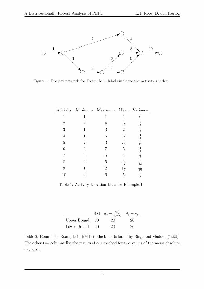
These two examples perfectly illustrate the quality of the bound on the expected
project duration we obtain. In example 1, where previous known bounds determine the
expected project duration exactly, irrespective of the true distribution, we find the exact
same value. We note that in this example there is only a single critical path for all
scenarios, which is why the best- and worst-case project duration coincide.
In example 2, on the other hand, there are multiple potential critical paths. The lower
and upper bounds found by Birge and Maddox (1995) therefore still had a significant
gap. Here, we can narrow the gap by a factor three if we know (or have an accurate
estimate of) the mean absolute deviation. Moreover, if only the variance is known, we
can tighten the bounds to [3.07, 3.68], which is still a little over half the original gap. This
empirically shows that the bounds by Birge and Maddox (1995) are not tight. We note
that for illustrative purposes, the potential deviation in these examples is unrealistically
large (up to 100% of the mean). The relative size of the gap with respect to the value of
the expected project duration is therefore disproportionally large.
10
A Distributionally Robust Analysis of PERT E.J. Roos, D. den Hertog
1
2
3
4
5
6
7
8
9
10
Figure 1: Project network for Example 1, labels indicate the activity’s index.
Acitivity Minimum Maximum Mean Variance
1 1 1 1 0
2 2 4 3 13
3 1 3 2 13
4 1 5 3 43
5 2 3 212
112
6 3 7 5 43
7 3 5 4 13
8 4 5 412
112
9 1 2 112
112
10 4 6 5 13
Table 1: Activity Duration Data for Example 1.
BM de = 2σ2e
be−ae de = σe
Upper Bound 20 20 20
Lower Bound 20 20 20
Table 2: Bounds for Example 1. BM lists the bounds found by Birge and Maddox (1995).
The other two columns list the results of our method for two values of the mean absolute
deviation.
11

A Distributionally Robust Analysis of PERT E.J. Roos, D. den Hertog
1
23
4
5
Figure 2: Project network for Example 2, labels indicate the activity’s index.
Acitivity Minimum Maximum Mean Variance
1 0 2 1 23
2 0 2 1 23
3 0 2 1 23
4 0 2 1 23
5 0 2 1 23
Table 3: Activity Duration Data for Example 2.
BM de = 2σ2e
be−ae de = σe
Upper Bound 4 3.36 3.68
Lower Bound 3 3.07 3.31
Table 4: Bounds for Example 2. BM lists the bounds found by Birge and Maddox (1995).
The other two columns list the results of our method for two values of the mean absolute
deviation.
12
A Distributionally Robust Analysis of PERT E.J. Roos, D. den Hertog
5.2 PSPLIB Instances
To test our approach on a larger scale, we use the RCPSP problems from the PSPLIB
project scheduling library (Kolisch and Sprecher, 1997). This library contains a wealth
of problems with m = 30, 60, 90 and 120 activities. We need to adapt these instances to
make them fully suitable for our approach. First and foremost, the problems are modeled
as an activity on nodes (AoN) network. To transform the projects into the desirable
activity on arc (AoA) format, we employ the algorithm by (Sterboul and Wertheimer,
1981) as explained by (Mouhoub et al., 2011).
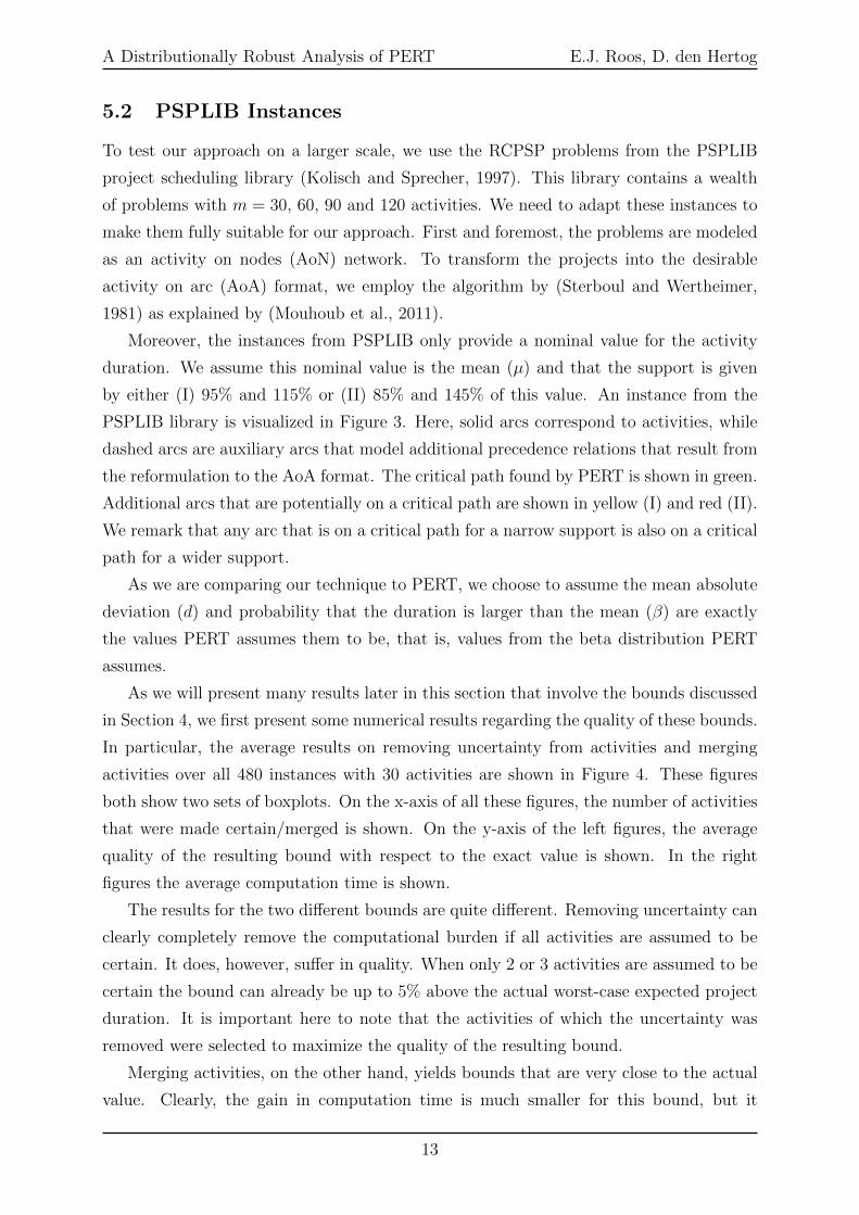
Moreover, the instances from PSPLIB only provide a nominal value for the activity
duration. We assume this nominal value is the mean (µ) and that the support is given
by either (I) 95% and 115% or (II) 85% and 145% of this value. An instance from the
PSPLIB library is visualized in Figure 3. Here, solid arcs correspond to activities, while
dashed arcs are auxiliary arcs that model additional precedence relations that result from
the reformulation to the AoA format. The critical path found by PERT is shown in green.
Additional arcs that are potentially on a critical path are shown in yellow (I) and red (II).
We remark that any arc that is on a critical path for a narrow support is also on a critical
path for a wider support.
As we are comparing our technique to PERT, we choose to assume the mean absolute
deviation (d) and probability that the duration is larger than the mean (β) are exactly
the values PERT assumes them to be, that is, values from the beta distribution PERT
assumes.
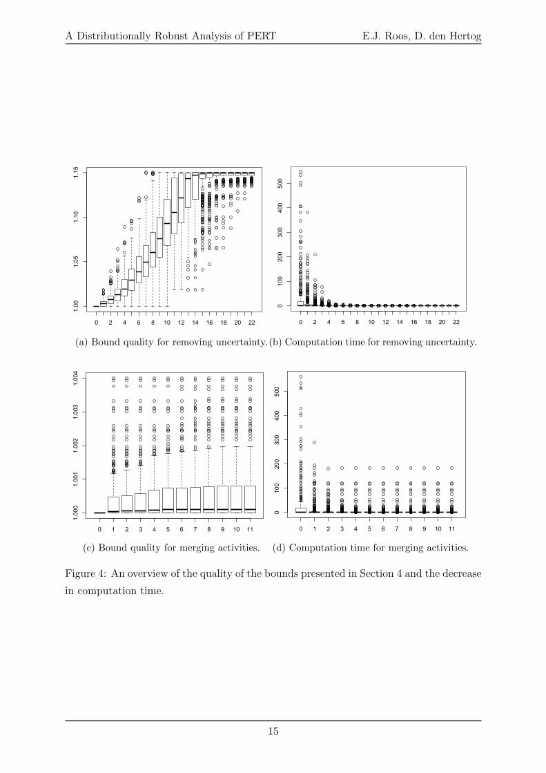
As we will present many results later in this section that involve the bounds discussed
in Section 4, we first present some numerical results regarding the quality of these bounds.
In particular, the average results on removing uncertainty from activities and merging
activities over all 480 instances with 30 activities are shown in Figure 4. These figures
both show two sets of boxplots. On the x-axis of all these figures, the number of activities
that were made certain/merged is shown. On the y-axis of the left figures, the average
quality of the resulting bound with respect to the exact value is shown. In the right
figures the average computation time is shown.
The results for the two different bounds are quite different. Removing uncertainty can
clearly completely remove the computational burden if all activities are assumed to be
certain. It does, however, suffer in quality. When only 2 or 3 activities are assumed to be
certain the bound can already be up to 5% above the actual worst-case expected project
duration. It is important here to note that the activities of which the uncertainty was
removed were selected to maximize the quality of the resulting bound.
Merging activities, on the other hand, yields bounds that are very close to the actual
value. Clearly, the gain in computation time is much smaller for this bound, but it
13

A Distributionally Robust Analysis of PERT E.J. Roos, D. den Hertog
Figure 3: A visualization of j301 2.sm. Solid arcs correspond to activities, dashed arcs
are auxiliary arcs. Green, yellow and red arcs correspond to activities on the critical path
for PERT, support I and support II, respectively.
14
A Distributionally Robust Analysis of PERT E.J. Roos, D. den Hertog
0 2 4 6 8 10 12 14 16 18 20 22
1.00
1.05
1.10
1.15
(a) Bound quality for removing uncertainty.
0 2 4 6 8 10 12 14 16 18 20 22
0100
200
300
400
500
(b) Computation time for removing uncertainty.
0 1 2 3 4 5 6 7 8 9 10 11
1.000
1.001
1.002
1.003
1.004
(c) Bound quality for merging activities.
0 1 2 3 4 5 6 7 8 9 10 11
0100
200
300
400
500
(d) Computation time for merging activities.
Figure 4: An overview of the quality of the bounds presented in Section 4 and the decrease
in computation time.
15

A Distributionally Robust Analysis of PERT E.J. Roos, D. den Hertog
is generally sufficient to tackle all problems with 30 activities and most with 60. We
therefore will limit ourselves to only consider this bound moving forward.
The best- and worst-case expected project duration for all 480 instances with 30
activities are shown for both values of the support (I and II) in Figures 5 and 6. For all
instances, the values of interest were divided by the expected project duration found by
PERT. The resulting fractions were grouped by and averaged over the instances that have
the same number of different critical paths. The images show the following four values:
• Best-case expected project duration without MAD known (equal to PERT) in blue;
• Best-case expected project duration with MAD known in green;
• Worst-case expected project duration with MAD known in yellow;
• Worst-case expected project duration without MAD known in red.
Figure 5 shows that on average, even in the most extreme projects, the difference between
the worst- and best-case expected project duration does not exceed 2%. Moreover, when
the mean-absolute deviation is known, the difference is significantly smaller. Note that this
is the difference between the green and yellow dots. In fact, the biggest difference between
the worst- and best-case expected project duration when the mean-absolute deviation is
known is slightly less than 3%. As we allow the activity duration to be up to 15% higher
than on average, and the support width is 20% of the mean value, we feel this 3% is rather
small. We therefore tentatively conclude that knowing the actual distribution (and mean
absolute deviation) has little influence on the expected project duration.
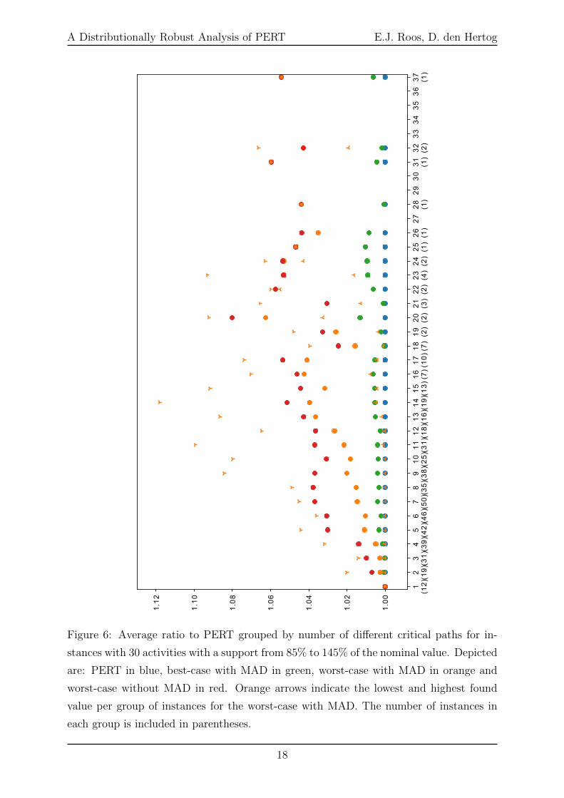
To investigate whether knowledge of the support does significantly change the ex-
pected project duration, Figure 6 shows the results when the activity duration is between
85% and 145% of its mean. As mentioned before, assuming a wider support implies that
more activities are potentially on the critical path. The number of relevant activities
thus increases and with it the computation time does as well. Hence, for a fair num-
ber of instances the exact worst- and best-case expected project duration could not be
calculated within 5 minutes. Therefore, we included a bound on those values based on
merging activities for those instances. While the difference to PERT is clearly bigger for
a larger support, the change seems mostly proportional to the change in the width of the
support. This strengthens our belief that knowledge of the support and mean is much
more important than knowledge of the actual distribution or the mean absolute deviation.
Appendix C contains similar figures to Figure 5 for projects with 60, 90 and 120
activities and a support from 95% to 115% of the mean: Figures 7, 8 and 9. For these sizes,
we randomly selected 50 instances from PSPLIB in order to prevent the total computation
time from becoming entirely unreasonable. While for both 90 and 120 activities there
16

A Distributionally Robust Analysis of PERT E.J. Roos, D. den Hertog
1(148)
2(128)
3(90)
4(50)
5(25)
6(16)
7(13)
8(4)
9(1)
10(2)
11(1)
12(2)
1.000
1.005
1.010
1.015
1.020
1.025
Figure 5: Average ratio to PERT grouped by number of different critical paths for in-
stances with 30 activities with a support from 95% to 115% of the nominal value. Depicted
are: PERT in blue, best-case with MAD in green, worst-case with MAD in yellow and
worst-case without MAD in red. Yellow arrows indicate the lowest and highest found
value per group of instances for the worst-case with MAD. The number of instances in
each group is included in parentheses.
17
A Distributionally Robust Analysis of PERT E.J. Roos, D. den Hertog
1(12)2(19)3(31)4(39)5(42)6(46)7(50)8(35)9(38)10
(25)11
(31)12
(18)13
(16)14
(19)15
(13)16(7)17
(10)18(7)19(2)20(2)21(3)22(2)23(4)24(2)25(1)26(1)2728(1)293031(1)32(2)3334353637(1)
1.00
1.02
1.04
1.06
1.08
1.10
1.12
Figure 6: Average ratio to PERT grouped by number of different critical paths for in-
stances with 30 activities with a support from 85% to 145% of the nominal value. Depicted
are: PERT in blue, best-case with MAD in green, worst-case with MAD in orange and
worst-case without MAD in red. Orange arrows indicate the lowest and highest found
value per group of instances for the worst-case with MAD. The number of instances in
each group is included in parentheses.
18
A Distributionally Robust Analysis of PERT E.J. Roos, D. den Hertog
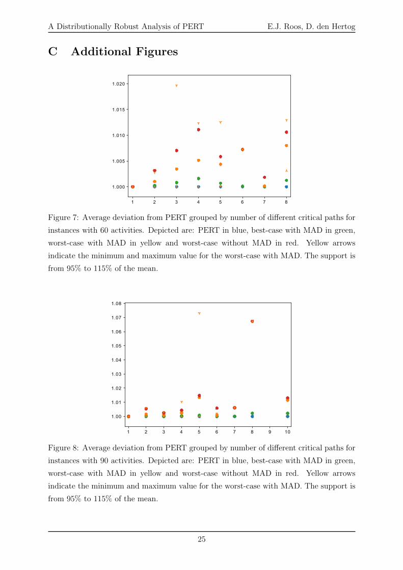
clearly exist some instances for which the difference between worst- and best-case expected
project duration is bigger, on average the difference is still fairly small. Moreover, we
remark that due to the size of these instances all results presented here have the maximum
number of activities merged that was possible. The true difference, therefore, is likely to
be at least somewhat smaller than the figures suggest.
Acknowledgments
The research of the first author was funded by the Netherlands Organisation for Scientific
Research (NWO) Research Talent [Grant 406.17.511].
References
Bard, J. F. and Bennett, J. E. (1991). Arc reduction and path preference in stochastic acyclic
networks. Management Science, 37(2):198–215.
Ben-Tal, A. and Hochman, E. (1972). More bounds on the expectation of a convex function of
a random variable. Journal of Applied Probability, 9(4):803–812.
Birge, J. R. and Maddox, M. J. (1995). Bounds on expected project tardiness. Operations
Research, 43(5):838–850.
Demassey, S., Artigues, C., and Michelon, P. (2005). Constraint-propagation-based cutting
planes: An application to the resource-constrained project scheduling problem. INFORMS
Journal on Computing, 17(1):52–65.
Hahn, E. D. (2008). Mixture densities for project management activity times: A robust approach
to pert. European Journal of Operational Research, 188(2):450–459.
Hajdu, M. (2013). Effects of the application of activity calendars on the distribution of project
duration in pert networks. Automation in Construction, 35:397–404.
Johnson, D. (1997). The triangular distribution as a proxy for the beta distribution in risk
analysis. Journal of the Royal Statistical Society: Series D (The Statistician), 46(3):387–398.
Klein Haneveld, W. K. (1986). Robustness against dependence in PERT: An application of
duality and distributions with known marginals. In Stochastic Programming 84 Part I, pages
153–182. Springer.
Kolisch, R. and Sprecher, A. (1997). PSPLIB - A project scheduling problem library: OR
Software - ORSEP Operations Research Software Exchange Program. European Journal of
Operational Research, 96(1):205–216.
19
A Distributionally Robust Analysis of PERT E.J. Roos, D. den Hertog
Kotiah, T. and Wallace, N. D. (1973). Another look at the pert assumptions. Management
Science, 20(1):44–49.
Littlefield Jr, T. and Randolph, P. (1987). Reply - an answer to Sasieni’s question on PERT
times. Management Science, 33(10):1357–1359.
Malcolm, D. G., Roseboom, J. H., Clark, C. E., and Fazar, W. (1959). Application of a technique
for research and development program evaluation. Operations Research, 7(5):646–669.
Mouhoub, N. E., Benhocine, A., and Belouadah, H. (2011). A new method for constructing a
minimal pert network. Applied Mathematical Modelling, 35(9):4575–4588.
Postek, K., Ben-Tal, A., Den Hertog, D., and Melenberg, B. (2018). Robust optimization
with ambiguous stochastic constraints under mean and dispersion information. Operations
Research, 66(3):814–833.
Reich, D. and Lopes, L. (2011). Preprocessing stochastic shortest-path problems with application
to pert activity networks. INFORMS Journal on Computing, 23(3):460–469.
Sterboul, F. and Wertheimer, D. (1981). Comment construire un graphe pert minimal. RAIRO-
Operations Research, 15(1):85–98.
Zhu, G., Bard, J. F., and Yu, G. (2006). A branch-and-cut procedure for the multimode resource-
constrained project-scheduling problem. INFORMS Journal on Computing, 18(3):377–390.
20

A Distributionally Robust Analysis of PERT E.J. Roos, D. den Hertog
A Algorithm Description
A basic implementation of the idea in Section 3 would be to store the longest path for every
scenario and iterate over all scenarios for which longest path remains to be unknown. This
approach, however, quickly runs into severe memory limitations, as for any graph with 21 or
more arcs, the number of stored scenarios would exceed the number of bytes available in a
computer with 4GB RAM.
Instead, Algorithm 1 stores the scenarios for which the longest path is already known in a
more intelligent way, enabling the algorithm to deal with even larger problems. In this algorithm,
remaining is a subroutine that computes the total probability of the scenarios induced by the
current scenario and critical path couple (α,C), of which the critical path was not yet known.
Here, induced scenarios refers to all scenarios α such thatαc = αc ∀c ∈ C
αc ≤ αc ∀c 6∈ C.
For ease of exposure, the algorithmic details given in Algorithm 2 and 3 concern two possible
values for each activity, as would be the case when calculating the best-case project duration.
With some minor modifications the algorithm can also be applied when an activity can take
more than three or more values.
The main algorithm iterates over a list of scenarios L, to which scenarios are added in many
iterations, until L is empty. For each scenario α, the longest path C in the corresponding graph
Algorithm 1
1: Set V = ∅2: Set L = {(2, . . . , 2)}3: Set i = 1
4: while L 6= ∅ do5: Choose α ∈ L and remove it from L
6: Compute λi = f(ν1α1, . . . , νmαm) and let C ⊆ A be the longest path of length l
7: Compute the total probability γi =∏c∈C p
cαc · remaining((α,C), V )
8: Add (α,C) to V
9: for all a ∈ C such that αa > 1 do
10: Define α by αa = αa − 1 and αc = αc for all c 6= a
11: if α 6∈ L & 6 ∃C such that (α,C) ∈ V then
12: Add α to L
13: end if
14: end for
15: Increase i by 1
16: end while
17: The worst-case expected project length is given by γ>λ.
21

A Distributionally Robust Analysis of PERT E.J. Roos, D. den Hertog
Algorithm 2 remaining subroutine
1: function remaining ((α,C), V )
2: Define V(α,C) ={α : ∃(α, C) ∈ V for which C = C, αc = αc ∀c ∈ C
}3: if V(α,C) = ∅ then4: Set ω =
∏c 6∈C
∑αci=1 p
ci
5: else
6: Set ω = 0
7: for all c 6∈ C such that αc > αc ∀α ∈ V(α,C) do
8: Update ω = ω +
[∑αci=maxα∈V(a,C)
{αc}+1 pci
]·∏χ 6∈C∪{c}
∑αχi=1 p
χi
9: Update αc = maxα αc
10: end for
11: Update ω = ω + recursive((α,C), V(α,C), ∅)12: end if
13: end function
is computed. Based on this longest path and the observation above, the induced set of scenarios
arises for which we now know the project length. Using the remaining subroutine, the total
probability of all scenarios of which we did not know the project length before is calculated.
Subsequently, a new scenario α is created for each arc on the longest path that is not set to
its lowest possible value, by lowering the value on said arc. Given that the scenarios that this
yields have not yet been considered, they are added to L.
The remaining subroutine first reduces all previously considered scenarios to the relevant
ones, that is, it selects the scenarios with the same critical path and the same activity durations
on this critical path. If such scenarios do not exist, all scenarios induced by α are new and
calculation of the total probability is easy. If such scenarios do exist, on the other hand, the
calculation is split into two parts. First of all, we check if any arc c not on the critical path has
a higher value than what has been considered before. For all such activity c, we can be sure
that any scenarios induced by α for which the value on c is equal are new scenarios and can
thus be included in the total probability. For the second part of the calculation, all arc lengths
are reduced to the maximum value that was considered before this iteration and the recursive
subroutine recursive is called.
First and foremost, recursive checks whether the scenario under consideration is dominated
by any scenario processed before. In this case, α does not induce any scenario we have not
encountered before and thus the remaining probability is 0. Otherwise, we find all activities i
such that we have considered scenarios before that had higher values on every activity but i and
add those to a set F . The value of these activities must remain fixed, as lowering them would
result in duplicate scenarios. After this, we can reduce the set of relevant previous scenarios to
all scenarios such that their value exceeds the value of α on all activities in F , as those are fixed
on their current value. This reduced set is denoted by V . If only 1 or none of such scenarios
22

A Distributionally Robust Analysis of PERT E.J. Roos, D. den Hertog
Algorithm 3 recursive subroutine
1: function recursive ((α,C), V, F0)
2: if ∃α ∈ V such that αc ≥ αc ∀c 6∈ C then
3: return 0
4: else
5: Set F = {i 6∈ C : ∃α ∈ V such that αi < αi, αc ≥ αc ∀c 6∈ C ∪ F0 ∪ {i}} ∪ F0
6: if |F | > 0 then
7: Set V = {α ∈ V : αc ≥ αc ∀c ∈ F}8: else
9: Set V = V
10: end if
11: if |V | ≤ 1 then
12: if |V | = 0 then
13: return∏c∈F p
cαc ·
∏c 6∈C∪F
∑αci=1 p
ci
14: else
15: Denote the only element of F by χ
16: Set B = {c 6∈ C : χc < αc}17: return
∏c∈F p
cαc ·
[∏c∈B
∑αci=1 p
ci −
∏c∈B
∑χci=1 p
ci
]·∏c 6∈C∪F∪B
∑αci=1 p
ci
18: end if
19: else
20: Find an arc j such that j 6∈ F and αj > 0
21: Define F1 = F ∪ {j} and V1 = {α ∈ V : αc ≥ αc ∀c ∈ F1}22: Define α by αj = αj − 1 and αc = αc for all c 6= j
23: return recursive((α,C), V1, F1) + recursive((α, C), V , F )
24: end if
25: end if
26: end function
exist, calculating the total probability of all new induced scenarios is fairly straightforward. If,
on the other hand, more than 1 scenario reside in V , we consider two cases for which we compute
the total probability of induced scenarios recursively. More specifically, we choose an activity
that is not fixed and not at its lowest value and consider the case where this activity is in fact
fixed and the case where its value is lower.
23
A Distributionally Robust Analysis of PERT E.J. Roos, D. den Hertog
B Project Preprocessing
Besides intelligently calculating the project duration for relevant scenarios, another observation
is key in efficiently evaluating the worst-case expected project duration. If there exists a node
k ∈ {1, . . . , n} such that for each scenario α the longest path in the corresponding graph contains
k, the expected project duration is equal to the sum of the expected longest path from 1 to k
and the expected longest path from k to n. In other words, if there exists a node that is on any
longest path, irrespective of the activity duration, it suffices to find the worst-case longest path
from 1 to k and the worst-case longest path from k to n. This observation is valid because we
assume all activity lengths to be independent. We will refer to nodes k with the above property
as separating nodes.
Unfortunately, these separating nodes are not necessarily easy to identify. When any path
from 1 to n passes through k, that is, removing k from the graph would disconnect it completely,
it is clear that k is a separating node. The easiest way to identify all other separating nodes is
removing all edges from the graph that are never contained in a longest path from 1 to n. A
computationally expensive, but intuitive to find these edges is to compute supP∈Pµ E [f(l)]. Since
the worst-case distribution for this ambiguity set is only a two-point distribution on the bound-
aries of the support, any edge that is not on the longest path for any of the considered scenarios
in this evaluation, will not be on any longest path. Calculating supP∈Pµ E [f(l)] first can thus
yield a significant decrease in computation time of supP∈P(µ,d)E [f(l)] and infP∈P(µ,d,β)
E [f(l)].
A more computationally tractable approach to identify separating nodes is to apply the
following sufficient but not necessary condition. First we note that the shortest possible longest
path has length f(a). Now, for any edge (i, j) ∈ A we find the longest possible path from 1
to n containing this edge. Then we know that (i, j) is never in a longest path if this length is
strictly smaller than f(a). We once again stress that although this is a sufficient condition, it is
not necessary.
By first checking the sufficient condition outlined above and subsequently computing the
values of interest in the order indicated, that is computing supP∈Pµ E [f(l)] first, we can limit
the graph to only the relevant edges fairly efficiently, thereby identifying all separating nodes.
More efficient and elaborate techniques for reducing the project of interest exist. As our
implementation only serves an illustrative purpose, we chose not to implement those even though
we suspect using such techniques could improve the applicability of our techniques even further.
We refer the interested reader to e.g. (Bard and Bennett, 1991; Reich and Lopes, 2011).
24
A Distributionally Robust Analysis of PERT E.J. Roos, D. den Hertog
C Additional Figures
1 2 3 4 5 6 7 8
1.000
1.005
1.010
1.015
1.020
Figure 7: Average deviation from PERT grouped by number of different critical paths for
instances with 60 activities. Depicted are: PERT in blue, best-case with MAD in green,
worst-case with MAD in yellow and worst-case without MAD in red. Yellow arrows
indicate the minimum and maximum value for the worst-case with MAD. The support is
from 95% to 115% of the mean.
1 2 3 4 5 6 7 8 9 10
1.00
1.01
1.02
1.03
1.04
1.05
1.06
1.07
1.08
Figure 8: Average deviation from PERT grouped by number of different critical paths for
instances with 90 activities. Depicted are: PERT in blue, best-case with MAD in green,
worst-case with MAD in yellow and worst-case without MAD in red. Yellow arrows
indicate the minimum and maximum value for the worst-case with MAD. The support is
from 95% to 115% of the mean.
25

A Distributionally Robust Analysis of PERT E.J. Roos, D. den Hertog
1 2 3 4 5 6 7 8 9 10 11 12 13 14 15 16
1.00
1.02
1.04
1.06
1.08
1.10
Figure 9: Average deviation from PERT grouped by number of different critical paths
for instances with 120 activities. Depicted are: PERT in blue, best-case with MAD in
green, worst-case with MAD in yellow and worst-case without MAD in red. Yellow arrows
indicate the minimum and maximum value for the worst-case with MAD. The support is
from 95% to 115% of the mean.
26