a discontinuous-galerkin-based extended finite element ... · a discontinuous-galerkin-based...

NSF GRANT # 0747089NSF PROGRAM NAME: Immersed BoundaryMethods in Computational Solid Mechanics

A Discontinuous-Galerkin-based Extended Finite Element Method forFracture Mechanics: Immersed Boundary Perspective and Optimal

Convergence

Adrian LewDepartment of Mechanical Engineering, Stanford University

Yongxing ShenDepartment of Mechanical Engineering, Stanford University

Abstract: The extended finite element method (XFEM)enables the representation of cracks in arbitrary locationsof a mesh. We introduce here a variant of the XFEM ren-dering an optimally convergent scheme. Its distinguish-ing features are: a) the introduction of singular asymptoticcrack tip fields with support on only a small region aroundthe crack tip, the enrichment region, b) only one and twoenrichment functions are added for anti-plane shear andplanar problems, respectively, and c) the relaxation of thecontinuity between the enrichment region and the rest ofthe domain, and the adoption of a discontinuous Galerkin(DG) method therein. The method is provably stable forany positive value of a stabilization parameter.

1 Introduction: Fracture mechanics plays an essentialrole in failure analysis of engineering structures. Accu-rately and efficiently computing the stress field is crucialfor predicting the evolution of cracks. In fracture mechan-ics problems, cracks are usually idealized as geometries ofone less dimension than that of the embedding solid, i.e.,submanifolds of codimension 1. This idealization givesrise to a stress singularity of the type1/

√r for isotropic

linear elastic materials, wherer is the distance to the cracktip, and leads to suboptimal convergence rates if standardfinite element methods (FEMs) with piecewise polyno-mial spaces are employed.

There are virtually two families of strategies toachieve better convergence behavior: adaptive mesh re-finement and extension of the finite element (FE) spacewith thea priori known singular functions. This introduc-tion will focus on developments along the second familyof the aforementioned methods.

With minimal alteration to existing FE programs,Henshell and Shaw [1] and Barsoum [2] independentlyproposed using isoparametric 8-noded quadrilateral ele-

ments while placing some of the mid-side nodes at thequarter positions so as to produce the

√r behavior of the

displacement field in the physical domain. The quarter-point elements are straightforward to implement. How-ever, the singularity they introduced in the FE space doesnot capture the angular dependence of the strain field nearthe crack tip. Consequently, even though convergence isstill attained and the accuracy of the solution is enhanced,there is no improvement in the convergence rate with re-spect to FE discretizations with standard elements; it re-mains suboptimal.

In 1973, Fix et al. [3] introduced singular functionsin combination with standard piecewise polynomial func-tions for solving Poisson and Helmholtz equations overa cracked domain. The singular functions are continu-ous and have compact supports centered at the singularity(crack tip). However, they are non-local, which meansthat their support spans many elements in the mesh. Infact, the support of the singular functions is the same re-gardless of the mesh size. By doing so, they obtained anoptimal convergence rate and accurate approximations tothe stress intensity factors (SIFs).

More recently Belytschko and Black [4] and Moeset al. [5] introduced the extended finite element method(XFEM), in which they adopted a partition of unity (PU)technique [6, 7] to incorporate the singularities into theFE basis. Its key advantage is that it requires minimalor no remeshing as the crack propagates. In this contexta typical enrichment shape function is the product of asingular function and a standard, continuous, piecewisepolynomial shape function. In the early developments ofthe XFEM, only elements adjacent to (or very close to)the crack tip were enriched with the singular functions.

Since the introduction of the XFEM applied to frac-ture mechanics problems, related literature grew rapidly,

Proceedings of 2011 NSF Engineering Research and Innovation Conference, Atlanta, Georgia GRANT # 0747089

and numerous variants of the XFEM have been proposed.In 2003, Chessa et al. [8] observed the suboptimal con-vergence rate of the then standard XFEMs, and attributedthis phenomenon to the presence of blending elements,i.e., enriched elements bordering standard elements. LaterLaborde et al. [9] and Bechet et al. [10] showed that ifthe size of the enrichment zone shrinks around the crackash → 0 then the convergence rate will be suboptimal.Hence, they proposed enriching elements over a fixed areaindependent of the mesh.

A number of strategies has been proposed to over-come the suboptimal convergence rate due to the pres-ence of blending elements. The authors in [8] proposedtwo methods for removing this artifact: a) adding a bub-ble quadratic function to the blending elements and b) us-ing the assumed strain method. Another method that stilladopted a PU to include the singular enrichment and cor-rected the suboptimal convergence rate due to the blend-ing elements was proposed by Fries [11]. The author mul-tiplied each singular enrichment basis function by a cut-off function that increases from zero to one in a singlering of elements, the transition layer. While normally thisproduct would have very large derivatives in the transitionlayer, the particular choices of enrichment functions havesmall derivatives therein, leading to optimal convergencerate in the numerical examples.

Generalizing the original ideas in [3], Chahine etal. [12, 13] overcame the problem of blending elementsby multiplying the singular enrichment functions by asmooth cutoff function independent of the mesh size. Theauthors also proved the optimal convergence rate of thismethod.

In [9] the authors framed the problem of the blendingelements as one of approximating a function in two over-lapping domains, the domains with and without enrich-ment functions, through a PU approach. It follows fromtheir analysis that the convergence rate should not be af-fected as the width of the overlapping region, or transitionlayer, decreases to zero. Consequently, in this limit thistype of method would require the approximations on bothsides of the interface between the domains with and with-out enrichment functions to be essentially continuous,i.e., discontinuities are allowed but these should becomesmaller and smaller as the mesh is refined. The authorsthen proposed to introduce a basis for the singular enrich-ment functions without the PU technique, which they la-beled “degree of freedom gathering,” and then match thenodal values of the numerical solutions along the interfacebetween the domains with and without enrichment func-tions.

An idea that is strongly related to those in the previous

paragraph is to include the singular enrichment functionson a region that contains the crack tip, and set them to zerooutside this region. The resulting enrichment functionsare discontinuous at the interface between the two regions,and hence a discontinuous Galerkin (DG) approximationcan be adopted therein to weakly enforce continuity. Thiswas proposed in [14], where the authors combined thePU-based XFEM and the interior penalty DG methods in[15] and [16]. One drawback of this approach is that sta-bilization is required, and the stabilization parameter isproblem dependent. A few iterations are needed to find asuitable value.

The idea of introducing discontinuities to weakly en-force continuity of non-polynomial basis functions canalso be found in Farhat et al. [17] and Massimi et al.[18] for wave propagation problems, and Yuan and Shu[19] for convection-diffusion problems. In [17] and [18],weak continuity is restored by introducing Lagrange mul-tipliers along the element boundaries, while in [19] this isaccomplished through a local DG method.

In this paper we propose a new DG method to connectsolutions on the domains with and without enrichmentfunctions. The method is based on the DG methods forelastic problems in [20] and [21], which are constructedby adopting the Bassi-Rebay numerical fluxes. An impor-tant feature of this class of methods is that for isotropic,unstressed, linear elastic problems the stabilization termis problem independent. In fact, it is enough for the stabi-lization parameter to be any positive real number.

Another important feature of the method is that onlythe two asymptotic displacement fields near the crack tipfor modes I and II are adopted as enrichment functions.This enables us to compute the SIF for each mode sim-ply as the coefficient of the enrichment basis function inthe numerical solution. We show the convergence of thesecoefficients to their exact values through numerical exam-ples. While the rate of convergence of the SIFs computedin this way is lower than those computed through the inter-action integral [5], the resulting values are surprisinglyac-curate and require essentially no extra computational cost.Among the methods that introduce enrichments by multi-plying by a PU basis, the one by Liu et al. [22] also ex-tracts the SIFs as the coefficients of the enrichment basisfunctions.

To retain an optimal order of convergence, we set thedomain over which the singular enrichment functions arenot zero to be the set of all elements that intersect a circlewhose radius is independent ofh. Consequently, the num-ber of elements over which the enrichment functions aredifferent than zero scales ash−2. For arbitrary enrichmentfunctions this would mean that the number of nonzero en-


tries in the stiffness matrix relating the enrichment func-tions with the polynomial basis functions scales ash−2

as well. However, because the enrichment basis functionsare in mechanical equilibrium, we show that most of theseentries are identically zero. In fact, the number of suchnon-zero entries scales ash−1, which renders the stiff-ness matrix surprisingly sparse. Only a polynomial basisfunction whose support includes either the boundary ofthe enrichment region or a portion of the face of a curvedcrack would couple to the enrichment functions through anon-zero pair of entries in the stiffness matrix.

We demonstrate the optimal convergence propertiesof the method with numerical examples. We comparethe results against those obtained by adopting the cutofffunction approach [13], since the authors proved that thismethod attains an optimal convergence rate. For the samemesh, the errors in stresses, displacements and SIFs aresubstantially lower for the method proposed herein. Thesedifferences are not expected to be large if compared withother methods that set the enrichment functions to zerowith either a zero-width transition layer as in Laborde etal. [9], or a shrinking transition layer ash tends to zero asin Fries [11], but we did not perform such comparison.

Finally, in Section 2.2 we construct a connection be-tween immersed boundary methods (see, e.g., [23]) andthe XFEM by representing the crack path as an immersedboundary rather than an additional enrichment. This per-spective is similar but not identical to those introducedby Molino et al. [24], Song et al. [25] and Hansbo andHansbo [26]. This point of view simplifies the construc-tion of FE spaces over cracked domains, such as spacesof arbitrary polynomial order or with different degrees ofcontinuity across element boundaries (DG, conforming,Raviart-Thomas elements, etc.).

In this paper we denote with‖ · ‖L2(B) and| · |H1(B)

theL2-norm andH1-seminorm overB, respectively.

2 Methodology:

2.1 Problem statement: We consider the two-dimensional linear elastostatic problem over a boundedopen polygonal domainΩ ∈ R2. It reads findu : Ω → R2

such that

−∇ · (C : ∇u) = f , in Ω,

u = U , on ∂dΩ,

(C : ∇u) · n = T , on ∂τΩ,

(1)

wheref : Ω → R2 is the body force,n is the exteriorunit normal to∂Ω, ∂dΩ ∪ ∂τΩ = ∂Ω, ∂dΩ ∩ ∂τΩ = ∅,T : ∂Ωτ → R2 are the imposed tractions andU : ∂dΩ →

R2 are the imposed displacements. The elastic moduliC

are those of an initially stress-free isotropic material.In particular, we are interested in problems in which

Ω is a domain with cracks. Each crack is assumed to be asmooth one-dimensional curve. Additionally, we assumethat there exists an open neighborhood of each crack suchthat a) the open neighborhoods of two different cracks donot intersect and, b) once the open neighborhood of eachcrack or any of its subsets has been removed fromΩ, aconnected domain remains. These assumptions precludethe important possibilities of intersecting cracks, such asa bifurcation, and of crack kinks. While some of theseconfigurations do not need further modifications of themethod to retain an optimal convergence rate, some ofthem do. We therefore restrict our attention to a less gen-eral setting, so as to convey the key new ideas in the sim-plest terms.

We shall make the standard assumption that crackfaces are traction free, i.e.,T = 0 on∂crΩ ⊆ ∂τΩ, where∂crΩ is the set of crack faces. In this way we rule outcontact and friction between crack faces.

We assume thatC is constant throughout the do-main, or at least, in the open neighborhood around eachcrack tip. Generalizations that retain an optimal rate ofconvergence to smoothly spatially varying moduli, or toanisotropic materials, are possible provided an asymp-totic displacement field near each crack tip is known un-der those circumstances, and of course, some regularityconditions for the solution are met.

For simplicity, we shall explain the method assumingthat there is only one crack tip whose position is denotedby xt, which means we consider an edge crack. The gen-eralization to multiple crack tips is trivial.

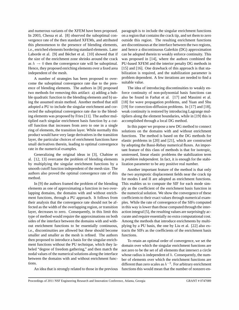
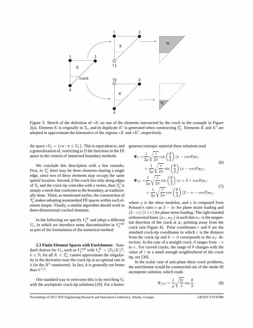
Following Stolarska et al. [27], we assume that thereexist smooth scalar functionsφ andg overΩ such that thecrack is contained in the level setφ = 0, and along thecrackg is strictly monotonous withg(xt) = 0. The crackis then defined as∂crΩ = x ∈ Ω : φ(x) = 0, g(x) < 0,see Figure 2(a). By construction,xt /∈ ∂crΩ.

2.2 Crack Paths as Immersed Boundaries:Adopt-ing the philosophy of the XFEM, we construct a familyof quasi-uniform triangulationsThh of Ω parametrizedby the mesh sizeh > 0. We do so without taking intoaccount the locations of the cracks. Therefore we allowfor the possibility of the crack cutting through elements.We assume that any node in meshTh either belongs to thecrack or is a distance ofǫh away from any point on thecrack for someǫ > 0 independent ofh. This conditionprevents the crack from cutting elements into arbitrarilysmall parts, which would render poorly conditioned stiff-


ness matrices. Additionally, we henceforth assume thatelements are open subsets ofΩ, and that the intersectionof the crack∂crΩ and any elementK can only be eitheran empty set or a connected curve, for anyK in Thh.In other words, if any elementK is cut by the crack atall, it can only be cut into at most two parts. A similarbut not identical assumption was made in [26], becausethey followed a convention in which elements are treatedas closed sets.

In this paper we adopt the distinct perspective ofcracks as immersed boundaries. This perspective is ofcourse equivalent to regarding them as jump discontinu-ities in the deformation mapping, as in the XFEM. How-ever, it leads to a simple and elegant implementation ofthe method. Furthermore, this perspective simplifies theconstruction of enriched FE spaces in cracked domainswith a variety of elements, not only of the conformingP1

type. Similar albeit not identical ideas have been intro-duced by Molino et al. [24], Song et al. [25] and Hansboand Hansbo [26].

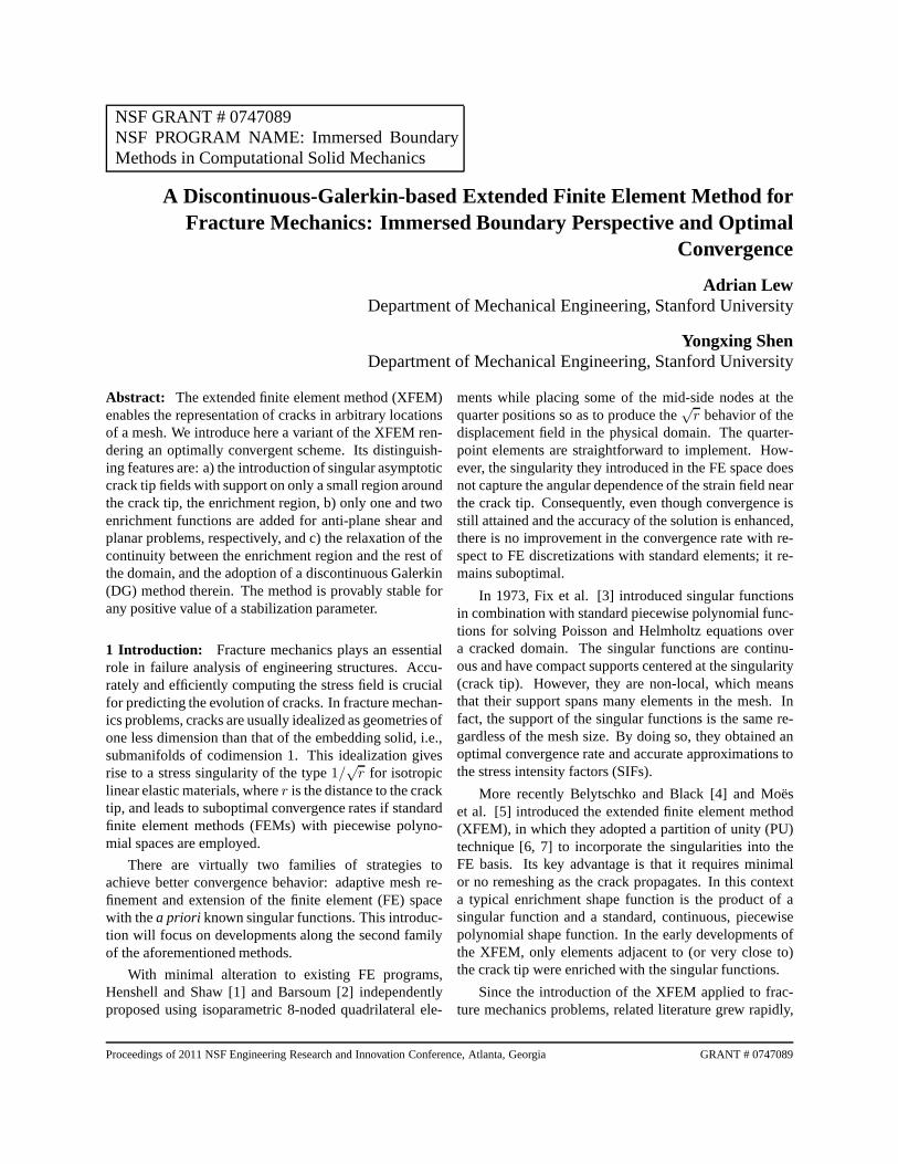
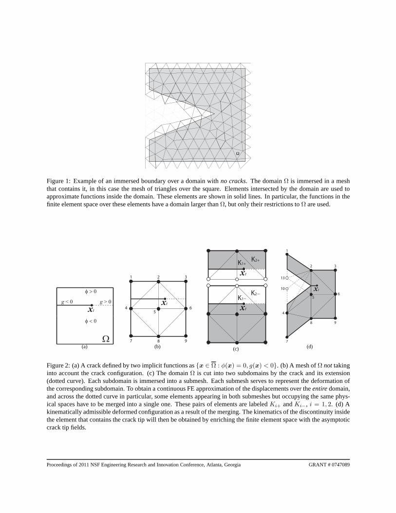
In immersed boundary methods the domainΩ is over-lapped over a mesh that does not fit the boundary, see e.g.[23]. In this way,∂Ω cuts through elements in the mesh,see Figure 1 for an example over a domain withno cracks.A FE spaceVh can be easily constructed over all elementsintersected byΩ. However, only the restriction of func-tions inVh to Ω is important for the approximate solution.

A crack is clearly part of the boundary ofΩ. However,in contrast to the example in Figure 1, when immersingΩinto Th some elements intersectΩ on both sides of thecrack. Consequently, if the basis functions within the ele-ment are continuous, then the kinematics on the two sidesof the crack are artificially connected. This artifact can benaturally avoided with a simple modification ofTh that in-volves duplicating some nodes and elements to constructa new meshT ′

h.The basic idea can be explained by splitting the mesh

along a curve that contains the crack into two discon-nected ones, and then “gluing” them back together alongthe non-cracked part of this curve, see Figure 2. This sep-aration into two steps is not needed for the final algorithm,but is introduced to facilitate the explanation. In fact, thecriteria of duplication are

ElementK is duplicated⇔K \ ∂crΩ is not connected,

Nodea is duplicated⇔cloud(a) \ ∂crΩ is not connected,

wherecloud(a) is defined as the interior of the closure ofthe domain occupied by all elements inTh that havea asa node (the cloud of a nodea is also the interior of the

support of the standard piecewise linear shape functionassociated with nodea).

We developed a precise algorithm in [28] that is ableto construct a new meshT ′

h with duplicated elements froma meshTh for the uncracked solid. The new meshT ′

h haselements that occupy the same location in space. How-ever, each one of the two copies can be adopted to describethe kinematics of only one side of the crack, effectivelytreating each crack face as a regular immersed boundary.

OnceT ′h is defined, a FE spaceVh can be defined over

it such that

Vh ⊆∏

K∈T ′

h

V Kh

=

v =(

vK1, . . . ,vK

N′

)

: vK ∈ V Kh , ∀K ∈ T ′

h

(2)whereV K

h is the FE space over elementK andN ′ is thetotal number of elements inT ′

h. For example, a standardchoice would be a space that contains functions that arecontinuous across elements that share a common edge,i.e., elements that have two nodes in common. In thiscase,

V confh =

v ∈∏

K∈T ′

h

V Kh : vK |e = vK′ |e

if K,K ′ share edgee, for anye

.

(3)

Notice thatVh may contain functions that are bi-valued over some regions of the domain. In particular,these will be bi-valued over the domain of all elementsK ∈ Th that have been duplicated when constructingT ′

h.To specify which of these two values shall be used to ap-proximate the solution of the problem, we define

∗K =

K \ ∂crΩ if K was not duplicated

K ∩ Ω± if K was duplicated andit shares a node with an element

K ∈ T ′h such thatK ⊂ Ω±,

(4)for any elementK ∈ T ′

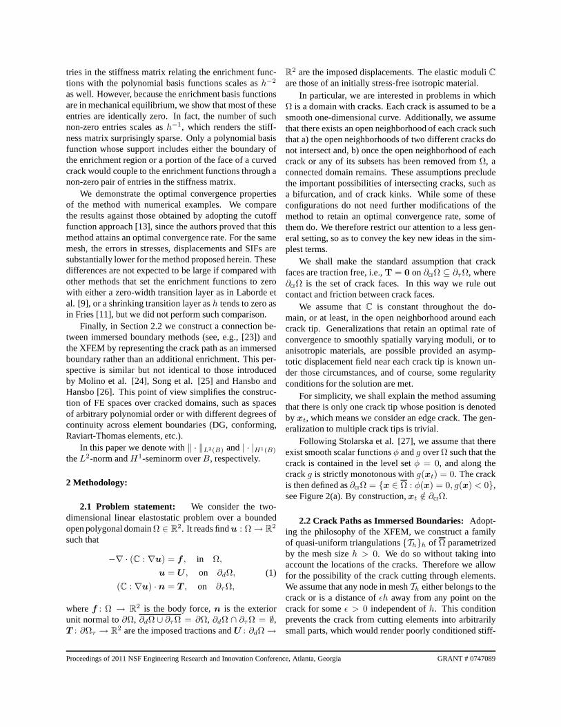
h, see Figure 3 for a sketch. Eachv ∈ Vh then defines a function∗v overΩ (up to a set ofmeasure zero) such that

∗v|∗K = v|∗K (5)

for all K ∈ T ′h. The resulting function∗v is single-

valued almost everywhere inΩ. Roughly speaking,∗vis obtained fromv by restricting its values to the “half” ofthe element that does not contain duplicated nodes, for allthose elements that are completely cut by the crack. Ap-proximation of solutions will then be effectively sought in


Ω

Figure 1: Example of an immersed boundary over a domain withno cracks. The domainΩ is immersed in a meshthat contains it, in this case the mesh of triangles over the square. Elements intersected by the domain are used toapproximate functions inside the domain. These elements are shown in solid lines. In particular, the functions in thefinite element space over these elements have a domain largerthanΩ, but only their restrictions toΩ are used.

xt

Ω

φ > 0

φ < 0

g > 0g < 0

(a)

xt

1 2 3

45

6

7 8 9

(b)

xt

K1+K2+

xt

K1

K2_

_

(c)

xt

1

2 3

7

8 9

56

4

10

13

(d)

Figure 2: (a) A crack defined by two implicit functions asx ∈ Ω : φ(x) = 0, g(x) < 0. (b) A mesh ofΩ not takinginto account the crack configuration. (c) The domainΩ is cut into two subdomains by the crack and its extension(dotted curve). Each subdomain is immersed into a submesh. Each submesh serves to represent the deformation ofthe corresponding subdomain. To obtain a continuous FE approximation of the displacements over theentiredomain,and across the dotted curve in particular, some elements appearing in both submeshes but occupying the same phys-ical spaces have to be merged into a single one. These pairs ofelements are labeledKi+ andKi−, i = 1, 2. (d) Akinematically admissible deformed configuration as a result of the merging. The kinematics of the discontinuity insidethe element that contains the crack tip will then be obtainedby enriching the finite element space with the asymptoticcrack tip fields.


1 2

4

10 2

4

1 2

13K

K

K’

*K

*K’

crack

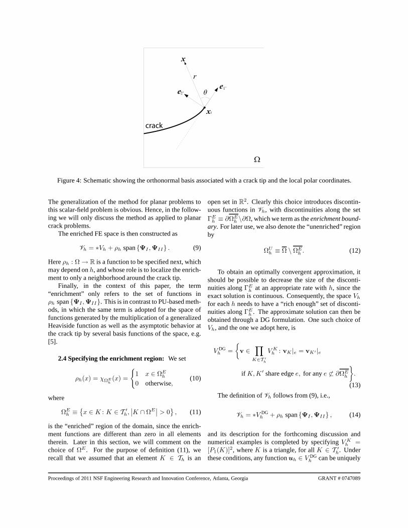
Figure 3: Sketch of the definition of∗K on one of the elements intersected by the crack in the examplein Figure2(a). ElementK is originally inTh, and its duplicateK ′ is generated when constructingT ′

h. ElementsK andK ′ areadopted to approximate the kinematics of the regions∗K and∗K ′, respectively.

the space∗Vh = ∗v : v ∈ Vh. This is equivalent to, anda generalization of, restricting toΩ the functions in the FEspace in the context of immersed boundary methods.

We conclude this description with a few remarks.First, in T ′

h there may be three elements sharing a singleedge, since two of these elements may occupy the samespatial location. Second, if the crack lies only along edgesof Th and the crack tip coincides with a vertex, thenT ′

h issimply a mesh that conforms to the boundary, as tradition-ally done. Third, as mentioned earlier, the construction ofT ′

h makes adopting nonstandard FE spaces within each el-ement simple. Finally, a similar algorithm should work inthree-dimensional cracked domains.

In the following we specifyV Kh and adopt a different

Vh, in which we introduce some discontinuities inV confh

as part of the formulation of the numerical method.

2.3 Finite Element Spaces with Enrichment: Stan-dard choices forVh, such asV conf

h with V Kh = [Pk(K)]2,

k ∈ N, for all K ∈ T ′h, cannot approximate the singular-

ity in the derivative near the crack tip at an optimal rate inh (in theH1-seminorm). In fact, it is generally not betterthanh1/2.

One standard way to overcome this is by enrichingVh

with the asymptotic crack-tip solutions [29]. For a homo-

geneous isotropic material these solutions read

ΨI =1

2µ

√

r

2πcos

(

θ

2

)

(κ− cos θ)e1′

+1

2µ

√

r

2πsin

(

θ

2

)

(κ− cos θ)e2′ ,

(6)

ΨII =1

2µ

√

r

2πsin

(

θ

2

)

(κ+ 2 + cos θ)e1′

+1

2µ

√

r

2πcos

(

θ

2

)

(2 − κ− cos θ)e2′ ,

(7)

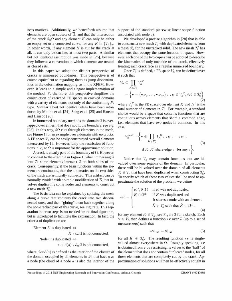
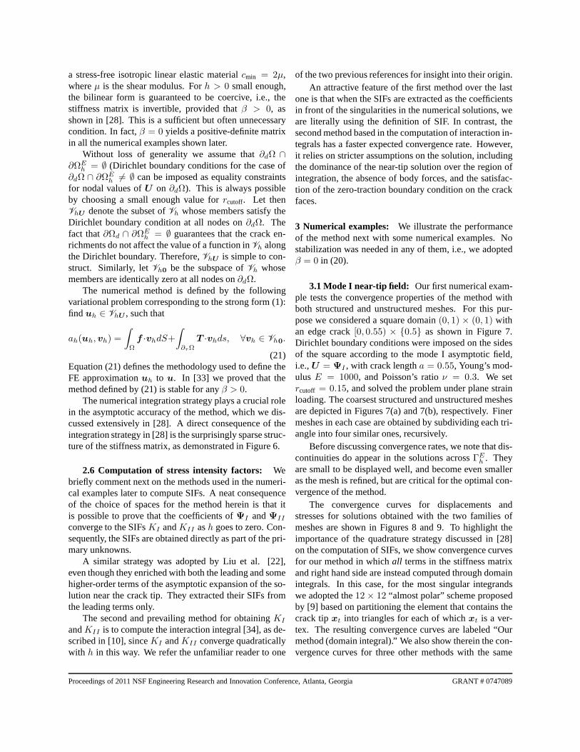
whereµ is the shear modulus, andκ is computed fromPoisson’s ratioν as3 − 4ν for plane strain loading and(3−ν)/(1+ν) for plane stress loading. The right-handedorthonormal basise1′ , e2′ is such thate1′ is the tangen-tial direction of the crack atxt pointing away from thecrack (see Figure 4). Polar coordinatesr andθ are thestandard crack-tip coordinates in whichr is the distancefrom the crack tip andθ = 0 corresponds to thee1′ di-rection. In the case of a straight crack,θ ranges from−πto π. For curved cracks, the range ofθ changes with thevalue ofr in a small enough neighborhood of the cracktip, see [30].

In the scalar case of anti-plane shear crack problems,the enrichment would be constructed out of the mode IIIasymptotic solution, which reads

ΨIII =1

µ

√

2r

πsin

θ

2. (8)


x

r

ee

crack

xt

θ1’

2’

Ω

Figure 4: Schematic showing the orthonormal basis associated with a crack tip and the local polar coordinates.

The generalization of the method for planar problems tothis scalar-field problem is obvious. Hence, in the follow-ing we will only discuss the method as applied to planarcrack problems.

The enriched FE space is then constructed as

Vh = ∗Vh + ρh spanΨI ,ΨII . (9)

Hereρh : Ω → R is a function to be specified next, whichmay depend onh, and whose role is to localize the enrich-ment to only a neighborhood around the crack tip.

Finally, in the context of this paper, the term“enrichment” only refers to the set of functions inρh spanΨI ,ΨII. This is in contrast to PU-based meth-ods, in which the same term is adopted for the space offunctions generated by the multiplication of a generalizedHeaviside function as well as the asymptotic behavior atthe crack tip by several basis functions of the space, e.g.[5].

2.4 Specifying the enrichment region: We set

ρh(x) = χΩE

h

(x) =

1 x ∈ ΩEh

0 otherwise,(10)

where

ΩEh ≡

x ∈ K : K ∈ T ′h,∣

∣K ∩ ΩE∣

∣ > 0

, (11)

is the “enriched” region of the domain, since the enrich-ment functions are different than zero in all elementstherein. Later in this section, we will comment on thechoice ofΩE . For the purpose of definition (11), werecall that we assumed that an elementK ∈ Th is an

open set inR2. Clearly this choice introduces discontin-uous functions inVh, with discontinuities along the setΓE

h ≡ ∂ΩEh \∂Ω, which we term as theenrichment bound-

ary. For later use, we also denote the “unenriched” regionby

ΩUh ≡ Ω \ ΩE

h . (12)

To obtain an optimally convergent approximation, itshould be possible to decrease the size of the disconti-nuities alongΓE

h at an appropriate rate withh, since theexact solution is continuous. Consequently, the spaceVh

for eachh needs to have a “rich enough” set of disconti-nuities alongΓE

h . The approximate solution can then beobtained through a DG formulation. One such choice ofVh, and the one we adopt here, is

V DGh =

v ∈∏

K∈T ′

h

V Kh : vK |e = vK′ |e

if K,K ′ share edgee, for anye 6⊂ ∂ΩEh

.

(13)

The definition ofVh follows from (9), i.e.,

Vh = ∗V DGh + ρh spanΨI ,ΨII , (14)

and its description for the forthcoming discussion andnumerical examples is completed by specifyingV K

h =[P1(K)]2, whereK is a triangle, for allK ∈ T ′

h. Underthese conditions, any functionuh ∈ V DG

h can be uniquely


expressed as

uh = χΩU

h

∑

a∈SU

2∑

i=1

ψauUaiei

+ χΩE

h

(

∑

a∈SE

2∑

i=1

ψauEaiei +KIΨI +KIIΨII

)

,

(15)whereKI , KII , uE

ai are scalars,χB denotes the charac-teristic function of domainB, andSE andSU denote thesets of nodes in elements included inΩE

h andΩUh , respec-

tively. Functionψa is such thatψa|K is aP1 function foreachK ∈ T ′

h, continuous across elements that share anedge, and equal to1 at a and zero on every other nodein T ′

h. By construction,uh may be discontinuous acrossΓE

h , and possibly bi-valued on elements and edges that in-tersect the crack∂crΩ. In contrast,∗uh is single-valuedtherein, and possibly discontinuous across∂crΩ.

Choice ofΩE : As ΩE we choose the intersection ofΩ with an open disk centered at the crack tip with radiusrcutoff > 0. We assume thatrcutoff is such thatΩE

h ∩ ∂crΩis a connected curve for any meshTh. This conditionprevents the crack from reentering the enrichment region.Since the hypotheses in Section 2 prevent the crack fromintersecting itself, it is always possible to choosercutoff

such that forh small enough a ball of radiusrcutoff + hcentered at the crack tip (which containsΩE

h ) intersectsthe crack in a connected curve only. Furthermore, we as-sume thatTh is such that∂crΩ ∩ ΓE

h contains at most onepoint. This is clearly not satisfied for all meshes, since thecrack may overlap with (parts of) edges inΓE

h . However,it can be accomplished by slightly perturbing the positionof only a few nodes providedh is small enough. This lastassumption is not essential, but it greatly simplifies theimplementation of the method. An example ofΩE andthe resultingΩE

h are shown in Figure 5.

2.5 Discontinuous Galerkin method for the enrich-ment boundary: The approximation of continuous so-lutions with possibly-discontinuous functions needs thecraft of special numerical methods, such as one of themany variants of DG methods. The reader is referred toArnold et al. [31] for a unified analysis of many variantsof DG methods. The method proposed herein originatesin the one constructed for linear elastic problems in [20],and for the Poisson equation in [32].

We first define some notation. Letn be the outwardunit normal toΩE

h , i.e., pointing towardsΩUh . For a scalar,

vector or tensor fieldv overΩ we denote withvE andvU

its traces onΓEh from ΩE

h andΩUh , respectively. We also

define the jump and average operators onΓEh as

JvK ≡ vE − vU , v ≡ 1

2

(

vE + vU)

, (16)

We note that different authors have adopted differentconventions for defining these operators, especially forvectorial arguments (see, for example, Arnold et al. [31]).Here we define them in a way that scalars, vectors andtensor fields are treated alike. Additionally, since we shallstrongly impose Dirichlet boundary conditions, there is noneed to define these operators on∂Ω.

Definition of the DG-derivative: Following a stan-dard approach in some DG methods (see e.g., [21, 31]),approximations of the derivative of the solution are con-structed through a DG-derivative operator on the discon-tinuous displacement field. This is defined asDDG :Vh → (L2(Ω))2×2 as

DDGvh = ∇vh + R(JvhK) in K, for anyK ∈ T ′h,

(17)where the (right) lifting operatorR :

(

L2(

ΓEh

))2 →Wh ⊂ (L2(Ω))2×2 is a linear operator that maps a dis-placement jump acrossΓE

h to a strain defined overΩ suchthat for each elementK ∈ T ′

h∫

Ω

R(vh) : γh dS = −∫

ΓE

h

vh · γh · n ds,

∀γh ∈ Wh,

(18)

where

Wh ≡

γh ∈∏

K∈T ′

h

WKh :

WKh = (P1(∗K))2×2 if ∗K ⊂ ΩU

h ,

andWKh = (P2(∗K))2×2 if ∗K ⊂ ΩE

h

.

(19)Here Pk(K), for k a nonnegative integer, denotes thefunction space consisting of polynomials of degree up tok overK.

Variational Principle: Having definedDDG, we in-troduce the following bilinear formah(·, ·) : Vh × Vh →R:

ah(uh,vh) ≡∑

K∈T ′

h

∫

∗K

DDGuh : C : DDGvh dS

+ β cmin

∫

Ω

R(JuhK) : R(JvhK) dS,

(20)whereβ ∈ R is a stabilization parameter, andcmin is theminimum eigenvalue ofC among symmetric strains. For


xt

∂crΩ ΩE

ΩE

ΓE

rcutoff

h

h

Figure 5: Specification of the enrichment regionΩE using a circle. Elements in dark gray are enriched with the near-tip asymptotic displacement fields. Their union isΩE

h . Discontinuities in the displacement field are introduced across

the boundary ofΩEh , in this case alsoΓE

h , to cutoff the enrichment fields while retaining an optimal convergence rate.A DG formulation is adopted along the elements with an edge alongΓE

h , which includes the elements shown in lightgray outsideΩE

h . Some elements may have more than one of its edges across which discontinuities are allowed, as theone shown with a hollow square. Other elements may be both intersected by the crack and have an edge intersectedby ΓE

h . In this example those are shown with a black circle. These elements come in pairs, one for the kinematics oneach side of the crack. In one of these pairs only one of the twoelements shares an edge withΓE

h .


a stress-free isotropic linear elastic materialcmin = 2µ,whereµ is the shear modulus. Forh > 0 small enough,the bilinear form is guaranteed to be coercive, i.e., thestiffness matrix is invertible, provided thatβ > 0, asshown in [28]. This is a sufficient but often unnecessarycondition. In fact,β = 0 yields a positive-definite matrixin all the numerical examples shown later.

Without loss of generality we assume that∂dΩ ∩∂ΩE

h = ∅ (Dirichlet boundary conditions for the case of∂dΩ ∩ ∂ΩE

h 6= ∅ can be imposed as equality constraintsfor nodal values ofU on ∂dΩ). This is always possibleby choosing a small enough value forrcutoff. Let thenVhU denote the subset ofVh whose members satisfy theDirichlet boundary condition at all nodes on∂dΩ. Thefact that∂Ωd ∩ ∂ΩE

h = ∅ guarantees that the crack en-richments do not affect the value of a function inVh alongthe Dirichlet boundary. Therefore,VhU is simple to con-struct. Similarly, letVh0 be the subspace ofVh whosemembers are identically zero at all nodes on∂dΩ.

The numerical method is defined by the followingvariational problem corresponding to the strong form (1):find uh ∈ VhU , such that

ah(uh,vh) =

∫

Ω

f ·vhdS+

∫

∂τΩ

T ·vhds, ∀vh ∈ Vh0.

(21)Equation (21) defines the methodology used to define theFE approximationuh to u. In [33] we proved that themethod defined by (21) is stable for anyβ > 0.

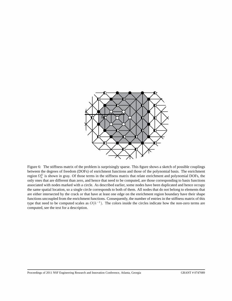
The numerical integration strategy plays a crucial rolein the asymptotic accuracy of the method, which we dis-cussed extensively in [28]. A direct consequence of theintegration strategy in [28] is the surprisingly sparse struc-ture of the stiffness matrix, as demonstrated in Figure 6.

2.6 Computation of stress intensity factors: Webriefly comment next on the methods used in the numeri-cal examples later to compute SIFs. A neat consequenceof the choice of spaces for the method herein is that itis possible to prove that the coefficients ofΨI andΨII

converge to the SIFsKI andKII ash goes to zero. Con-sequently, the SIFs are obtained directly as part of the pri-mary unknowns.

A similar strategy was adopted by Liu et al. [22],even though they enriched with both the leading and somehigher-order terms of the asymptotic expansion of the so-lution near the crack tip. They extracted their SIFs fromthe leading terms only.

The second and prevailing method for obtainingKI

andKII is to compute the interaction integral [34], as de-scribed in [10], sinceKI andKII converge quadraticallywith h in this way. We refer the unfamiliar reader to one

of the two previous references for insight into their origin.An attractive feature of the first method over the last

one is that when the SIFs are extracted as the coefficientsin front of the singularities in the numerical solutions, weare literally using the definition of SIF. In contrast, thesecond method based in the computation of interaction in-tegrals has a faster expected convergence rate. However,it relies on stricter assumptions on the solution, includingthe dominance of the near-tip solution over the region ofintegration, the absence of body forces, and the satisfac-tion of the zero-traction boundary condition on the crackfaces.

3 Numerical examples: We illustrate the performanceof the method next with some numerical examples. Nostabilization was needed in any of them, i.e., we adoptedβ = 0 in (20).

3.1 Mode I near-tip field: Our first numerical exam-ple tests the convergence properties of the method withboth structured and unstructured meshes. For this pur-pose we considered a square domain(0, 1) × (0, 1) withan edge crack[0, 0.55) × 0.5 as shown in Figure 7.Dirichlet boundary conditions were imposed on the sidesof the square according to the mode I asymptotic field,i.e.,U = ΨI , with crack lengtha = 0.55, Young’s mod-ulusE = 1000, and Poisson’s ratioν = 0.3. We setrcutoff = 0.15, and solved the problem under plane strainloading. The coarsest structured and unstructured meshesare depicted in Figures 7(a) and 7(b), respectively. Finermeshes in each case are obtained by subdividing each tri-angle into four similar ones, recursively.

Before discussing convergence rates, we note that dis-continuities do appear in the solutions acrossΓE

h . Theyare small to be displayed well, and become even smalleras the mesh is refined, but are critical for the optimal con-vergence of the method.

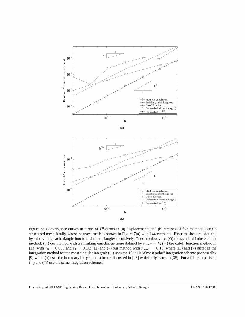
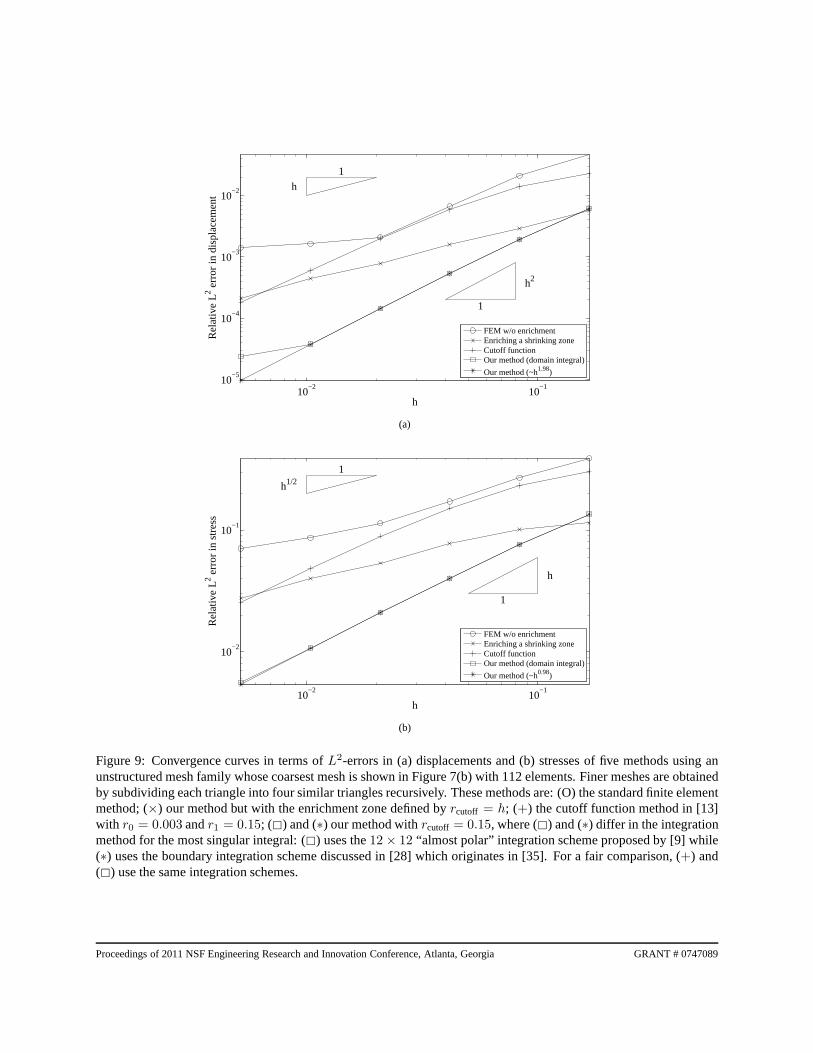
The convergence curves for displacements andstresses for solutions obtained with the two families ofmeshes are shown in Figures 8 and 9. To highlight theimportance of the quadrature strategy discussed in [28]on the computation of SIFs, we show convergence curvesfor our method in whichall terms in the stiffness matrixand right hand side are instead computed through domainintegrals. In this case, for the most singular integrandswe adopted the12 × 12 “almost polar” scheme proposedby [9] based on partitioning the element that contains thecrack tipxt into triangles for each of whichxt is a ver-tex. The resulting convergence curves are labeled “Ourmethod (domain integral).” We also show therein the con-vergence curves for three other methods with the same


b

Figure 6: The stiffness matrix of the problem is surprisingly sparse. This figure shows a sketch of possible couplingsbetween the degrees of freedom (DOFs) of enrichment functions and those of the polynomial basis. The enrichmentregionΩE

h is shown in gray. Of those terms in the stiffness matrix that relate enrichment and polynomial DOFs, theonly ones that are different than zero, and hence that need tobe computed, are those corresponding to basis functionsassociated with nodes marked with a circle. As described earlier, some nodes have been duplicated and hence occupythe same spatial location, so a single circle corresponds toboth of them. All nodes that do not belong to elements thatare either intersected by the crack or that have at least one edge on the enrichment region boundary have their shapefunctions uncoupled from the enrichment functions. Consequently, the number of entries in the stiffness matrix of thistype that need to be computed scales asO(h−1). The colors inside the circles indicate how the non-zero terms arecomputed, see the text for a description.


meshes, namely: a) the (standard) FEM that results fromchoosingVh = ∗V conf

h , in which no singular enrichmentsare included, b) our method with the quadrature strategyin [28] but with a shrinking enrichment zone, i.e., wechose a differentΩE for eachh by settingrcutoff = hmax

wherehmax is the maximum length among all trianglesin each mesh, see Section 2.4, and c) the cutoff functionmethod by [13] withr0 = 0.003 andr1 = 0.15, see Sec-tion 2.4 as well. In (c) all integrals were performed overthe domain by using the strategy in [9], as we did for thecurves labeled “Our method (domain integral).”

These results show that not including singular enrich-ments, or including them but only in an enrichment zonethat shrinks withh gives rise to the same type of subop-timal convergence rate. Naturally, errors in the latter caseare smaller, as seen in Figures 8 and 9. Both the cutofffunction method and our method render an apparent op-timal convergence rate. However, for this example theerrors with the method introduced herein are uniformlysmaller by roughly one order of magnitude. For this rangeof mesh sizes there is no distinguishable difference be-tween the quadrature strategies, except for the data pointin Figure 9(a) corresponding to the finest mesh. As wediscuss next, this is no longer the case when the conver-gence of the SIFs is considered.

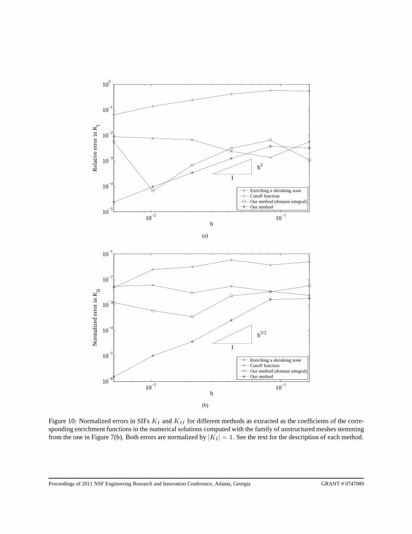
Figure 10 shows the errors in modes I and II SIFs ex-tracted as the coefficients of the enrichment basis func-tionsΨI andΨII , respectively, for each one of the meth-ods for which this is possible. When endowed with thequadrature strategy in [28], our method displays a remark-able ability to capture the value of the SIFs as the meshis refined, in this and subsequent examples. In contrast,when endowed with the domain integration scheme de-scribed in [9], the SIFs do not display a converging pat-tern. The reasons behind this behavior can be traced backto the lack of an appropriate order for the consistency er-ror introduced by the quadrature rule. On the other hand,the cutoff function method which also uses a domain inte-gration scheme does show a converging trend for the SIFsas the mesh is refined, at least forKI , but the errors of thismethod are larger for the same mesh and cutoff radius ofenrichment.

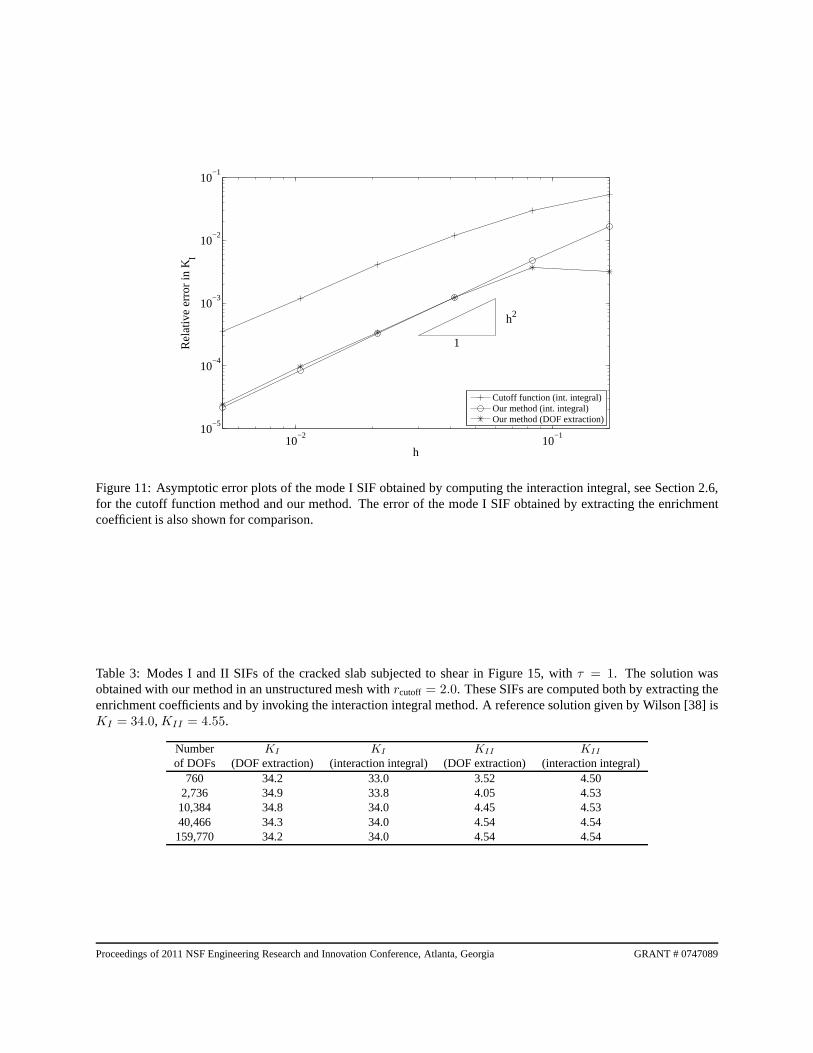
We next compare the convergence of the SIF in modeI when computed with the interaction integral, see Figure11. Quadratic convergence is attained for our method aswell as the cutoff function method, with the former havingan error approximately one order of magnitude smaller forthe same mesh. Also plotted is the SIF extracted as the co-efficient ofΨI in our method. In this case the two meth-ods of extracting SIFs yield very similar results. However,in general the convergence rate of the method based on the

interaction integral will be faster, though more computa-tionally expensive as well.

Finally, we investigated the dependence of the error inthe stress field and the mode I SIF as the value ofrcutoff ischanged for our method. These values were computed onan unstructured mesh obtained by performing one subdi-vision of that in Figure 7(b). A comparison with the cutofffunction method is also shown, by varying the value ofr1and keeping either the ratior0/r1 or the value ofr0 fixed.The results are shown in Figure 12, indicating as expectedthat the largerrcutoff is, the smaller the errors become.

3.2 Uniaxial tension: In this second numerical ex-ample we compute the SIF of a planar slab with a crackof lengtha in plane strain under uniaxial tension, i.e., thetraction vector on the faces parallel to the crack is normalto them and has magnitudeσ, as shown in Figure 13(a).The Young’s modulus and Poisson’s ratio are 1000 and0.3, respectively. The deformed configuration obtainedwith a relatively fine mesh, together with a contour plot ofthe von Mises stress is shown in Figure 13(b).

The mode I SIF for this example is given by Tada etal. [36] as

KI = σ√Wf

( a

W

)

, (22)

whereW denotes the width of the plate and

f( a

W

)

=

√

2 tan πa2W

cos πa2W

×[

0.752 + 2.02a

W+ 0.37

(

1 − sinπa

2W

)3]

.

(23)

In Table 1, we have tabulated the computed values ofKI comparing the results reported in Stazi et al. [30] andthose of our method with a structured mesh similar to theone in Figure 7(a) andrcutoff = 0.15W . Both results arethen obtained with comparable meshes, approximately thesame number ofP1 DOFs. Regardless of howKI is com-puted, either directly from the DOF conjugate toΨI orthrough the interaction integral, the values computed withthe method herein are closer to the exact ones.

3.3 Mixed-mode loadings: Our next two examplesare two mixed-mode loadings: a planar slab with a slantededge crack subject to uniaxial tension, see Figure 14, andanother one in which one side is clamped and another sideis subject to uniform shear, see Figure 15. The Young’smoduli and Poisson’s ratios are 1000 and 0.3 for the firstexample and 30 and 0.25 for the second example.

We solved these two problems with an unstructuredmesh similar to that shown in Figure 7(b). The computedSIFs are tabulated in Tables 2 and 3, respectively. Note


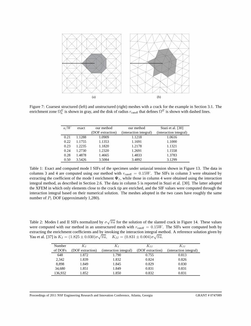
(a) (b)

Figure 7: Coarsest structured (left) and unstructured (right) meshes with a crack for the example in Section 3.1. Theenrichment zoneΩE

h is shown in gray, and the disk of radiusrcutoff that definesΩE is shown with dashed lines.

a/W exact our method our method Stazi et al. [30](DOF extraction) (interaction integral) (interaction integral)

0.21 1.1288 1.0909 1.1218 1.06160.22 1.1755 1.1353 1.1691 1.10000.23 1.2235 1.1820 1.2178 1.13210.24 1.2730 1.2320 1.2691 1.15580.28 1.4878 1.4665 1.4833 1.37830.50 3.5426 3.5084 3.4892 3.1299

Table 1: Exact and computed mode I SIFs of the specimen under uniaxial tension shown in Figure 13. The data incolumns 3 and 4 are computed using our method withrcutoff = 0.15W . The SIFs in column 3 were obtained byextracting the coefficient of the mode I enrichmentΨI , while those in column 4 were obtained using the interactionintegral method, as described in Section 2.6. The data in column 5 is reported in Stazi et al. [30]. The latter adoptedthe XFEM in which only elements close to the crack tip are enriched, and the SIF values were computed through theinteraction integral based on their numerical solution. The meshes adopted in the two cases have roughly the samenumber ofP1 DOF (approximately 1,280).

Table 2: Modes I and II SIFs normalized byσ√πa for the solution of the slanted crack in Figure 14. These values

were computed with our method in an unstructured mesh withrcutoff = 0.15W . The SIFs were computed both byextracting the enrichment coefficients and by invoking the interaction integral method. A reference solution given byYau et al. [37] isKI = (1.825 ± 0.030)σ

√πa, KII = (0.831± 0.004)σ

√πa.

Number KI KI KII KII

of DOFs (DOF extraction) (interaction integral) (DOF extraction) (interaction integral)648 1.872 1.790 0.755 0.813

2,342 1.839 1.832 0.824 0.8268,898 1.849 1.845 0.829 0.83034,680 1.851 1.849 0.831 0.831136,932 1.852 1.850 0.832 0.831


10−2

10−1

10−5

10−4

10−3

10−2

h

Rel

ativ

e L2 e

rror

in d

ispl

acem

ent

1

h2

1h

FEM w/o enrichmentEnriching a shrinking zoneCutoff functionOur method (domain integral)

Our method (~h1.99)

(a)

10−2

10−1

10−2

10−1

h

Rel

ativ

e L2 e

rror

in s

tres

s

1

h

1

h1/2


Our method (~h0.99)

(b)

Figure 8: Convergence curves in terms ofL2-errors in (a) displacements and (b) stresses of five methodsusing astructured mesh family whose coarsest mesh is shown in Figure 7(a) with 144 elements. Finer meshes are obtainedby subdividing each triangle into four similar triangles recursively. These methods are: (O) the standard finite elementmethod; (×) our method with a shrinking enrichment zone defined byrcutoff = h; (+) the cutoff function method in[13] with r0 = 0.003 andr1 = 0.15; () and (∗) our method withrcutoff = 0.15, where () and (∗) differ in theintegration method for the most singular integral: () uses the12×12 “almost polar” integration scheme proposed by[9] while (∗) uses the boundary integration scheme discussed in [28] which originates in [35]. For a fair comparison,(+) and () use the same integration schemes.


10−2

10−1

10−5

10−4

10−3

10−2

h

Rel

ativ

e L2 e

rror

in d

ispl

acem

ent

1

h2

1

h


Our method (~h1.98)

(a)

10−2

10−1

10−2

10−1

h

Rel

ativ

e L2 e

rror

in s

tres

s

1

h

1

h1/2


Our method (~h0.98)

(b)

Figure 9: Convergence curves in terms ofL2-errors in (a) displacements and (b) stresses of five methodsusing anunstructured mesh family whose coarsest mesh is shown in Figure 7(b) with 112 elements. Finer meshes are obtainedby subdividing each triangle into four similar triangles recursively. These methods are: (O) the standard finite elementmethod; (×) our method but with the enrichment zone defined byrcutoff = h; (+) the cutoff function method in [13]with r0 = 0.003 andr1 = 0.15; () and (∗) our method withrcutoff = 0.15, where () and (∗) differ in the integrationmethod for the most singular integral: () uses the12 × 12 “almost polar” integration scheme proposed by [9] while(∗) uses the boundary integration scheme discussed in [28] which originates in [35]. For a fair comparison, (+) and() use the same integration schemes.


10−2

10−1

10−5

10−4

10−3

10−2

10−1

100

h

Rel

ativ

e er

ror

in K I

1

h2

Enriching a shrinking zoneCutoff functionOur method (domain integral)Our method

(a)

10−2

10−1

10−6

10−5

10−4

10−3

10−2

10−1

h

Nor

mal

ized

err

or in

K II

1

h5/2

Enriching a shrinking zoneCutoff functionOur method (domain integral)Our method

(b)

Figure 10: Normalized errors in SIFsKI andKII for different methods as extracted as the coefficients of thecorre-sponding enrichment functions in the numerical solutions computed with the family of unstructured meshes stemmingfrom the one in Figure 7(b). Both errors are normalized by|KI | = 1. See the text for the description of each method.


10−2

10−1

10−5

10−4

10−3

10−2

10−1

h

Rel

ativ

e er

ror

in K I

1

h2

Cutoff function (int. integral)Our method (int. integral)Our method (DOF extraction)

Figure 11: Asymptotic error plots of the mode I SIF obtained by computing the interaction integral, see Section 2.6,for the cutoff function method and our method. The error of the mode I SIF obtained by extracting the enrichmentcoefficient is also shown for comparison.

Table 3: Modes I and II SIFs of the cracked slab subjected to shear in Figure 15, withτ = 1. The solution wasobtained with our method in an unstructured mesh withrcutoff = 2.0. These SIFs are computed both by extracting theenrichment coefficients and by invoking the interaction integral method. A reference solution given by Wilson [38] isKI = 34.0,KII = 4.55.

Number KI KI KII KII

of DOFs (DOF extraction) (interaction integral) (DOF extraction) (interaction integral)760 34.2 33.0 3.52 4.50

2,736 34.9 33.8 4.05 4.5310,384 34.8 34.0 4.45 4.5340,466 34.3 34.0 4.54 4.54159,770 34.2 34.0 4.54 4.54


0.05 0.1 0.15 0.2 0.25 0.3 0.35

10−1

rcutoff

Rel

ativ

e L2 e

rror

in s

tres

s

Cutoff function (fixed r0/r

1)

Cutoff function (fixed r0)

Our method

(a)

0.05 0.1 0.15 0.2 0.25 0.3 0.35

10−2

10−1

rcutoff

Rel

ativ

e er

ror

in K I

Cutoff function (fixed r0/r

1)

Cutoff function (fixed r0)

Our method

(b)

Figure 12: Relative errors in (a) stress and (b) mode I SIF as the value ofrcutoff is changed over the same mesh for ourmethod, or as the value ofr1 was changed for the cutoff function method. The SIF was extracted as the coefficient ofΨI . (O) cutoff function method withr0/r1 = 0.02; (×) cutoff function method withr0 = 0.003; (∗) our method.


(a) (b)

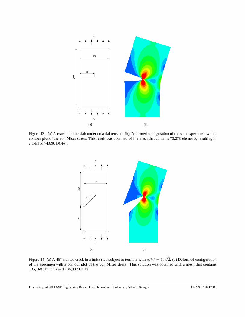
Figure 13: (a) A cracked finite slab under uniaxial tension. (b) Deformed configuration of the same specimen, with acontour plot of the von Mises stress. This result was obtained with a mesh that contains 73,278 elements, resulting ina total of 74,690 DOFs .

(a) (b)

Figure 14: (a) A45 slanted crack in a finite slab subject to tension, witha/W = 1/√

2. (b) Deformed configurationof the specimen with a contour plot of the von Mises stress. This solution was obtained with a mesh that contains135,168 elements and 136,932 DOFs.


(a) (b)

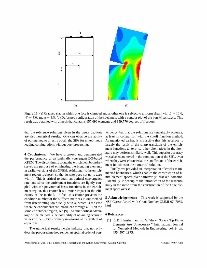
Figure 15: (a) Cracked slab in which one face is clamped and another one is subject to uniform shear, withL = 16.0,W = 7.0, anda = 3.5. (b) Deformed configuration of the specimen, with a contour plot of the von Mises stress. Thisresult was obtained with a mesh that contains 157,696 elements and 159,770 degrees of freedom.

that the reference solutions given in the figure captionsare also numerical results. One can observe the abilityof our method to directly obtain the SIFs for mixed-modeloading configurations without post-processing.

4 Conclusions: We have proposed and demonstratedthe performance of an optimally convergent DG-basedXFEM. The discontinuity along the enrichment boundaryserves the purpose of eliminating the blending elementsin earlier versions of the XFEM. Additionally, the enrich-ment region is chosen so that its size does not go to zerowith h. This is critical to attain an optimal convergencerate, and since the enrichment functions are lightly cou-pled with the polynomial basis functions in the enrich-ment region, this choice has a minor impact in the effi-ciency of the method. In fact, this choice prevents thecondition number of the stiffness matrices in our methodfrom deteriorating too quickly withh, which is the casewhen the enrichments are introduced through a PU on thesame enrichment region, see [9]. Another critical advan-tage of the method is the possibility of obtaining accuratevalues of the SIFs as primary unknowns of the system ofequations.

The numerical results herein indicate that not onlydoes the proposed method render an optimal order of con-

vergence, but that the solutions are remarkably accurate,at least in comparison with the cutoff function method.As mentioned earlier, it is possible that this accuracy islargely the result of the sharp transition of the enrich-ment functions to zero, so other alternatives in the liter-ature may perform similarly well. This superior accuracywas also encountered in the computation of the SIFs, evenwhen they were extracted as the coefficients of the enrich-ment functions in the numerical solution.

Finally, we provided an interpretation of cracks as im-mersed boundaries, which enables the construction of fi-nite element spaces over “arbitrarily” cracked domains.Essentially, it decouples the introduction of the disconti-nuity in the mesh from the construction of the finite ele-ment space over it.

5 Acknowledgements: This work is supported by theNSF Career Award with Grant Number CMMI-0747089.[39]

6 References:

[1] R. D. Henshell and K. G. Shaw, “Crack Tip FiniteElements Are Unnecessary,” International Journalfor Numerical Methods in Engineering, vol. 9, pp.495–507, 1975.


[2] R. S. Barsoum, “On the use of isoparametric fi-nite elements in linear fracture mechanics,” Interna-tional Journal for Numerical Methods in Engineer-ing, vol. 10, pp. 25–37, 1976.

[3] G. J. Fix, S. Gulati, and G. I. Wakoff, “On the useof singular functions with finite element approxima-tions,” Journal of Computational Physics, vol. 13,pp. 209–228, 1973.

[4] T. Belytschko and T. Black, “Elastic crack growthin finite elements with minimal remeshing,” Interna-tional Journal for Numerical Methods in Engineer-ing, vol. 45, pp. 601–620, 1999.

[5] N. Moes, J. Dolbow, and T. Belytschko, “A finite el-ement method for crack growth without remeshing,”International Journal for Numerical Methods in En-gineering, vol. 46, pp. 131–150, 1999.

[6] J. M. Melenk and I. Babuska, “The partition of unityfinite element method: basic theory and applica-tions,” Computer Methods in Applied Mechanicsand Engineering, vol. 139, pp. 289–314, 1996.

[7] I. Babuska and J. M. Melenk, “The partition of unitymethod,” International Journal for Numerical Meth-ods in Engineering, vol. 40, pp. 727–758, 1997.

[8] J. Chessa, H. Wang, and T. Belytschko, “On the con-struction of blending elements for local partion ofunity enriched finite elements,” International Jour-nal for Numerical Methods in Engineering, vol. 57,pp. 1015–1038, 2003.

[9] P. Laborde, Y. Renard, J. Pommier, and M. Salaun,“High Order Extended Finite Element Method ForCracked Domains,” International Journal for Nu-merical Methods in Engineering, vol. 64, pp. 354–381, 2005.

[10] E. Bechet, H. Minnebo, N. Moes, and B. Burgardt,“Improved implementation and robustness study ofthe X-FEM for stress analysis around cracks,” In-ternational Journal for Numerical Methods in Engi-neering, vol. 64, pp. 1033–1056, 2005.

[11] T.-P. Fries, “A corrected XFEM approximation with-out problems in blending elements,” InternationalJournal for Numerical Methods in Engineering,vol. 75, pp. 503–532, 2008.

[12] E. Chahine, P. Laborde, and Y. Renard, “A quasi-optimal convergence result for fracture mechanicswith XFEM,” C. R. Acad. Sci. Paris, Ser. I, vol. 342,2006.

[13] E. Chahine, P. Laborde, and Y. Renard, “Crack tipenrichment in the XFEM using a cutoff function,”International Journal for Numerical Methods in En-gineering, vol. 75, pp. 629–646, 2008.

[14] R. Gracie, H. Wang, and T. Belytschko, “Blendingin the extended finite element method by discontinu-ous Galerkin and assumed strain methods,” Interna-tional Journal for Numerical Methods in Engineer-ing, vol. 74, pp. 1645–1669, 2008.

[15] M. Wheeler, “An elliptic collocation-finite elementmethod with interior penalties,” SIAM Journal onNumerical Analysis, vol. 15, pp. 152–161, 1978.

[16] D. N. Arnold, “An interior penalty finite elementmethod with discontinuous elements,” SIAM Jour-nal on Numerical Analysis, vol. 19, pp. 742–760,1982.

[17] C. Farhat, I. Harari, and L. P. Franca, “The discon-tinuous enrichment method,” Computer Methods inApplied Mechanics and Engineering, vol. 190, pp.6455–6479, 2001.

[18] P. Massimi, R. Tezaur, and C. Farhat, “A discon-tinuous enrichment method for three-dimensionalmultiscale harmonic wave propagation problems inmulti-fluid and fluidsolid media,” International Jour-nal for Numerical Methods in Engineering, vol. 76,pp. 400–425, 2008.

[19] L. Yuan and C.-W. Shu, “Discontinuous Galerkinmethod based on non-polynomial approximationspaces,” Journal of Computational Physics, vol. 218,pp. 295–323, 2006.

[20] A. Lew, P. Neff, D. Sulsky, and M. Ortiz, “OptimalBV estimates for a discontinuous Galerkin methodfor linear elasticity,” Applied Mathematics ResearcheXpress, vol. 3, pp. 73–106, 2004.

[21] A. Ten Eyck and A. Lew, “Discontinuous Galerkinmethods for non-linear elasticity,” InternationalJournal for Numerical Methods in Engineering,vol. 67, pp. 1204–1243, 2006.

[22] X. Y. Liu, Q. Z. Xiao, and B. L. Karihaloo, “XFEMfor direct evaluation of mixed mode SIFs in ho-mogeneous and bi-materials,” International Journalfor Numerical Methods in Engineering, vol. 59, pp.1103–1118, 2004.


[23] A. J. Lew and G. C. Buscaglia, “A discontinuous-Galerkin-based immersed boundary method,” Inter-national Journal for Numerical Methods in Engi-neering, vol. 76, 2008.

[24] N. Molino, Z. Bao, and R. Fedkiw, “A virtual nodealgorithm for changing mesh topology during sim-ulation,” ACM Transactions on Graphics (TOG),vol. 23, pp. 385–392, 2004.

[25] J.-H. Song, P. M. A. Areias, and T. Belytschko, “Amethod for dynamic crack and shear band propa-gation with phantom nodes,” International Journalfor Numerical Methods in Engineering, vol. 67, pp.868–893, 2006.

[26] A. Hansbo and P. Hansbo, “An unfitted finite ele-ment method, based on Nitsche’s method, for ellipticinterface problems,” Computer Methods in AppliedMechanics and Engineering, vol. 191, pp. 5537–5552, 2002.

[27] M. Stolarska, D. L. Chopp, N. Moes, and T. Be-lytschko, “Modelling crack growth by level setsin the extended finite element methods,” Interna-tional Journal for Numerical Methods in Engineer-ing, vol. 51, pp. 943–960, 2001.

[28] Y. Shen and A. Lew, “An optimally convergentdiscontinuous-Galerkin-based extended finite ele-ment method for fracture mechanics,” InternationalJournal for Numerical Methods in Engineering,vol. 82, pp. 716–755, 2010.

[29] H. M. Westergaard, “Bearing pressures and cracks,”Journal of Applied Mechanics, vol. 6, pp. 49–53,1939.

[30] F. L. Stazi, E. Budyn, J. Chessa, and T. Belytschko,“An extended finite element method with higher-order elements for curved cracks,” ComputationalMechanics, vol. 31, pp. 38–48, 2003.

[31] D. N. Arnold, F. Brezzi, B. Cockburn, and L. D.Marini, “Unified analysis of discontinuous Galerkinmethods for elliptic problems,” SIAM Journal ofNumerical Analysis, vol. 39, pp. 1749–1779, 2002.

[32] F. Brezzi, G. Manzini, D. Marini, P. Pietra, andA. Russo, “Discontinuous Galerkin approximationsfor elliptic problems,” Numerical Methods for Par-tial Differential Equations, vol. 16, pp. 365–378,2000.

[33] Y. Shen and A. Lew, “Stability and convergenceproofs for a discontinuous-Galerkin-based extendedfinite element method for fracture mechanics,” Com-puter Methods in Applied Mechanics and Engineer-ing, vol. 199, pp. 2360–2382, 2010.

[34] B. Moran and C. F. Shih, “A general treatment ofcrack tip contour integrals,” International Journal ofFracture, vol. 35, pp. 295–310, 1987.

[35] G. Ventura, R. Gracie, and T. Belytschko, “Fast inte-gration and weight function blending in the extendedfinite element method,” International Journal for Nu-merical Methods in Engineering, vol. 77, pp. 1–29,2008.

[36] H. Tada, P. C. Paris, and G. R. Irwin, The StressAnalysis of Cracks Handbook, Paris Productions,Inc., St. Louis, 2nd edn., 1985.

[37] J. F. Yau, S. S. Wang, and H. T. Corten, “A mixed-mode crack analysis of isotropic solids using con-servation laws of elasticity,” Journal of Applied Me-chanics, vol. 47, pp. 335–341, 1980.

[38] W. K. Wilson, Combined-Mode Fracture Mechan-ics, Ph.D. thesis, University of Pittsburgh, 1969.

[39] P. G. Ciarlet, The Finite Element Method for El-liptic Problems, North-Holland Publishing, Amster-dam, 1978.


a discontinuous-galerkin-based extended finite element ... · a discontinuous-galerkin-based...

Documents